A microstructure-based parameterization of the effective anisotropic elasticity tensor of snow, firn, and bubbly ice

Quantifying the link between microstructure and effective elastic properties of snow, firn, and bubbly ice is essential for many applications in cryospheric sciences. The microstructure of snow and ice can be characterized by different types of fabrics (crystallographic and geometrical), which give rise to macroscopically anisotropic elastic behavior. While the impact of the crystallographic fabric has been extensively studied in deep firn, the present work investigates the influence of the geometrical fabric over the entire range of possible volume fractions. To this end, we have computed the effective elasticity tensor of snow, firn, and ice by finite-element simulations based on 391 X-ray tomography images comprising samples from the laboratory, the Alps, Greenland, and Antarctica. We employed a variant of Eshelby's tensor that has been previously utilized for the parameterization of thermal and dielectric properties of snow and utilized Hashin–Shtrikman bounds to capture the nonlinear interplay between density and geometrical anisotropy. From that we derive a closed-form parameterization for all components of the (transverse isotropic) elasticity tensor for all volume fractions using two fit parameters per tensor component. Finally, we used the Thomsen parameter to compare the geometrical anisotropy to the maximal theoretical crystallographic anisotropy in bubbly ice. While the geometrical anisotropy clearly dominates up to ice volume fractions of ϕ≈0.7, a thorough understanding of elasticity in bubbly ice may require a coupled elastic theory that includes geometrical and crystallographic anisotropy.

1 Introduction

The elastic modulus can be used to represent the mechanical property of snow, firn, or ice, and knowledge of the effective elasticity tensor plays a crucial role in a variety of applications throughout the field of cryospheric sciences. Examples include micro-mechanical modeling of snow compaction (Wautier et al., 2016), fracture propagation in weak layers for slab avalanche release (Gaume et al., 2013; Bobillier et al., 2020), or the interpretation of near-surface (Chaput et al., 2022) or deep-firn (Diez and Eisen, 2015; Diez et al., 2015; Schlegel et al., 2019) seismic signatures through the link between wave velocities and elastic moduli.

The work of Schlegel et al. (2019) emphasized the role of elastic anisotropy. Specifically, the retrieval of elasticity profiles of snow, firn, and ice through seismic waves usually relies on the assumption of isotropy, which constitutes an uncertainty in the inversion method. Snow and firn are, however, known to be anisotropic due to both the ice matrix geometry (e.g., Löwe et al., 2013; Calonne et al., 2015; Leinss et al., 2016; Moser et al., 2020; Montagnat et al., 2020) and the crystallographic orientations of the ice crystals (e.g., Diez et al., 2015; Petrenko and Whitworth, 2002). The geometrical anisotropy arises from the geometrical orientation of the structure that constitutes the ice matrix in snow (for instance, if it is predominantly oriented towards the vertical direction), while the crystallographic anisotropy is an inherent characteristic of the ice crystals themselves. While the geometrical fabric in firn is strong (leading to a strong geometrical elastic anisotropy) near the surface due to temperature gradient metamorphism (TGM; Montagnat et al., 2020) and decays with depth (Fujita et al., 2014), the crystallographic fabric is weak near the surface (thus yielding a weak crystallographic elastic anisotropy) but increases with depth under densification and flow (e.g., Montagnat et al., 2014; Saruya et al., 2022). Recent work by Hellmann et al. (2021) on measuring wave propagation in glacier ice suggests that even at low porosity (<1 %), the effective elastic (crystallographic) anisotropy of polycrystalline ice is influenced by the geometrical effects of the porosity.

The estimation of geometrical anisotropy usually relies on advanced microstructural characterization, such as the estimation correlation lengths (Krol and Loewe, 2016). Despite its complexity, this microstructural characterization of snow, firn, and ice has become a standard worldwide in the last decade thanks to the development of micro-computed tomography (μCT) in the US (Baker, 2019), Japan (Ishimoto et al., 2018), India (Srivastava et al., 2016), Norway (Salomon et al., 2022), Germany (Freitag et al., 2004), France (Wautier et al., 2015), and Switzerland (Köchle and Schneebeli, 2014). The increasing role played by the microstructural characterization of snow and firn, fostered by μCT, led to the development of alternative retrieval methods, such as the characterization of anisotropy from radar data (Leinss et al., 2016).

For snow, the impact of the geometrical anisotropy has been studied (Srivastava et al., 2016) only in a limited range of porosities. Thus, a parameterization of the elastic modulus based on density and geometrical anisotropy for the entire possible range of porosities would constitute a first step towards understanding this concurrent anisotropy problem. This could have immediate applications, for example, for retrieving subsurface density and anisotropy through seismics using advanced inversion methods (Wu et al., 2022). Leinss et al. (2016) show that an electromagnetic inversion model could be exploited to retrieve the geometrical anisotropy of snow, despite a subdominant impact of the geometrical anisotropy on the effective permittivity tensor. A better understanding of the link between geometrical and elastic anisotropy would thus enable the use of a similar technique to retrieve the geometrical anisotropy of snow from seismic surveys.

The effective elasticity tensor of snow, firn, or ice can be directly obtained through numerical homogenization on micro-tomography images. Using finite-element methods (FEMs) via volume averaging, a solution for static linear elasticity yields the material effective elastic properties. Here, it is commonly assumed that the ice matrix is isotropic, polycrystalline ice with known bulk and shear moduli (see Garboczi, 1998; Köchle and Schneebeli, 2014; Wautier et al., 2015). It has been recently confirmed that the effective elastic properties obtained by microstructure-based finite-element calculations agree well with acoustic measurements (Gerling et al., 2017). Though straightforward, the microstructure-based finite-element approach is computationally expensive and requires the microstructure to be known. Therefore, accurate parameterizations are still highly desirable and presently no parameterizations of the effective elastic modulus exist that can be consistently applied without restricting it to a limited range of volume fractions.

As an alternative to numerical simulations, it is often helpful to consider effective medium theories and rigorous approximations. Rigorous bounds such as Hashin–Shtrikman (HS) bounds (Hashin and Shtrikman, 1962) can be used to approximate the elastic properties of porous materials (Torquato, 1991). Although bounds are widely known to be inaccurate predictors of the elastic properties in absolute value (Roberts and Garboczi, 2002), the HS bounds incorporate the nonlinear interplay between structural anisotropy via Eshelby's tensor and density (Torquato, 2002b) and they have the correct limiting behavior for small and large volume fractions. These properties can be systematically exploited for constructing more sophisticated parameterizations. The present work aims to derive a parameterization of the effective elasticity tensor of snow, firn, and bubbly ice based on volume fraction and structural anisotropy which can be consistently applied to the entire range of volume fractions. We achieve this by taking the anisotropic HS bounds (without free parameters) as the functional starting point and by using an empirical transformation (containing two fit parameters per tensor component). The proposed fitting function matches observed characteristic features, namely the power-law increase of the moduli for high porosities (for snow) and the asymptotic behavior of dilute sphere dispersions (for bubbly ice) in the limit of low porosities. The paper is organized as follows. Section 2 gives the background on the elasticity theory, examines the limitation of existing parameterizations, and justifies the methodological idea that underlies the proposed parameterization for the elasticity tensor. Section 3 presents an overview of the 391 tomography samples that were used and the methods that were employed to calculate correlation functions, fabric tensors, FEM simulations, and fitting procedures for estimating the free parameters in the elasticity formulas. In Sect. 4 we show the performance of the new parameterization by comparing it with previous work in which these parameters were not captured. We discuss in Sect. 5 the expected interplay between crystallographic and geometrical anisotropy for the elastic modulus for snow, firn, and ice, and we finally conclude in Sect. 6.

2 Theoretical background

2.1 The effective elasticity tensor

Snow is a heterogeneous and porous material with an ice volume fraction ϕ (defined as the ratio between the volume occupied by the ice phase over that of the sample), whose effective macroscopic properties can be computed by volume averaging over a sufficiently large volume, known as the representative volume element (RVE) (see Hill, 1963; Hashin, 1964; Nemat-Nasser and Hori, 1995; Torquato, 1997; Willis, 1981). The effective (fourth-order) elasticity tensor C of a statistically homogeneous two-phase composite material is defined by Hooke's law of elasticity, using Hill's lemma, as follows:

$$\begin{array}{}\text{(1)}& \langle \mathit{\sigma }\rangle =\mathit{C}:\langle \mathit{\epsilon }\rangle ,\end{array}$$

which relates the volume-averaged second-order stress 〈σ〉 and strain tensors 〈ε〉, given in Voigt notation as $[{\mathit{\sigma }}_{\mathrm{11}},{\mathit{\sigma }}_{\mathrm{22}},{\mathit{\sigma }}_{\mathrm{33}},{\mathit{\sigma }}_{\mathrm{13}},{\mathit{\sigma }}_{\mathrm{23}},{\mathit{\sigma }}_{\mathrm{12}}{]}^T$ and $[{\mathit{\epsilon }}_{\mathrm{11}},{\mathit{\epsilon }}_{\mathrm{22}},{\mathit{\epsilon }}_{\mathrm{33}},\mathrm{0.5}{\mathit{\epsilon }}_{\mathrm{13}},\mathrm{0.5}{\mathit{\epsilon }}_{\mathrm{23}},\mathrm{0.5}{\mathit{\epsilon }}_{\mathrm{12}}{]}^T$, respectively. Angular brackets denote volume averaging over a statistically homogeneous region of interest and make the connection between the volume-averaged strain energy of a heterogeneous material at the microscopic scale and that of a macroscopically heterogeneous material under uniform strain. The operator : denotes double contraction (Torquato, 1997). We consider snow to be a transversely isotropic (TI) material, where the axis of transverse symmetry is chosen as the vertical z axis perpendicular to the horizontal isotropic xy plane. The elasticity tensor of a TI material can be described by five independent moduli. Using Voigt notation, it can be written (Torquato, 2002a) as a symmetric 6×6 matrix as

$$\begin{array}{}\text{(2)}& \mathit{C}=\left[\begin{array}{cccccc}{C}_{\mathrm{11}}& C_{\mathrm{12}}& C_{\mathrm{13}}& \mathrm{0}& \mathrm{0}& \mathrm{0}\\ C_{\mathrm{12}}& C_{\mathrm{11}}& C_{\mathrm{13}}& \mathrm{0}& \mathrm{0}& \mathrm{0}\\ C_{\mathrm{13}}& C_{\mathrm{13}}& C_{\mathrm{33}}& \mathrm{0}& \mathrm{0}& \mathrm{0}\\ \mathrm{0}& \mathrm{0}& \mathrm{0}& C_{\mathrm{44}}& \mathrm{0}& \mathrm{0}\\ \mathrm{0}& \mathrm{0}& \mathrm{0}& \mathrm{0}& C_{\mathrm{44}}& \mathrm{0}\\ \mathrm{0}& \mathrm{0}& \mathrm{0}& \mathrm{0}& \mathrm{0}& \frac{\mathrm{1}}{\mathrm{2}}(C_{\mathrm{11}}-C_{\mathrm{12}})\end{array}\right].\end{array}$$

For an isotropic material, the number of independent entries reduces to two (e.g., the shear modulus G=C₄₄ and the P-wave modulus C₃₃). Wherever necessary, the common relations are employed (Torquato, 2002a) to connect to alternative formulations in terms of Young's modulus E, bulk modulus K, shear modulus G, and Poisson's ratio ν (see Appendix A).

To quantify the deviation from elastic isotropy, it is common to use the so-called Thomsen parameter ϵ, which is a dimensionless quantity defined as (see Thomsen, 1986)

$$\begin{array}{}\text{(3)}& \mathit{ϵ}={\displaystyle \frac{C_{\mathrm{11}}-C_{\mathrm{33}}}{\mathrm{2}{C}_{\mathrm{33}}}}.\end{array}$$

For an isotropic material, the Thomsen parameter ϵ is 0. Throughout this work, we consider the elastic properties of snow/firn at a given instant in time, where the microstructure gives pointwise information about the position of ice and air. We do not consider any underlying time-dependent process that would result in the evolution of the microstructure (such as metamorphism).

2.2 Isotropic parameterizations based on ice volume fraction

2.2.1 Snow: power-law models

For applications, the elastic moduli must be related to accessible parameters of snow. The most common ways are empirical parameterizations based on ice volume fraction ϕ, which is equivalent to density. Such density-based parameterizations use a power-law (Frolov and Fedyukin, 1998; Sigrist, 2006; Gerling et al., 2017) or exponential relationship (Köchle and Schneebeli, 2014; Scapozza, 2004) to comply with the observed drastic increase of elasticity of snow with increasing density. The different density-based parameterizations for low-density snow have been compared in many publications (e.g., Köchle and Schneebeli, 2014). For the purpose of the present paper we choose one example, namely the power-law parameterization from Gerling et al. (2017) as it was derived from microstructure-based FEM simulations (as in this study) and experiments. We write the parameterization in the form

$$\begin{array}{}\text{(4)}& C_{ij}^{\mathrm{G}}\left(\mathit{\varphi }\right)=a_{ij}{\mathit{\varphi }}^{b_{ij}},\end{array}$$

where $C_{ij}^{\mathrm{G}}$ denotes the components of the elasticity tensor, and a_ij and b_ij are the empirical parameters. These parameters need to be estimated by fitting experimental data and FEM simulations, employing Eq. (4) in an optimization procedure (Gerling et al., 2017). In Gerling et al. (2017) only the C₃₃ component was computed through an optimization procedure with FEM simulations and led to $a_{\mathrm{33}}=\mathrm{6}\times {\mathrm{10}}^{-\mathrm{10}}$ and b₃₃=4.6 for snow with volume fractions in the range $\mathrm{0.1}<\mathit{\varphi }<\mathrm{0.4}$.

2.2.2 Firn: Kohnen's parameterization

A conceptually similar parameterization, although valid for an entirely different range of ice volume fractions, can be inferred from the parameterization of acoustic wave velocities in firn. Kohnen (1972) derived an empirical relationship between the S- and P-wave velocities in (isotropic) firn and the density. By relating wave velocities to the respective elastic moduli via density, Kohnen's relations can be cast into an ice-volume-fraction-based parameterization for the S- and P-wave moduli (C₃₃ and C₄₄ components of the elastic modulus), which are valid in low-porosity firn. Based on the original work, we rewrite Kohnen's empirical formula in the form

$$\begin{array}{}\text{(5)}& C_{ij}^{\mathrm{KOH}}\left(\mathit{\varphi }\right)=\mathit{\rho }{\left[v_{ij}^{\mathrm{ice}}-{\mathit{\alpha }}_{ij}{\left({\displaystyle \frac{\mathrm{1}}{\mathit{\varphi }}}-\mathrm{1}\right)}^{\mathrm{1}/{\mathit{\beta }}_{ij}}\right]}^{\mathrm{2}},\end{array}$$

with the empirical parameters proposed by Kohnen (1972) – ${\mathit{\alpha }}_{\mathrm{33}}=\mathrm{2250}\mathrm{m}{\mathrm{s}}^{-\mathrm{1}}$, β₃₃=1.22, ${\mathit{\alpha }}_{\mathrm{44}}=\mathrm{950}\mathrm{m}{\mathrm{s}}^{-\mathrm{1}}$, and β₄₄=1.17 – and the P-wave and S-wave velocities in ice $v_{\mathrm{33}}^{\mathrm{ice}}=\mathrm{3900}$ and $v_{\mathrm{44}}^{\mathrm{ice}}=\mathrm{2100}$ given in units of m s⁻¹. The P-wave and S-wave velocities are provided by Diez (2013) and apply to ice volume fractions ranging from 0.43 to 0.98. Yet, Kohnen's parameterization is supposed to work best after the firn–ice transition, i.e., for ϕ ranging from 0.88 to 0.98 (Diez, 2013).

2.2.3 Ice: exact limit for dilute dispersions of spheres

For bubbly ice at very low porosities ($\mathrm{0.9}<\mathit{\varphi }<\mathrm{1}$), the air phase can be commonly described as isolated, nearly spherical bubbles (e.g., Fourteau et al., 2019). This limiting case can be addressed analytically by considering a dilute dispersion of spherical cavities with vanishing stiffness ($K^{\mathrm{air}}=G^{\mathrm{air}}=\mathrm{0}$) in ice (Torquato, 1991). In this limit, the effective elastic modulus C^DDS can be computed exactly (Torquato, 2002a) and, due to isotropy, determined from the effective bulk modulus K^DDS and shear modulus G^DDS given by

$$\begin{array}{}\text{(6)}& \begin{array}{rl}{C}_{ij}^{\mathrm{DDS}}& =\mathrm{3}{K}^{\mathrm{DDS}}({\mathrm{\Lambda }}_{\mathrm{h}}{)}_{ij}+\mathrm{2}{G}^{\mathrm{DDS}}({\mathrm{\Lambda }}_{\mathrm{s}}{)}_{ij},\\ K^{\mathrm{DDS}}& =K^{\mathrm{ice}}\left(\mathrm{1}-{\displaystyle \frac{\mathrm{3}{K}^{\mathrm{ice}}+\mathrm{4}{G}^{\mathrm{ice}}}{\mathrm{4}{G}^{\mathrm{ice}}}}(\mathrm{1}-\mathit{\varphi })\right),\\ G^{\mathrm{DDS}}& =G^{\mathrm{ice}}\left(\mathrm{1}-{\displaystyle \frac{G^{\mathrm{ice}}+H^{\mathrm{ice}}}{H^{\mathrm{ice}}}}(\mathrm{1}-\mathit{\varphi })\right),\end{array}\end{array}$$

where

$$\begin{array}{}\text{(7)}& H^{\mathrm{ice}}\equiv G^{\mathrm{ice}}\left({\displaystyle \frac{\mathrm{3}{K}^{\mathrm{ice}}/\mathrm{2}+\mathrm{4}{G}^{\mathrm{ice}}/\mathrm{3}}{K^{\mathrm{ice}}+\mathrm{2}{G}^{\mathrm{ice}}}}\right).\end{array}$$

Here, Λ_h and Λ_s are the hydrostatic and shear projection tensors, respectively, as defined in Torquato (2002a, Eqs. 13.96 and 13.97) and the $C_{\mathrm{33}}^{\mathrm{DDS}}$ component is given by $K^{\mathrm{DDS}}+\mathrm{4}{G}^{\mathrm{DDS}}/\mathrm{3}$.

2.3 Anisotropic parameterizations based on ice volume fraction and geometrical fabric

To overcome the restrictive assumption of isotropic parameterizations, it is necessary to extend the microstructural description. Cowin (1985) showed that the elasticity tensor of porous materials can be estimated, based on symmetry arguments, from the morphology and the elastic properties of the matrix phase (Moreno et al., 2016). According to Cowin (1985), the elasticity tensor can be determined as a function of the Lamé constants of the porous material, λ and μ; volume fraction, ϕ; and the fabric tensor, M, which captures the anisotropy of the material (Moreno et al., 2016). For snow, this was utilized by Srivastava et al. (2016), who used the Zysset–Curnier (ZC) formulation (Zysset and Curnier, 1995) to incorporate the fabric tensor. This led to an orthotropic elastic formulation of the elasticity tensor given by

$$\begin{array}{}\text{(8)}& \begin{array}{rl}{C}_{ij}^{\mathrm{ZC}}(\mathit{\varphi },\mathit{M})& =\sum _{i=\mathrm{1}}^{\mathrm{3}}(\mathit{\lambda }+\mathrm{2}\mathit{\mu }){\mathit{\varphi }}^k{m}_i^{\mathrm{2}l}({\mathit{M}}_i\otimes {\mathit{M}}_i)\\ & -\sum _{\begin{array}{c}i,j=\mathrm{1}\\ i\ne j\end{array}}^{\mathrm{3}}\mathit{\lambda }{}^{\prime }{\mathit{\varphi }}^k{m}_i^l{m}_j^l({\mathit{M}}_i\otimes {\mathit{M}}_j)\\ & +\sum _{\begin{array}{c}i,j=\mathrm{1}\\ i\ne j\end{array}}^{\mathrm{3}}\mathrm{2}\mathit{\mu }{\mathit{\varphi }}^k{m}_i^l{m}_j^l\left({\mathit{M}}_i\stackrel{\mathrm{‾}}{\underset{\mathrm{¯}}{\otimes }}{\mathit{M}}_j\right).\end{array}\end{array}$$

Here, m_i denotes the ith eigenvalues of the positive definite fabric tensor M , and M_i is the projector on the corresponding eigenspace. The dependence on the eigenvalues and the ice volume fraction ϕ are assumed to be of the power-law type, characterized by the empirical exponents k and l, respectively. This power-law form derives from a polynomial expansion of the elasticity tensor expression in terms of the fabric tensor eigenvalues (Zysset, 2003). The definition of the double tensorial product $\mathit{A}\stackrel{\mathrm{‾}}{\underset{\mathrm{¯}}{\otimes }}\mathit{B}$ is given by Srivastava et al. (2016).

Srivastava et al. (2016) derived the fit parameters through an optimization procedure, employing Eq. (8) and microstructure-based FEM simulations with snow samples in the range $\mathrm{0.109}<\mathit{\varphi }<\mathrm{0.59}$. The parameters obtained by Srivastava et al. (2016) are $\mathit{\lambda }=\mathrm{5.33},\mathit{\lambda }{}^{\prime }=\mathrm{5.27},\mathit{\mu }=\mathrm{9.54}$, k=4.69, and l=2.55.

2.4 Anisotropic Hashin–Shtrikman bounds

An alternative theoretical approach to the geometrically anisotropic elasticity of heterogeneous materials can be realized through bounds (Hashin and Shtrikman, 1962; Torquato, 1991). When using Hashin–Shtrikman (HS) bounds, the effective elastic properties of porous materials can be estimated based on volume fraction and microstructural geometrical anisotropy (incorporated through n-point correlation functions). This results in tighter bounds over Voigt and Reuss bounds, which are just based on the volume fraction of the material. As the air phase of the snow microstructure has zero elasticity, only the upper bound $[\mathrm{0}\le \mathit{C}<{\mathit{C}}^{\mathrm{U}}]$ is meaningful (Roberts and Garboczi, 2002), and it is given by (Torquato, 2002a)

$$\begin{array}{}\text{(9)}& \begin{array}{rl}{\mathit{C}}^{\mathrm{U}}& ={\mathit{C}}^{\mathrm{ice}}-(\mathrm{1}-\mathit{\varphi })\mathit{\varphi }{\mathit{C}}^{\mathrm{ice}}:{\mathit{P}}^{\mathrm{ice}}:{\mathit{C}}^{\mathrm{ice}}\\ & :[\mathit{I}+\mathit{\varphi }{\mathit{P}}^{\mathrm{ice}}:-{\mathit{C}}^{\mathrm{ice}}{]}^{-\mathrm{1}},\end{array}\end{array}$$

where C^U represents the Hashin–Shtrikman upper bound on the effective elastic modulus C, the components of the fourth-order identity tensor I are given as $I_{\mathrm{pqrs}}=({\mathit{\delta }}_{pr}{\mathit{\delta }}_{\mathrm{qs}}+{\mathit{\delta }}_{\mathrm{ps}}{\mathit{\delta }}_{\mathrm{qr}})/\mathrm{2}$, and ϕ is the volume fraction of ice. The bound involves the elasticity tensor C^ice of ice as the host material, which needs to be isotropic for the derivation of Eq. (9). Such an assumption is consistent with our focus on the geometrical, rather than crystallographic anisotropy and on the use of an isotropic material in our FEM simulations (see Sect. 3). The bound thus involves the bulk modulus K^ice and the shear modulus G^ice of ice. The tensor P^ice is the polarization tensor, which incorporates the structural anisotropy through the aspect ratio α of the correlation lengths (Torquato, 1997). The tensor P^ice is related to Eshelby's tensor S^ice (Eshelby and Peierls, 1957) of the matrix phase via the relation

$$\begin{array}{}\text{(10)}& {\mathit{P}}^{\mathrm{ice}}={\mathit{S}}^{\mathrm{ice}}:[{\mathit{C}}^{\mathrm{ice}}{]}^{-\mathrm{1}}.\end{array}$$

Eshelby's tensor (see Sect. B) in the Hashin–Shtrikman bounds accounts for the anisotropic “shape” of the microstructure through the geometrical anisotropy ratio α and is the equivalent of the fabric tensor M in the anisotropic ZC model (see Eq. 8). A geometrical anisotropy ratio α>1 corresponds to the predominant vertical orientation of the ice matrix (prolate inclusions), α<1 corresponds to the predominant horizontal orientation of the ice matrix (oblate inclusions), and α=1 corresponds to the isotropic distribution of the ice matrix. Finally, we note that while both the fabric tensor M in the ZC formulation and Eshelby's tensor S^ice in the HS formulation are used to described structural anisotropy, they cannot be used interchangeably, as M is a second-rank tensor, whereas S^ice is a fourth-rank tensor.

2.5 Requirements for a consistent elasticity tensor parameterization

The parameterizations and models presented above are all designed for a specific range of validity. To demonstrate the requirements for a consistent parameterization valid for snow, firn, and ice, we provide an overview of all models presented above evaluated by using their free parameters as originally published. Figure 1 shows the C₃₃ component as a function of the volume fraction for all models. For the formulations including geometrical anisotropy, three different anisotropy ratios (α=0.7, 1, and 1.6) were evaluated and the corresponding spread in elastic properties is shown as the shaded area for these models.

Due to its simple power-law dependence on density, the G parameterization proposed by Gerling et al. (2017) exceeds even the modulus of ice (black square for ϕ=1). A very similar behavior is found for the isotropic ZC (Srivastava et al., 2016) variant, demonstrating the consistency of G and ZC parameterizations for low volume fractions but failure for high volume fractions. In addition, ZC shows an influence of geometrical anisotropy that increases monotonically with ice volume fraction, which is also nonphysical since in the limit of ϕ→1 the elastic anisotropy behavior of the microstructure must tend to an isotropic state. In contrast, the upper bound $C_{\mathrm{33}}^{\mathrm{U}}$ correctly approaches the limiting value of ice (black square), while the influence of geometrical anisotropy tends to 0. In addition, the Hashin–Shtrikman “U” formulation agrees also in the vicinity of ϕ=1 with the prediction of the dilute dispersion of spherical (DDS) cavities. In contrast, the agreement of U and DDS formulations for ϕ>0.8 with Kohnen's isotropic formulation (KOH) demonstrates the validity of this asymptotic behavior for ice, while in turn KOH naturally fails for low volume fractions (snow) lying outside its range of applicability.

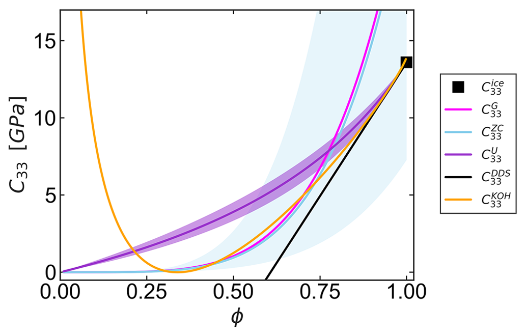
Figure 1 Evolution of the elastic modulus C₃₃ as a function of volume fraction ϕ for all discussed models: density-based parameterization proposed by Gerling et al. (2017) ($C_{\mathrm{33}}^{\mathrm{G}}$; see Eq. 4; expected range of validity $\mathrm{0.1}<\mathit{\varphi }<\mathrm{0.4}$), band of values predicted by Srivastava et al. (2016) ($C_{\mathrm{33}}^{\mathrm{ZC}}$; see Eq. 8; expected range of validity $\mathrm{0.109}<\mathit{\varphi }<\mathrm{0.59}$), band of values predicted by the Hashin–Shtrikman upper bound ($C_{\mathrm{33}}^{\mathrm{U}}$; see Eq. 9), elastic modulus for dilute dispersions ($C_{\mathrm{33}}^{\mathrm{DDS}}$; see Eq. 6; valid for high ice volume fractions), and the empirical relationship by Kohnen (1972) ($C_{\mathrm{33}}^{\mathrm{KOH}}$; see Eq. 5; expected range of validity $\mathrm{0.43}<\mathit{\varphi }<\mathrm{0.9}$8) are shown as a function of the volume fraction (ϕ) with continuous lines. The black square represents the maximum value of the elastic modulus in the C₃₃ direction for ice volume fraction ϕ=1. The shaded area for the anisotropic models represents the range of values between the two aspect ratios α=1.7 and α=0.6.

2.6 The remedy: matching asymptotics

The best of all existing models can be combined in a single model by constructing an empirical transition model that (i) increases as a power law for low volume fraction, (ii) includes anisotropy but with vanishing influence when approaching ice, and (iii) approaches the limiting behavior of dilute air bubbles for low porosity. Due to the properties of the HS bounds (correct limiting behavior of the bounds for low and high volume fraction, rational function for intermediate volume fractions), this can be achieved by using a transformation in the following form, in which the HS bound $C_{ij}^{\mathrm{U}}$ is normalized by $C_{ij}^{\mathrm{ice}}$ as

$$\begin{array}{}\text{(11)}& C_{ij}^{\mathrm{PW}}=C_{ij}^{\mathrm{ice}}{f}_{ij}\left({\displaystyle \frac{C_{ij}^{\mathrm{U}}}{C_{ij}^{\mathrm{ice}}}}\right),\end{array}$$

with an empirical transition function $f_{ij}:[\mathrm{0},\mathrm{1}]\to [\mathrm{0},\mathrm{1}]$ for each component of the elasticity tensor. Given that the HS bound approaches the limiting behavior of dilute dispersions for x→1 (Hashin and Shtrikman, 1962), the transition functions must obey f_ij(x)∼x for x→1. Further, since the modulus increases as a power law for lower volume fractions, the scaling function must behave as f_ij(x)∼x^β for x→0. These two asymptotics can be matched in the following empirical form:

$$\begin{array}{}\text{(12)}& f_{ij}\left(x\right)={\displaystyle \frac{x^{\mathit{\beta }}}{\mathit{\xi }(\mathrm{1}-x)+x^{\mathit{\beta }-\mathrm{1}}}}\sim \left\{\begin{array}{ll}{x}^{\mathit{\beta }}/\mathit{\xi },& \mathrm{for}x\to \mathrm{0}\\ x,& \mathrm{for}x\to \mathrm{1},\end{array}\right.\end{array}$$

which has the correct asymptotic behavior and contains only two free parameters. The first free parameter β ensures that at low volume fraction the modulus increases as a power law of the ice volume fraction. The second free parameter ξ acts, on the one hand, as a modification of the prefactor in the power law and, on the other hand, as the transition scale that controls the crossover to f(x)∼x. Equations (11) and (12) together with Eq. (9) constitute our empirical model that depends on density and anisotropy in a physically consistent way. The corresponding tensor components are henceforth referred to as $C_{ij}^{\mathrm{PW}}$, which will be analyzed and parameterized in the following from snow, firn, and ice tomography samples and finite-element simulations of the elastic modulus.

3 Material and computational methods

3.1 Tomography samples

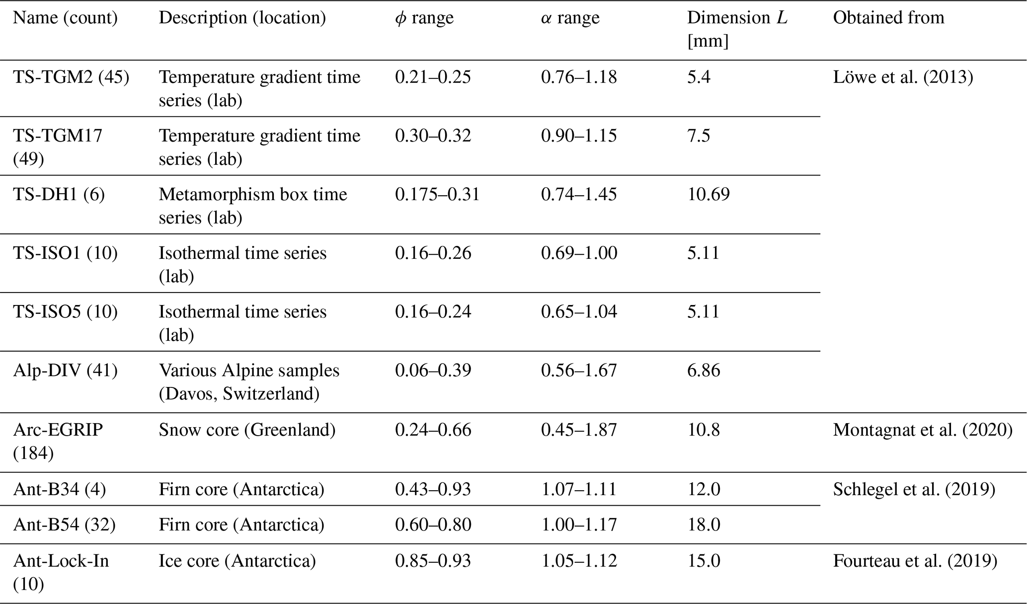
For the parameterization of snow elastic properties we used 391 microstructure images of snow, firn, and bubbly ice obtained with the help of μCT. Samples are taken from previous work and include laboratory, Alpine, Arctic, and Antarctic snow and ice. A brief description is given in Table 1. We considered the full range of porosities ranging from 0.06–0.93 and anisotropy ratios α ranging from 0.45–1.87. Note that all samples are cubic, with the same length L in the x, y, and z directions.

Löwe et al. (2013)Montagnat et al. (2020)Schlegel et al. (2019)Fourteau et al. (2019)

Table 1 μCT samples used for the parameterization of the elasticity tensor.

3.2 Correlation functions

We use tomography images of snow to compute the correlation functions of snow microstructures to calculate the anisotropy. As dry snow is a two-phase composite material consisting of air and ice phases, the indicator function ℐ(x) accounts for the spatial distribution of ice and air and is denoted by

$$\begin{array}{}\text{(13)}& \mathcal{I}\left(\mathcal{x}\right)=\left\{\begin{array}{ll}\mathrm{1}& \mathrm{if}\mathit{x}\in \mathrm{ice},\\ \mathrm{0}& \mathrm{if}\mathit{x}\in \mathrm{air}.\end{array}\right.\end{array}$$

The two-point correlation function χ(r) (Torquato, 2002b) entails information about the phase correlation of the end points of the vector r and is defined by

$$\begin{array}{}\text{(14)}& \mathit{\chi }\left(\mathit{r}\right)=\langle \mathcal{I}(\mathit{x}\mathbf{+}\mathit{r})\mathcal{I}\left(\mathit{x}\right)\rangle -{\mathit{\varphi }}^{\mathrm{2}}.\end{array}$$

We assume a statistically homogeneous material, where χ is independent of the reference point x∈ℝ³. The function χ(r) is computed from 3D images via a fast Fourier transformation (Krol and Loewe, 2016; Löwe et al., 2013). Correlation lengths ℓ_z,ℓ_x, and ℓ_y are obtained by fitting χ_q(r) along the Cartesian coordinate axes $q=x,y,$ and z to an exponential function ${\mathit{\chi }}_q\left(\mathit{r}\right)={\mathit{\chi }}_{q,\mathrm{0}}\exp (-r/{\mathrm{\ell }}_q)$. From this, the geometrical anisotropy parameter is defined by $\mathit{\alpha }={\mathrm{\ell }}_z/{\mathrm{\ell }}_{xy}$.

3.3 Geometrical fabric tensor

Srivastava et al. (2016) showed that the choice of the fabric tensor M computed by either mean intercept length (MIL), star length distribution (SLD), or star volume distribution (SVD) methods did not play a significant role in the computation of the effective elasticity tensor of snow. Therefore, we use the depolarization tensor M^* given in Torquato (2002a), which is based on two-point correlation lengths to estimate the structural anisotropy of the microstructure. Using M^* allows us to connect to previous work (Löwe et al., 2013; Montagnat et al., 2020; Calonne et al., 2015; Leinss et al., 2016) where this orientation tensor was employed to determine the anisotropic effective thermal conductivity and permittivity of snow. Analogous to MIL, M^* is the symmetric depolarization tensor of a three-dimensional ellipsoid with the eigenvalues in the principle axes frame given by elliptical integrals, whose trace is unity (Torquato, 2002a). In the case of transverse isotropy around the z axis, the depolarization tensor computed from two-point correlation function χ(r) reduces to

$$\begin{array}{}\text{(15)}& {\mathit{M}}^{*}=\left[\begin{array}{ccc}Q\left(\mathit{\alpha }\right)& \mathrm{0}& \mathrm{0}\\ \mathrm{0}& Q\left(\mathit{\alpha }\right)& \mathrm{0}\\ \mathrm{0}& \mathrm{0}& \mathrm{1}-\mathrm{2}Q\left(\mathit{\alpha }\right)\end{array}\right].\end{array}$$

The definition of the function Q(α) in terms of anisotropy ratio α is given in Appendix C.

3.4 FEM simulations

Finite-element method (FEM) simulations were performed using the code from Garboczi (1998) on all the CT images to determine the elasticity tensor of the snow microstructure by employing periodic boundary conditions. For these simulations, we assumed elastically isotropic ice with a shear modulus G^ice=3.52 GPa and a bulk modulus K^ice=8.9 GPa, corresponding to a temperature of −16 °C (Petrenko and Whitworth, 2002). We performed FEM simulations for five load states derived from Cartesian basis vectors in the six-dimensional deformation space. The deformation ε of the five load states is taken from the set $\mathit{\{}{\mathit{\epsilon }}_{\mathrm{0}}{e}_{\mathrm{11}},{\mathit{\epsilon }}_{\mathrm{0}}{e}_{\mathrm{22}},{\mathit{\epsilon }}_{\mathrm{0}}{e}_{\mathrm{33}},{\mathit{\epsilon }}_{\mathrm{0}}(e_{\mathrm{13}}+e_{\mathrm{23}}),{\mathit{\epsilon }}_{\mathrm{0}}{e}_{\mathrm{12}}\mathit{\}}$, with ε₀=0.01 and with e₁₁ to e₁₂ being unit vectors in the deformation space. Note that we combined load states 13 and 23 for the fourth deformation state.

Next, for each sample the five independent components of the elasticity tensor C (see Eq. 2) are estimated by minimizing the L2 norm of $\mathit{\sigma }-{\mathit{C}}^{\mathrm{FEM}}:\mathit{\epsilon }=\mathrm{0}$, where σ and ε are the stress and deformation states from the simulations. The specific choice of load states naturally implies different weights for the elasticity components during the least-squares optimization, as, for instance, $C_{\mathrm{33}}^{\mathrm{FEM}}$ is only involved in the e₃₃ load state. This optimization strategy ensures the resulting elasticity tensor is transverse isotropic and incompressible. It also ensures that the components are consistently estimated through the several load states in which they play a role.

To assess whether we fulfill the representative volume element (RVE) criterion, we employ the estimate of Wautier et al. (2015), which is based on correlation functions. RVE convergence is deemed to be satisfied when the ratio of linear sample size L (given in Table 1) and the correlation length l ($\sqrt[\mathrm{3}]{l_x{l}_y{l}_z}$) exceed 30. From this, we deduce that 92 % of our samples fulfill this requirement, while 8 % of the samples do not fulfill it but were still kept in the data set, as they do not appear as outliers in our results. The latter samples have ice volume fractions ranging from 0.11 to 0.66.

3.5 Reparameterization of existing models

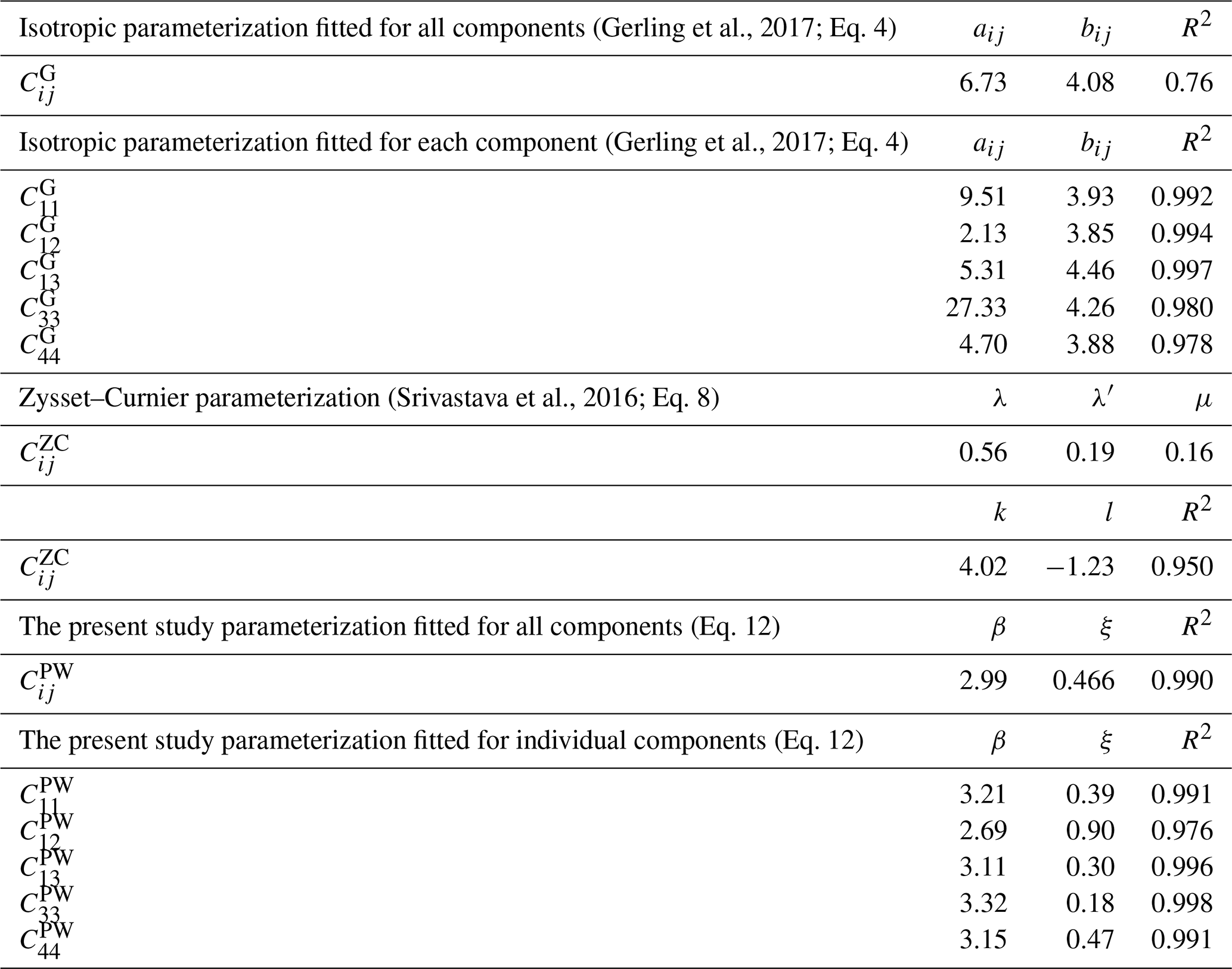
From the simulations we also reparameterize existing models from Sect. 2. The unknown parameters in the Gerling model (a_ij and b_ij), the Zysset–Curnier model ($\mathit{\lambda },\mathit{\lambda }{}^{\prime },\mathit{\mu },k$, and l), and the present model (ξ and β) are obtained by performing least-squares regression on the simulated elasticity tensor components against the models from Sect. 2.2. The free parameters of all models were adjusted using a log transformation of the elasticity tensor component, as done in Srivastava et al. (2016) or Zysset (2003).

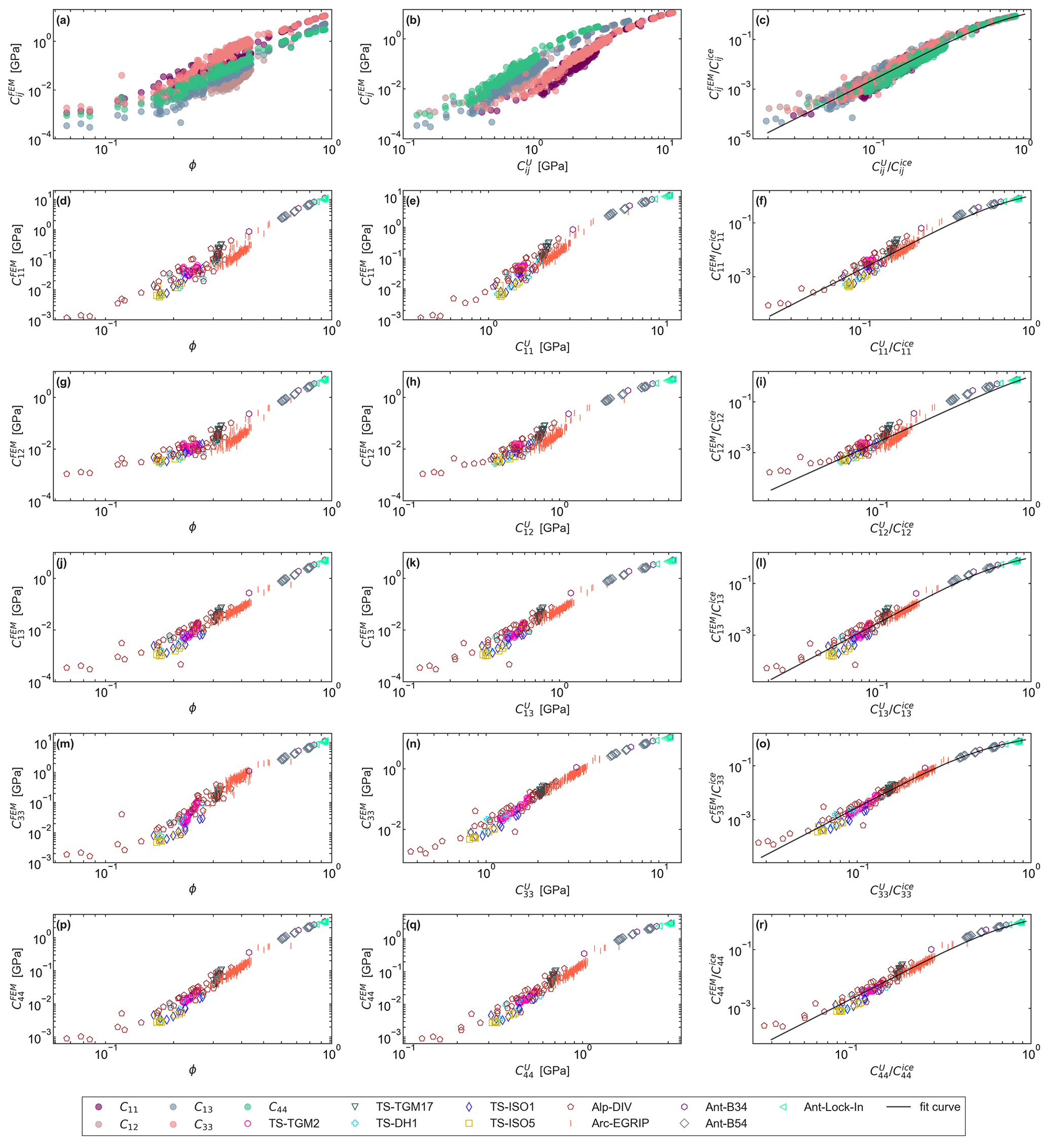
Figure 2 Simulated elasticity components $C_{ij}^{\text{FEM}}$ (different rows) are shown as a function of volume fraction ϕ (left column), as a function of the HS upper bound $C_{ij}^{\text{U}}$ (middle column), and in the normalized version $C_{ij}^{\text{U}}/C_{ij}^{\text{ice}}$ (right column). The black curve represents the parameterization derived for all the components (two parameters each). In the top row, the color scheme represents the components of the elasticity tensor. In the other rows, the colors and symbols represent the different samples considered in the present study, presented in Table 1.

4 Results

4.1 Present study parameterization

Figure 2 shows an overview of all results by plotting the simulated elasticity components $C_{ij}^{\text{FEM}}$ (different rows) against the ice volume fraction (column 1), the HS upper bound (column 2), and the normalized representation from Eq. (11). In the top row (Fig. 2a–c), all elasticity components from all the samples are represented with different colors depending on the component of the elasticity tensor. In contrast, in the rest of the rows, only one component is represented at a time, and the colors and symbols highlight the different samples, as defined in Table 1. The figure shows that the scatter of the simulated elasticity tensor components ($C_{ij}^{\text{FEM}}$) is maximal when plotted as a function of ice volume fraction ϕ (left column) and that this scatter is reduced when plotted as a function of HS upper bound $C_{ij}^{\text{U}}$ instead (middle column).

Next, we use the improved correlation between $C_{ij}^{\text{FEM}}$ and $C_{ij}^{\text{U}}$ to derive the parameterization for each component according to Eq. (11), shown as the black curves (right column). Note that the nonlinear transition behavior from the power law increases at low densities when approaching the value of ice is well captured for all the components. The performance, however, slightly differs for individual tensor components and is the best for C₃₃. We also stress that the data collapse for all tensor components in the normalized plot indicates that only two parameters are sufficient to obtain a decent picture of elasticity from Eq. (12).

Gerling et al., 2017Gerling et al., 2017Srivastava et al., 2016

Table 2 Parameters and regression coefficient obtained from the least-squares regression of the simulated elastic modulus employing different models on the entire data set.

4.2 Comparison to previous parameterizations

To examine the performance of the parameterization derived by fitting either individual components (see the top row of Fig. 3) or all the components of the elastic modulus simultaneously (see the bottom row of Fig. 3), we show a scatterplot of the C₃₃ component of the elastic modulus evaluated from numerical simulations vs. the three parameterizations: the density-based parameterization from Gerling (left), the Zysset–Curnier parameterization (middle), and the present study parameterization (right). As with Fig. 2, the colors and symbols in the top row of Fig. 3 represent the different samples, while the colors in the bottom row represent the components of the elasticity tensor. A detailed overview of the parameters obtained for different parameterizations and their coefficient of regression is given in Table 2. Note that these parameters differ from the values obtained in the original publication as the models were readjusted to fit our FEM simulations as explained in Sect. 3.5.

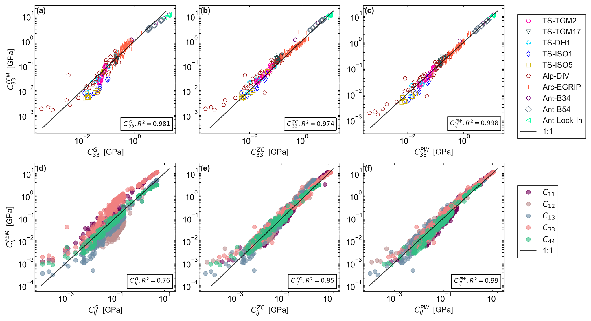
Figure 3 Comparison of simulated elastic modulus ($C_{\mathrm{33}}^{\mathrm{FEM}}$) to the Gerling et al. (2017) (G) density-based power-law model given by Eq. (4), the Zysset–Curnier (ZC) model (Srivastava et al., 2016) given by Eq. (8), and the present-work parameterization (PW) given by Eq. (12) (from left to right). The given R² values correspond to the performance of the parameterization by fitting (a, b, c) individual or (d, e, f) all components, respectively. In panels (a), (b), and (c) the colors and symbols represent the different samples considered in the present study, presented in Table 1. In panels (d), (e), and (f) the color scheme represents the components of the elasticity tensor.

4.3 Comparison at high ice volume fractions

The improvement of the prediction of the elastic modulus using the present-work parameterization $C_{\mathrm{33}}^{\mathrm{PW}}$ at high volume fraction is compared with elastic modulus determined by the formula from Kohnen (1972) in Eq. (5), where the P-wave velocity of ice $v_{\mathrm{p}}^{\mathrm{ice}}$ is calculated once by using the geometrical elastic modulus of ice ($v_{\mathrm{p}}^{\mathrm{ice}}=(C_{\mathrm{33}}^{\mathrm{ice}}/{\mathit{\rho }}^{ice}{)}^{\mathrm{0.5}}$) and with the literature P-wave velocity of ice $v_{\mathrm{p}}^{\mathrm{ice}}\approx \mathrm{3900}$ m s⁻¹, which was notably estimated through vertical seismic profiling in Antarctica (Diez, 2013). This comparison is depicted in Fig. 4. We see that $C_{\mathrm{33}}^{\mathrm{KOH}}$, based on the elastic modulus of ice used in this work, exactly approaches the correct limit and is in line with our parameterization $C_{\mathrm{33}}^{\mathrm{PW}}$ and the limit of elastic modulus for bubbly ice $C_{\mathrm{33}}^{\mathrm{DDS}}$. This validity of the $C_{\mathrm{33}}^{\mathrm{PW}}$, $C_{\mathrm{33}}^{\mathrm{KOH}}$, and $C_{\mathrm{33}}^{\mathrm{DDS}}$ parameterizations at high density is also confirmed by their agreement with the simulated $C_{\mathrm{33}}^{\mathrm{FEM}}$ values.

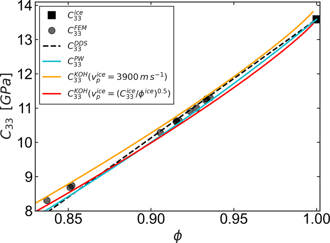
Figure 4 Comparison of present-work parameterization $C_{\mathrm{33}}^{\mathrm{PW}}$ with the elastic modulus $C_{\mathrm{33}}^{\mathrm{KOH}}$ determined by the empirical formula from Kohnen (1972), which is based on P-wave velocity and density (P-wave velocity is determined from structural elastic modulus of ice), the elasticity modulus $C_{\mathrm{33}}^{\mathrm{KOH}}$ obtained by taking P-wave velocity as 3900 ms⁻¹, and the upper bound of elastic modulus for dilute dispersion ($C_{\mathrm{33}}^{\mathrm{DDS}}$). The black square represents the elastic modulus of ice ($C_{\mathrm{33}}^{\mathrm{ice}}$). The black dots correspond to simulations in this density regime ($C_{\mathrm{33}}^{\mathrm{FEM}}$).

4.4 Relative influence of geometrical anisotropy and density

While the elasticity of snow, firn, and ice is predominantly controlled by density, we can now quantify the additional controls of geometrical anisotropy. To assess the distribution of geometrical anisotropy of the entire data set, we plot the structural anisotropy parameter $\mathit{\alpha }={\mathrm{\ell }}_z/{\mathrm{\ell }}_{xy}$ for all 391 microstructures as a function of the ice volume fraction in Fig. 5a. The highest anisotropy parameter (α=1.87, ϕ=0.39) is registered by an Arc-EGRIP sample.

The potential error induced by assuming isotropy (α=1) in determining parameterization of elastic modulus is shown in an error plot in Fig. 5b. Here, the error $C_{\mathrm{33}}^{\text{PW}}(\mathit{\varphi },\mathit{\alpha })-C_{\mathrm{33}}^{\text{PW}}(\mathit{\varphi },\mathrm{1})/C_{\mathrm{33}}^{\text{PW}}(\mathit{\varphi },\mathrm{1})$ is shown as a two-dimensional contour plot as a function of the ice volume fraction and the anisotropy parameter α. The relative error gives the percentage error induced between the elastic modulus computed as a function of anisotropy and as a function of isotropy, with zero relative error for isotropic structures. Figure 5 presents the slice view of the microstructure for three different cases of α (α>1, α=1, and α<1). Note the vertical (α>1) and horizontal (α<1) geometrical orientation of the ice matrix.

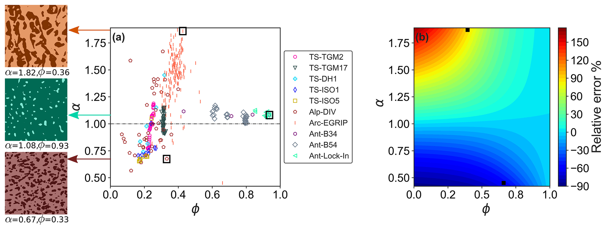
Figure 5 (a) Structural anisotropy of the microstructures (α) is plotted as a function of volume fraction ϕ. Isotropy is represented by the dashed line for α=1. The three square boxes represent the three different geometrical anisotropic ratios α>1 (prolate inclusions), α=1 (isotropic), and α<1 (oblate inclusions) present in our data, for which a slice view of the microstructure in the yz plane is presented. (b) Contour plot showing $C_{\mathrm{33}}^{\text{PW}}(\mathit{\varphi },\mathit{\alpha })-C_{\mathrm{33}}^{\text{PW}}(\mathit{\varphi },\mathrm{1})/C_{\mathrm{33}}^{\text{PW}}(\mathit{\varphi },\mathrm{1})$ as a function of anisotropy and volume fraction. The two black squares represents the relative error at the maximum and minimum anisotropy ratios α=1.87 and α=0.45 which occur in the present data set in (a). The color bar represents the percentage of relative error computed for different geometrical anisotropic microstructures considered. Table 1 provides the description of the samples.

Figure 5 shows that the structural anisotropy α is an important component of the parameterization proposed in this work. However, as it is not straightforward to measure the structural anisotropy and as elasticity is highly sensitive to density, one may wonder how the errors induced by neglecting anisotropy compare to typical errors due to uncertainties in the density measurement. To answer this question, we compared the impact of neglecting anisotropy (that is to say assuming α=1) to that of a typical 5 % uncertainty when measuring density using μCT (Proksch et al., 2015; Hagenmuller et al., 2016). Specifically, we applied our parameterization of the C₃₃ component to the following three cases: case 1, which corresponds to the ideal case of taking into account geometrical anisotropy (α≠1) and assuming no uncertainty in density; case 2, which corresponds to a case where geometrical anisotropy is accounted for (α≠1) but with a 5 % uncertainty in density; and case 3, which corresponds to the case where geometrical anisotropy is neglected (α=1) but without density uncertainty. These three cases are applied to the Arc-EGRIP samples ($\mathrm{0.45}<\mathit{\alpha }<\mathrm{1.87}$ and $\mathrm{0.24}<\mathit{\varphi }<\mathrm{0.66}$), which underwent temperature gradient metamorphism experiments under natural conditions, and to the TS-TGM17 samples ($\mathrm{0.9}<\mathit{\alpha }<\mathrm{1.15}$ and $\mathrm{0.30}<\mathit{\varphi }<\mathrm{0.32}$), which in contrast underwent TGM in controlled conditions. They are visible in Fig. 6 alongside the estimation of the C₃₃ component directly derived from the FEM simulations, which serves as a reference. Neglecting anisotropy (case 3) leads to average errors of 39.8 % and 21.7 % for the Arc-EGRIP and TS-TGM17 samples, respectively. A 5 % error in density, while taking into account anisotropy (case 2), yields average errors of 23 % and 11.96 % for the Arc-EGRIP and TS-TGM17 samples, respectively. This is to be compared with average errors of 14.56 % and 11.96 % when anisotropy is considered (case 1) and when there is no error in density.

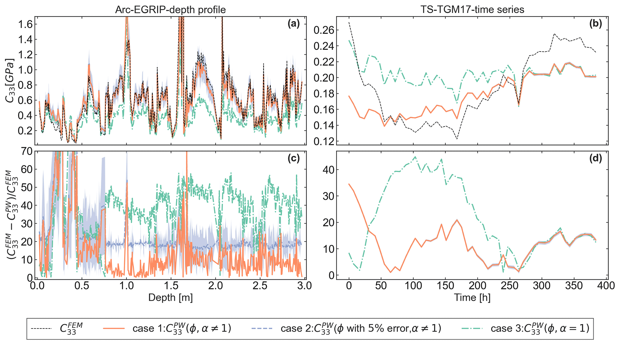
Figure 6 Comparison of the elastic modulus calculated from FEM simulations $C_{\mathrm{33}}^{\mathrm{FEM}}$ to present-work parameterization $C_{\mathrm{33}}^{\mathrm{PW}}$ for (a) Arc-EGRIP samples as a function of depth and (b) one of the TGM time series (TS-TGM17). $C_{\mathrm{33}}^{\mathrm{PW}}$ is computed for the following three cases: case 1, accounting for anisotropy without uncertainty in density $C_{\mathrm{33}}^{\mathrm{PW}}(\mathit{\varphi },\mathit{\alpha }\ne \mathrm{1})$; case 2, accounting for anisotropy with 5 % uncertainty in ϕ $C_{\mathrm{33}}^{\mathrm{PW}}(\mathit{\varphi }$ with 5 % error, α≠1); and case 3, not accounting for anisotropy without uncertainty in density $C_{\mathrm{33}}^{\mathrm{PW}}(\mathit{\varphi },\mathit{\alpha }=\mathrm{1})$. Panels (c) and (d) show the norm of the relative errors of the three cases compared to the finite-element results. The shaded area for case 2 represents the spread resulting from a 5 % uncertainty in density.

4.5 Comparison of geometrical and crystallographic anisotropy

To assess the geometrical anisotropy in reference to the crystallographic anisotropy when determining the elastic properties of snow, firn, and ice for a given ice volume fraction, we plot the geometrical Thomsen parameter ϵ_geom, obtained from Eq. (3), against ϕ in Fig. 7. For comparison, we also show the maximum crystallographic anisotropy that can be theoretically obtained, which is the known value of monocrystalline ice at zero porosity (ϕ=1) given by ${\mathit{ϵ}}_{\text{cryst}}=-\mathrm{0.0356}$ (Petrenko and Whitworth, 2002). The expected (but unknown) decay of ϵ_cryst for ϕ<1 is shown as a schematic (see Discussion).

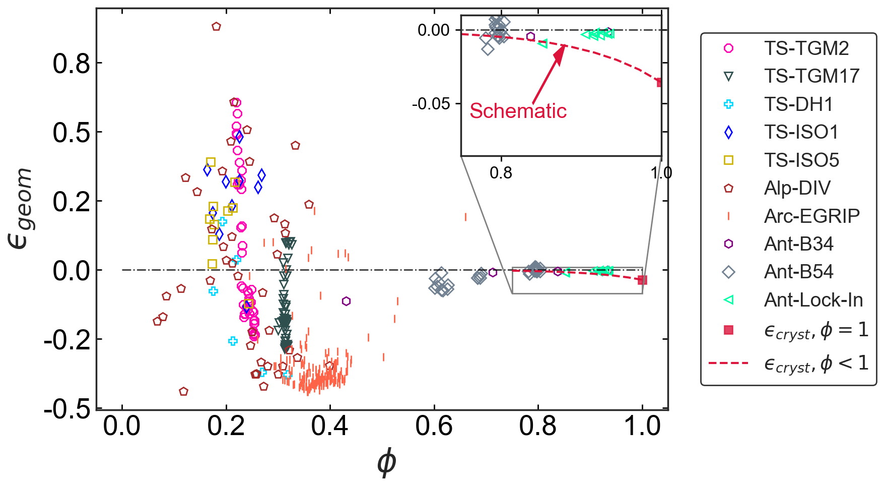
Figure 7 Geometrical and crystallographic Thomsen parameters, ϵ_geom and ϵ_cryst, plotted as a function of volume fraction ϕ to show the predominant influence of anisotropy (geometrical and crystallographical) on elastic properties. The dashed red line illustrates a schematic representation of the expected behavior of crystallographic anisotropy ϵ_cryst for ϕ<1. Sample name descriptions are given in Table 1.

5 Discussion

5.1 Summary of main results

The proposed empirical parameterization offers a crucial advantage by being applicable across the range of natural ice volume fractions, enabling accurate predictions of the effective elastic modulus (see Fig. 3). This broad range of applicability is supported by the fact that some of the temperature gradient experiment samples used in this study have been independently compared with natural Arctic snow in terms of geometrical anisotropy (Leinss et al., 2020). Furthermore, these anisotropic samples fall into the intermediate density range (250 to 500 kg m³), where geometrical anisotropy exerts a substantial influence, in contrast with the lesser dominance of structural anisotropy at low and high densities. Therefore, we expect that our parameterization is sufficiently generic to capture typical anisotropic structures in snow. Furthermore, the samples used to derive the parameterization are diverse regarding their conditions of formation. Consequently, we expect this parameterization to yield reasonably accurate predictions of elastic properties for the whole range of natural porous snow, firn, and ice formations.

Previous parameterizations of the elastic modulus, based either on density alone (Eq. 4; Gerling et al., 2017) or on density and anisotropy (Eq. 8; Srivastava et al., 2016), can significantly overestimate the elastic modulus when applied outside their validity range (see Fig. 1). The advantage of HS bounds (Eq. 9) is that they comply with the limiting behavior of bubbly ice (see Sect. 2.6) and do not overestimate the elastic properties as they approach high volume fractions and incorporate the anisotropy (see Fig. 1). For constructing the empirical parameterization, we exploited the fact that the elastic modulus should asymptotically tend to the behavior of randomly diluted spheres, reflecting the fact that low-porosity ice from ice cores mainly consists of convex (sphere-like) air cavities (Fourteau et al., 2019). The validity of this assumption is reflected by Fig. 4, which shows that numerical simulations coincide very well with the theoretical prediction of elasticity for dilute dispersions of spherical cavities (see Eq. 6).

The relatively moderate change in the regression coefficient of our $C_{\mathrm{33}}^{\mathrm{PW}}$ in comparison to previous parameterizations $C_{\mathrm{33}}^{\mathrm{G}}$ and $C_{\mathrm{33}}^{\mathrm{PW}}$ (see Fig. 3) reflects the fact that anisotropy only has a subdominant influence on elasticity, while density remains the main parameter. However, capturing these subdominant influences may be very important for advanced microstructure characterization by alternative means, such as capturing macroscopic physical properties remotely (Leinss et al., 2016). Moreover, as shown in Sect. 4.4, neglecting anisotropy is the main source of error when estimating the elastic properties of a sample whose density has been measured with state-of-the-art techniques (Proksch et al., 2015; Hagenmuller et al., 2016).

Our parameterization of the elastic modulus is a good alternative to computationally expensive FEMs. Although other theoretical approximations, such as the self-consistent (SC) approximation, were previously employed by Wautier et al. (2015) to predict the effective elastic properties and by Calonne et al. (2019) to predict the effective thermal conductivity for the entire range of densities, SC approximations are based on implicit equations that need to be solved (Torquato, 2002a). Torquato (1998) showed that SC approximations give inadequate approximation of effective moduli of dispersions and overestimate the effective moduli in comparison to rigorous bounds. In contrast, the limiting behavior of the Hashin–Shtrikman bounds can provide an explicit formula for effective moduli.

It is notable that the range of the elastic modulus varies for each tensor component (see Fig. 2b) plotted as a function of the Hashin–Shtrikman bound. Hence, we parameterize the elastic modulus for each component shown in Fig. 2 (column 3), as described in Sect. 2.6 using Eq. (12), and the two parameters ξ and β for each component are given in Table 2. We also observed that all five components collapse onto a single curve when normalizing the simulated values by ice moduli ($C{}_{ij}^{\mathrm{FEM}}/C{}_{ij}^{\mathrm{ice}}$) and plotting them as a function of the normalized HS upper bound $(C{}_{ij}^{\mathrm{U}}/C{}_{ij}^{\mathrm{ice}})$. This helped with the prediction of all five components of the elastic modulus with only two parameters in contrast to five parameters given by the Zysset–Curnier parameterization used in Srivastava et al. (2016) for an orthotropic elasticity tensor.

5.2 Choice of the geometrical fabric tensor

Srivastava et al. (2016) demonstrated that the choice of the fabric tensor does not affect the prediction of anisotropy. Hence, the MIL fabric tensor, employed by the Zysset–Curnier parameterization in Srivastava et al. (2016), was replaced here by the symmetric depolarization tensor (orientation tensor) M^*. In this way, the current elasticity parameterization involves exactly the same microstructure parameter (ϕ,α) as previous permittivity or thermal conductivity parameterizations (Leinss et al., 2016; Löwe et al., 2013). Weng (1992) evaluated bounds using a similar depolarization tensor based on two-point correlation functions assuming ellipsoidal symmetry. Their results were consistent with those of the Hashin–Shtrikman bounds evaluated by Eshelby's tensor.

We note that the choice of the fabric tensor has an impact on the sign of the fit parameter (l) in the Zysset–Curnier parameterization, yielding a negative value here in contrast to Srivastava et al. (2016). This can be explained because our depolarization tensor M^* given by Eq. (15) yields a zero eigenvalue in the vertical direction for a vertically oriented microstructure. In contrast, the MIL fabric tensor is represented by 〈m_i⊗m_j〉, with a local director m_i, and is divided by its trace. If the orientation is in the m_i direction, then the corresponding eigenvalue in this direction is maximized. Therefore, the sign of the l parameter is reversed. A limitation of the MIL fabric tensor is, however, that it is not able to detect interfacial anisotropy; Odgaard (1997) evaluated a two-dimensional “Swiss cheese” microstructure where the MIL analysis predicted an isotropic geometry despite the obvious, anisotropic arrangement of the spheres. The result of the analysis was influenced by the isotropic interfaces between the phases. Similar results were also observed by Klatt et al. (2017): when the MIL analysis was performed on a Boolean model with aligned Reuleaux triangles, it resulted in circles. MIL determination based on standard line- or intersection-counting techniques used to determine MIL is time-consuming and sensitive to noise (Moreno et al., 2012).

5.3 Performance of the parameterization

Overall, the parameterization used in the present-work $C_{\mathrm{33}}^{\text{PW}}$, given by Eqs. (11)–(12), had excellent agreement (R²=0.99) when fit to all components simultaneously with two parameters in comparison to previous parameterizations from Srivastava et al. (2016) (volume-fraction- and fabric-dependent) and Gerling et al. (2017) (volume-fraction-dependent), which yielded the coefficients of determination R²=0.76 and R²=0.952, respectively (see Table 2 and Fig. 3). Figure 3d shows that the Gerling et al. (2017) density-based parameterization yields the best prediction for the component C₄₄ when derived by fitting all components. This is because the C₄₄ component values lie in between the diagonal component values C₁₁ and C₃₃ (typically higher values) and off-diagonal component values C₁₂ and C₁₃ (typically lower values). The highest improvement over density-based parameterizations is achieved for the C₃₃ component for the TS-TGM2, TS-TGM17, and Arc-EGRIP samples, which becomes apparent when plotted as a function of the HS upper bound or volume fraction (see Fig. 2). All of these samples have an ice matrix predominantly oriented in the z direction (see Fig. 5a) with the anisotropy ratio α>1. Such vertically oriented structures are generated by strong temperature gradient metamorphism (Calonne et al., 2012; Löwe et al., 2013; Leinss et al., 2020) occurring in the snow, firn, and ice. This is evident for temperature gradient time series (TS-TGM2 and TS-TGM17) from Fig. 5a, where we see the change from a horizontal orientation of ice matrix into a vertical orientation. The improvement of the prediction of the elastic modulus mainly in the z direction is consistent with previously derived properties such as thermal conductivity for snow (see Löwe et al., 2013). EastGRIP (Arc-EGRIP) samples extracted from the firn in Greenland also display a similar kind of geometrical anisotropy in the vertical direction (Montagnat et al., 2020).

To further test the performance of our parameterization, we considered ice volume fraction and correlation function data provided by Wautier et al. (2015). The data display values of α ranging from 0.65 to 1.26 and of ϕ ranging from 0.10 to 0.59. We applied our parameterization on these data using Eq. (12) and compared the obtained results to the elastic stiffness tensor computed from FEM simulations of Wautier et al. (2015) and Srivastava et al. (2016) and from the present work. We also added the other parameterizations derived from FEM simulations (namely Köchle and Schneebeli, 2014; Gerling et al., 2017), with ϕ ranging from 0.10 to 0.59. We found that PW parameterization applied to the data of Wautier et al. (2015) differs from the simulation results from Wautier et al. (2015). However, despite the scatter, both our FEM simulations and PW parameterization lie within the range of finite-element results from Srivastava et al. (2016), Köchle and Schneebeli (2014), and Gerling et al. (2017).

Using the new parameterization, it is possible to assess the maximum error in the prediction of elasticity if anisotropy is not taken into account (see Fig. 5b). As the relative error is not the same for microstructures with vertical and horizontal orientations of the ice matrix (see Fig. 5a), the error plot is nonsymmetric in α (see Fig. 5b). The relative error of the elastic modulus for vertical ice matrix orientation (TS-TGM2, TS-TGM17, and Arc-EGRIP) (α>1) (see the top half of Fig. 5b) is larger than 100 %. The relative error for horizontal orientation of ice matrix (α<1) seen for ϕ between snow to ice is up to −90 %. From Fig. 5a and b, it is clear that for intermediate volume fractions in the range $\mathrm{0.3}<\mathit{\varphi }<\mathrm{0.5}$, very different anisotropy values are possible for a similar density. Using the extreme values from Fig. 5b, the prediction of elastic modulus solely as a function of ϕ could miss variations of up to 200 %. For ϕ→1, the relative error must approach zero, since for vanishing porosity (polycrystalline) ice becomes geometrically isotropic.

5.4 Comparison of geometrical and crystallographical anisotropy

In Figs. 5a and 7 we see the typical evolution of the geometrical anisotropy in snow, firn, and ice, with a sharp increase in geometrical anisotropy with density in low-density snow and its survival up to high densities. Initially, at low density, snow exhibits a horizontal orientation of the ice matrix (Leinss et al., 2016). As the volume fraction increases from snow to firn, we observe the transition of the orientation to the vertical direction. This change is a result of temperature gradient metamorphism, which can be easily confirmed from the temperature gradient metamorphism experiments (TS-TGM2 and TS-TGM17) and also from the Arc-EGRIP data set (Leinss et al., 2020). The existence of geometrical anisotropy in polar snow is well known (Fujita et al., 2014; Moser et al., 2020) and can be quantitatively related to temperature gradient metamorphism (Montagnat et al., 2020). When the volume fraction of ice increases further from firn to bubbly ice, the microstructures relax to a geometrically isotropic state. This is a consequence of the gravitational settling and densification of snow (Leinss et al., 2020). However, we infer from Fig. 5a that the vertical geometrical anisotropy generated near the surface survives beyond the bubble close-off transition around ϕ≈0.92 that underlies the Ant-Lock-In data, as discussed in Fourteau et al. (2019). This raises the question of at which point exactly the crystallographic anisotropy becomes the dominant type of anisotropy.

To this end, we have quantified the geometrically elastic anisotropy by deriving the corresponding Thomsen parameter ϵ_geom for the entire range of ice volume fraction (see Fig. 7). This clearly reveals that the geometrical anisotropy dominates snow and firn for ice volume fraction ϕ<0.7 in our data. For bubbly ice, the situation is a bit more complicated. The crystallographic Thomsen parameter of ice ϵ_cryst shown in Fig. 7 is only valid for ϕ=1, where the geometrical Thomsen parameter ϵ_geom must vanish. However, it can be expected that in the range $\mathrm{0.7}<\mathit{\varphi }<\mathrm{1}$ the geometrical and crystallographic anisotropies are of similar magnitude since the crystallographic Thomsen parameter ϵ_cryst must decay from its ice value when increasing the porosity. To understand this phenomenon, one can assume a volume-filling monocrystal, with a Thomsen parameter ϵ_cryst that corresponds to the maximum possible crystallographic anisotropy. Now, if this volume is gradually filled with an isotropic inclusion of air, the anisotropic behavior of the hollowed monocrystal decays. This behavior is shown as a schematic line on the inset of Fig. 7 and highlights the importance of consideration of both kinds of anisotropies for very high density. Such an influence of very low porosity on the crystallographic fabric is also implied by the results of Hellmann et al. (2021).

For microstructures in the volume fraction range $\mathrm{0.7}<\mathit{\varphi }<\mathrm{1}$, it may thus be important in the future to consider the concurrent effects of crystallographical and geometrical anisotropy, as consideration is presently nonexistent. It is important to know the dominant anisotropy (geometrical or crystallographic) for a given volume fraction for the prediction of elastic properties. Previous studies mostly consider crystallographic anisotropy, which may, however, become dominant only very close to ϕ=1.

5.5 Applicability of the current parameterization

To ease the applicability of the present parameterization, we provide the Python scripts with the data and the necessary functions to compute the parameterized elasticity tensor as a function of a sample’s density and anisotropy and of the shear and bulk modulus of ice. Also, while the parameterization of the elasticity tensor was derived using the elastic properties of ice at −16 °C, one can directly transpose the parameterization to a different temperature. This is readily done by taking into account the temperature dependence of the ice elastic properties that appear in the parameterization. Finally, as the purely elastic behavior of a porous material does not depend on grain size explicitly but only on its microstructural shape (as seen in Eshelby's tensor described in Appendix B), the proposed parameterization is applicable regardless of the grain size of the considered sample.

6 Conclusions

Using a transformation of the anisotropic Hashin–Shtrikman bounds, we derived a new closed-form parameterization for the effective elasticity tensor as a function of the volume fraction and geometrical anisotropy applicable from fresh snow to bubbly ice. Thereby, we extend the set of parameterizations of physical parameters with a similar focus on the full range of volume fractions (Calonne et al., 2019; Picard et al., 2022). We have demonstrated the advantages over previous elasticity parameterizations in view of performance and the correct asymptotic behavior for bubbly ice. Given the distribution of naturally occurring geometrical anisotropy, the uncertainty range of elastic moduli predictions is up to 200 % for intermediate volume fractions of $\mathrm{0.3}<\mathit{\varphi }<\mathrm{0.5}$ if only density is considered in the parameterization.

The new parameterization is a crucial tool with different applications in cryospheric sciences. In particular, we seek to trigger new microstructure retrievals through advanced anisotropic inversion methods of seismic data (Wu et al., 2022). Along these lines, our results shed new light on the relative importance of the two different types of elastic anisotropy (crystallographic and geometrical) in snow and firn that may influence the interpretation of seismic measurements (Schlegel et al., 2019). The geometrical anisotropy clearly dominates the crystallographic anisotropy for ϕ<0.7 and must be taken into account when discussing anisotropy in near-surface seismics (Chaput et al., 2022). While the geometrical anisotropy quickly decays with depth, remainders still persist down to the close-off depth, and how concurrent fabrics (geometrical and crystallographic) will elastically interact in bubbly ice is yet to be investigated.

Appendix A: Isotropic elasticity tensor

The elasticity tensor in terms of bulk modulus K and shear modulus G for an isotropic case is given as

$$\begin{array}{}\text{(A1)}& \mathit{C}=\left[\begin{array}{cccccc}K+\mathrm{4}G/\mathrm{3}& K-\mathrm{2}G/\mathrm{3}& K-\mathrm{2}G/\mathrm{3}& \mathrm{0}& \mathrm{0}& \mathrm{0}\\ K-\mathrm{2}G/\mathrm{3}& K+\mathrm{4}G/\mathrm{3}& K-\mathrm{2}G/\mathrm{3}& \mathrm{0}& \mathrm{0}& \mathrm{0}\\ K-\mathrm{2}G/\mathrm{3}& K-\mathrm{2}G/\mathrm{3}& K+\mathrm{4}G/\mathrm{3}& \mathrm{0}& \mathrm{0}& \mathrm{0}\\ \mathrm{0}& \mathrm{0}& \mathrm{0}& G& \mathrm{0}& \mathrm{0}\\ \mathrm{0}& \mathrm{0}& \mathrm{0}& \mathrm{0}& G& \mathrm{0}\\ \mathrm{0}& \mathrm{0}& \mathrm{0}& \mathrm{0}& \mathrm{0}& G\end{array}\right],\end{array}$$

with Young's modulus as $E=\frac{\mathrm{9}KG}{\mathrm{3}K+G}$ and Poisson's ratio as $\mathit{\nu }=\frac{\mathrm{3}K-\mathrm{2}G}{\mathrm{2}(\mathrm{3}K+G)}$.

Appendix B: Eshelby's tensor

Eshelby's tensor S is defined in terms of elliptical integrals. For the case of a spheroidal inclusion with the semiaxis given in terms of correlations lengths ${\mathrm{\ell }}_x={\mathrm{\ell }}_y=a$ and ℓ_z=b, and with the symmetry axis aligned in the z direction embedded in a transverse isotropic comparison phase, this results in a transverse isotropic Eshelby's tensor, with the components of S_ijkl given in Torquato (2002a) and Parnell and Calvo-Jurado (2015) as follows:

$$\begin{array}{}\text{(B1)}& \begin{array}{rl}& S_{\mathrm{1111}}=S_{\mathrm{2222}}={\displaystyle \frac{\mathrm{3}}{\mathrm{8}(\mathrm{1}-v_{\mathrm{1}})}}{\displaystyle \frac{{\mathit{\alpha }}^{\mathrm{2}}}{{\mathit{\alpha }}^{\mathrm{2}}-\mathrm{1}}}+{\displaystyle \frac{\mathrm{1}}{\mathrm{4}(\mathrm{1}-v_{\mathrm{1}})}}\\ & [\mathrm{1}-\mathrm{2}{v}_{\mathrm{1}}-{\displaystyle \frac{\mathrm{9}}{\mathrm{4}({\mathit{\alpha }}^{\mathrm{2}}-\mathrm{1})}}]q,\\ & S_{\mathrm{3333}}={\displaystyle \frac{\mathrm{1}}{\mathrm{2}(\mathrm{1}-v_{\mathrm{1}})}}\mathit{\{}\mathrm{1}-\mathrm{2}{v}_{\mathrm{1}}+{\displaystyle \frac{\mathrm{3}{\mathit{\alpha }}^{\mathrm{2}}-\mathrm{1}}{{\mathit{\alpha }}^{\mathrm{2}}-\mathrm{1}}}\\ & -[\mathrm{1}-\mathrm{2}{v}_{\mathrm{1}}+{\displaystyle \frac{\mathrm{3}{\mathit{\alpha }}^{\mathrm{2}}}{{\mathit{\alpha }}^{\mathrm{2}}-\mathrm{1}}}]q\mathit{\}},\\ & S_{\mathrm{1122}}=S_{\mathrm{2211}}={\displaystyle \frac{\mathrm{1}}{\mathrm{4}(\mathrm{1}-v_{\mathrm{1}})}}\mathit{\{}{\displaystyle \frac{{\mathit{\alpha }}^{\mathrm{2}}}{\mathrm{2}(\mathit{\alpha }-\mathrm{1})}}\\ & -[\mathrm{1}-\mathrm{2}{v}_{\mathrm{1}}+{\displaystyle \frac{\mathrm{3}}{\mathrm{4}({\mathit{\alpha }}^{\mathrm{2}}-\mathrm{1})}}]q\mathit{\}},\\ & S_{\mathrm{1133}}=S_{\mathrm{2233}}={\displaystyle \frac{\mathrm{1}}{\mathrm{2}(\mathrm{1}-v_{\mathrm{1}})}}\mathit{\{}{\displaystyle \frac{-{\mathit{\alpha }}^{\mathrm{2}}}{{\mathit{\alpha }}^{\mathrm{2}}-\mathrm{1}}}\\ & +{\displaystyle \frac{\mathrm{1}}{\mathrm{2}}}[{\displaystyle \frac{\mathrm{3}{\mathit{\alpha }}^{\mathrm{2}}}{{\mathit{\alpha }}^{\mathrm{2}}-\mathrm{1}}}-(\mathrm{1}-\mathrm{2}{v}_{\mathrm{1}}\left)\right]q\mathit{\}},\\ & S_{\mathrm{3311}}=S_{\mathrm{3322}}={\displaystyle \frac{\mathrm{1}}{\mathrm{2}(\mathrm{1}-v_{\mathrm{1}})}}\mathit{\{}\mathrm{2}{v}_{\mathrm{1}}-\mathrm{1}-{\displaystyle \frac{\mathrm{1}}{{\mathit{\alpha }}^{\mathrm{2}}-\mathrm{1}}}\\ & +[\mathrm{1}-\mathrm{2}{v}_{\mathrm{1}}+{\displaystyle \frac{\mathrm{3}}{\mathrm{2}({\mathit{\alpha }}^{\mathrm{2}}-\mathrm{1})}}]q\mathit{\}},\\ & S_{\mathrm{1212}}={\displaystyle \frac{\mathrm{1}}{\mathrm{4}(\mathrm{1}-v_{\mathrm{1}})}}\mathit{\{}{\displaystyle \frac{{\mathit{\alpha }}^{\mathrm{2}}}{\mathrm{2}{\mathit{\alpha }}^{\mathrm{2}}-\mathrm{1}}}+[\mathrm{1}-\mathrm{2}{v}_{\mathrm{1}}\\ & -{\displaystyle \frac{\mathrm{3}}{\mathrm{4}({\mathit{\alpha }}^{\mathrm{2}}-\mathrm{1})}}\left]q\mathit{\right\}},\\ & S_{\mathrm{1313}}=S_{\mathrm{2323}}={\displaystyle \frac{\mathrm{1}}{\mathrm{4}(\mathrm{1}-v_{\mathrm{1}})}}\mathit{\{}\mathrm{1}-\mathrm{2}{v}_{\mathrm{1}}-{\displaystyle \frac{{\mathit{\alpha }}^{\mathrm{2}}+\mathrm{1}}{{\mathit{\alpha }}^{\mathrm{2}}-\mathrm{1}}}\\ & -{\displaystyle \frac{\mathrm{1}}{\mathrm{2}}}[\mathrm{1}-\mathrm{2}{v}_{\mathrm{1}}-{\displaystyle \frac{\mathrm{3}({\mathit{\alpha }}^{\mathrm{2}}+\mathrm{1})}{{\mathit{\alpha }}^{\mathrm{2}}-\mathrm{1}}}]q\mathit{\}},\end{array}\end{array}$$

where v₁ is the Poisson ratio of the comparison material, α is the aspect ratio of the spheroid given in terms of correlation lengths (${\mathrm{\ell }}_z/{\mathrm{\ell }}_{xy}$), and q is defined by

$$\begin{array}{}\text{(B2)}& q=\left\{\begin{array}{l}\frac{\mathit{\alpha }}{({\mathit{\alpha }}^{\mathrm{2}}-\mathrm{1}{)}^{\mathrm{3}/\mathrm{2}}}\left[\mathit{\alpha }\right({\mathit{\alpha }}^{\mathrm{2}}-\mathrm{1}{)}^{\mathrm{1}/\mathrm{2}}-{\cosh }^{-\mathrm{1}}\mathit{\alpha }],\mathit{\alpha }\ge \mathrm{1},\\ \frac{\mathit{\alpha }}{(\mathrm{1}-{\mathit{\alpha }}^{\mathrm{2}}{)}^{\mathrm{3}/\mathrm{2}}}[{\cos }^{-\mathrm{1}}\mathit{\alpha }-\mathit{\alpha }(\mathrm{1}-{\mathit{\alpha }}^{\mathrm{2}}{)}^{\mathrm{1}/\mathrm{2}}],\mathit{\alpha }\le \mathrm{1}.\end{array}\right.\end{array}$$

Several limits of Eshelby's tensor for transverse isotropic materials can be derived. For ice matrix orientation with needle-shaped structures $(\mathit{\alpha }\to \mathrm{\infty },q=\mathrm{1})$, Eshelby's tensor reads

$$\begin{array}{}\text{(B3)}& \begin{array}{rl}& S_{\mathrm{1111}}=S_{\mathrm{2222}}={\displaystyle \frac{\mathrm{5}-\mathrm{4}{v}_{\mathrm{1}}}{\mathrm{8}(\mathrm{1}-v_{\mathrm{1}})}},S_{\mathrm{3333}}=\mathrm{0},\\ & S_{\mathrm{1122}}=S_{\mathrm{2211}}={\displaystyle \frac{\mathrm{4}{v}_{\mathrm{1}}-\mathrm{1}}{\mathrm{8}(\mathrm{1}-v_{\mathrm{1}})}},\\ & S_{\mathrm{1133}}=S_{\mathrm{2233}}={\displaystyle \frac{v_{\mathrm{1}}}{\mathrm{2}(\mathrm{1}-v_{\mathrm{1}})}},\\ & S_{\mathrm{3311}}=S_{\mathrm{3322}}=\mathrm{0},S_{\mathrm{1212}}={\displaystyle \frac{\mathrm{3}-\mathrm{4}{v}_{\mathrm{1}}}{\mathrm{8}(\mathrm{1}-v_{\mathrm{1}})}},\\ & S_{\mathrm{1313}}=S_{\mathrm{2323}}={\displaystyle \frac{\mathrm{1}}{\mathrm{4}}}.\end{array}\end{array}$$

For inclusion with disk-shaped structures $(\mathit{\alpha }=\mathrm{0},q=\mathrm{0})$, the components of Eshelby's tensor are then given by

$$\begin{array}{}\text{(B4)}& \begin{array}{rl}{S}_{\mathrm{3333}}& =\mathrm{1},S_{\mathrm{3311}}=S_{\mathrm{3322}}={\displaystyle \frac{v_{\mathrm{1}}}{\mathrm{1}-v_{\mathrm{1}}}},\\ & S_{\mathrm{1313}}=S_{\mathrm{2323}}={\displaystyle \frac{\mathrm{1}}{\mathrm{2}}}.\end{array}\end{array}$$

Appendix C: Definition of function Q(α)

For the evaluation of the depolarization tensor M^* in Eq. (15) the definition of function Q(α) is given as (Torquato, 2002a)

$$\begin{array}{}\text{(C1)}& Q=\left\{\begin{array}{l}\frac{\mathrm{1}}{\mathrm{2}}\mathit{\{}\mathrm{1}+\frac{\mathrm{1}}{{\mathit{\alpha }}^{\mathrm{2}}-\mathrm{1}}[\mathrm{1}-\frac{\mathrm{1}}{\mathrm{2}{\mathit{\chi }}_b\left(\mathit{\alpha }\right)}\ln \left(\frac{\mathrm{1}+{\mathit{\chi }}_b\left(\mathit{\alpha }\right)}{\mathrm{1}-{\mathit{\chi }}_b\left(\mathit{\alpha }\right)}\right)\left]\mathit{\right\}},\mathit{\alpha }>\mathrm{1},\\ \frac{\mathrm{1}}{\mathrm{2}}\mathit{\{}\mathrm{1}+\frac{\mathrm{1}}{{\mathit{\alpha }}^{\mathrm{2}}-\mathrm{1}}[\mathrm{1}-\frac{\mathrm{1}}{{\mathit{\chi }}_b\left(\mathit{\alpha }\right)}\mathrm{atan}\left({\mathit{\chi }}_a\right(\mathit{\alpha }\left)\right)\left]\mathit{\right\}},\mathit{\alpha }<\mathrm{1},\end{array}\right.\end{array}$$

with ${\mathit{\chi }}_a(\mathit{\alpha }{)}^{\mathrm{2}}=-{\mathit{\chi }}_b(\mathit{\alpha }{)}^{\mathrm{2}}=\mathrm{1}/{\mathit{\alpha }}^{\mathrm{2}}-\mathrm{1}$. For this case, α=1 and $Q=\mathrm{1}/\mathrm{3}$.