the Creative Commons Attribution 4.0 License.
the Creative Commons Attribution 4.0 License.
 | 04 Jan 2024
Retrieval of snow water equivalent from dual-frequency radar measurements: using time series to overcome the need for accurate a priori information
Joel T. Johnson
Jack Dechow
Leung Tsang
Firoz Borah
Edward J. Kim
Measurements of radar backscatter are sensitive to snow water equivalent (SWE) across a wide range of frequencies, motivating proposals for satellite missions to measure global distributions of SWE. However, radar backscatter measurements are also sensitive to snow stratigraphy, to microstructure, and to ground surface roughness, complicating SWE retrieval. A number of recent advances have created new tools and datasets with which to address the retrieval problem, including a parameterized relationship between SWE, microstructure, and radar backscatter, and methods to characterize ground surface scattering. Although many algorithms also introduce external (prior) information on SWE or snow microstructure, the precision of the prior datasets used must be high in some cases in order to achieve accurate SWE retrieval.
We hypothesize that a time series of radar measurements can be used to solve this problem and demonstrate that SWE retrieval with acceptable error characteristics is achievable by using previous retrievals as priors for subsequent retrievals. We demonstrate the accuracy of three configurations of prior information: using a global SWE model, using the previously retrieved SWE, and using a weighted average of the model and the previous retrieval. We assess the robustness of the approach by quantifying the sensitivity of the SWE retrieval accuracy to SWE biases artificially introduced in the prior. We find that the retrieval with the weighted averaged prior demonstrates SWE accuracy better than 20 % and an error increase of only 3 % relative RMSE per 10 % change in prior bias; the algorithm is thus both accurate and robust. This finding strengthens the case for future radar-based satellite missions to map SWE globally.
- Article
(1877 KB) - Full-text XML
- BibTeX
- EndNote


Snow water equivalent (SWE) is an important component of the global cryosphere but is poorly measured globally (Mortimer et al., 2020). Multiple spaceborne satellites have been proposed by space agencies to observe global SWE, but to date none have been selected or launched (Tsang et al., 2022). One often-cited reason for non-selection has been a stated need for high-accuracy a priori information that in practice is challenging to obtain (Rott et al., 2012).
Radar backscatter measurements are sensitive to SWE but are also impacted by other environmental parameters, such as forest canopies (Lemmetyinen et al., 2022), snow microstructure (King et al., 2018; Rutter et al., 2019; Sandells et al., 2021), and soil moisture and roughness (Zhu et al., 2022). These nuisance parameters motivate the introduction of a priori information to help constrain SWE retrieval (Tsang et al., 2022). Indeed, a priori information is pivotal for the retrieval algorithms of many satellite missions. For example, prior information is critical to the estimation of river discharge from the recently launched Surface Water and Ocean Topography satellite mission (Durand et al., 2023). However, it is vital that studies characterize the sensitivity of retrievals to priors.
Recent advances have helped to clarify the relationship between radar backscatter and snow properties. Microcomputed tomography provides a means to objectively characterize snow microstructure and thus examine its effects on microwave scattering (Sandells et al., 2021; Picard et al., 2022). These fundamental advances enable new physically based retrieval studies. For example, Pan et al. (2023) used a two-layer physically based radiative transfer model coupled with an iterative Markov chain Monte Carlo methodology that was able to accurately estimate soil properties, SWE, and snow microstructure using in situ measurements of radar backscatter. The study further demonstrated that SWE could be retrieved even in the presence of biases in prior information. However, the algorithm was quite computationally expensive, making it less suitable for satellite applications.
A number of recent advances have created new tools and methods with which to address the SWE retrieval problem. Zhu et al. (2018) presented methods to separate snow volume scattering from ground surface scattering by differencing the radar backscatter on 2 different days, thus accounting for the effect of the ground surface scattering on the radar signal. In order to reduce the total number of unknowns in the retrieval problem, Cui et al. (2016) and Zhu et al. (2021) fit empirical relationships to radiative transfer model simulations for complex snow media (Xu et al., 2012). Zhu et al. (2021) present such a model in which snow volume backscattering and attenuation of the ground surface scattering by the snowpack are parameterized by the SWE and single-scattering albedo ω at one frequency. By definition, ω is the dimensionless ratio of the scattering coefficient to the total extinction coefficient (Ulaby and Long, 2014). As used in simple models of Cui et al. (2016) and Zhu et al. (2021), ω is essentially a proxy for snow microstructure grain size or autocorrelation length (Mätzler, 2002). As the snow microstructure length scale increases, snowpack scattering increases, as does ω. Reducing the snowpack to these two independent variables has been shown to be effective in capturing radar backscatter from snowpacks for both airborne and tower-based measurements, while significantly reducing the number of unknowns and thus simplifying the retrieval problem (Zhu et al., 2018, 2021). These two advances together help to reduce the number of unknowns in the retrieval problem, thus making global SWE retrievals more feasible for future satellite missions.
Additional advances have been published that investigate the application of a priori information for SWE retrievals. Some past studies have indicated that prior datasets must be highly precise in order to achieve accurate SWE retrieval. The CoReH2O satellite mission, for example, required a high-precision prior estimate of snow grain size Rott et al. (2012). Similarly, Rutter et al. (2019) found that grain size would need to be known to within 10 % to enable accurate SWE retrievals. Recently, Zhu et al. (2018) analyzed this problem in terms of the single-scattering albedo ω and found in airborne datasets that the associated ω values were grouped into discrete sets of values. Thus, Zhu et al. (2018) recast the need for a priori information on ω into a classification problem. The best choice among the discrete possible values of ω is determined using an a priori estimate of SWE and the measured backscatter. This ω classification approach was successfully used by Zhu et al. (2021) with in situ measurements. This approach simplifies the problem into needing only to know the classified ω value, which can be determined from prior information on SWE.
In this study, we deploy the parameterized model and retrieval algorithm of Zhu et al. (2021), including background subtraction and ω classification, and assess its robustness to a priori SWE accuracy. We hypothesize that using the radar observation time series significantly lessens the impact of prior information and explore using the previous SWE retrieval as the prior for the subsequent retrieval estimate. The goal is to demonstrate accurate SWE retrievals from radar time series measurements that are robust to the accuracy of a priori information in order to strengthen the case for future radar-based satellite SWE missions.
We use data from the Nordic Snow Radar Experiment (NoSREx) to explore this hypothesis (Lemmetyinen et al., 2016a). We use data spanning the winters ending in 2010 and 2011 and refer to each winter by the year in which it ends. We use tower-based and in situ data from the NoSREx Intensive Observation Area (67.362∘ N, 26.633∘ E), located at the Finnish Meteorological Institute Arctic Research Centre at Sodankylä, Finland. The SnowScat multi-frequency scatterometer measured radar backscatter in a clearing of a typical boreal forest, with in situ snow measurements and meteorology measurements made in adjacent areas.
2.1 SnowScat scatterometer data
The SnowScat scatterometer instrument was installed on a 9.6 m height tower to observe undisturbed, natural snowpack at several incidence and azimuth angle combinations. SnowScat measures hh-, vh-, hv-, and vv-polarized radar backscatter in the frequency range from 9.2 to 17.9 GHz every 3 or 4 h (depending on the year) at four incidence angles. In this study, we average the data within each day and use vv-polarized data at a 40∘ incidence angle at 10.2 and 16.7 GHz, which we refer to as X- and Ku-bands, respectively. Measurement uncertainty was assessed by repeat measurements of a calibration sphere and was approximately 1.0 dB (Lemmetyinen et al., 2016a).
2.2 Snow pit measurements of SWE
Snow pit measurements were made approximately weekly. SWE was assessed at each snow pit via measurement of snow density at 5 cm vertical intervals using a 250 cm3 (Lemmetyinen et al., 2016a) snow volume. A total of 17 and 13 snow pit measurements are used for 2010 and 2011, respectively. The snow-pit-derived measurements are the most reliable measurement of SWE available at NoSREx.
2.3 Gamma SWE
Measurements of SWE were also made using an automated experimental sensor, the Gamma Water Instrument (GWI). The GWI estimates SWE by measuring the extinction of gamma rays in the snowpack. GWI measurements were made every 3 or 4 h, at the same temporal frequency as the SnowScat radar measurements (Lemmetyinen et al., 2016a). These measurements are less precise than the snow pit SWE measurements.
2.4 Meteorology
Meteorology measurements at hourly intervals were made at a tower several meters from the radar, snow pit, and GWI sensors (Lemmetyinen et al., 2016a). In this study, we use air temperature and precipitation measurements as described in Sect. 4.2, with air temperatures averaged and precipitation accumulated for each day.
2.5 ERA5 model data
Monthly estimates of SWE are obtained from the ERA5 European reanalysis, a component of the European Centre for Medium-Range Weather Forecasts (ECMWF) numerical weather prediction model (Hersbach et al., 2020). As described in Hersbach et al. (2020), ERA5 includes land data assimilation methodologies that assimilate snow station observations. It is possible that ERA5 is in fact dependent on the NoSREx station data, making it more accurate in our study area than in other areas. In order to address this, we examine the sensitivity of the retrieval algorithm to bias by looking at the sensitivity of the retrieval to a wide range of bias artificially added to the ERA5 data, as described in Sect. 4.5.
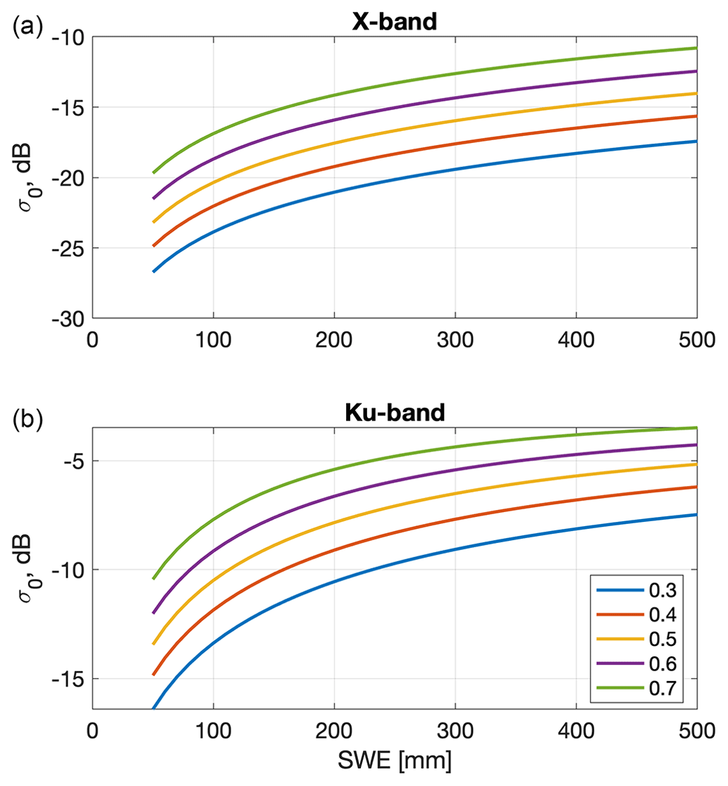
Figure 1The parameterized forward model Mvol(x) illustrating the vv-polarized normalized radar cross section (NRCS) of snow volume backscattering at 40∘ incidence in terms of SWE and ω (values in legend) at 9.2 (a) and 17.9 GHz (b).
The retrieval algorithm is a cost function minimization approach, a legacy algorithm with many years of heritage (Rott et al., 2012). The minimization approach simply identifies the choice of unknowns (i.e., SWE) to minimize a cost function that includes the difference between observed and model-predicted radar backscatter. This section describes the basic formulation of the algorithm, with additional details of how the algorithm is applied for this study (e.g., estimation of ground surface scattering) described in the subsequent section. The algorithm embeds the parameterized forward model presented by Zhu et al. (2021), in which snow volume scattering is parameterized as a function of the SWE and the single-scattering albedo at X-band (ω). A set of empirical equations are used to approximate the full response of radar backscatter to snowpack characteristics derived by the more complex bi-continuous Dense Media Radiative Transfer model of Xu et al. (2012) and Ding et al. (2010). Figure 1 shows the model radar predictions as a function of SWE and ω and shows the rapid increase in backscatter that occurs as snow initially accumulates, as well as the influence of the snow microstructure parametrized by ω.
3.1 Formulation
The cost function minimization approach described here builds from the approach of Zhu et al. (2021). The unknowns SWE and ω are represented as a control vector x, and the parameterized model described above is represented as an operator σ0,mod. In this study, we minimize differences between observations and model predictions in units of decibels [dB], and units of all σ0 quantities are in dB unless otherwise noted. The optimal value of the parameters is computed by minimizing
where σ0,obs is the vector of the volume scattering part of the radar observations, Σobs is the error covariance matrix of the observations, is the vector of the prior estimates of SWE and ω, and Σx is the error covariance of the prior estimates. The parameterized forward model is the sum of the attenuated ground surface scattering and the parameterized volume scattering, but these quantities are additive only in linear units, not in dB; we use an asterisk (“*”) superscript to denote linear quantities. The forward model can be written as
where is the ground surface backscatter, f(x) represents the attenuation of the ground surface backscatter by the snowpack (which depends on SWE and ω in the parameterized model), and is the parameterized snow volume scattering model expressed in linear units. is the backscatter that would be measured from the ground surface in the absence of the snowpack, also referred to as the “background” backscatter.
Following Zhu et al. (2018), we assume that the prior estimate of the single-scattering albedo is either 0.4 or 0.6 in order to indicate whether snowpack is dominated by large scatterers such as depth hoar. We choose using a two-step approach. We first solve the optimization problem,
in which x0 fixes SWE at its prior estimate while ω is allowed to vary. We then set to be either 0.4 or 0.6, depending on which is closer to . Following Zhu et al. (2018), the prior covariance matrix Σx is then assumed diagonal with standard deviation 0.1 for and 50 % of the ERA5-SWE value for .
3.2 Three configurations for estimating prior SWE and ω
We explore three configurations for determining the prior value for SWE () that are then used both in Eq. (1) and in selecting . The first assumes the prior SWE to be equal to the ERA5-Land SWE (SWEERA) at each time step; this is referred to as the “ERA prior” hereafter. The second sets the prior SWE estimate to be equal to the previous SWE retrieval (labeled as ). For the first retrieval of each year, when there is not yet a previous retrieval, the prior SWE is set equal to the ERA5 SWE.
The third configuration uses the weighted average:
where gERA is the weight given to the estimate of SWE from ERA5. The optimal weight can be expressed in terms of the variances of the respective terms:
where the σ terms represent the uncertainty in ERA and the previous SWE estimate, respectively. Assuming that σERA is 50 % of SWEERA and that the uncertainty of is 35 % (accounting for the actual accuracy of the previous retrieval and allowing for the potential of SWE to change between successive retrieval days due to additional precipitation events), then gERA=0.33, which is the value used in what follows. This approach is essentially an optimal weighting between the ERA5 SWE and the previous retrieval; we refer to it as the “weighted average” hereafter. For the first retrieval, when there is not a previous retrieval yet, the prior SWE is set equal to the ERA5 SWE.
For the third configuration, the prior for ω is similarly computed as a weighted average between the ω from the previous retrieval and the ω computed based on the ERA5 SWE, using the same weight as used for SWE, and then classified into either a value of 0.4 or 0.6. In other words, we first compute the prior for time t as described in the last paragraph of Sect. 3.1, which we will refer to as ωERA. We then calculate a weighted average of that value and the previously retrieved ω:
where we use the same weight gERA for ω as used for SWE. Then this value of is used to choose the prior for time t of either 0.4 or 0.6.
4.1 Estimating ground surface scattering
We estimate ground surface scattering independently for each of the 2 years in this study using the ERA5 SWE and early-season backscatter measurements. The early-season backscatter days have a non-zero SWE that is accounted for by solving Eq. (2) for the surface backscatter, for each observation channel, i:
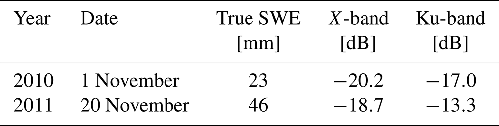
where is the observed backscatter on the day chosen to use for background estimation and xb uses the ERA5 SWE value and ω=0.5 (results were similar for ω between 0.4 and 0.6 due to the low SWE values these times). As shown in Table 1, background NRCS values determined at X-band are fairly consistent between the 2 years, while Ku-band values show larger variations.
Table 1σ0,surf values determined for the 2 years analyzed in this study. True SWE is estimated as described in Sect. 4.2.
4.2 Estimating true SWE
As described in Sect. 2, two in situ SWE datasets are available. Snow pit data are fairly infrequent, covering 36 of the total possible 316 nominal days of the study period (all days from 1 December through 15 March). The automated GWI data cover the entire period but have much higher SWE uncertainty, as they were measured by an experimental sensor (Lemmetyinen et al., 2016a). To obtain daily SWE estimates, we use the simple data assimilation approach described in Appendix A to merge the snow pit and GWI data with a simple snow model driven by precipitation and temperature. These daily SWE estimates agree with snow pit and GWI data when available and also agree with the temperature and precipitation data. The output of the data assimilation is referred to as the “true SWE” hereafter and is used as the basis for evaluating SWE retrievals.
4.3 Flagging wet snow
A small amount of liquid water in the snowpack causes radar backscatter to drop. Throughout the dataset, there are occasional excursions related to the presence of liquid water. We flag these events using the simple but effective wet snow flagging algorithm described in Appendix B. The algorithm has a single parameter: the amount that the data drops in the Ku channel from one day to the next when snow is wet. We do not show the backscatter or snow retrieval data when wet snow is flagged in the main body of the paper (all data are shown in Appendix B), and we do not include the flagged data in assessing algorithm accuracy. See Appendix B for further details on the wet snow flagging algorithm.
4.4 Estimating overall forward model uncertainty
The uncertainty of the observations, Σobs, must also be specified in Eq. (1). There are at least three components that contribute to this uncertainty. The first source is the observations themselves. According to Lemmetyinen et al. (2016a), measurement uncertainty was approximately 1.0 dB, based on repeat measurements of a radar calibration sphere. Examination of the backscatter data, however, clearly shows that the radar measurements are far more precise than 1 dB: e.g., backscatter generally remains stable during the study period between snowfall and melt events. The averaging of the multiple 3 or 4 h radar measurements on each date further reduces this uncertainty. The second source is the parameterized model. Snowpack stratigraphy causes vertical variability in snow scatterers, so that representing layered snowpack backscattering using a single layer parameterized model represents a potential error source that has not been well characterized. The third source of uncertainty lies in the compensation of surface scattering in which σ0,surf is assumed to remain constant throughout the entire winter (Lemmetyinen et al., 2016b). The observation uncertainty Σobs merges all of these sources of uncertainty together.
An analysis was performed to estimate the combined error level. The analysis used the true SWE (described in Sect. 4.2) and the measured backscatter. We compute estimates of true surface scattering following the approach of Sect. 4.1 but using the true SWE to estimate the background scattering, and we also compute optimal estimates of ω. We then evaluate the forward model with the true SWE, true surface scattering, and optimal ω and compare the model predictions with the measured backscatter. This gives an overall estimate of the total uncertainty of the modeling chain. The results showed a combined observational uncertainty of approximately 0.75 dB (16.6 %) across both channels and both years. These values are used in the analysis. We further present sensitivity studies to the observation error in Appendix C.
4.5 Experiments and assessment
Retrievals are performed for each year from 1 December through 15 March in order to exclude periods of predominantly wet snow in both early and late winter. We also artificially introduce additional biases in the ERA5 prior SWE and examine the impact of the retrieved SWE values. Specifically, we multiply the ERA5 prior SWE by a factor of 1+fbias, where fbias ranges from −0.5 to 0.5. The retrieval algorithm has no knowledge of the bias and retains the 50 % assumption for the uncertainty in the prior ERA5 SWE as described in Sect. 3.1. Retrieval accuracy is assessed by both the SWE root mean squared error (RMSE) and the relative RMSE (rRMSE), where the latter is computed by calculating the root mean square of the relative error (i.e., the actual error divided by true SWE) on each day.
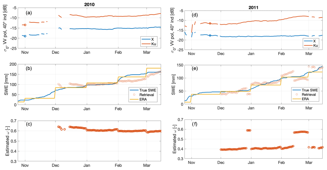
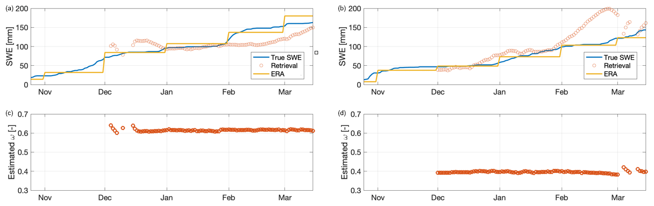
Figure 2For 2010 and 2011, respectively, the observed backscatter (a, d), true, retrieved and prior SWE (b, e), and retrieved ω (c, f) are shown. The circles in panels (a) and (d) show the date selected for characterizing surface scattering for 2010 and 2011, respectively. The results shown here for the prior do not include any artificially imposed bias.
5.1 Results using ERA5 prior
Figure 2 shows the measured backscatter time series, SWE retrieval, true SWE, and prior SWE, and the estimated ω for 2010 and 2011, for the ERA5 prior configuration. In December 2010, the backscatter measurements especially at Ku-band are somewhat erratic, leading to somewhat less accurate retrievals, while in January 2010 the SWE measurements and true SWE are both relatively constant. Snowfall events then increase the SWE in February 2010, while backscatter remains roughly constant, indicating a drop in ω. NRCS values then increase in late February and March, resulting in retrieved SWE values that converge to the true SWE by the end of the study period. The retrieved ω remains near 0.6 throughout the winter. Combining all retrievals across both 2010 and 2011, the ERA5 prior case has rRMSE of 13.7 % and RMSE of 13.8 mm (Table 2).
While this is good performance, the results using this prior configuration are quite sensitive to any bias in the prior. Figure 3 averages performance for 2010 and 2011 and for both negative and positive bias, producing an average response of the algorithm rRMSE to bias. From Fig. 3, the rRMSE for ERA5 increases from 13. % to 46 % as the artificially imposed bias increases from 0 to 0.5. We compute the sensitivity of the rRMSE to the prior as (46 %–13.7 %)/0.5=0.65. Thus, for every 10 % increase in SWE bias, the rRMSE increases by approximately 6.5 %. Thus, the results are quite sensitive to bias in the prior when using the ERA5 data.
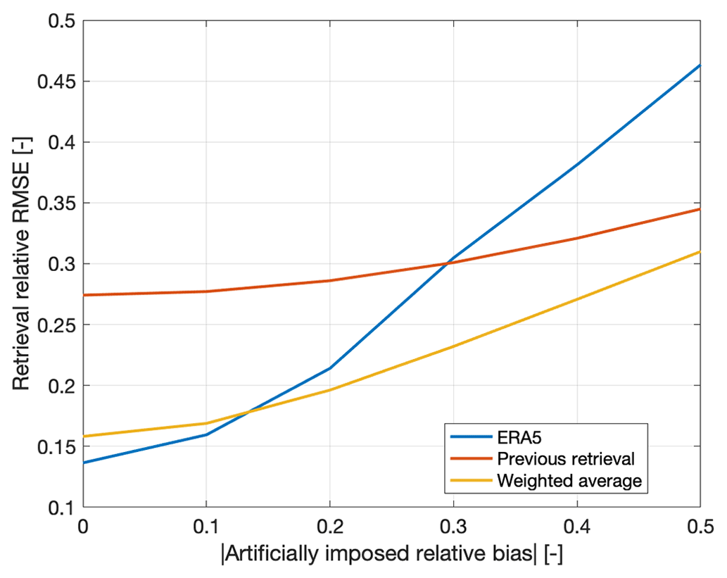
Figure 3Sensitivity of the retrieval relative RMSE to artificially imposed bias on the ERA5 data. These results were obtained by artificially imposing both negative and positive bias and averaging the resulting relative RMSE.
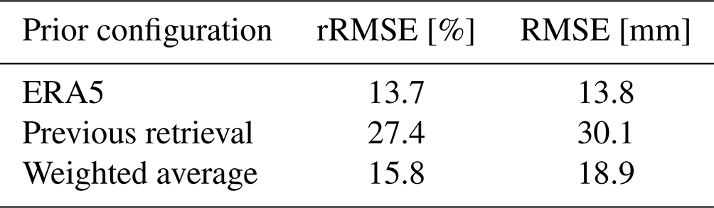
Table 2Average between 2010 and 2011 error statistics for the case without any artificially imposed bias for the cost-minimization algorithm for the ERA5 prior and optimal prior, as described above.
5.2 Results using the previous retrieval prior
Figure 4 shows the SWE and ω retrieval results for the previous retrieval prior. In 2010, results are qualitatively fairly similar to those for the ERA5 prior, although the errors in December are larger, and the SWE retrievals remain more constant in early February. In 2011, the ω retrievals are consistently near 0.4 rather than oscillating between 0.4 and 0.6 in the ERA5 SWE prior. However, the previous retrieval results are more distinct from the ERA5 prior case in February 2011 and show a significant overestimation peaking around 20 February. As the radar backscatter decreases beginning 1 March, the SWE estimates also move back towards the true SWE, and estimates are fairly accurate in March. This divergence in February highlights a weakness of using the previous retrieval approach (and motivates using a weighted average of the previous retrieval and the ERA5 prior SWE, which is presented next). From Table 2, the rRMSE for both years combined is 27.4 %, approximately double that of the ERA5 prior. From Fig. 3, however, we see the great advantage of using the previous retrieval prior configuration: the SWE estimates are nearly insensitive to bias artificially imposed on the prior SWE estimates from ERA5. The rRMSE increases in Fig. 3 from 0.27 to 0.34, a bias sensitivity of 0.14: a 10 % increase in ERA5 prior bias leads to an increase of only 1.4 % in the rRMSE. Thus, the ERA5 prior is relatively accurate but not robust to prior bias, while the previous SWE retrieval is relatively inaccurate but quite robust, further motivating a weighted combination of both.
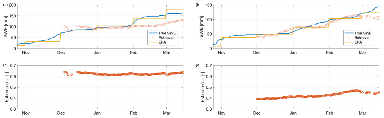
5.3 Results using the weighted average prior
Figure 5 shows the SWE and ω retrieval results for the weighted average prior. The results for 2010 are qualitatively quite similar to those for the previous retrieval prior parameterization. However, the errors in December are noticeably smaller. The results for 2011 are a significant improvement over either the ERA5 prior or the previous retrieval prior. The ω values do not oscillate as they do for the ERA5 prior. Retrievals also show improved performance in February of both years. From Table 2, the rRMSE for both years combined is 15.8 % – far better than the previous retrieval configuration and only marginally larger than the ERA5 prior. From Fig. 3, the sensitivity of the weighted average SWE retrievals similarly lies between the two other configurations. The relative RMSE increases from 15.8 % to 31 %, an increase of just 15.2 % for the bias increasing 50 %, a sensitivity of 0.3. Thus, the weighted average prior represents a compromise between the two other configurations: it has high accuracy but is also relatively insensitive to bias in the ERA5 SWE.
Modern retrieval algorithms often leverage a priori information. When they do so, retrieval algorithms must be shown to be both accurate and relatively insensitive to the a priori information. In this study, we analyze three different configurations for a priori SWE. We show that using the ERA5 prior leads to high retrieval accuracy for this study area but that retrieval results using the ERA5 prior are too sensitive to prior SWE. Thus, using ERA5 or another model alone as a prior is a risky strategy with the algorithm described above. The second configuration uses the previous retrieval instead of ERA5 as the prior. This leads to a very low sensitivity to ERA5 accuracy but a much lower accuracy. This suggested a hybrid approach: we use a weighted average of the ERA5 and the previous SWE, which is a strategy that is both accurate and robust, as shown in Fig. 6.
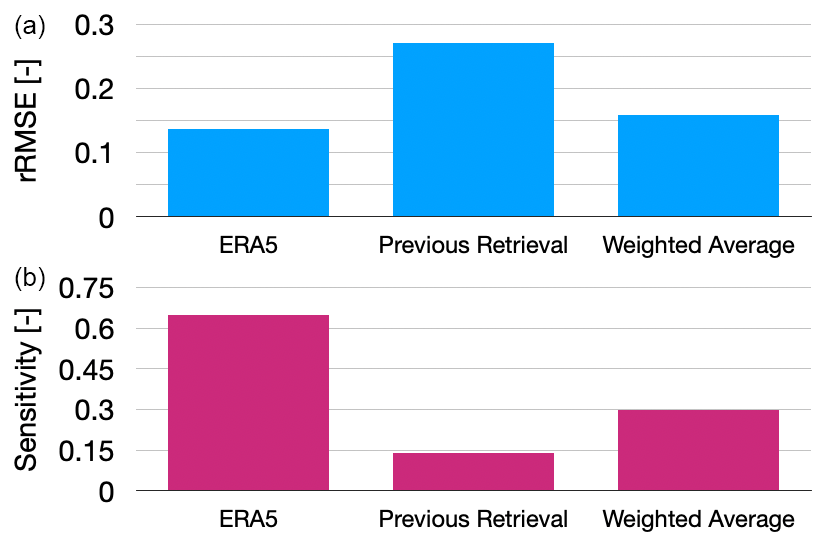
Figure 6Summary of study results: accuracy described by the relative RMSE (a) and sensitivity to the prior estimates of SWE (b) for the three different prior configurations.
Critically, our results show that a highly accurate prior SWE estimate is not necessary to retrieve an accurate SWE retrieval. To further explore these issues, we present a visualization of the retrievals for several of the scenarios where we vary bias systematically. Figure 7a picks two of the many bias scenarios explored in the paper and plots them as time series. First, the figure clarifies the difference between the original ERA5 prior and its 25 % biased time series. Second, the SWE retrieval using only ERA5 (triangle markers) is clearly shown to be highly sensitive to the prior bias. Third, the SWE retrieval using the weighted average of the previous retrieval and ERA5 (circle markers) is seen to be much less sensitive to the prior bias.
Figure 7b shows the absolute value of the SWE error for the prior and the retrieval results for the same scenarios. The error values are the absolute value of the difference between the SWE estimate and the true SWE at each time. Note that in the retrieval using ERA5 prior (red markers), retrieval errors with the biased prior (large markers) are much greater than those with the unbiased prior (small markers). However, in the retrieval using the weighted average (purple markers), retrieval errors with the biased prior are more similar to those with the unbiased prior. Thus, the retrieval using the weighted average prior is much less sensitive to prior bias. We attribute this reduced sensitivity to the use of the previous retrieval in the weighted prior: information about the retrieved SWE is thus transmitted from one time to the next, lessening the importance of having an accurate prior input.
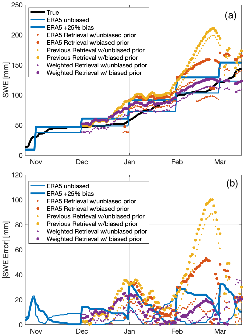
Figure 7Results from the experiments where artificial bias was systematically varied. (a) SWE time series for 2011 at Sodankylä, showing the true SWE computed in the paper (black), the model (ERA5) priors (blue), and the retrievals (circles). The model and retrievals are shown for two of the bias scenarios studied in the paper: no bias and +25 % bias artificially added to the ERA5 model estimates (thin and thick lines, respectively). The retrievals represent three retrieval algorithm configurations (red, gold, and purple for ERA5, previous, and weighted configurations, respectively) for the unbiased scenario (small markers) and scenario with artificial bias added (large markers). (b) Absolute value of the SWE error for the same data and scenarios shown in panel (a); all markers defined the same as in panel (a).
This study helps to show a way forward for satellite mission proposal algorithms. This study does not solve all issues for spaceborne application, especially issues related to forest cover; instead, we focus on benchmarking a simple algorithm that would function well away from the effects of trees. Regarding measurement frequency, we hypothesize that as long as an observation is available since the most recent significant snowfall event, our weighted average algorithm will function with error statistics similar to what are shown here. However, we focus on the daily backscatter measurements here to isolate the issues of surface scattering and the issue of a priori information on SWE and microstructure. Note that the ω values in our study are a proxy for snow microstructure grain size or autocorrelation length (Mätzler, 2002). CoReH2O required a high-precision estimate of snow microstructure grain size (Rott et al., 2012). Our weighted average algorithm avoids that issue by computing a prior estimate of ω from the prior SWE. Prior estimates on SWE are widely available and improving all the time, and our weighted average algorithm has a fairly low sensitivity to the accuracy of the model prior of around 0.3. Thus, a 10 % bias in the modeled SWE leads to only a 3 % increase in relative RMSE. Other studies such as Zhu et al. (2021) and Lemmetyinen et al. (2018) use passive microwave measurements to compute either the rough surface scattering or the microstructure grain size correlation length. However, for spaceborne applications, there would be approximately an order of magnitude difference in the spatial resolution of passive microwave (on the order of kilometers) and radar (on the order of hundreds of meters) measurements, leading to complications. Our approach avoids these issues as well. Finally, the recent study of Pan et al. (2023) shows simultaneous retrieval of SWE and surface scattering using a much more computationally expensive algorithm: approximate differences in compute time are several orders of magnitude. The Pan et al. (2023) approach is likely more accurate than the one shown here but at the cost of being potentially too computationally expensive for a global spaceborne application. Our approach solves the most important issues of resolving sensitivity to prior information and surface scattering while remaining computationally very low cost. Important next steps for this algorithm include testing on datasets from additional sites and working on a simple way to track variations in ω, as described in Appendix D.
This study has applied a previously published algorithm (described by Zhu et al., 2018, and Zhu et al., 2021, and only minimally modified in its application) in order to explore the sensitivity to a priori information using in situ radar measurements. A global model (ERA5) was used to obtain prior estimates of SWE; artificial bias was added to the ERA5 SWE estimates in sensitivity experiments. Surface scattering and single-scatter albedo ω were treated in objective ways based on published literature requiring no other external or a priori information. We explored three configurations for prior information which uses the ERA5 alone, the previous retrieval, and a weighted average of the two, respectively. Using ERA5 alone confirms a problem identified in previous studies: the ERA5 prior SWE must be relatively accurate in order to achieve successful SWE retrievals. However, using the weighted combination of ERA5 and the previous retrieval greatly diminishes the dependence on prior information. This configuration achieved an accuracy of 15.8 % relative RMSE and increased only 3 % per 10 % increase in prior bias.
The algorithm presented meets reasonable accuracy requirements, has been shown to be robust to bias in the input prior measurements, and is feasible for implementation in satellite measurements using existing prior datasets. Future work should explore new algorithms employing simple state-space models to track changes in ω and SWE while preserving the overall simplicity of the approach. These results are limited to shallow snow on flat terrain, with a homogenous footprint, and no attenuation of the radar measurements by forests. Nonetheless, this study greatly allays a major concern in retrieval of SWE from radar backscatter: the need for accurate prior information. These findings should build confidence in the community that current proposals for future satellite missions will be able to deliver accurate estimates of SWE (Tsang et al., 2022).
As described in Sect. 2.2 and 2.3, there is no perfect estimate of daily SWE: the snow pit data are relatively infrequent, but the gamma SWE measurements are relatively imprecise. We apply a two-step process to obtain a daily combined SWE estimate. In the first step, we use both snow pit and gamma data to calibrate a simple temperature index snow model forced by precipitation and air temperature measurements described in Sect. 2.4. In the second step, we derive a new estimate via an optimization algorithm, informed by both the data themselves and the calibrated model. This true SWE has superior agreement with all available snow pit and gamma data, is informed by snowfall timing and air temperature, and is available daily.
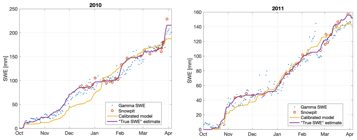
Figure A1Estimates of gamma SWE, snow pit SWE, the calibrated model, and true SWE for 2010 and 2011.
In the first step, we calibrate the temperature index model of Slater et al. (2013) using both snow pit and gamma SWE observations. The snow model has a total of five parameters, including a constant multiplicative gage undercatch parameter, air temperature discriminating rainfall from snowfall, and three parameters governing snowmelt. The model is computed one “water year” at a time, beginning 1 October and running through 30 September, at a daily time step. The calibration objective function measures the mismatch between model predictions and in situ snow observations, weighted by the respective uncertainty of each observation type. Here we assume snow pit SWE to have 15 mm uncertainty and gamma SWE to have 30 mm uncertainty. This model calibration also results in a calibrated estimate of snowfall and snowmelt. The result of the calibration step are SWE simulations that match both pits and gamma SWE to reasonable precision but neglect any factors not in the model, such as sublimation or storm-specific errors in precipitation measurement.
In the second step, we compute the true SWE formulated as an optimization problem. We compute an estimate of snowfall, melt, and SWE subject to the constraint of mass balance at each step, with the objective function penalizing differences from the model calibrated estimates of snowfall and snowmelt, and also from the snow pit SWE. We add further constraints disallowing snowfall (and thus increase in SWE) when there is no measured precipitation and disallowing snowmelt (and thus decrease in SWE) when there is no model calibrated snowmelt.
Table A1Difference statistics between gamma SWE and true SWE: mean and root mean square of the difference and relative difference between gamma and true SWE.
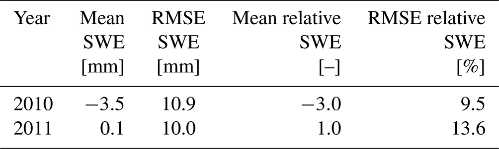
Figure A1 shows the optimal true SWE estimates, along with snow pit, gamma, and calibrated model SWE. The calibrated model sometimes tracks the SWE well and sometimes does not, presumably due to time-varying errors in the precipitation undercatch. The gamma SWE sometimes differs by tens of millimeters (mm) from the true SWE estimate, and at other times it is significantly different from the snow pit measurements, such as in February 2010 and February 2011. Table A1 shows that the relative root mean square (rms) differences between the gamma SWE and the true SWE estimate are 9.5 % in 2010 and 13.6 in 2011; these errors are of the same order of magnitude as the retrieval errors cited throughout the study. The true SWE estimate integrates all information into a single estimate and thus is used as the reference with which to compare SWE retrievals throughout the study.
The overall wet snow flag strategy in this paper is to attempt to show results only for dry snow. Thus, our intent is not to develop and verify an objective wet snow algorithm that can be used in other contexts. From Fig. B1, some data points contain sharp drops in backscatter. Most of these occur early in the season, but in 2011, some of them occur in March. The presence of wet snow and these sharp drops in backscatter complicates attempts to identify the surface scattering as well as to estimate SWE.
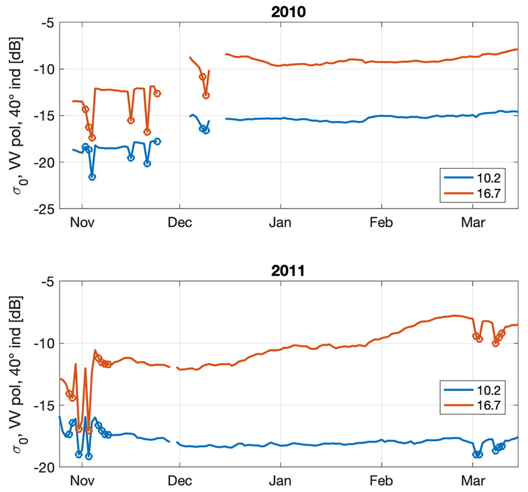
Figure B1The radar data at X- and Ku-band are shown. Data points flagged as wet snow are shown as circles.
We analyzed these sharp drops for the Ku-band data and found that they represent changes greater than 0.5 dB. We use sharp changes in radar backscatter to compute a wet snow flag. The wet snow flag is set to “true” if the algorithm identifies wet snow for day t.
For the case where the flag is set to “false” on day t−1, if the decrease in backscatter from day t−1 to day t is greater than 0.5 dB, then we set the flag to “true” for day t.
For the case where the flag is set to “true” on day t−1, if the increase in backscatter from day t−1 to day t is greater than 0.5 dB, then we set the flag to “false” for day t.
In other words, the flag stays set as it was on the previous day, unless a sharp change in backscatter causes the flag to change. This simple algorithm identified all of the obviously wet snow in the dataset, failing in only one period of the dataset. In November 2011, the transition from wet snow to dry snow was a gradual increase in backscatter rather than a sharp rise. We thus added a condition that if the flag stays set at “true” for 3 consecutive days, we change the flag status to “false”.
Further work on more objective and widely applicable algorithms to flag wet snow should be developed. This approach allows us to remove apparently wet snow data from the analysis and is thus well suited to this study.
How accurately can the parameterized model explain the measured backscatter data? This question can be addressed (though not definitively answered) by analyzing the model residuals using the true SWE, the true estimates of surface scattering, and the optimal estimates of ω.
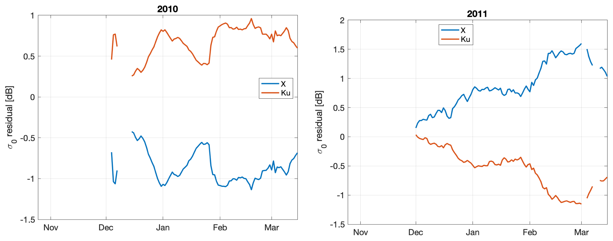
Figure C1Model residuals using true SWE, true surface scattering, and optimal ω for 2010 and 2011.
In both years, the residuals are dominated by bias for both channels: in 2010, the Ku residual is always positive and the X residual is always negative; the converse is true in 2011. Nearly all of the overall rms error in both channels and both years is composed of bias (Table C1). The average rms error for both years and both channels is 0.8 dB.
Table C1Model residual errors: mean (i.e., bias), standard deviation (SD), and root mean square (rms) for X and Ku and for both years.
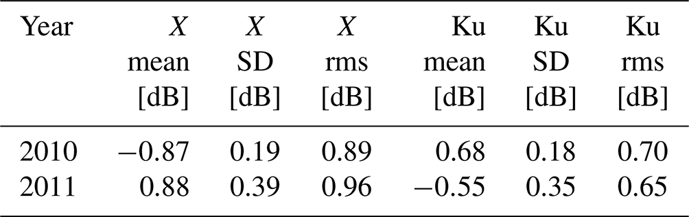
Table C2Sensitivity of relative rms SWE errors [%] for the weighted average prior configuration to the specified observation uncertainty standard deviations used in the measurement error covariance matrix Σobs.
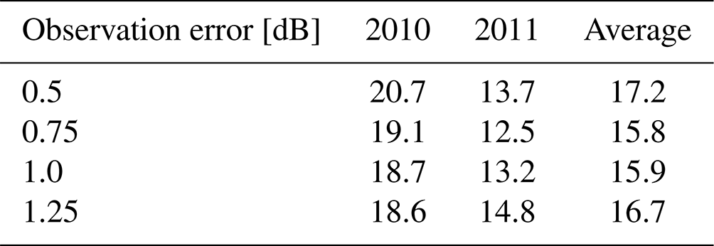
From the point of view of SWE retrieval, the practical question is what values of Σobs to use in the cost function (Eq. 1). Table C2 shows that the rms errors that are mostly analyzed in this study are relatively insensitive to the specified observation errors in Σobs.
Despite the weighted average algorithm successfully achieving a reasonably high accuracy and low sensitivity to bias, room for improvement remains. For example, Fig. 5 shows that the retrieval does not capture the increase in SWE in February 2010. To further investigate the performance of the weighted average approach, we analyzed the optional ω estimates, i.e., values of ω that minimize the difference between the parameterized model evaluated at the true SWE. To do this, we additionally calculate a true surface scattering estimate, using the true SWE in Eq. (7). Using the true surface scattering, true SWE, and observations, we calculate the optimal ω by minimizing the cost function, Eq. (3).
Figure D1 shows the estimates of optimal ω for both years. In 2010, we see drops in ω near the end of December and the end of January that correspond to increases in SWE, i.e., snowfall events. This dynamic has a simple physical explanation. We assume that ω is a metric that can be related to snow microstructure such as a characteristic length scale like the autocorrelation length (L) (Mätzler, 2002). As snow ages, L increases due to vapor flux transport as shown in Flanner and Zender (2006). A snowfall event would typically combine new snowfall with smaller L with snowpack with larger L and thus would have the net effect of reducing the combined L, as described by Durand and Margulis (2006) and Li et al. (2015). This simple conceptual model explains the lack of change in the measured radar backscatter, e.g., in early February 2010: SWE increases, but a corresponding decrease in ω cancels any change in measured backscatter. This conceptual model explains 2011 data as well: snowfall events throughout the month of January lead to a gradual increase in SWE, corresponding with very little change in measured backscatter and thus a gradual drop in ω. Similarly, snowfall events in late February and early March 2011 are accompanied by a drop in measured backscatter, leading to a drop in estimated ω. Thus, the initially counterintuitive behavior that measured backscatter does not correspond with snowfall events is simply explained by drops in ω due to new snowfall.
Figure D1 also shows that increases in measured backscatter occur during periods when SWE is relatively constant. This is consistent with the fact that increases in L drive changes in measured backscatter. In 2010, SWE is fairly constant from mid-February to early March, a period where ω increases gradually, along with the measured backscatter. In 2011, SWE is constant in December but measured backscatter increases, leading to a corresponding increase in ω. Similarly, ω increases throughout February, as SWE stays constant and measured backscatter increases throughout the month. This is broadly similar to behavior noticed in simulated brightness temperature over short spatial distances, in terms of tradeoffs between SWE and microstructure correlation length Rutter et al. (2014). Thus, the initially counterintuitive behavior that measured backscatter increases in periods when SWE is constant is simply explained by increases in ω due to increasing L due to well-understood microphysical processes.
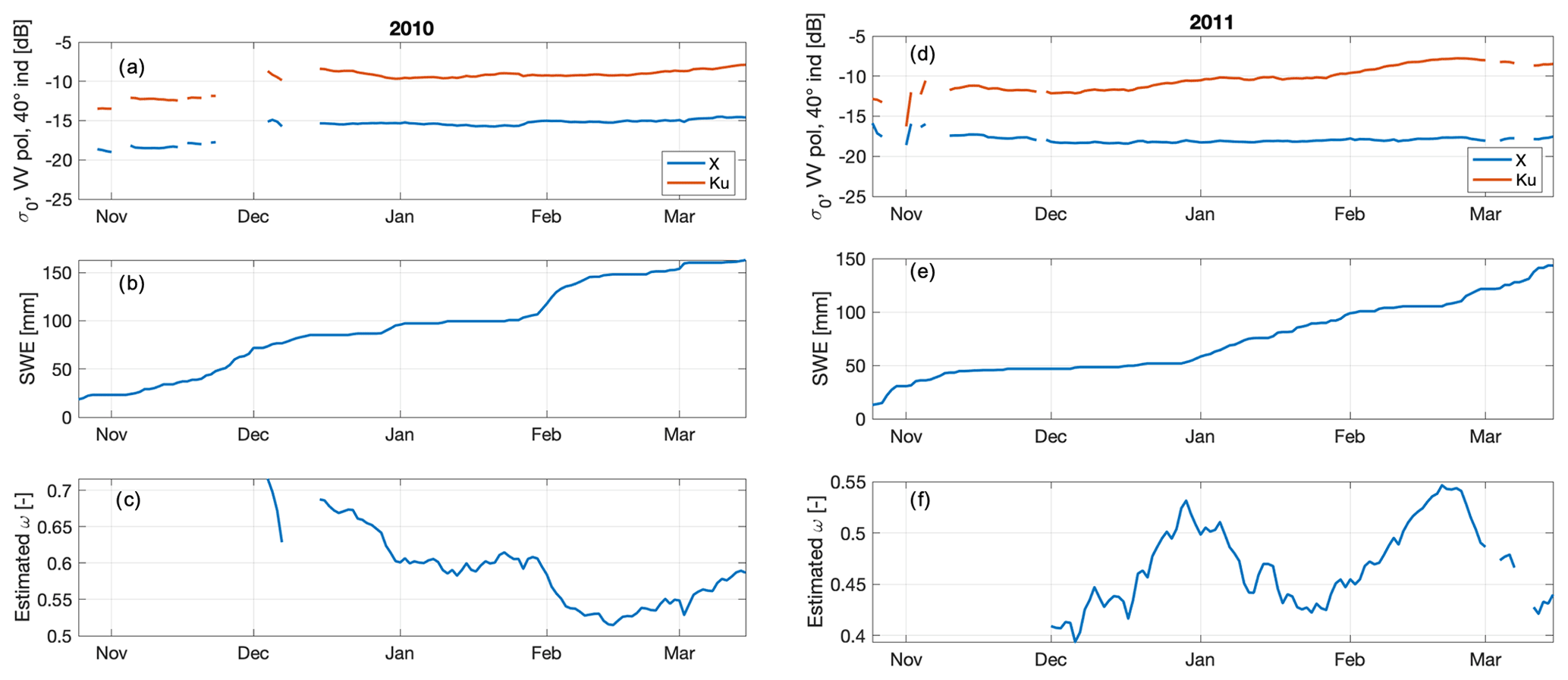
Figure D1Optimal estimates of single-scattering albedo (ω), computed as described in the text (c, f) for 2010 and 2011, respectively, along with radar backscatter observations and true SWE.
All data are from the NoSREx campaign or ERA5: see Lemmetyinen et al. (2016a) or Hersbach et al. (2020), respectively.
MD wrote the paper and performed most of the analyses. JD performed some of the analyses. JTJ and EJK advised on the study and edited the paper. LT and FB provided the parameterized model, advised on the study, and edited the paper.
The contact author has declared that none of the authors has any competing interests.
Publisher’s note: Copernicus Publications remains neutral with regard to jurisdictional claims made in the text, published maps, institutional affiliations, or any other geographical representation in this paper. While Copernicus Publications makes every effort to include appropriate place names, the final responsibility lies with the authors.
This research has been supported by the NASA Terrestrial Hydrology Program under grant agreement number 80NSSC17K0200.
This paper was edited by Melody Sandells and reviewed by two anonymous referees.
Cui, Y., Xiong, C., Lemmetyinen, J., Shi, J., Jiang, L., Peng, B., Li, H., Zhao, T., Ji, D., and Hu, T.: Estimating Snow Water Equivalent with Backscattering at X and Ku Band Based on Absorption Loss, Remote Sens.-Basel, 8, 505, https://doi.org/10.3390/rs8060505, 2016. a, b
Ding, K.-H., Xu, X., and Tsang, L.: Electromagnetic Scattering by Bicontinuous Random Microstructures with Discrete Permittivities, IEEE T. Geosci. Remote, 48, 3139–3151, https://doi.org/10.1109/tgrs.2010.2043953, 2010. a
Durand, M. and Margulis, S. A.: Feasibility Test of Multifrequency Radiometric Data Assimilation to Estimate Snow Water Equivalent, J. Hydrometeorol., 7, 443–457, https://doi.org/10.1175/jhm502.1, 2006. a
Durand, M., Gleason, C. J., Pavelsky, T. M., Frasson, R. P. d. M., Turmon, M., David, C. H., Altenau, E. H., Tebaldi, N., Larnier, K., Monnier, J., Malaterre, P. O., Oubanas, H., Allen, G. H., Astifan, B., Brinkerhoff, C., Bates, P. D., Bjerklie, D., Coss, S., Dudley, R., Fenoglio, L., Garambois, P., Getirana, A., Lin, P., Margulis, S. A., Matte, P., Minear, J. T., Muhebwa, A., Pan, M., Peters, D., Riggs, R., Sikder, M. S., Simmons, T., Stuurman, C., Taneja, J., Tarpanelli, A., Schulze, K., Tourian, M. J., and Wang, J.: A Framework for Estimating Global River Discharge From the Surface Water and Ocean Topography Satellite Mission, Water Resour. Res., 59, e2021WR031614, https://doi.org/10.1029/2021wr031614, 2023. a
Flanner, M. G. and Zender, C. S.: Linking snowpack microphysics and albedo evolution, J. Geophys. Res.-Atmos., 111, D12208, https://doi.org/10.1029/2005jd006834, 2006. a
Hersbach, H., Bell, B., Berrisford, P., Hirahara, S., Horányi, A., Muñoz‐Sabater, J., Nicolas, J., Peubey, C., Radu, R., Schepers, D., Simmons, A., Soci, C., Abdalla, S., Abellan, X., Balsamo, G., Bechtold, P., Biavati, G., Bidlot, J., Bonavita, M., Chiara, G., Dahlgren, P., Dee, D., Diamantakis, M., Dragani, R., Flemming, J., Forbes, R., Fuentes, M., Geer, A., Haimberger, L., Healy, S., Hogan, R. J., Hólm, E., Janisková, M., Keeley, S., Laloyaux, P., Lopez, P., Lupu, C., Radnoti, G., Rosnay, P., Rozum, I., Vamborg, F., Villaume, S., and Thépaut, J.: The ERA5 global reanalysis, Q. J. Roy. Meteor. Soc., 146, 1999–2049, https://doi.org/10.1002/qj.3803, 2020. a, b, c
King, J., Derksen, C., Toose, P., Langlois, A., Larsen, C., Lemmetyinen, J., Marsh, P., Montpetit, B., Roy, A., Rutter, N., and Sturm, M.: The influence of snow microstructure on dual-frequency radar measurements in a tundra environment, Remote Sens. Environ., 215, 242–254, https://doi.org/10.1016/j.rse.2018.05.028, 2018. a
Lemmetyinen, J., Kontu, A., Pulliainen, J., Vehviläinen, J., Rautiainen, K., Wiesmann, A., Mätzler, C., Werner, C., Rott, H., Nagler, T., Schneebeli, M., Proksch, M., Schüttemeyer, D., Kern, M., and Davidson, M. W. J.: Nordic Snow Radar Experiment, Geosci. Instrum. Method. Data Syst., 5, 403–415, https://doi.org/10.5194/gi-5-403-2016, 2016a. a, b, c, d, e, f, g, h
Lemmetyinen, J., Schwank, M., Rautiainen, K., Kontu, A., Parkkinen, T., Mätzler, C., Wiesmann, A., Wegmüller, U., Derksen, C., Toose, P., Roy, A., and Pulliainen, J.: Snow density and ground permittivity retrieved from L-band radiometry: Application to experimental data, Remote Sens. Environ., 180, 377–391, https://doi.org/10.1016/j.rse.2016.02.002, 2016b. a
Lemmetyinen, J., Derksen, C., Rott, H., Macelloni, G., King, J., Schneebeli, M., Wiesmann, A., Leppänen, L., Kontu, A., and Pulliainen, J.: Retrieval of Effective Correlation Length and Snow Water Equivalent from Radar and Passive Microwave Measurements, Remote Sens.-Basel, 10, 170, https://doi.org/10.3390/rs10020170, 2018. a
Lemmetyinen, J., Ruiz, J. J., Cohen, J., Haapamaa, J., Kontu, A., Pulliainen, J., and Praks, J.: Attenuation of Radar Signal by a Boreal Forest Canopy in Winter, IEEE Geosci. Remote S., 19, 1–5, https://doi.org/10.1109/lgrs.2022.3187295, 2022. a
Li, D., Durand, M., and Margulis, S. A.: Large-Scale High-Resolution Modeling of Microwave Radiance of a Deep Maritime Alpine Snowpack, IEEE T. Geosci. Remote, 53, 2308–2322, https://doi.org/10.1109/tgrs.2014.2358566, 2015. a
Mortimer, C., Mudryk, L., Derksen, C., Luojus, K., Brown, R., Kelly, R., and Tedesco, M.: Evaluation of long-term Northern Hemisphere snow water equivalent products, The Cryosphere, 14, 1579–1594, https://doi.org/10.5194/tc-14-1579-2020, 2020. a
Mätzler, C.: Relation between grain-size and correlation length of snow, J. Glaciol., 48, 461–466, https://doi.org/10.3189/172756502781831287, 2002. a, b, c
Pan, J., Durand, M., Lemmetyinen, J., Liu, D., and Shi, J.: Snow water equivalent retrieved from X- and dual Ku-band scatterometer measurements at Sodankylä using the Markov Chain Monte Carlo method, The Cryosphere Discuss. [preprint], https://doi.org/10.5194/tc-2023-85, in review, 2023. a, b, c
Picard, G., Löwe, H., Domine, F., Arnaud, L., Larue, F., Favier, V., Meur, E. L., Lefebvre, E., Savarino, J., and Royer, A.: The Microwave Snow Grain Size: A New Concept to Predict Satellite Observations Over Snow-Covered Regions, AGU Advances, 3, e2021AV000630, https://doi.org/10.1029/2021av000630, 2022. a
Rott, H., Duguay, C., Etchevers, P., Essery, R., Hajnsek, I., Macelloni, G., Malnes, E., and Pulliainen, J.: CoReH2O Report for mission selection: An Earth Explorer to observe snow and ice, Tech. rep., European Space Agency, https://earth.esa.int/eogateway/documents/20142/37627/CoReH2O-Report-for-Mission-Selection-An-Earth-Explorer-to-observe-snow-and-ice.pdf (last access: 13 December 2023), 2012. a, b, c, d
Rutter, N., Sandells, M., Derksen, C., Toose, P., Royer, A., Montpetit, B., Langlois, A., Lemmetyinen, J., and Pulliainen, J.: Snow stratigraphic heterogeneity within ground-based passive microwave radiometer footprints: Implications for emission modeling, J. Geophys. Res.-Earth, 119, 550–565, https://doi.org/10.1002/2013jf003017, 2014. a
Rutter, N., Sandells, M. J., Derksen, C., King, J., Toose, P., Wake, L., Watts, T., Essery, R., Roy, A., Royer, A., Marsh, P., Larsen, C., and Sturm, M.: Effect of snow microstructure variability on Ku-band radar snow water equivalent retrievals, The Cryosphere, 13, 3045–3059, https://doi.org/10.5194/tc-13-3045-2019, 2019. a, b
Sandells, M., Lowe, H., Picard, G., Dumont, M., Essery, R., Floury, N., Kontu, A., Lemmetyinen, J., Maslanka, W., Morin, S., Wiesmann, A., and Matzler, C.: X-Ray Tomography-Based Microstructure Representation in the Snow Microwave Radiative Transfer Model, IEEE T. Geosci. Remote, 60, 1–15, https://doi.org/10.1109/tgrs.2021.3086412, 2021. a, b
Slater, A. G., Barrett, A. P., Clark, M. P., Lundquist, J. D., and Raleigh, M. S.: Uncertainty in seasonal snow reconstruction: Relative impacts of model forcing and image availability, Adv. Water Resour., 55, 165–177, https://doi.org/10.1016/j.advwatres.2012.07.006, 2013. a
Tsang, L., Durand, M., Derksen, C., Barros, A. P., Kang, D.-H., Lievens, H., Marshall, H.-P., Zhu, J., Johnson, J., King, J., Lemmetyinen, J., Sandells, M., Rutter, N., Siqueira, P., Nolin, A., Osmanoglu, B., Vuyovich, C., Kim, E., Taylor, D., Merkouriadi, I., Brucker, L., Navari, M., Dumont, M., Kelly, R., Kim, R. S., Liao, T.-H., Borah, F., and Xu, X.: Review article: Global monitoring of snow water equivalent using high-frequency radar remote sensing, The Cryosphere, 16, 3531–3573, https://doi.org/10.5194/tc-16-3531-2022, 2022. a, b, c
Ulaby, F. T. and Long, D. G.: Microwave Radar and Radiometric Remote Sensing, The University of Michigan Press, Ann Arbor, 2014. a
Xu, X., Tsang, L., and Yueh, S.: Electromagnetic Models of Co/Cross Polarization of Bicontinuous/DMRT in Radar Remote Sensing of Terrestrial Snow at X- and Ku-band for CoReH2O and SCLP Applications, IEEE J. Sel. Top. Appl., 5, 1024–1032, https://doi.org/10.1109/jstars.2012.2190719, 2012. a, b
Zhu, J., Tan, S., King, J., Derksen, C., Lemmetyinen, J., and Tsang, L.: Forward and Inverse Radar Modeling of Terrestrial Snow Using SnowSAR Data, IEEE T. Geosci. Remote, 56, 7122–7132, https://doi.org/10.1109/tgrs.2018.2848642, 2018. a, b, c, d, e, f, g
Zhu, J., Tan, S., Tsang, L., Kang, D., and Kim, E.: Snow Water Equivalent Retrieval Using Active and Passive Microwave Observations, Water Resour. Res., 57, e2020WR027563, https://doi.org/10.1029/2020wr027563, 2021. a, b, c, d, e, f, g, h, i, j
Zhu, J., Tsang, L., Liao, T.-H., Johnson, J. T., Kang, D. H., and Kim, E. J.: Radar Backscattering of Rough Soil Surfaces From L-Band to Ku-Band With NMM3D, IEEE Geosci. Remote S., 19, 1–5, https://doi.org/10.1109/lgrs.2022.3188702, 2022. a
- Abstract
- Introduction
- Datasets and study area
- Retrieval algorithm formulation and application
- Experiment design
- Results
- Discussion
- Conclusions
- Appendix A: Estimating true SWE
- Appendix B: Wet snow flagging
- Appendix C: Analysis of observation error
- Appendix D: Analyzing optimal ω estimates
- Data availability
- Author contributions
- Competing interests
- Disclaimer
- Financial support
- Review statement
- References