Modeling the timing of Patagonian Ice Sheet retreat in the Chilean Lake District from 22–10 ka

Studying the retreat of the Patagonian Ice Sheet (PIS) during the last deglaciation represents an important opportunity to understand how ice sheets outside the polar regions have responded to deglacial changes in temperature and large-scale atmospheric circulation. At the northernmost extension of the PIS during the Last Glacial Maximum (LGM), the Chilean Lake District (CLD) was influenced by the southern westerly winds (SWW), which strongly modulated the hydrologic and heat budgets of the region. Despite progress in constraining the nature and timing of deglacial ice retreat across this area, considerable uncertainty in the glacial history still exists due to a lack of geologic constraints on past ice margin change. Where the glacial chronology is lacking, ice sheet models can provide important insight into our understanding of the characteristics and drivers of deglacial ice retreat. Here we apply the Ice Sheet and Sea-level System Model (ISSM) to simulate the LGM and last deglacial ice history of the PIS across the CLD at high spatial resolution (450 m). We present a transient simulation of ice margin change across the last deglaciation using climate inputs from the National Center for Atmospheric Research Community Climate System Model (CCSM3) Trace-21ka experiment. At the LGM, the simulated ice extent across the CLD agrees well with the most comprehensive reconstruction of PIS ice history (PATICE). Coincident with deglacial warming, ice retreat ensues after 19 ka, with large-scale ice retreat occurring across the CLD between 18 and 16.5 ka. By 17 ka, the northern portion of the CLD becomes ice free, and by 15 ka, ice only persists at high elevations as mountain glaciers and small ice caps. Our simulated ice history agrees well with PATICE for early deglacial ice retreat but diverges at and after 15 ka, where the geologic reconstruction suggests the persistence of an ice cap across the southern CLD until 10 ka. However, given the high uncertainty in the geologic reconstruction of the PIS across the CLD during the later deglaciation, this work emphasizes a need for improved geologic constraints on past ice margin change. While deglacial warming drove the ice retreat across this region, sensitivity tests reveal that modest variations in wintertime precipitation (∼10 %) can modulate the pacing of ice retreat by up to 2 ka, which has implications when comparing simulated outputs of ice margin change to geologic reconstructions. While we find that TraCE-21ka simulates large-scale changes in the SWW across the CLD that are consistent with regional paleoclimate reconstructions, the magnitude of the simulated precipitation changes is smaller than what is found in proxy records. From our sensitivity analysis, we can deduce that larger anomalies in precipitation, as found in paleoclimate proxies, may have had a large impact on modulating the magnitude and timing of deglacial ice retreat. This fact highlights an additional need for better constraints on the deglacial change in strength, position, and extent of the SWW as it relates to understanding the drivers of deglacial PIS behavior.

1 Introduction

During the Last Glacial Maximum (LGM), the Patagonian Ice Sheet (PIS) covered the Andes Mountains from 38 to 55° S with an estimated sea-level equivalent ice volume of 1.5 m (Davies et al., 2020). The behavior of the ice and the related climate forcings from the LGM to the deglacial period at the northernmost extent of the PIS, across an area presently known as the Chilean Lake District (CLD: 37–41.5° S), have been subjects of historical interest (Mercer, 1972; Porter, 1981; Lowell et al., 1995; Andersen et al., 1999; Denton et al., 1999; Glasser et al., 2008; Moreno et al., 2015; Kilian and Lamy, 2012; Lamy et al., 2010) and have served as important constraints towards understanding the drivers of ice sheet change across centennial to millennial timescales. Currently, PATICE (Davies et al., 2020) serves as the latest and most complete reconstruction of the entire PIS during the LGM and last deglaciation. Across the CLD (Fig. 1), the LGM ice limits are only well constrained by terminal moraines in the southwest and western margins (Denton et al., 1999; Glasser et al., 2008, Moreno et al., 2015). However, due to a lack of geomorphological and geochronologic constraints on ice margin change following the LGM, the reconstructed deglaciation remains highly uncertain.

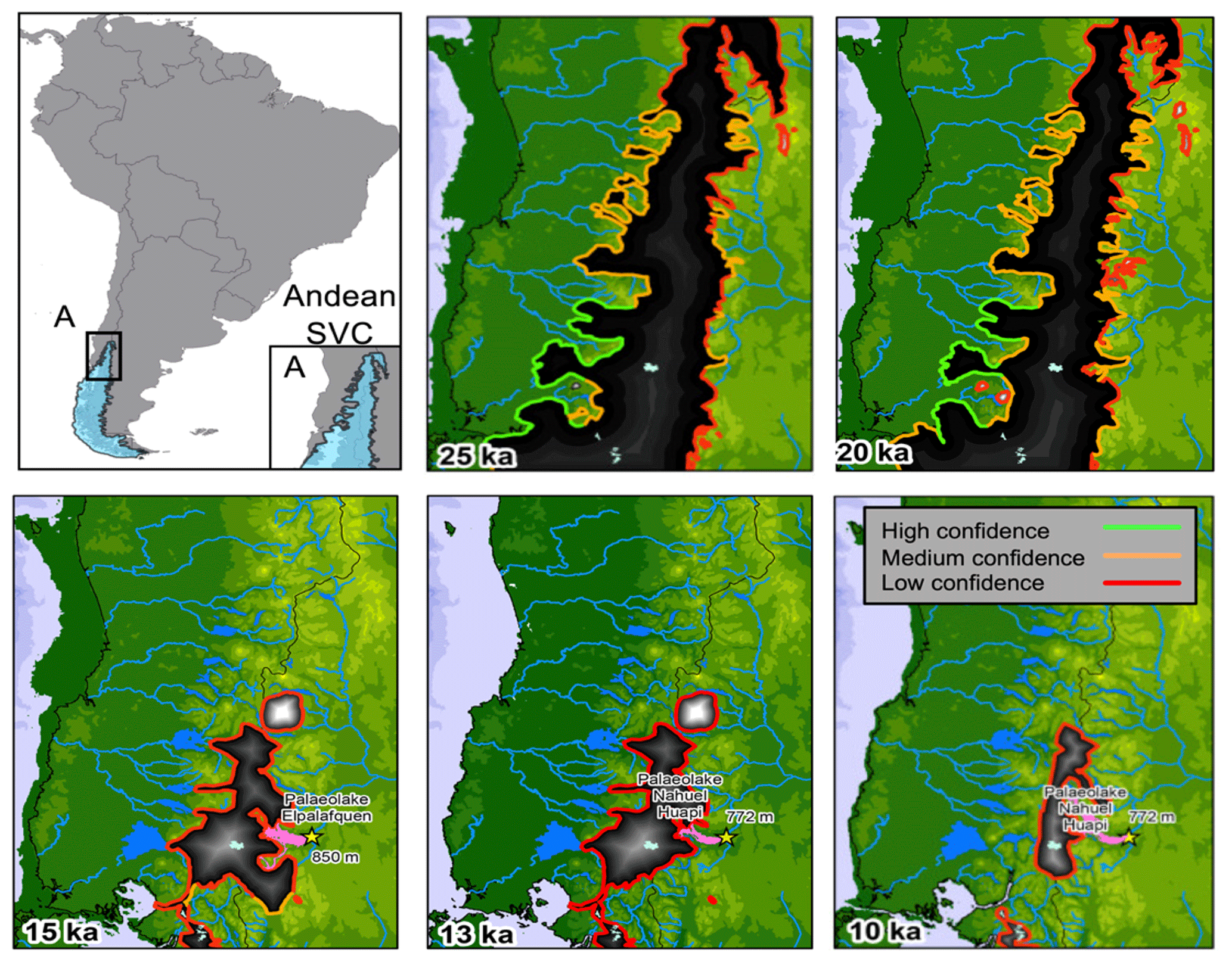
Figure 1 Location of the study area across the Chilean Lake District (CLD; upper left panel). The reconstructed ice extents from PATICE for the PIS across the CLD at 25, 20, 15, 13, and 10 ka are taken from Davies et al. (2020). The color of the line marking the reconstructed ice extent corresponds to the confidence in the reconstruction, as described in Sect. 3.3.

While deglacial warming was a primary driver of ice retreat across the CLD, evidence suggests that variations in precipitation patterns influenced the timing and magnitude of this retreat (Moreno et al., 1999; Rojas et al., 2009). The wintertime climate across South America is strongly influenced by the southern annular mode (SAM; Hartmann and Lo, 1998), the phase and strength of which are regulated by changes in the difference in zonal mean sea-level pressure between middle (40° S) and high latitudes (65° S). The SAM in turn modulates the strength and position of the southern westerly winds (SWW) over decadal to multi-centennial timescales, with the SWW exerting considerable control over the synoptic-scale hydrologic and heat budgets (Garreaud et al., 2013). Paleoclimate data indicate that the position, strength, and extent of the SWW varied latitudinally during the LGM and last deglaciation: it migrated southward during warmer intervals and northward during cooler intervals, ultimately altering the overall ice sheet mass balance (Mercer, 1972; Denton et al., 1999; Lamy et al., 2010; Kilian and Lamy, 2012; Boex et al., 2013). Terrestrial paleoclimate proxies that indicate that the CLD was wetter during the LGM and early deglaciation period have been used to support the idea that the SWW migrated northward of 41° S across the CLD (Moreno et al., 1999, 2015, 2018; Diaz et al., 2023). Additionally, these proxies indicate a switch from hyperhumid to humid conditions around 17 300 cal yr  BP, which was inferred by Moreno et al. (2015) as indicating the poleward migration of the SWW south of the CLD.

However, inferring changes in the SWW across the last deglaciation from paleoclimate proxies can be problematic, as outlined by Kohfeld et al. (2013), who compiled an extensive dataset of paleoclimate archives that record changes in moisture, precipitation–evaporation balance, ice accumulation, runoff and precipitation, dust deposition, marine indicators of sea surface temperature, ocean fronts, and biologic productivity. Kohfeld et al. (2013) conclude that environmental changes inferred from existing paleoclimate data could potentially be explained by a range of plausible scenarios for the state of and change in the SWW during the LGM and last deglaciation, such as a strengthening, poleward or equatorward migration, or no change. Climate model results from Sime et al. (2013) indicate that the reconstructed changes in moisture from Kohfeld et al. (2013) can be simulated well without invoking large shifts or changes in strength of the SWW. This discrepancy also exists amongst climate models, which diverge on whether the LGM SWW was shifted equatorward or poleward and was stronger or weaker than in the present day (Togweiler et al., 2006; Menviel et al., 2008; Rojas et al., 2009; Rojas, 2013; Sime et al., 2013; Jiang and Yan, 2020). Therefore, we still do not have a firm understanding from paleoclimate proxies and climate models of how the SWW may have changed during the last deglaciation and how these variations may have influenced the deglaciation of the PIS.

Early paleo-ice-sheet modeling experiments across the PIS have focused on evaluating the relationship between the simulated LGM ice sheet geometry in response to a spatially uniform temperature change (Hulton et al., 2002; Sugden et al., 2002; Hubbard et al., 2005). While those early simulations provided constraints on PIS areal extent, ice volume, and sensitivity to LGM temperature depressions, the spatially varying temperature and precipitation were not considered. Recently, Yan et al. (2022) simulated the PIS behavior at the LGM using an ensemble of climate model output from the Paleoclimate Modelling Intercomparison Project (PMIP4; Kageyama et al., 2021). Results that best match the empirical reconstructions from PATICE (Davies et al., 2020) suggest that a reduction in temperature was likely the main driver of PIS LGM extent, although the authors found that variation in the regional LGM precipitation anomaly can have large impacts on the simulated ice sheet geometry. This evidence is supported by recent glacier modeling across the northeastern Patagonian Andes which suggests that increases in precipitation during the termination of the LGM are necessary for the model to fit the reconstructed glacier extent (Muir et al., 2023; Leger et al., 2021b). Additionally, Martin et al. (2022) found that precipitation greater than that in the present day is needed to explain the late glacial and Holocene readvance of the Monte San Lorenzo ice cap lying to the southeast of the current Northern Patagonian Ice Field. These regional studies therefore provide further evidence that late glacial and deglacial variability in precipitation, perhaps driven by changes in the SWW, influenced PIS retreat and readvance over numerous timescales.

To advance our understanding of the last glacial and deglacial ice behavior across the CLD, we use a numerical ice sheet model to simulate the LGM ice geometry and deglacial ice retreat using transiently evolving boundary conditions from a climate model simulation of the last 21 000 years (TraCE-21ka; Liu et al., 2009; He et al., 2013) which simulates large-scale variability in the strength and position of the SWW (Jiang and Yan, 2020). Because there is a lack of model simulations of the transiently evolving PIS across the last deglaciation, our aim is to provide possible constraints on the nature of the ice retreat across the CLD region, which the reconstructions (PATICE; Davies et al., 2020) are uncertain about. Also, by assessing the sensitivity of our ice sheet experiments to a range of climatic boundary conditions, we aim to provide additional insight into the dominant climatic controls on the deglacial evolution of the PIS in the CLD region.

2 Methods: model description and setup

2.1 Ice sheet model

In order to simulate the ice margin migration across the CLD during the LGM and last deglaciation, we use the Ice Sheet and Sea-level System Model (ISSM), a thermomechanical finite-element ice sheet model (Larour et al., 2012). Because of the high topographic relief across the CLD and its associated impact on ice flow, we use a higher-order approximation to solve the momentum balance equations (Dias dos Santos et al., 2022). This ice flow approximation is a depth-integrated formulation of the higher-order approximation of Blatter (1995) and Pattyn (2003), which allows for an improved representation of ice flow compared with more traditional approaches used in paleo-ice-flow modeling (e.g., the shallow ice approximation or hybrid approaches; Hubbard et al., 2005; Leger et al., 2021b; Yan et al., 2022) while allowing for reasonable computational efficiency. Our model domain comprises the northernmost LGM extent of the PIS across the CLD, extending beyond the LGM ice extent reconstructed from Davies et al. (2020) and ending along the northern shore of the Golfo de Ancud (Fig. 2).

We rely on anisotropic mesh adaptation to create a non-uniform model mesh that varies based upon gradients in bedrock topography from the General Bathymetric Chart of the Oceans (GEBCO; GEBCO Bathymetric Compilation Group, 2021), a terrain model for ocean and land. For the land component, the GEBCO model uses version 2.2 of the Surface Radar Topography Mission data (SRTM15_plus; Tozer et al., 2019) to create a 15 arcsec gridded output of terrain elevation relative to sea level. Our ice-sheet model has a horizontal mesh resolution that varies from 3 km in areas of low bedrock relief to 450 m in areas where gradients in the bedrock topography are high, and it comprises 40 000 model elements. We impose no boundary conditions for the ice flow and thickness at the southern extent of our model domain. Due to the north–south nature of the simulated ice divide during the last deglaciation (see Fig. 4), inflow from the south and into our model domain was minimal and was not found to impact our results.

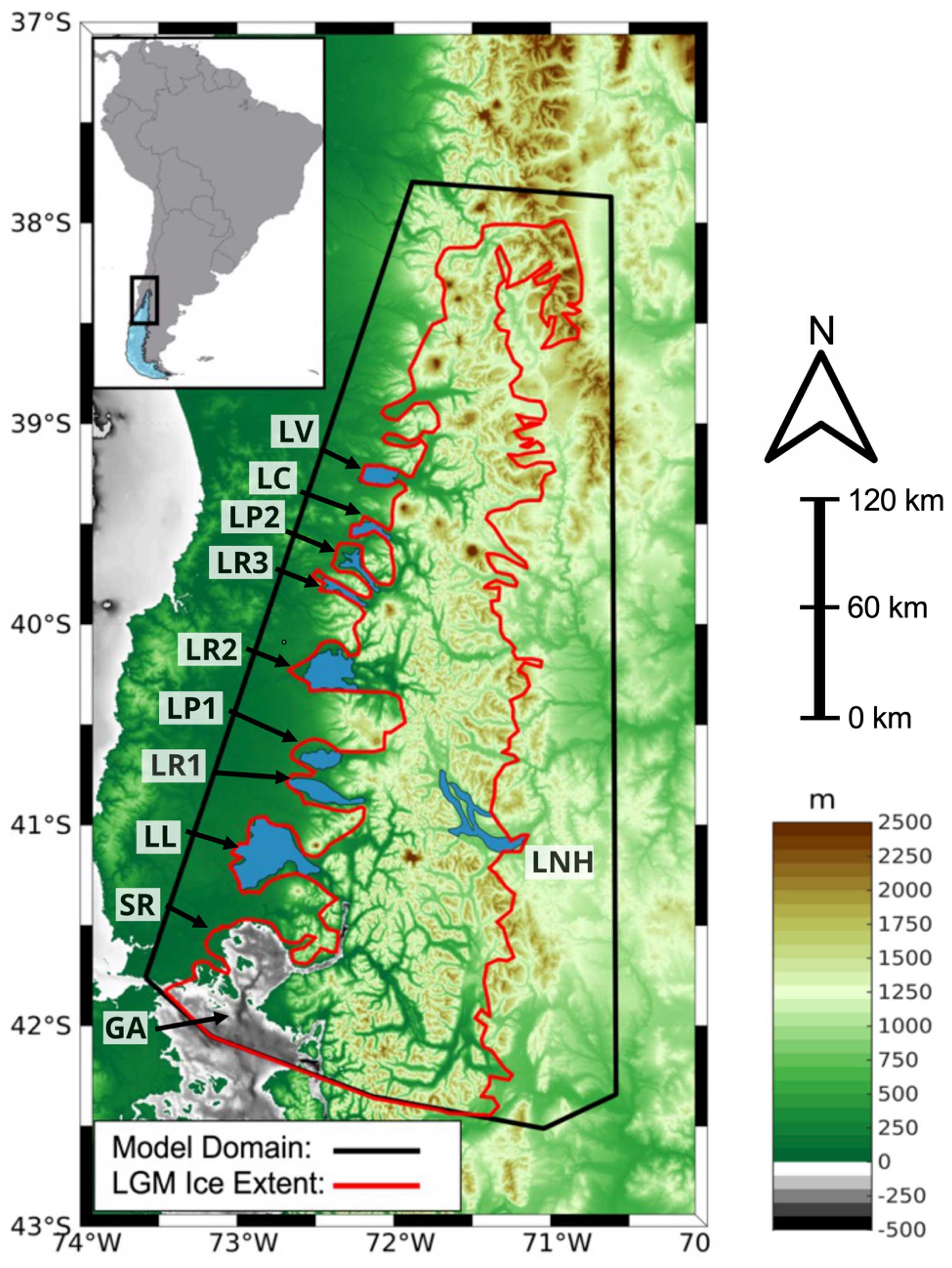
Figure 2 Bedrock topography for our study area (in meters). Our model domain (shown by the black line), encompasses the reconstructed LGM ice limit (shown in red) from PATICE (Davies et al., 2020). Present-day lakes are shown in blue and are abbreviated as follows: SR (Seno de Reloncaví), GA (Golfo de Ancud), LL (Lago Llanquihue), LR1 (Lago Rupanco), LP1 (Lago Puyehue), LR2 (Lago Ranco), LR3 (Lago Riñihue), LP2 (Lago Panguipulli), LC (Lago Calafquén), LV (Lago Villarica), and LNH (Lago Nahuel Huapi).

Although geomorphological evidence suggests that while the southernmost glaciers across the PIS may have been temperate with warm-based conditions during the LGM, there may have been periods when ice lobes were polythermal (Darvill et al., 2017). However, recent ice-flow modeling (Leger et al., 2021b) suggests that varying the ice viscosity mainly impacts the accumulation zone thickness in simulations of paleoglaciers in northeastern Patagonia, with minimal impacts on overall glacier length and extent. Accordingly, based on sensitivity tests (see Supplement Sect. S1), our model is two-dimensional and we do not solve for ice temperature and viscosity, allowing for increased computational efficiency. For our purposes, we use Glen's flow law (Glen, 1955) and set the ice viscosity based on the rate factors in Cuffey and Paterson (2010) assuming an ice temperature of −0.2 °C. We use a linear friction law (Budd et al., 1979):

$$\begin{array}{}\text{(1)}& {\mathit{\tau }}_{\mathrm{b}}=-k^{\mathrm{2}}N{u}_{\mathrm{b}},\end{array}$$

where τ_b represents the basal stress, N represents the effective pressure, and u_b is the magnitude of the basal velocity. Here, $N=g({\mathit{\rho }}_{\mathrm{i}}H+{\mathit{\rho }}_{\mathrm{w}}{Z}_{\mathrm{b}})$, where g is gravity, H is the ice thickness, ρ_I is the density of ice, ρ_w is the density of water, and Z_b is the bedrock elevation following Cuffey and Paterson (2010).

The spatially varying friction coefficient, k, is constructed following Åkesson et al. (2018):

$$\begin{array}{}\text{(2)}& k=\mathrm{200}\times {\displaystyle \frac{min\left[max\left(\mathrm{0},z_{\mathrm{b}}+\mathrm{600}\right),z_{\mathrm{b}}\right]}{max\left(z_{\mathrm{b}}\right)}},\end{array}$$

where z_b is the height of the bedrock with respect to sea level. Using this parameterization, basal friction is larger across high topographic relief and lower across valleys and areas below sea level.

To account for the influence of glacial isostatic adjustment (GIA), we prescribe a transiently evolving reconstruction of relative sea level from the global GIA model of the last glacial cycle from Caron et al. (2018). This includes three physical components: (1) bedrock vertical motion, (2) the eustatic sea level, and (3) geoid changes. The time series we use to prescribe GIA is from the model average of an ensemble of GIA forward model estimations from Caron et al. (2018). The prescribed GIA is in good agreement (Fig. S2 in the Supplement) with a reconstruction of relative sea-level change from an isolation basin in central Patagonia (Troch et al., 2022). This methodology has been applied in recent modeling following Cuzzone et al. (2019) and Briner et al. (2020).

2.2 Experimental design

In order to simulate the ice history at the LGM and across the last deglaciation, we use climate model output from the National Center for Atmospheric Research Community Climate System Model (CCSM3) TraCE-21ka transient climate simulation of the last deglaciation (Liu et al., 2009; He et al., 2013). Monthly mean outputs of temperature and precipitation from these simulations are used as inputs to our glaciological model (full climate forcing details are further described in Sect. 2.4), and we use the monthly mean output every 50 years across the last deglaciation. Large, multi-proxy reconstructions from He and Clark (2022), Liu et al. (2009), He et al. (2013), and Shakun et al. (2012, 2015) have all demonstrated good agreement between TraCE-21ka and a wide variety of paleo-proxy data during the last deglaciation, including records from the West Antarctic and South America.

2.3 Surface mass balance

In order to simulate the deglaciation of the PIS across our model domain, we require inputs of temperature and precipitation to estimate the surface mass balance. To derive the snow and ice melt, we use a positive degree day model (Tarasov and Peltier, 1999; Le Morzadec et al., 2015; Cuzzone et al., 2019; Briner et al., 2020). Our degree day factors for snow melt and bare ice melt are 3 and 6 mm °C⁻¹ d⁻¹, respectively, and we use a lapse rate of 6 °C km⁻¹ to adjust the temperature of the climate forcings to surface elevation; these are within the range of typical values used to model contemporary and paleoglaciers across Patagonia (see Fernandez and Mark, 2016; Table 3; Yan et al., 2022). The hourly temperatures are assumed to have a normal distribution with a standard deviation of 3.5 °C around the monthly mean. An elevation-dependent desertification is included (Budd et al., 1979) which reduces precipitation by a factor of 2 for every kilometer change in ice sheet surface elevation. We note that the values of the surface mass balance parameters were chosen to provide a reasonable fit (to within 5 %) between the simulated LGM ice sheet area and the reconstructed ice area from PATICE (see Figs. 4 and 10).

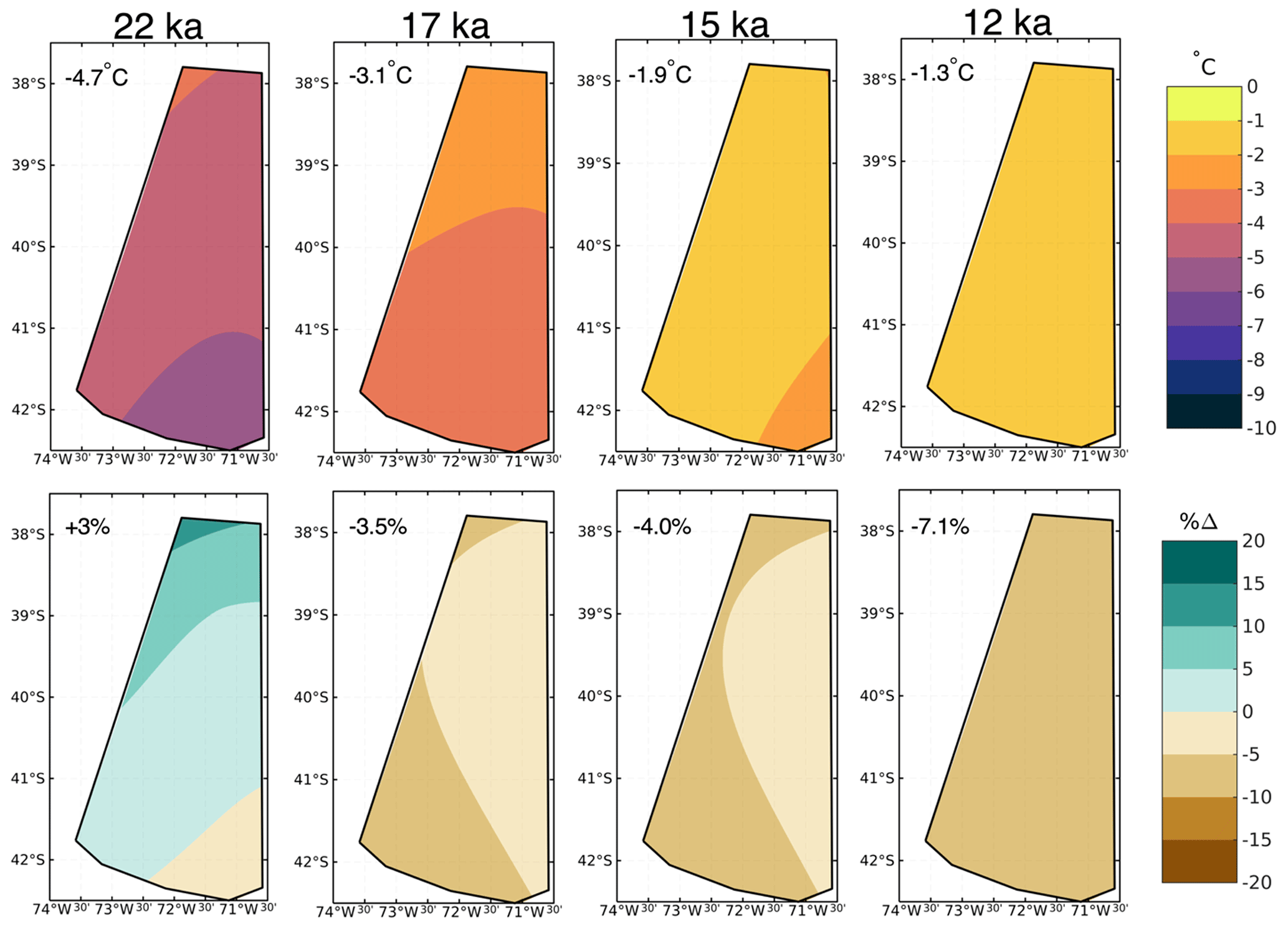
Figure 3 The bilinearly summer (December, January, February (DJF)) temperature (a) and winter (June, July, August (JJA)) precipitation anomalies (b) from TraCE-21ka at 22, 17, 16, and 12 ka. Anomalies are taken as the difference between the LGM and the preindustrial (LGM − PI), with the precipitation anomalies expressed as the percent difference from the preindustrial. The area-averaged value of the anomaly is shown in the upper left corner of each panel.

2.4 Climate forcings

In order to scale monthly temperature and precipitation across the LGM and last deglaciation, we apply a commonly used modeling approach (Pollard and DeConto, 2012; Seguinot et al., 2016; Golledge et al., 2017; Tigchlaar et al., 2019; Clark et al., 2020; Briner et al., 2020; Cuzzone et al., 2022; Yan et al., 2022; Eqs. 3 and 4). First, we use the monthly mean climatology of temperature and precipitation for the period 1979–2018 (${\stackrel{\mathrm{‾}}{T}}_{\text{(1979–2018)}}{\stackrel{\mathrm{‾}}{P}}_{\text{(1979–2018)}})$ from the Center for Climate Resilience Research Meteorological dataset version 2.0 (CR2MET; Boisier et al., 2018). This output, which uses information from a climate reanalysis and is calibrated against rain-gauge observations, is provided at 5 km spatial resolution.

We then bilinearly interpolate these fields onto our model mesh.

$$\begin{array}{}\text{(3)}& {\displaystyle }{T}_t={\stackrel{\mathrm{‾}}{T}}_{\text{(1979–2018)}}+\mathrm{\Delta }{T}_t\text{(4)}& {\displaystyle }{P}_t={\stackrel{\mathrm{‾}}{P}}_{\text{(1979–2018)}}+\mathrm{\Delta }{P}_t\end{array}$$

Next, anomalies of the monthly temperature and precipitation fields from TraCE-21ka (Liu et al., 2009; He et al., 2013) are computed as the difference from the preindustrial control run and interpolated onto our model mesh (ΔT_t and ΔP_t). These anomalies are added to the contemporary monthly mean as shown in Eqs. (3) and (4) to produce the monthly temperature and precipitation fields at LGM and across the last deglaciation (T_t and P_t). In Fig. 3, anomalies of the summer temperature and winter precipitation with respect to preindustrial are shown for 22, 17, 15, and 12 ka.

2.5 Ice front migration and iceberg calving

We simulate calving where the PIS interacts with the ocean, but do not include any treatment of calving in proglacial lakes (see Sect. 4.3). We track the motion of the ice front using the level-set method described in Bondzio et al. (2016; Eq. 3), in which the ice velocity v_f is a function of the ice velocity vector at the ice front (v), the calving rate (c), and the melting rate at the calving front ($\dot{M}$) and where n is the unit normal vector pointing horizontally outward from the calving front. For these simulations the melting rate is assumed to be negligible compared to the calving rate, so $\dot{M}$ is set to 0.

$$\begin{array}{}\text{(5)}& v_{\mathrm{f}}=v-(c+\dot{M})n\end{array}$$

To simulate calving, we employ the more physically based von Mises stress calving approach (Morlighem et al., 2016), which relates the calving rate (c) to the tensile stresses simulated within the ice. In this approach, $\stackrel{\mathrm{̃}}{\mathit{\sigma }}$ is the von Mises tensile strength, ∥v∥ is the magnitude of the horizontal ice velocity, and σ_max is the maximum stress threshold, which has separate values for tidewater and floating ice, namely 1 MPa and 200 kPa, respectively.

$$\begin{array}{}\text{(6)}& c=∥v∥{\displaystyle \frac{\stackrel{\mathrm{̃}}{\mathit{\sigma }}}{{\mathit{\sigma }}_{\max }}}\end{array}$$

The ice front will retreat if the von Mises tensile strength exceeds the user-defined stress threshold. This calving law has been applied in Greenland to assess marine-terminating ice front stability (Bondzio et al., 2016; Morlighem et al., 2016; Choi et al., 2021; Cuzzone et al., 2022), and is applied where ocean is present in our simulations, such as at the Seno de Reloncaví and the Golfo de Ancud (see Fig. 2).

3 Results

3.1 Simulated LGM state

In order to arrive at a steady-state LGM ice geometry, we first initialize our model with an ice-free configuration. A constant LGM monthly climatology of temperature and precipitation is then applied, as is the prescribed GIA from Caron et al. (2018). We allow the ice sheet to relax for 10 000 years, during which the ice sheet is free to grow and expand until it reaches a steady-state ice geometry and volume in equilibrium with the climate forcings.

At 22 ka, TraCE-21ka simulates an area-averaged summertime (DJF) cooling of 4.7 °C relative to the preindustrial PI across our model domain (Fig. 3). The LGM cooling increases from north to south, with the greatest magnitude of cooling, up to 6 °C, occurring across the southern portion of our model domain. During winter (JJA), TraCE-21ka simulates an overall wetter climate across our model domain during the LGM relative to the PI. While the area-averaged LGM precipitation anomaly is small (3 % higher), the LGM precipitation anomaly increases from south to north, with TraCE-21ka simulating 10 %–15 % more wintertime precipitation during the LGM than the PI across the northern portion of the model domain.

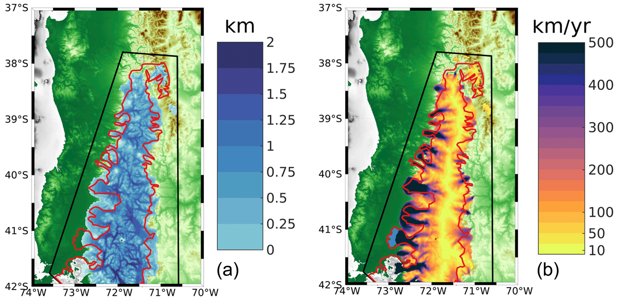
Figure 4 The simulated LGM ice thickness (km; a) and the simulated LGM ice surface velocity (km yr⁻¹; b). The black outline denotes our ice sheet model boundary, and the red line denotes the reconstructed ice extent during the LGM from PATICE (Davies et al., 2020).

Bedrock elevation increases from west to east, with deep valleys interspersed across most of our model domain (Fig. 2). LGM ice thickness is greatest in these valleys (upwards of 2000 m deep), where driving stresses dominate and where the bedrock geometry controls the flow of ice from higher terrain and through these valleys (Fig. 4). Across the highest terrain, such as the many volcanoes across the CLD, the ice is thinner than in the surrounding valleys. An ice divide is present, as slow ice velocities in the interior of the ice sheet give way to fast-flowing outlet glaciers, especially on the western margin of the CLD, where velocities reach in excess of 500 m yr⁻¹ and even up to 2 km yr⁻¹ in some locations. The simulated LGM ice sheet area across the CLD is 414 120 km², which is within 1 % of the area calculated from the PATICE reconstruction (414 690 km²; Fig. 10). This agreement is in part due to the tuning of our degree day factors, as discussed in Sect. 2.3, and gives us confidence in our ability to simulate a reasonable LGM ice sheet across the CLD and throughout the last deglaciation.

3.2 Simulation of the last deglaciation

The monthly mean temperature and precipitation taken every 50 years from the TraCE-21ka (Liu et al., 2009; He et al., 2013) experiment are used to drive our simulation of the ice history across the last deglaciation (22–10 ka). The transient simulation is initialized with the LGM ice sheet geometry shown in Fig. 4 and is run forward with the appropriate climate boundary conditions until 10 ka.

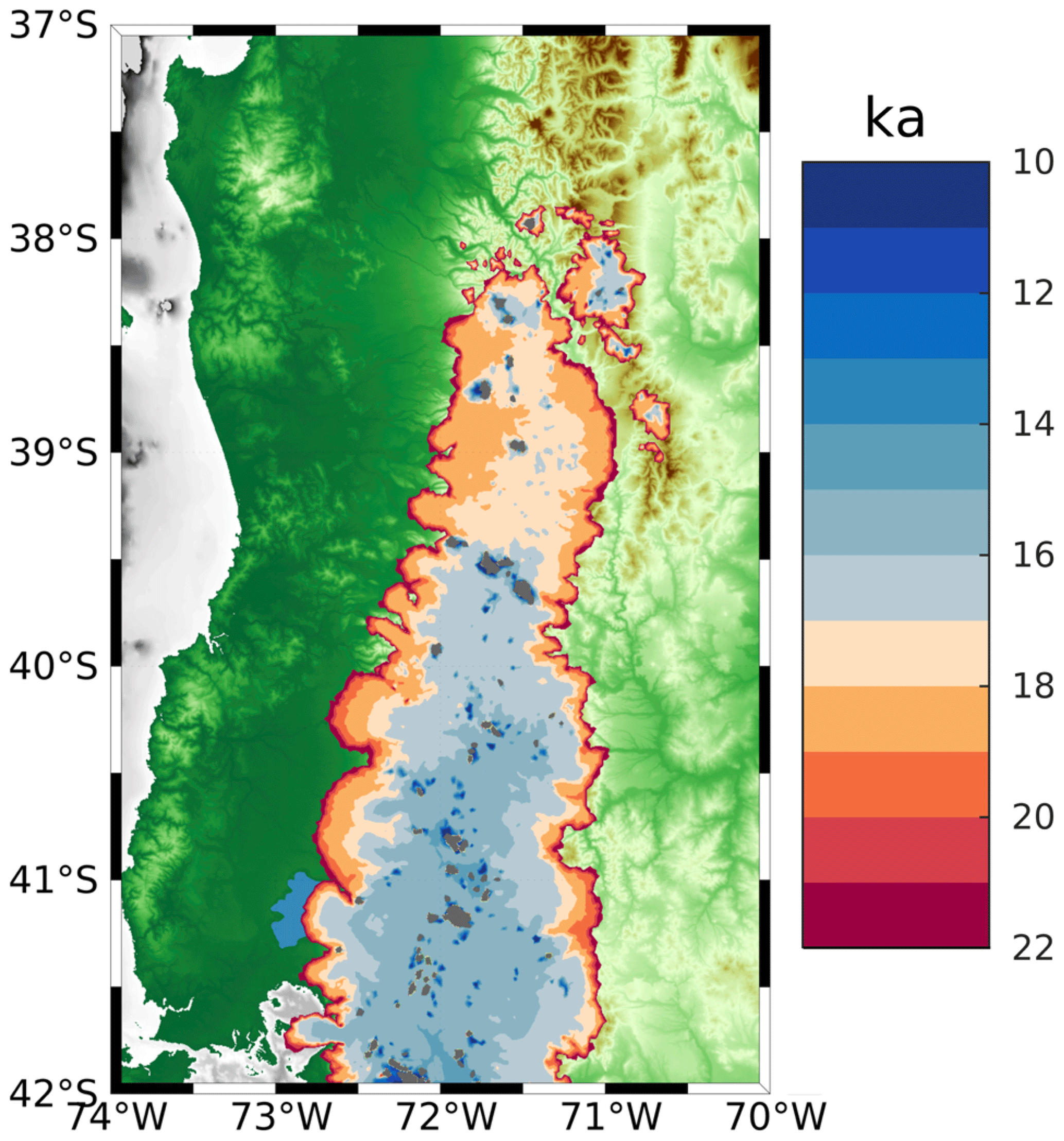
Figure 5 The simulated deglaciation age for the transient simulation from the LGM to 10 ka. The gray color indicates where ice persists after 10 ka.

3.2.1 Pattern of deglaciation

From the resulting transient simulation, we calculate the timing of deglaciation across our model domain (Fig. 5) as the youngest age at which grid points become ice free. Our map of the simulated deglaciation can be paired with a time series of the rate of ice mass change (Fig. 6) to highlight some key features of the magnitude and timing of ice retreat between 22 and 10 ka.

Between 22 and 19 ka, the ice sheet undergoes periods of minor to moderate ice mass loss and gain in an interval of time where summer temperature anomalies (Fig. 6) and the corresponding ice margin remain relatively stable (Fig. 5). Between 19 and 18.5 ka, coincident with a rise in summertime temperature (Fig. 6), a pulse of ice mass loss exceeding 5000 Gt century⁻¹ occurs; after that, the ice loss trends toward minimal ice mass loss at around 18 ka as the rise in summer temperature levels off. During this time interval, the ice margin pulls back considerably towards higher terrain across the northern portion of the model domain (Fig. 5), and many of the fast-flowing outlet glaciers on the western margin retreat back towards the ice sheet interior. Between 18 to 16.2 ka, the summer temperature rises steadily ∼1.2 °C and is punctuated with an abrupt warming of ∼0.5 °C at 16 ka (Fig. 6). During this interval, ice mass loss remains high and steady at ∼1000 Gt century⁻¹, with pulses of increased mass loss varying between 2000–5000⁻¹ occurring at 17.8, 16.8, and 16 ka (Fig. 6).

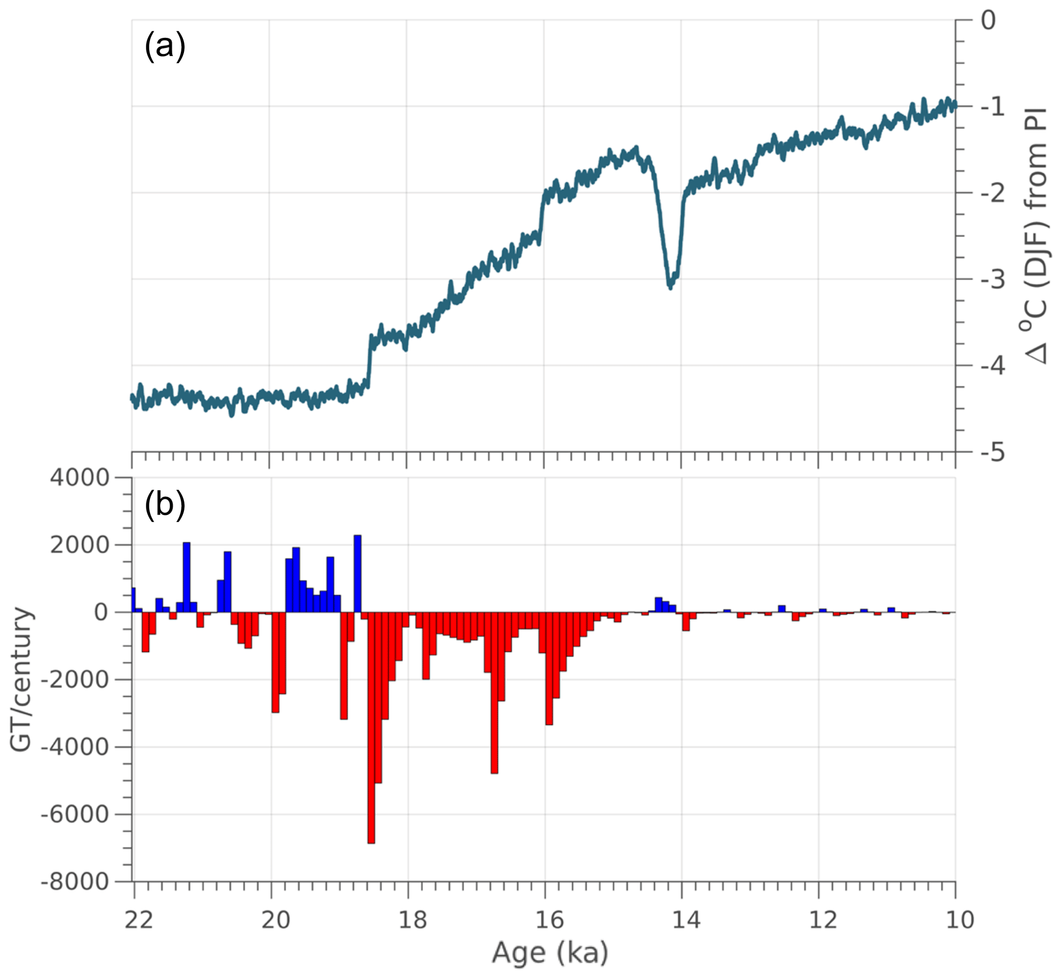
Figure 6 (a) The TraCE-21ka summer (DJF) temperature anomaly, taken as the difference from the preindustrial area averaged across our model domain. (b) The simulated ice mass change, calculated in Gt century⁻¹, across the last deglaciation (22 to 10 ka). Red indicates ice mass loss and blue indicates ice mass gain.

By 17 ka, the northern portion of the model domain (north of 39.5° S) has generally become ice free, with the exception of the highest terrain (e.g., mountain glaciers). By 16 ka, between 39.5 and 40.5° S, ice remains only on the highest terrain (Fig. 5); however, ice cover persists south of 40.5° S. Between 16 and 15 ka, the summer temperature rises by ∼0.5 °C (Fig. 6) and the remaining ice sheet retreats south of 40.5° S. By 15 ka, there is no evidence of an ice sheet, with only mountain glaciers and small ice caps (e.g., Cerro Tronador) existing across the high terrain throughout the model domain (Fig. 5).

After 15 ka, TraCE-21ka simulates a short and abrupt Antarctic Cold Reversal (ACR) between 14.6 and 14 ka (Fig. 6) before temperatures continue to rise into the early Holocene. There is only a minor ice mass gain (e.g., <500 Gt yr⁻¹) during the ACR and minimal fluctuation in ice mass after 14 ka. By 10 ka, only small mountain glaciers persist across the high terrain and volcanoes of the CLD (gray color in Fig. 5).

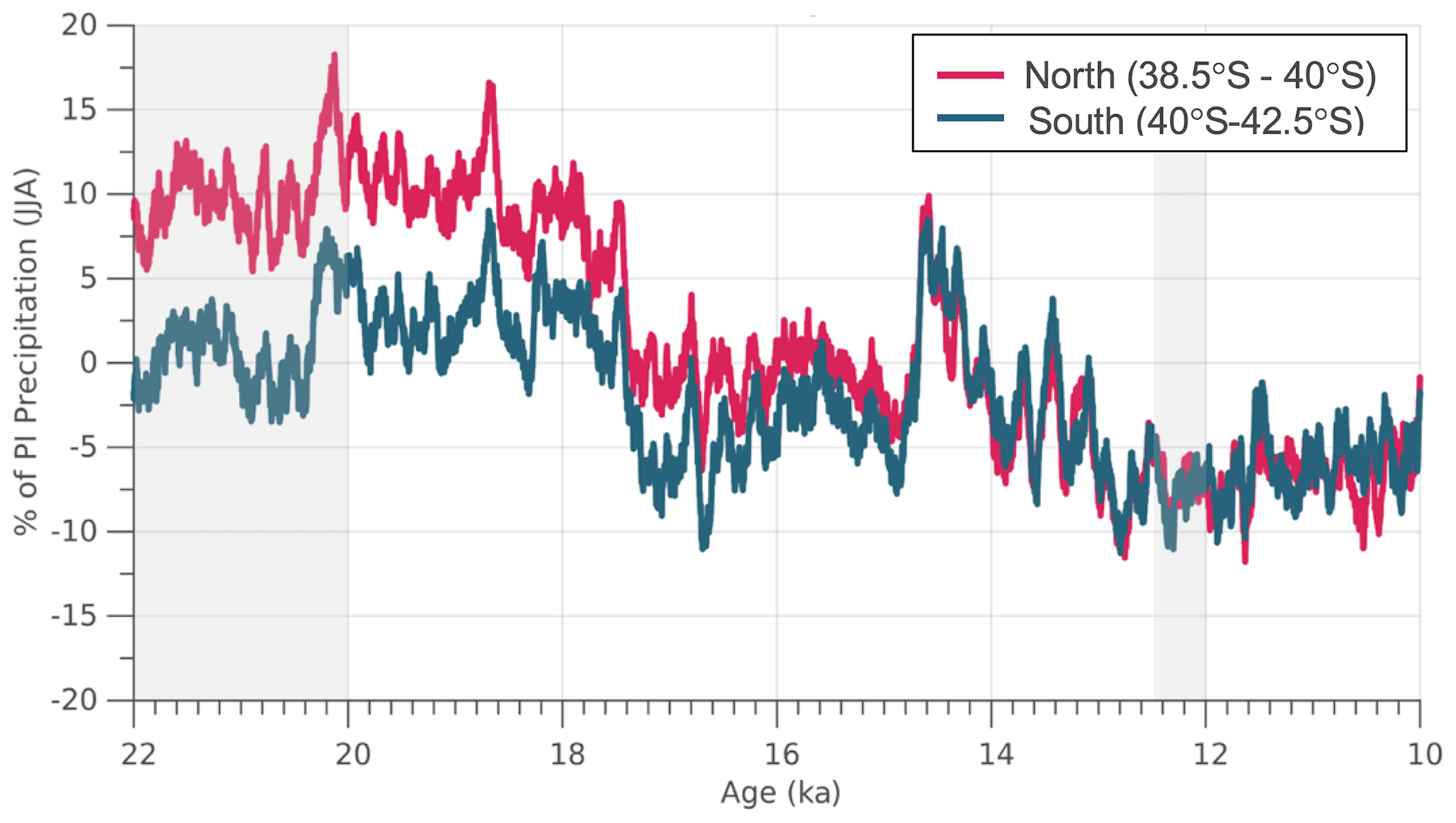
Figure 7 The winter (JJA) precipitation anomaly expressed as the percent difference from the preindustrial period. The area-averaged anomaly is shown for the region north of 40° S and for the region south of 40° S (see Fig. 2 for reference to the latitudinal range of our model domain). The intervals of time used in the sensitivity tests are highlighted by the gray shading.

3.2.2 Sensitivity tests

To better assess how changes in precipitation may modulate the deglaciation across the CLD, we perform additional sensitivity tests. We refer to the simulation discussed above as our main simulation, where the climate boundary conditions of temperature and precipitation vary temporally and spatially across the last deglaciation. Three more simulations are performed where temperature is allowed to vary across the last deglaciation but precipitation remains fixed at a given magnitude for a particular time interval. Each experiment is listed below:

• Precip. PI. Monthly precipitation is held constant at the preindustrial mean. Preindustrial precipitation is reduced compared to the period 22 to 18 ka, but it is similar to and higher than what is simulated after 18 ka, with the exception of the ACR at 14.5 ka (Fig. 7).

• Precip. 12 ka. Monthly precipitation is held constant at the 12.5–12 ka mean. This is a period of reduced precipitation relative to the preindustrial (∼7 % reduction; Fig. 7).

• Precip LGM. Monthly precipitation is held constant at the 22–20 ka mean, which is approximately 10 % higher than preindustrial values across the northern portion of the model domain (north of 40° S).

Across our model domain during the experiment Precip. PI (Fig. 8a), wintertime precipitation during the preindustrial is reduced compared to the early deglaciation (22 to 18 ka) and is similar to or slightly higher than the wintertime precipitation after 18 ka, particularly south of 40° S (Fig. 7). When precipitation is held constant at the preindustrial mean through the last deglaciation, the ice retreats faster across most portions of the model domain, particularly along the ice margins and in the area north of 40° S. In the southern portion of our model domain (south of 40° S), where the changes in deglacial precipitation relative to the preindustrial period are lower (Figs. 3 and 7), the difference in simulated deglaciation age are also smaller. In general, the pace of deglaciation increases by up to 1 kyr compared to the main simulation, with many locations experiencing deglaciation 200–600 years earlier than the main simulation.

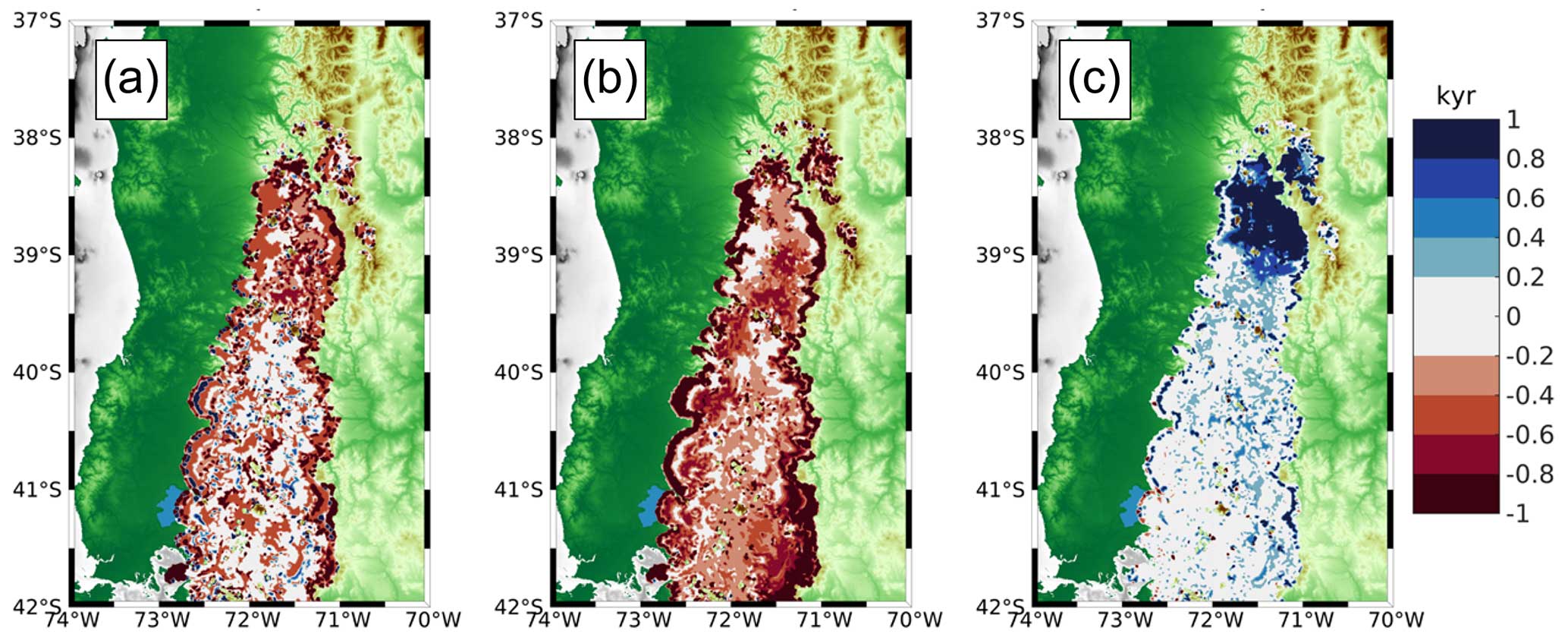
Figure 8 Difference in simulated deglaciation age between sensitivity experiment (a) Precip. PI, (b) Precip. 12 ka, or (c) Precip LGM and the main simulation. Blue colors indicate slower ice retreat for the sensitivity experiments compared to the main simulation, while red colors indicate faster ice retreat for the sensitivity experiments compared to the main run.

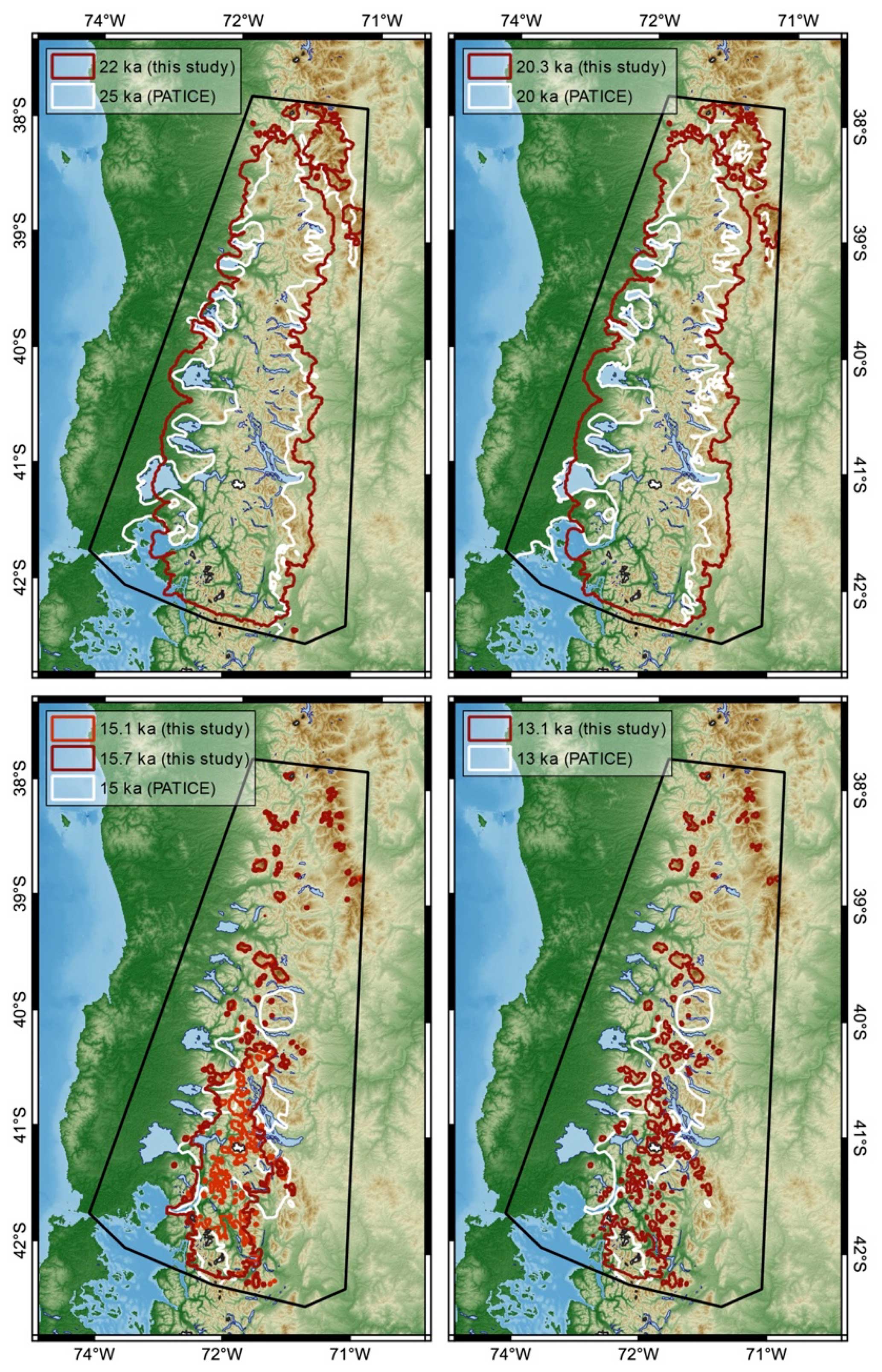
Figure 9 Comparison between the simulated ice extent at time intervals closest to the corresponding reconstructed ice extent from PATICE (Davies et al., 2020).

For the experiment Precip. 12 ka, winter precipitation is reduced by up to 7 % (Fig. 8b) relative to the preindustrial across the model domain (Figs. 3 and 7). In this experiment, the ice retreats faster across most of the CLD from the ice margins and through the interior. Deglaciation along the margins occurs >1 kyr faster in many locations and between 200 years and 1 kyr faster across portions of the ice interior. For the experiment Precip LGM, winter precipitation is increased by up to 10 % (Fig. 8c) across the northern portion of the model domain (north of 40° S) relative to the preindustrial, but it is similar to preindustrial values across the southern portion of our model domain (south of 40° S). In this experiment, with the higher precipitation imposed across the northern portion of the model domain, ice retreats slower during the last deglaciation relative to our standard simulation by >1 kyr, and it does so in some locations by up to 2 kyr.

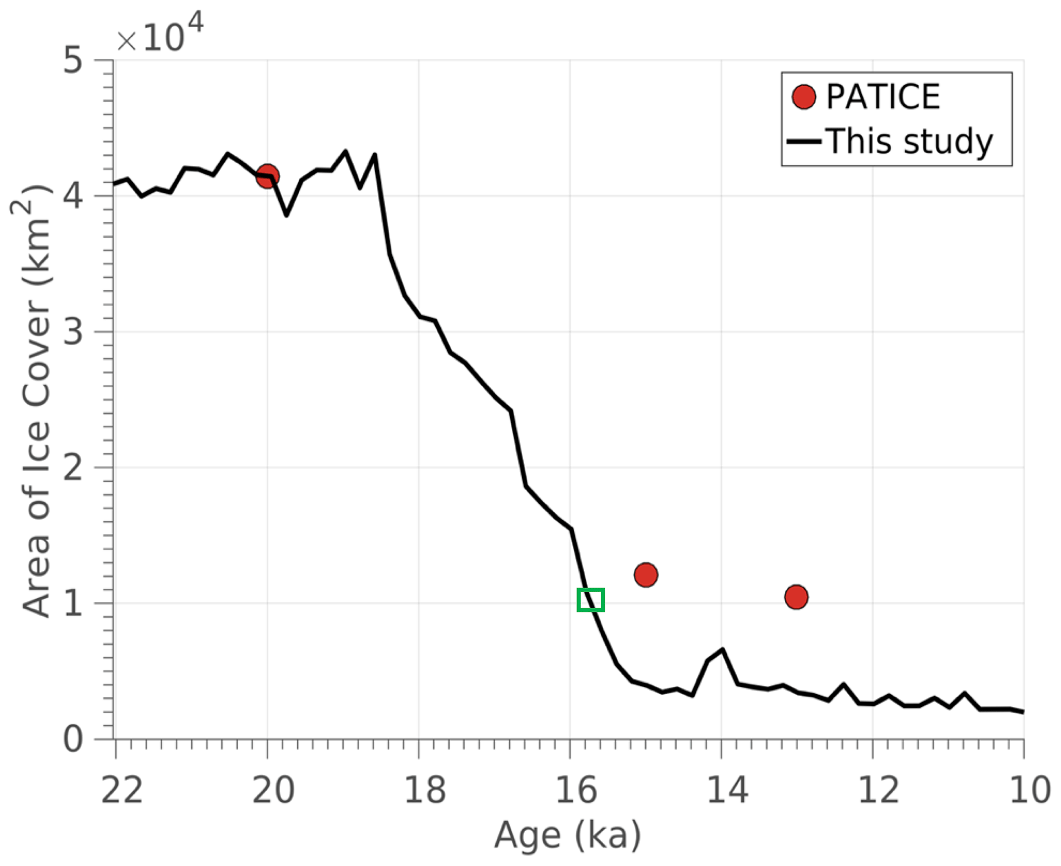
Figure 10 The black line shows the simulated ice area (km²) from 22 to 10 ka. The red dots indicate the calculated ice area across our model domain for the reconstructed ice extent from PATICE (Davies et al., 2020). The green rectangle highlights the simulated ice area at 15.7 ka.

3.3 Comparison to the reconstructed deglacial ice extent

As shown in Fig. 1, PATICE assigns high to medium confidence to the reconstructed LGM (25–20 ka) ice extent along most of the western ice margin and portions of the eastern margin, with low confidence assigned to the northernmost ice extent. The majority of the ice history is poorly constrained (low confidence) during the deglaciation, and PATICE reconstructs a small cap that persists across the southern CLD until 10 ka, after which the ice disappears and only the Cerro Tronador glacier remains (see Fig. 13 from Davies et al., 2020). We show the simulated and reconstructed ice extent in Fig. 9 as well as the calculated ice area from PATICE at 20, 15, 13, and 10 ka and for our transient simulation in Fig. 10. At 22 ka (Fig. 9), our model simulates a generally greater ice extent along the eastern and western margins except at the Senode Reloncaví, Golfo de Ancud, and Lago Llanquihue, where the simulated ice margin does not advance to the well-dated terminal LGM moraines (Mercer, 1972; Porter, 1981; Andersen et al., 1999; Denton et al., 1999). At 20 ka, the simulated ice area is 4.1×10⁴ km², which is nearly identical to the PATICE areal extent across our model domain (Fig. 10). The ice margin at the Seno de Reloncaví, Lago Llanquihue, and other locations along the eastern boundary in the CLD advances slightly at 20 ka but still remains within the PATICE reconstruction for these regions.

Between 18.3 and 15 ka, a large-scale ice retreat occurs, and the simulated ice sheet loses 90 % of its ice area, while the PATICE reconstruction suggests a reduction of 75 % (Fig. 10). At 15 ka, PATICE reconstructs an existing ice cap that separates from the remainder of the PIS to the south (Fig. 9). This is in contrast to the simulated ice extent, which shows that by 15 ka, the PIS across our model domain has completely retreated and only mountain glaciers or small ice caps exist amongst the high terrain. However, if we compare the PATICE area at 15 ka and the simulated ice area at 15.7 ka (Fig. 10; green rectangle), they are nearly identical, 1.2×10⁴ km². While the PATICE ice extent at 15 ka and the simulated ice extent at 15.7 ka do not match completely, the simulated ice extent at 15.7 ka still has evidence of a large ice cap similar to the PATICE reconstruction. Therefore, the simulated transition from ice sheet to ice cap and to discrete mountain glaciers occurs between 15.7 and 15 ka in our simulations. By 13 ka, our simulated ice area is 60 % lower than the PATICE reconstructed area. By 10 ka, this difference is 50 %; however, by this time, the majority of the ice sheet has deglaciated (Fig. 10), with our model simulating discrete mountain glaciers while PATICE reconstructs a small and narrow ice cap across the high terrain in the southern CLD (also see Fig. 1).

4 Discussion

4.1 Climate–ice sensitivity

Determining the influence of the SWW on the heat and hydrologic budgets across South America during the LGM and last deglaciation remains difficult, as paleo-proxy data are limited and climate models tend to disagree on the evolution of the SWW (Kohfeld et al., 2013; Berman et al., 2018). And, while paleo-proxy evidence does suggest wetter conditions across the CLD during the late glacial (Moreno et al., 2018), linking this variability to changes in the position and strength of the SWW remains difficult (Kohfeld et al., 2013).

The scale at which we deduce ice history and climate interactions is also important. Looking at the PIS as a whole, recent numerical ice sheet modeling studies indicate that the simulated ice extent and volume for the entire PIS at the LGM are largely controlled by the magnitude of the temperature anomaly compared to the present day (Yan et al., 2022). However, regional scale ice flow modeling informed by geologic constraints on past ice margin extent show that higher precipitation during the LGM (Leger et al., 2021b), the late glacial, and the Holocene (Muir et al., 2023; Martin et al., 2022) is needed to support model–data agreement. It appears that during the LGM, a northward shift in the SWW (Kohfeld et al., 2013; Rojas et al., 2009; Togweillier et al., 2006) or a strengthening or expansion of the wind belt (Lamy et al., 2010) is perhaps the most likely scenario, with high-frequency variability possible during the deglaciation, as atmospheric reorganization altered the heat and hydrologic budgets as recorded by glacier and ice-sheet change (Davies et al., 2020; Boex et al., 2013).

We analyzed outputs of the wintertime (JJA) 925 hPa zonal wind as the mean over 500-year periods from TraCE-21ka for the LGM (22–21 ka), 18 ka (18.5–18 ka), 16 ka (16.5–16 ka), 14 ka (14.5–14 ka), 12 ka (12.5–12 ka), and the preindustrial period (Sect. S3, Fig. S3a–e). Across our model domain and to its south, relative to the PI, zonal winds are stronger during the LGM, with a southerly displacement (first and second columns in Fig. S3a). At 18 ka (Fig. S3b), the zonal wind increases in strength relative to the PI, with the stronger winds having wider latitudinal coverage, particularly across our model domain. While the mean position of the SWW is poleward at 18 ka relative to the PI (Jiang and Yan, 2022), across Patagonia, the simulated position of the maximum zonal wind is at the same latitudinal band as the PI. At 16 ka, the zonal wind is stronger across our domain and Patagonia (Fig. S3c) relative to the PI, although not as large as the differences at 18 ka. By 14 ka, the strength of the zonal winds across Patagonia and our model domain are similar to or slightly stronger than those in the PI (Fig. S3d); however, the zonal wind maximum is situated more equatorward across our model domain relative to the PI. By 12 ka (Fig. S3e), the zonal wind is similar to or slightly weaker than that in the PI across our model domain, although it is stronger relative to the PI to the south of our model domain across central and southern Patagonia. The position of the maximum zonal winds is also displaced further south relative to the PI. These changes in strength and position of the simulated SWW during the last deglaciation are similar to the findings of Jian and Yan (2020), who found that, relative to the PI, TraCE-21ka simulates a more poleward subtropical and subpolar jet over the Southern Hemisphere at the LGM. During the remainder of the LGM and the last deglaciation, the overall position of the SWW migrates northward in TraCE-21ka, with poleward displacements during Heinrich Stadial 1 (HS1), equatorward displacements during the Antarctic Cold Reversal (ACR), and poleward displacements during the Younger Dryas (YD), similar to our analysis.

Additionally, we evaluated the wintertime (JJA) low-level (850 hPa) moisture flux convergence from TraCE-21ka (MFC; Sect. S4, Fig. S4a–e), which is influenced by the mean flow and transient eddies in the extratropical hydrologic cycle (Peixoto and Oort, 1992). During the LGM and at 18 ka, MFC increases across our model domain, consistent with a convergence of the mean flow moisture fields relative to the PI (Fig. S4a, b). During the LGM and at 18 ka, we note that TraCE-21ka simulates higher JJA precipitation anomalies (relative to the PI) across our model domain (Fig. 7). While our analysis cannot directly constrain the source of the positive precipitation anomalies (e.g., mean flow, storms), the strength of the simulated SWW in TraCE-21ka increases across our model domain (Fig. S3a, b) coincident with the increases in MFC, which may contribute to the positive precipitation anomalies at these time intervals (Fig. 7). By 16 ka, there is increased divergence in the 925 hPa winds and moisture relative to the PI (Fig. S4c). Decreased MFC relative to the PI coincides with a reduction in precipitation across our model domain that is similar to or less than the PI (Fig. 7). We note that the ice thickness boundary conditions used in TraCE-21ka come from the Ice5G reconstruction (Peltier, 2004), which has the PIS being completely deglaciated by 16 ka. However, our analysis cannot decompose whether the simulated changes in precipitation and MFC are a consequence of the coupling between regional atmospheric circulation and the ice thickness boundary conditions used in TraCE-21ka or if these changes represent wider interactions with changes in hemispheric atmospheric circulation. By 14 ka, and during the ACR, MFC increases relative to the PI (Fig. S4d). This is consistent with a simulated equatorward migration of the SWW, as shown in Jiang and Yan (2020) and our analysis (Fig. S3d), and positive anomalies in precipitation across our model domain relative to the PI (Fig. 7). By 12 ka, precipitation across our model domain is reduced relative to the PI (Figs. 3 and 7), and TraCE-21ka simulates a reduction in the MFC as well as a poleward migration of the SWW (Fig. S3e; Jiang and Yan, 2020).

When considering proxy records of precipitation across the CLD, there is reasonable agreement with the changes in precipitation simulated by TraCE-21ka. Moreno et al. (1999, 2015) and Moreno et al. (2018) find that wetter than present-day conditions existed across the CLD during the LGM and early deglaciation, which is consistent with the precipitation anomalies simulated by TraCE-21ka (Figs. 3 and 7). These changes in paleoclimate proxies are attributed to an intensified storm track associated with an equatorward shift of the SWW (Moreno et al., 1999, 2015). While TraCE-21ka instead simulates a poleward shift of the SWW during these time intervals, increases in precipitation and the intensification of the storm track as inferred by Moreno et al. (2015) may also be consistent with a strengthening of the SWW as simulated by TraCE-21ka during these intervals (Fig. S3a, b; Rojas et al., 2009; Sime et al., 2013; Kohfeld et al., 2013). Moreno et al. (2015) note that rapid warming ensues across the CLD around 17 800 cal yr BP, which is similar to the timing of deglacial warming as simulated by TraCE-21ka at around 18.5 ka (Fig. 6). Coincident with this rapid temperature rise, Moreno et al. (2015) note a shift from hyperhumid to humid conditions, which aligns well with decreases in the simulated precipitation in TraCE-21ka across our model domain (Fig. 7). Lastly, Moreno et al. (1999, 2015) find that colder and wetter conditions occur across the CLD during the ACR and infer an equatorward expansion of the SWW as a potential cause. While TraCE-21ka simulates an abrupt and short ACR, it does simulate an equatorward expansion of the SWW (Fig. S4d; Jian and Yan, 2020), associated cooling (Fig. 6), and increases in precipitation (Fig. 7) that agree with the proxy data.

Prior numerical ice flow modeling has indicated that precipitation played an important role in controlling the extent of paleoglaciers across the PIS (Muir et al., 2023; Leger et al., 2021b) by modulating the pace and magnitude of ice retreat and advance during deglaciation (Martin et al., 2022). Many of the TraCE-21ka-simulated winter precipitation anomalies shown in Figs. 3 and 7 are within 10 % of the preindustrial value. The sensitivity tests conducted here suggest that modest changes (∼10 %) in precipitation can alter the pace of ice retreat across the CLD on timescales consistent with the resolution of geochronological proxies constraining past ice retreat. We note that while TraCE-21ka simulates variations in precipitation across our model domain that are consistent with hydroclimate proxies discussed above (Moreno et al., 1999, 2015, 2018), the magnitude of those changes is not as large as proxy data across the CLD indicate. For example, hydroclimate proxies suggest that the LGM and early deglaciation were up to 2 times wetter across the CLD than the present day (Moreno et al., 1999). Therefore, we can deduce from our sensitivity analysis here that higher precipitation anomalies during the LGM and last deglaciation, forced by proposed changes in the SWW (Moreno et al., 1999, 2015), may have helped offset melt from deglacial warming, thereby influencing the pacing of early deglacial ice retreat in this region.

4.2 Ice retreat during the last deglaciation

The PATICE dataset (Davies et al., 2020) serves as the best available reconstruction of ice margin change for the PIS across the last deglaciation. This state-of-the-art compilation provides an empirical reconstruction of the configuration of the PIS as isochrones every 5 ka from 35 ka to the present based on detailed geomorphological data and available geochronological evidence. Because geochronological constraints on past PIS change are limited, particularly in the CLD, the PATICE reconstruction assigns qualitative confidence to its reconstructed ice margins. Where there is agreement between geochronological and geomorphological indicators of past ice margin history (i.e., moraines), high confidence is assigned. Where geomorphological evidence suggests the existence of past ice margins but lacks a geochronological constraint, medium confidence is assigned. Lastly, low confidence is assigned where there is a lack of any indicators of past ice sheet extent and where the ice limits result in interpolated interpretations from immediately adjacent moraines from valleys that have been mapped and dated. Across the CLD, the LGM (25, 20 ka) ice extent is well constrained by geologic proxies, particularly in the west and southwest (Fig. 1). The moraines that constrain the piedmont ice lobes that formed along the western boundary have reasonable age control (Denton et al., 1999; Moreno et al., 1999; Lowell et al., 1995), giving us confidence in the LGM ice margin limits. Beyond this region, age control is sparse along the western boundary for the timing of LGM ice extent, but the existence of well-defined moraines along lakes in the northern CLD are assumed to be in sync with those moraines deposited to the south (Denton et al., 1999). However, low confidence remains in the geologic reconstruction of the LGM ice boundary along the eastern margin, where few to no chronological constraints are available. In general, deglaciation from the maximum LGM ice extent begins between 18–19 ka (Davies et al., 2020); however, poor age control and a lack of geomorphic indicators make it difficult to constrain the ice extent across this region during the deglaciation. For instance, a single cosmogenic nuclide surface exposure date retrieved from the Nahuel Huapi moraine yielded an age of ∼31.4 ka (Zech et al., 2017; 41.04° S, 71.15° W). While it is assumed that the ice limit behaved similarly both to the west and to the east, the limited existing data prevent a comprehensive understanding of the ice extent at the northeastern margin. This induces the highest level of uncertainty in the reconstruction and hinders our data model comparison. Therefore, we rely on the PATICE dataset's interpolated isochrones (low confidence) for this northeastern region as the state-of-the-art reconstruction.

In regards to ice area and extent, our simulated ice sheet at the LGM using TraCE-21ka climate boundary conditions agrees well with the PATICE reconstruction (Fig. 10). Our simulations reveal that deglaciation began at between 19 ka and 18 ka, consistent with the reconstruction by Davies et al. (2020). Notably, the simulated timing of deglaciation agrees with moraine records further south on the eastern side, such as those in Río Corcovado (∼43° S, Leger et al., 2021a; 17.9 ka), Río Cisnes (∼44° S, Garcia et al., 2019; ∼19 ka), Lago Palena/General Vintter (∼44° S, Soteres et al., 2022; 19.7 ka), and Río Ñirehuao (∼45° S, Peltier et al., 2023; ∼18.5 ka). On the other hand, glaciers are thought to have withdrawn from their LGM position later (∼18–17 ka) at the northwestern margin (∼41° S, Denton et al., 1999; Moreno et al., 2015) and in the southern (∼46° S, Kaplan et al., 2004) and southernmost (∼52° S, McCulloch et al., 2000, 2005; Kaplan et al., 2008; Peltier et al., 2021) regions. The simulated ice retreat continues until 15 ka, with the largest pulses in ice mass loss occurring at 18.6, 16.8, and 16 ka (Fig. 6). Where PATICE estimates an ice cap at around 15 ka (∼40° S), our simulations reveal that glaciation was restricted to high elevations. After 15 ka, mountain glaciers remain in our simulation, but there is no presence of a large ice cap as reconstructed in PATICE. Comparison between the model simulations and PATICE becomes difficult during the 15–13 ka period, as confidence in the geologic reconstruction is low due to a lack of geochronological and geomorphological constraints on past ice history. Therefore, our model results offer a different reconstruction from PATICE and indicate that the ice sheet in this region had largely retreated by 15 ka, with only mountain glaciers remaining. This is supported further south, where the ice sheet disintegrated at ∼16 ka, with the paleolake draining into the Pacific Ocean (∼43° S, Leger et al., 2021a) and the ice remaining limited to higher mountain areas. However, during this interval, the Antarctic Cold Reversal (ACR) may have influenced the heat and hydrologic budgets across this region, with wetter and cooler conditions interrupting the deglacial warming (Moreno et al., 2018). While TraCE-21ka simulates a cooler and wetter ACR, it is short-lived, lasting about 500 years as compared to 2000 years in some ice core records or proxy-based studies (Lowry et al., 2019; He et al., 2013, Pedro et al., 2016). This potential for a favorable and prolonged period of glacier growth is likely missing in our simulations during the ACR.

4.3 Limitations

Currently, ISSM is undergoing model development to include a full treatment of solid earth–ice and sea-level feedbacks (Adhikari et a., 2016). Therefore, at this time, there is no coupling between the ice sheet and solid earth. Instead, we prescribed GIA from a global GIA model of the last glacial cycle from Caron et al. (2018). While this model reasonably estimates GIA across the PIS over the last deglaciation, our simulated ice history does not feedback into the GIA. The ice history for Patagonia incorporated into the Caron et al. (2018) ensemble is from Ivins et al. (2011). Therefore, the prescribed GIA response across our domain does not perfectly match our simulated ice history. Additionally, the global mantle from Caron et al. (2018) does not exhibit the regional low viscosity that is attributable to Patagonia, and therefore current rates of deformation are likely underestimated by the model. By not simulating the two-way-coupled ice and solid-earth interactions, we could be missing some feedbacks between our simulated ice history and the solid earth that may modulate the deglaciation across this region. Despite this limitation, however, our prescribed GIA from Caron et al. (2018) is reasonable when compared with the reconstructed deglacial GIA in Patagonia (Troch et al., 2022; see Fig. S2), giving us confidence that our simulation is capturing the regional influence of GIA on the simulated ice history.

Across most of our domain, moraines formed from glacio-tectonized outwash (Bentley, 1996) provide evidence for an advance of piedmont glaciers across glacial outwash during the LGM, which formed the physical boundary for some of the existing terminal moraines around the lakes within the CLD (Bentley, 1996, 1997). The formation of ice-contact proglacial lakes likely occurred as a function of deglacial warming as ice retreated into overdeepenings in the bedrock topography and filled with meltwater (Bentley, 1996). Where there were proglacial lakes along the westward ice front in the CLD, evidence suggests that ice was grounded during the LGM (Lago Puyehue; Heirman et al., 2011). During deglaciation, proglacial lakes formed along the ice sheet margin (Bentley, 1996, 1997; Davies et al., 2020), with evidence suggesting that the local topography and calving may have influenced the spatially varying retreat rates along these margins (Bentley, 1997). Recent glacier modeling (Sutherland et al., 2020) suggests that the inclusion of ice–lake interactions may have large impacts on the magnitude and rate of simulated ice front retreat, as ice–lake interactions promote greater ice velocities, ice flux to the grounding line, and surface lowering. However, how much the proglacial lakes in the CLD may have influenced local deglaciation is not well constrained (Heirman et al., 2011). While more geomorphic data are needed, recent work south of our study region (46.5° S) reconstructed early deglacial ice retreat using a glaciolacustrine varve record from Lago General Carrera–Buenos Aires (Bendle et al., 2019). The authors find that, following an initial retreat due to deglacial warming, the ice margin retreated into a deepening proglacial lake, which accelerated ice retreat in this region due to persistent calving, therefore supporting the role proglacial lakes likely played across the margins of the retreating PIS during the last deglaciation. Because the inclusion of ice–lake interactions is relatively novel for numerical ice flow modeling (Sutherland et al., 2020; Quiquet et al., 2021; Hinck et al., 2022), we choose not to simulate the evolution and influence of proglacial lakes on the deglaciation across this model domain. Given this limitation, our simulated magnitude and rate of ice retreat at the onset of deglaciation may be underestimated, especially when looking at local deglaciation along these proglacial lakes. Although we do not think that these processes would greatly influence our conclusions regarding the role of climate in the evolution of the PIS in the CLD and the simulated ice retreat history, future work is required to assess the influence of proglacial lakes in this region.

5 Conclusions

In this study, we used a numerical ice sheet model to simulate the LGM and deglacial ice history across the northernmost extent of the PIS, the CLD. The ice sheet model used inputs of temperature and precipitation from the TraCE-21ka climate model simulation covering the last 22 000 years in order to simulate the deglaciation of the PIS across the CLD into the early Holocene.

Our numerical simulation suggests that large-scale ice retreat occurs after 19 ka, coincident with rapid deglacial warming, with the northern portion of the CLD becoming ice free by 17 ka. The simulated ice retreat agrees well with the most comprehensive geologic assessment of past PIS history available (PATICE; Davies et al., 2020) for the LGM ice extent and early deglacial but diverge when considering the ice geometry at and after 15 ka. In our simulations, the PIS persists until 15 ka across the remainder of the CLD, followed by ice retreat to higher elevations as mountain glaciers and small ice caps persist into the early Holocene (e.g., Cerro Tronador). The geologic reconstruction from PATICE instead estimates a small ice cap persisting across the southern portion of high terrain in the CLD until about 10 ka. However, given the limited geologic constraints, particularly after 15 ka, high uncertainty in the timing and extent of deglaciation remains in the geologic reconstruction. Therefore, our results provide an additional reconstruction of the deglaciation of the PIS across the CLD that differs from PATICE after 15 ka, emphasizing a need for future work that aims to improve geologic reconstructions of past ice margin migration, particularly during the later deglaciation across this region.

While deglacial warming was a primary driver of the demise of the PIS across the last deglaciation, we find that precipitation modulates the pacing and magnitude of deglacial ice retreat across the CLD. Paleoclimate proxies within the CLD have shown that the strength and position of the SWW varied during the LGM and last deglaciation, altering hydrologic patterns and influencing the deglacial mass balance. We find that the simulated changes in the strength and position of the SWW in TraCE-21ka are similar to those inferred from paleoclimate proxies of precipitation, consistent with a wetter than preindustrial climate being simulated and reconstructed over the CLD and in particular the region north of 40° S. Through a series of sensitivity tests, we altered the magnitude of the precipitation anomaly modestly (up to 10 %) during our transient deglacial simulations and found that the pacing of ice retreat can speed up or slow down by between a few hundred years and up to 2000 years depending on the imposed increase or decrease in the precipitation anomaly. While paleoclimate proxies of precipitation suggest that the CLD may have experienced twice as much precipitation during the LGM and early deglacial relative to the present day (Moreno et al., 1999, 2015), TraCE-21ka simulates smaller increases in LGM and early deglacial precipitation (∼10 %–15 % greater than preindustrial). Therefore, while our modeling suggests that modest changes in precipitation can modulate the pace of deglacial ice retreat across the CLD, from our analysis, we can deduce that larger anomalies in precipitation, as found in the paleoclimate proxies, may have an even larger impact on modulating deglacial ice retreat. Because paleoclimate proxies of past precipitation are often lacking and climate models can simulate a range of possible LGM and deglacial hydrologic states, these results suggest that improved knowledge of past precipitation is critical to achieving a better understanding of the drivers of PIS growth and demise, especially as small variations in precipitation can modulate the ice sheet history on scales consistent with geologic proxies.