the Creative Commons Attribution 4.0 License.
the Creative Commons Attribution 4.0 License.
 | 01 Mar 2023
Fusion of Landsat 8 Operational Land Imager and Geostationary Ocean Color Imager for hourly monitoring surface morphology of lake ice with high resolution in Chagan Lake of Northeast China
Qian Yang
Xiaoguang Shi
Weibang Li
Kaishan Song
Zhijun Li
Xiaohua Hao
Fei Xie
Nan Lin
Zhidan Wen
Chong Fang
Ge Liu
The surface morphology of lake ice remarkably changes under the combined influence of thermal and mechanical forces. However, research on the surface morphology of lake ice and its interaction with climate is scarce. A large-scale linear structure has repeatedly appeared on satellite images of Chagan Lake in recent years. The Geostationary Ocean Color Imager (GOCI), with a 1 h revisit, and Landsat 8 Operational Land Imager (OLI), with a spatial resolution of 30 m, provide the possibility for the study of hourly changes in the large-scale linear structure. We merged the Landsat and GOCI images, using an Enhanced Spatial and Temporal Adaptive Reflectance Fusion Model (ESTARFM), and extracted the lengths and angles of the linear structure. We monitored the hourly changes in the surface morphology during the cold season from 2018 to 2019. The average length of the linear structure in the completely frozen period was 21 141.57 ± 68.36 m. The average azimuth angle was 335.48 ± 0.23∘, nearly perpendicular to the domain wind in winter. Through two field investigations during the two recent cold seasons, we verified the linear structure as being ice fractures and ridges. The evolution of surface morphology is closely associated with air temperature, wind, and shoreline geometry.
- Article
(11737 KB) - Full-text XML
- BibTeX
- EndNote


Lake ice is one of the essential climate variables in the cryosphere (Bojinski et al., 2014) and is closely associated with lake environments, ecological regulation, public transportation, and the safety of human activities (Hampton et al., 2017; Magnuson et al., 2000; Leppäranta, 2015; Brown and Duguay, 2010; Arp et al., 2020). The shortening of the ice cover duration and the thinning of ice thickness have been common trends throughout the world (IPCC, 2021; SROCC, 2019; Murfitt and Duguay, 2021). Recent work using remote sensing mainly focused on lake ice phenology (Weber et al., 2016; Zhang et al., 2021; Xie et al., 2020; Murfitt and Duguay, 2020; Du et al., 2017), lake ice classification (Hoekstra et al., 2020), ice thickness (Murfitt et al., 2018b; Kang et al., 2014; Gogineni and Yan, 2015), and ice albedo (Li et al., 2018; Lang et al., 2018). However, previous work on the surface morphology of lake ice is scarce. The surface morphology, i.e., ice ridges and fractures, is controlled by the dynamic processes of lake ice, which have attracted widespread concern in academia and the society. In this study, we monitored the surface morphology of Chagan Lake in Northeast China by combining high spatiotemporal remote sensing data and the results of field investigations and explored the potential influences of climate factors.
Satellite remote sensing is macroscopic, multi-source, and wide-ranging and has been successfully applied in the global remote sensing monitoring of lake ice (Murfitt and Duguay, 2021; Doernhoefer and Oppelt, 2016; Du et al., 2019). Visible light and multispectral data were first used to monitor lake ice based on the spectral difference between ice and water; however, the best period to monitor lake ice changes is prone to be missed due to the influences of clouds, fog, and light (Howell et al., 2009; Cai et al., 2019; Yang et al., 2019; Qi et al., 2020). Active microwave data are used to identify ice through the differences in the backscatter of water and ice, while passive microwave data are used to identify ice through the differences in brightness temperature (Cai et al., 2017). Microwave remote sensing can penetrate the dry snow on the surface of lake ice and observe the internal structure and stratification of lake ice (Jones et al., 2013) from the early stage of the qualitative differentiation between ground ice and floating ice to the quantitative inversion of the phenology and thickness of lake ice (Ke et al., 2013; Jeffries et al., 2013; Howell et al., 2009; Kang et al., 2014). Although the temporal resolution of active microwave remote sensing data has been improved from 30 d (ERS – European Remote Sensing) to daily return visits (Radarsat-2), the optimized technique is too costly and more suitable for case studies of small or medium lakes (Murfitt et al., 2018a; Geldsetzer et al., 2010). With a high temporal resolution and temporal coverage, passive remote sensing data can detect ice cover under all weather conditions and are limited by their low spatial resolution and significant mixed image effects. Thus, passive remote sensing is more suitable for monitoring large-scale lake ice (Du et al., 2017; Qiu et al., 2018). Although multi-source remote sensing is available to monitor lake ice processes, single-sensor remote sensing data cannot simultaneously achieve both accurate remote sensing monitoring and a high frequency.
The growth and decay processes of lake ice change very fast, requiring high temporal resolution to capture surface morphology. Satellite sensors with moderate spatial resolution, such as Visible Infrared Imaging Radiometer (VIIRS) and Moderate Resolution Imaging Spectroradiometer (MODIS), can monitor the temporal changes in lake ice daily but fail to reflect the spatial details of surface morphology. Satellite sensors with medium spatial resolution, such as Landsat and Sentinel, can provide fine-texture images but do not have frequent images to capture fast changes. Fusion methods include the unmixing method, weight function method, and dictionary–pair learning method (Sisheber et al., 2022; Zhu et al., 2016). The most common weight function method includes the Spatial and Temporal Adaptive Reflectance Fusion Model (STARFM; Feng et al., 2006), Spatial and Temporal Adaptive Algorithm (STAARCH; Hilker et al., 2009), Enhanced Spatial And Temporal Adaptive Reflectance Fusion Model (ESTARFM; Zhu et al., 2010), and Flexible Spatiotemporal Data Fusion (FSDAF; Zhu et al., 2016). Previous studies have proven that these spatiotemporal fusion methods can improve the monitoring abilities of remote sensing for specific applications, but that they fail to monitor the abrupt changes in landscapes and spectral differences. All these models are derived by pairs of coarse and fine resolution, e.g., one pair for the STARFM and two pairs for the ESTARFM. The ESTARFM method performs better than the STARFM in heterogeneous landscapes (Zhu et al., 2010; Knauer et al., 2016; Y. Wang et al., 2021; Jarihani et al., 2014). When monitoring spatial changes, the STAARCH method strictly requires two pairs of bases, including one before and one after the changes, which limits its wide application. The FSDAF is more robust than the other three methods but has limitations in detecting tiny changes (Zhu et al., 2016), making it difficult to monitor the changes in surface morphology. Therefore, we generated fusion images with a high spatiotemporal resolution based on the ESTARFM for further exploration.
The evolution of a lake ice season is mainly a thermodynamic process influenced by thermal and mechanical forces. Thermal forces enable the surface to melt and freeze at the turn of the day and night, and the mechanical strength of winds and currents makes the ice bulk move and collide, causing water courses, ice ridges, and ice fractures to appear, develop, and disappear. Therefore, the surface morphology of lake ice exhibits a periodical spatiotemporal difference, which differs significantly from the flat and smooth surface of lake ice. The horizontal and linear structures of lake ice are monitored by optical satellites for large lakes in Europe and have been explained by ice displacement (Leppäranta, 2015). High-resolution satellite–airborne synthetic-aperture radar (SAR) images have been used to monitor the surface deformation of sea ice, such as ice ridges (Dierking, 2010). Moreover, airborne aerial platforms, such as unmanned aerial vehicles (UAVs; Li et al., 2020), airborne radar (Jeffries et al., 2013), and ground-penetrating radar (Gusmeroli and Grosse, 2012), have effectively complemented remote sensing data sources to monitor the changes in the morphology of lake ice. The spatial distribution of the surface morphology of lake ice is complex, variable, and discontinuous, which is characterized by highlighting linear features on remote sensing images. Currently, there are few studies on the changes in the surface morphology of lake ice and the influence factors. It is meaningful to develop a quantitative method to describe the surface morphology and explore the potential influences.
This study proved the capability of high spatiotemporal remote sensing images for monitoring the surface morphology of lake ice in Chagan Lake, Northeast China. Our work aimed to (1) generate high spatiotemporal satellite images using Landsat and the Geostationary Ocean Color Imager (GOCI), (2) monitor the hourly spatial changes in the surface morphology, including the length and angle, of Chagan Lake, and (3) discuss the beneficial climate conditions during the formation of the surface morphology of lake ice.
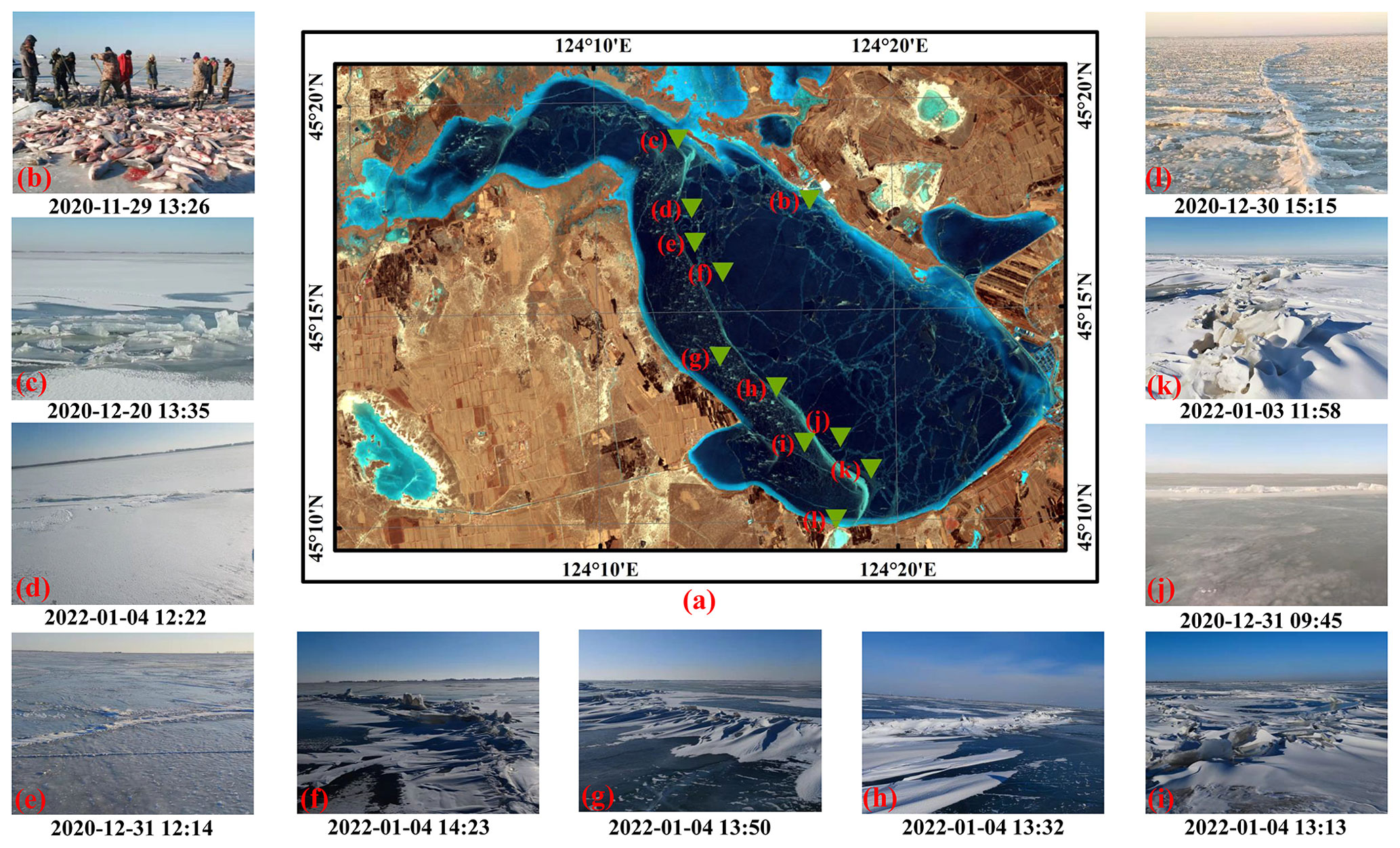
Figure 1The spatial distribution of Chagan Lake and field photographs. Panel (a) is provided by the Landsat 8 Operational Land Imager (OLI) on 10 February 2019, with the band composite of R(5) + G(4) + B(3). Panels (b)–(h) display the field photographs captured in field investigations.
2.1 Study area
As one of the 10 largest lakes in China, Chagan Lake (124∘03′–124∘34′ E, 45∘09′–45∘30′ N; Fig. 1) plays an essential role in fisheries, agricultural irrigation, and winter recreation in the surrounding areas (Wen et al., 2020). The average and maximum water depths are 2.5 and 4.5 m, respectively (Duan et al., 2007; Song et al., 2011). The lake has a water area of 329.72 km2 and a perimeter of 201.03 km, according to the Landsat 8 Operational Land Imager (OLI), on 10 January 2019. The salinity of lake water ranges from 0.31 ‰ to 0.78 ‰ (Liu et al., 2020). The catchment of Chagan Lake is characterized by semi-arid and sub-humid continental monsoons, with air temperature, precipitation, and evaporation of 5.5 ∘C, 430 mm, and 1496 mm, respectively (Song et al., 2011). The recharge sources mainly comprise precipitation, groundwater, and adjacent irrigation discharge (Liu et al., 2019). Salinized soil farmland and grassland pastures are widely distributed in the catchment area. Chagan Lake is a typical lake with seasonal ice cover, and the ice cover exists from November to April each cold season, with the maximum ice thickness ranging from 0.8 to 1.1 m (Liu et al., 2020; Hao et al., 2021). We conducted two field investigations on 30–31 December 2020 and 2–4 January 2022 to verify the results from remote sensing. We measured the ice thicknesses using an electronic digital calliper with a resolution of 0.01 mm. Moreover, we measured the water depths using a handheld sonar detector (Speedtech SM-5) with a resolution of 0.1 m and compared the depths in fall (17 September 2021) and winter (2–4 January 2022).
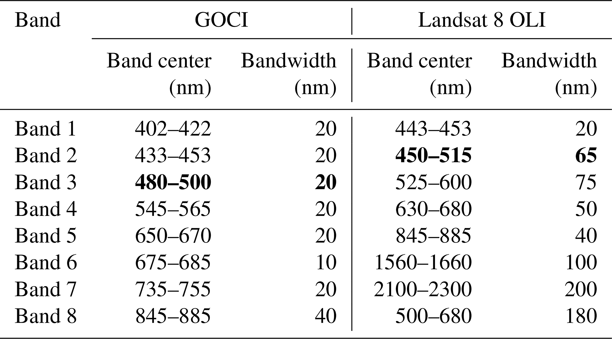
Table 1The comparison of band range between GOCI and Landsat. The selected bands for merging Landsat and GOCI are marked in bold.
2.2 Materials
2.2.1 GOCI
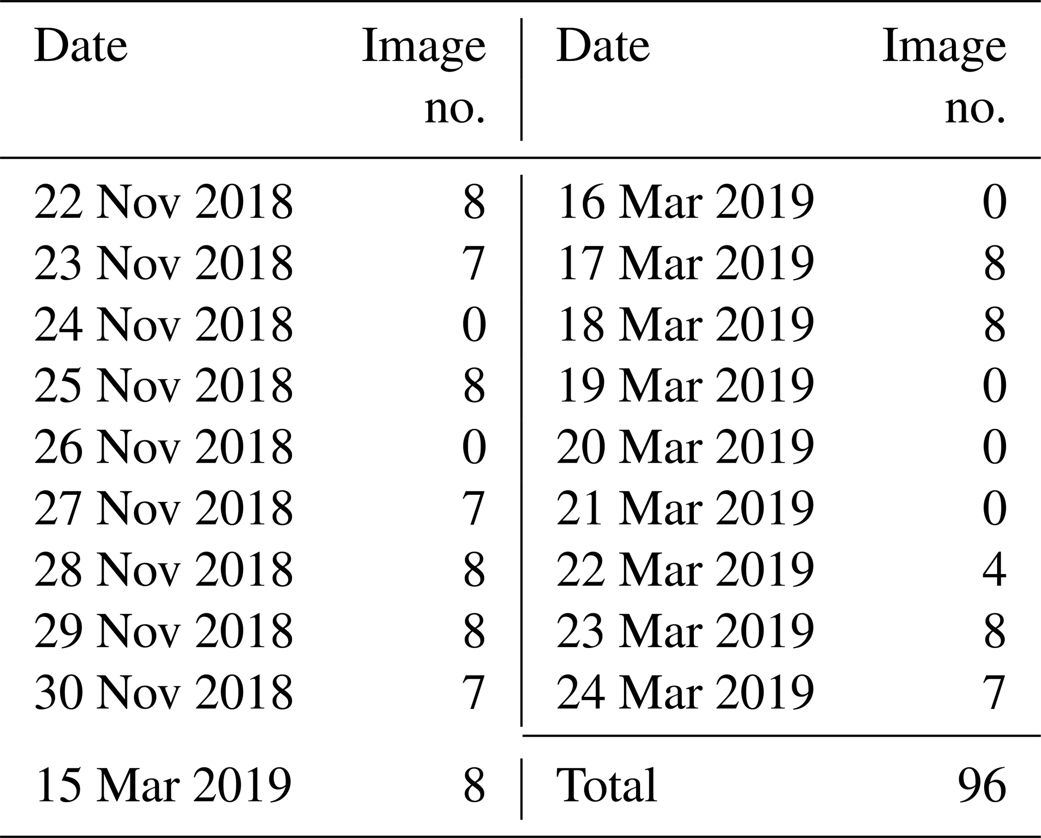
The GOCI is the first satellite for detecting ocean color from a geostationary orbit and has been widely applied in deriving optical, biological, and biogeochemical properties (Ryu et al., 2012; Ryu and Ishizaka, 2012). The GOCI data have been available since April 2004, covering about 2500 km × 2500 km around the Korean Peninsula. It has six visible bands and two near-infrared bands, and Table 1 provides the details of the band information. The GOCI provides observations every hour from 08:30 to 15:30 local time (LT), with a spatial resolution of 500 m. The GOCI has the most significant advantage of a high temporal resolution, with eight images daily, which can offer the details of the freeze-up and break-up processes. A total of 96 GOCI images during the cold season from 2018 to 2019 were used in this study (Table 2). The atmospheric correction was performed by GOCI data processing software (GDPS).
Table 2The usage of GOCI images from November 2018 to March 2019.
2.2.2 Landsat
The Landsat 8 satellite was launched on 11 February 2013. It carries the Operational Land Imager (OLI) and the Thermal Infrared Sensor (TIRS), which have been widely used to monitor lake and river ice (X. Wang et al., 2021; Yang et al., 2020). The OLI has nine bands, with a spatial resolution of 30 m for bands 1–7 and band 9 and a spatial resolution of 15 m for band 8. It has a temporal resolution of 16 d. Six Landsat images taken during the cold season from 2018 to 2019 were prepared for data fusion with the GOCI. The capture dates were 6 November 2018, 22 November 2018, 8 December 2018, 26 February 2019, 14 March 2019, and 15 April 2019. The path and row are 119 and 29, respectively. We downloaded the Landsat-calibrated surface reflectance Tier 1 collection for Landsat 8 OLI (LANDSAT/LC08/C01/T1_SR) from the Google Earth Engine (GEE) for further work. Table 1 compares the band information on Landsat and GOCI. From Table 1, we found that the band range of band 3 from GOCI (480–500 nm) overlapped with that of band 2 from Landsat 8 OLI (450–515 nm). The waterbody had relatively strong reflectance in the blue band (400–480 nm), and the blue band images clearly displayed the linear structure. Therefore, we merged band 3 of the GOCI and band 2 of the Landsat 8 OLI and generated the 96 fusion images for further work.
2.2.3 Auxiliary data
The lake ice phenology of the cold season from 2018 to 2019 was extracted from the combined time series of the surface temperature of lake water provided by the MOD11A1 and MYD11A1 products (Song et al., 2016; Hao et al., 2021). The freeze-up date is defined as the first day on which the surface temperature of lake water is below 0 ∘C in winter; the break-up date is defined as the first day on which the surface temperature of lake water is above 0 ∘C in spring. We utilized the daily air temperatures, precipitation, wind directions, and wind speeds of the Qian'an station (ID 50948) to explain the influence of climate on lake ice from 2010 to 2021. Qian'an has a longitude and latitude of 124.011∘ E and 44.998∘ N, respectively, with an elevation of 146.3 m. In total, 16 directions with an interval of 22.5∘ were used to describe the wind directions, including north (N), north–northeast (NNE), northeast (NE), east–northeast (ENE), east (E), east–southeast (ESE), southeast (SE), south–southeast (SSE), south (S), south–southwest (SSW), southwest (SW), west–southwest (WSW), west (W), west–northwest (WNW), northwest (NW), and north–northwest (NNW). The climate records were used to explain the relationship between lake ice and climate.
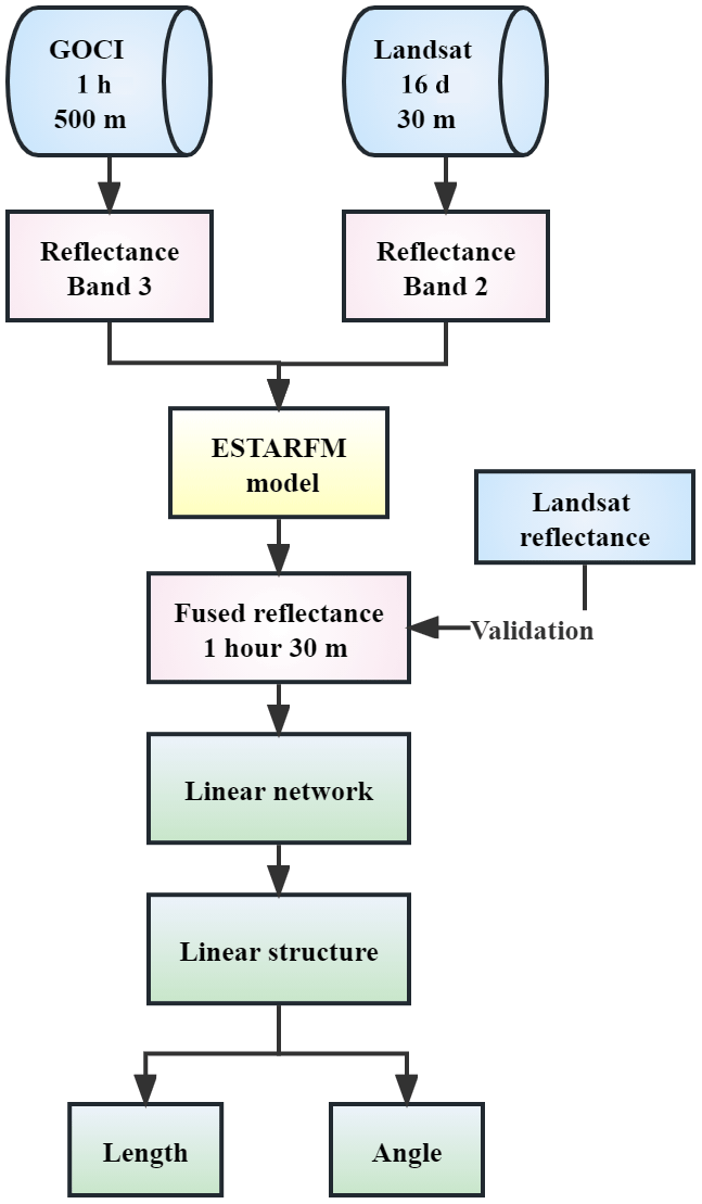
3.1 The framework of methodology
Figure 2 presents the flowchart of our work. We preprocessed the Landsat 8 OLI and GOCI and prepared the reflectance images of band 2 of Landsat 8 OLI and band 3 of GOCI. Then, we merged GOCI and Landsat 8 OLI using the ESTARFM and generated new fusion data with a spatial and temporal resolution of 30 m and 1 h, respectively. After that, the geographic location of the linear structure on the surface of the lake ice was identified, and the morphological parameters were extracted, including lengths and angles.
3.2 The ESTARFM fusion
The ESTARFM, in which two pairs of Landsat and GOCI images were used to generate spatiotemporal fusion data, was proposed by Zhu et al. (2010) and based on the STARFM. First, the coarse GOCI data were projected and resampled to a fine Landsat image at two known times tm and tn. Second, similar neighborhood pixels were searched with a moving window by setting spectral differences. Third, we calculated the normalized weight of each similar pixel by considering the spatial, spectral, and temporal differences. Then, the coarse GOCI values were transferred to fine Landsat data using the pixel-based conversion coefficients in the linear regression. Finally, the coarse GOCI data at the same time were used to calculate the fine fusion data at the predicted time (tp), which is expressed as follows (Liu et al., 2021; Bai et al., 2017; Zhu et al., 2010):
where is the final predicted fine-resolution reflectance at the prediction time tp. w represents the size of the moving window, and the corresponding center is . is the fine-resolution reflectance at tk (k=m or n) at the base date. Tk is the time weight, calculated from the magnitude of the detected change in the reflectance of the coarse spatial-resolution image between tm and tn and the prediction moment tp.
where C(xj, yi, tk) and denote the image element values of similar image elements (xi,yj) within the moving window of the coarse spatial-resolution image at the reference moment tk and prediction moment tp, respectively.
3.3 The quantitative analysis of linear structures
In the beginning, the Landsat-GOCI fusion images were transformed into binary images. We extracted the original linear network with the Canny (1986) edge detection algorithm and then conducted edge detection to remove the outer boundaries. The morphological processing, including opening, filling, and eroding sequentially, was implemented for the inner part of the linear network. Then, the linear structure was derived from the largest connected domain of the linear network without boundaries, and the length is calculated by the shortest path of the largest connected domain. We connected the northernmost and southernmost ends into a straight line. The angle followed the definition of the wind direction above. We compared the auto-extraction and visual interpretation in our previous work (Hao et al., 2021). The R2 values of the length and angle of 0.96 and 0.98 proved the good performance of the auto-extraction algorithm.
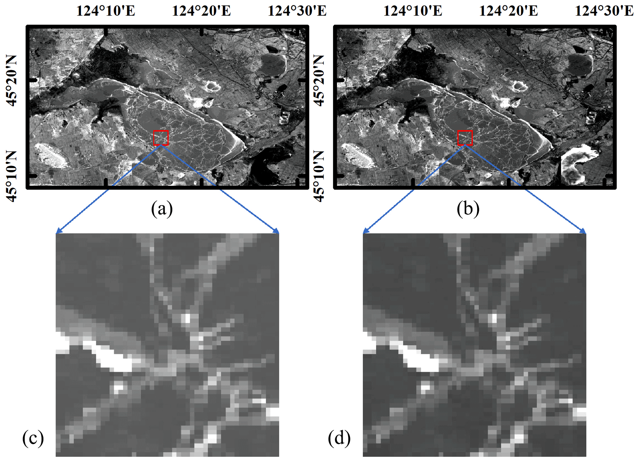
Figure 3The actual image observed on 22 November 2018 (a) and its prediction images by the ESTARFM (b). Panels (c) and (d) display the magnified version of the red rectangle in panels (a) and (b), respectively.
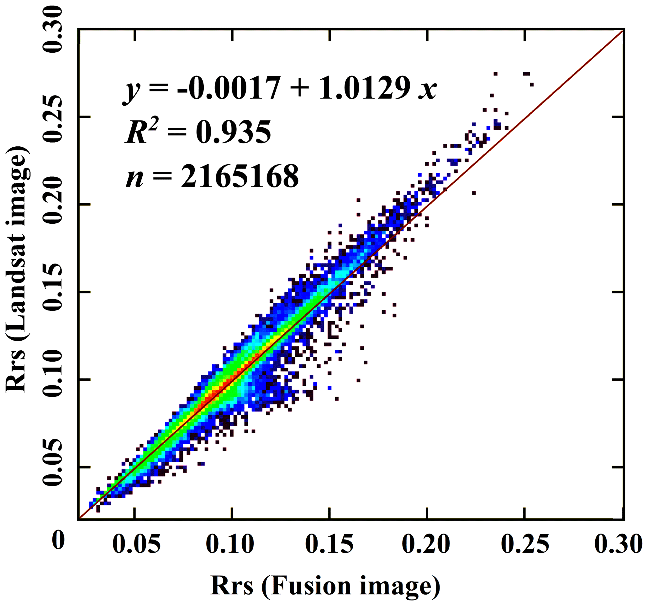
Figure 4Scatterplot of the real and the predicted reflectance by the ESTARFM for the blue band. The capture date was 22 November 2018.
4.1 The performance of ESTARFM
We predicted the fine images from two pairs of fine Landsat and coarse GOCI data to fill the data gap caused by the low revisit frequency of Landsat. The two known pairs of data in the freeze-up process were captured on 6 November and 8 December 2018, and 53 fine ESTARFM fusion images were predicted from the coarse GOCI images. The two known pairs of data of the break-up process were captured on 26 February and 15 April 2019, and 43 fine ESTARFM fusion images were predicted. Figure 3 compares the spatial distribution of the original images and predicted images on 22 November 2018. In the predicted images, the texture of the ground objects was maintained, and the magnified versions of the figures in Fig. 3c and d clearly display the distribution of the linear structure. The predicted images were consistent with the original images and indicated the good fusion effect of ESTARFM. Figure 4 illustrates the scatterplots of the actual and predicted reflectance values along the 1:1 line. The R2 value is 0.935, indicating that the predicted image was highly correlated with the actual image. The ranges of predicated and actual images were consistent; their mean reflectance values were both 0.10±0.03. The performance of the ESTARFM results was limited by (1) the limited image pairs available during the cold season from 2018 to 2019, (2) the time lag between the predicted and actual images, and (3) the inconsistency of the capture time between the predicted images and two pairs of input images (Lu et al., 2019; M. Liu et al., 2018). Therefore, the ESTARFM fusion images had a good performance and can provide reliable materials for further exploration.
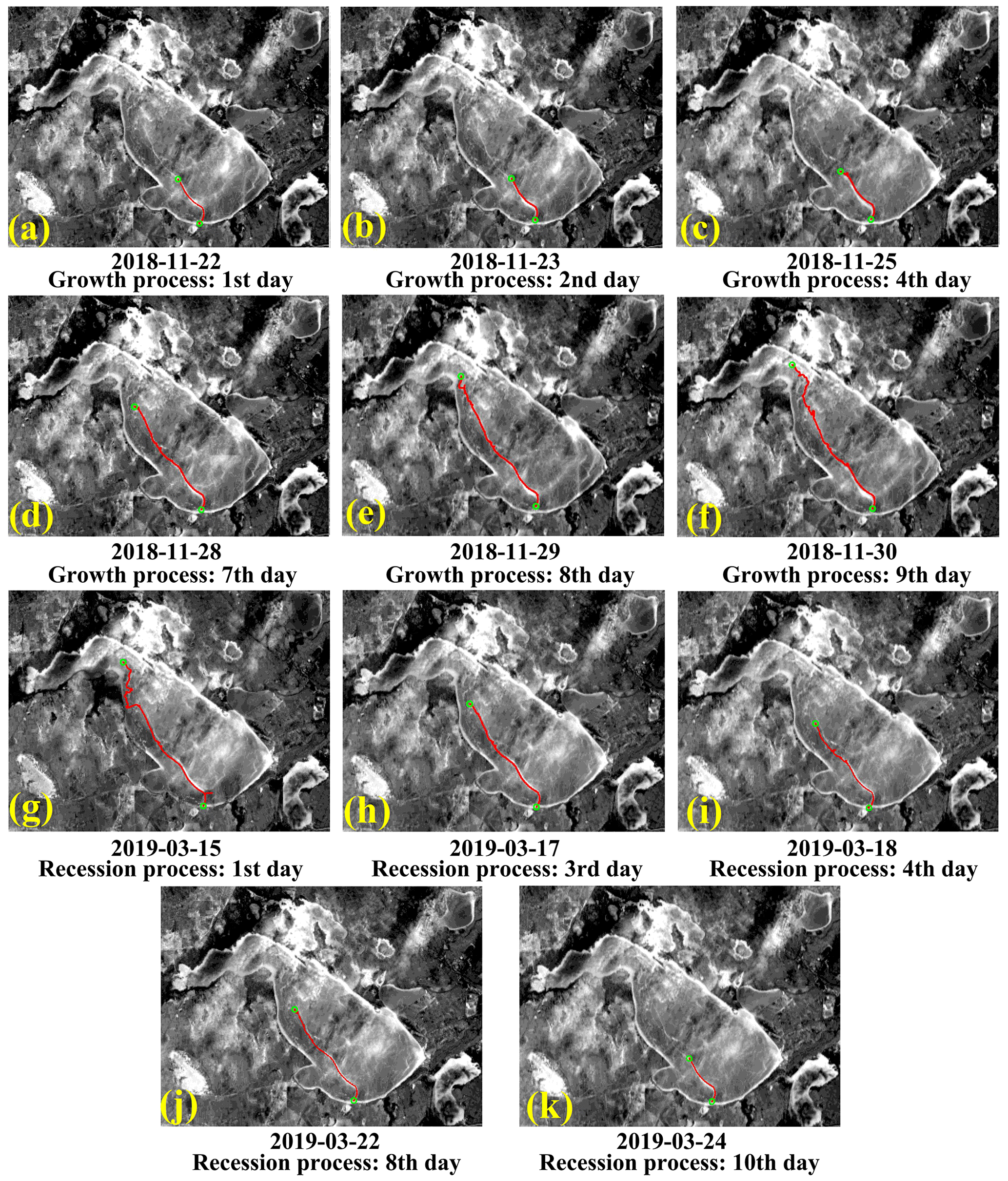
Figure 5The spatiotemporal changes in the linear structure for the fusion images of Lake Chagan during the cold season of 2018–2019.
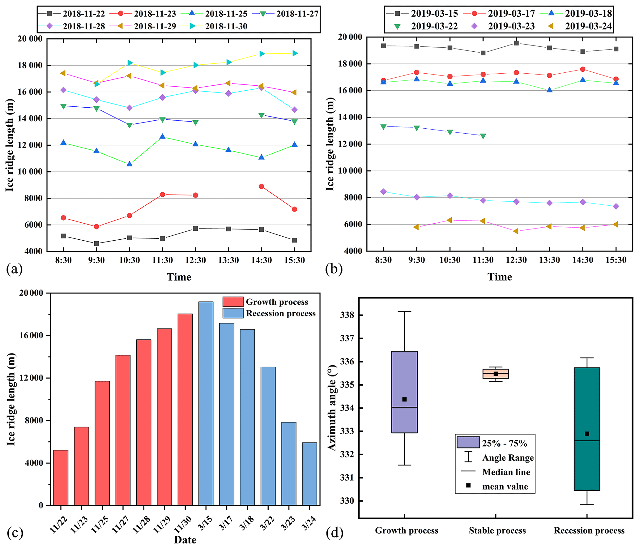
Figure 6The changes in the ice ridges during the cold season of 2018–2019. (a) Length changes during the growth process from 22 to 30 November 2018, as measured from 53 ESTARFM fusion images. (b) Length changes during the recession process from 15 to 24 March 2019, as measured from 43 ESTARFM fusion images. (c) The daily average length. (d) The angles of ice ridges in different stages.
4.2 The changes in surface morphology
We extracted the surface morphology of Chagan Lake from 96 fusion images during the cold season from 2018 to 2019. Figure 5 displays the spatial changes in the linear structure of the Landsat images in the freeze-up and break-up processes. Figures A1 and A2 present the original images of the GOCI, with a resolution of 500 m, the fusion images of Landsat and GOCI, with a spatial resolution of 30 m, and the network structure and the linear structure in the freeze-up and break-up processes, thus providing more details of the extraction process. The linear structure appeared on images from southeast to northwest, lasting from 22 to 30 November 2018. The linear structure disappeared from northwest to southeast, lasting from 15 to 24 March 2019. Figure 6 shows the average daily lengths of the ice ridges, based on the Landsat and GOCI remote sensing data. We monitored the growth and recession process of the linear structure via 96 Landsat-GOCI fusion images and monitored the stable process via four Landsat images. The growth stage lasted for 9 d, from 22 to 30 November 2018. The ice ridges had a length range of 5211.17–18 042.15 m and an average value of 12 680.32±4472.37 m, extending from southeast to northwest. The azimuth angles of the ice ridges in the growth stage ranged from 331.54 to 338.17∘, with an average value of 334.38∘ ± 2.08∘. The lengths in the stable process ranged from 21 052.78 to 21 227.53 m, with an average value of 21 141.57±68.26 m, and the angles changed from 335.15 to 335.77∘, with an average value of 335.48±0.20∘. The recession stage lasted for 10 d, from 15 to 24 March 2019. The ice ridges had a length range of 19 178.18–5924.03 m and an average value of 13 288.59±4907.89 m, disappearing from northwest to southeast. The azimuth angles of the ice ridges in the recession stage ranged from 329.84 to 336.16∘, with an average value of 332.90∘ ± 2.54∘. The changing rates in the growth and recession stages were 1425.66 and 1325.42 m per day, respectively, indicating that growth was slightly faster than recession. The large-scale structure extending from northwest to southeast has repeatedly appeared on Landsat images since 1986, which has been reported in our previous work (Hao et al., 2021).
4.3 The field investigation
Considering the safety of traveling on ice, we conducted two field investigations during the two recent cold seasons, from 30 to 31 December 2020 and 2 to 4 January 2022, respectively. We divided the lake area into three regions according to the surface morphology of lake ice. Region 1 was distributed along the linear structures. The surface of lake ice is uneven, and ice fractures and ice ridges were widely distributed. Region 2 was distributed along the northeastern coast, where the Ice and Snow Fishing and Hunting Cultural Tourism Festival of Chagan Lake has been held at the end of December each year since 2001. Region 3 covered the southern part of Chagan Lake. The lake ice in Regions 2 and 3 was flat and smooth, and snow cover was sporadically distributed. The color of the lake ice along the linear structure was distinguished from lake ice in the neighborhood. We infer that the frozen time of the linear structure was later than the lake ice in the neighborhood. The difference between ice fractures and ice ridges was the vertical height. Ice ridges were elevated sections formed on the upper and lower surfaces of lake ice, consisting mainly of ridge sails and keels. We located 10 sampling points along the linear structure on the satellite images and collected field photos of ice ridges and fractures (Fig. 1). We further verified that the large-scale fractures on the images were made up of ice fractures and ridges.

Figure 7The ice thickness (mm) and water depth (m) of Chagan Lake was measured during the periods from 2 to 4 January 2022.
We also measured the ice thicknesses and water depths of 16 sampling points (Fig. 7). The ice thicknesses in the winter of 2021 ranged from 437.55 to 668.25 mm, with an average value of 582.24±58.14 mm. The average ice thicknesses of Regions 1, 2, and 3 were 551.58, 547.75, and 645.74 mm, respectively. The average water depths of Regions 1, 2, and 3 were 3.48, 2.99, and 3.00 m, respectively. Among the three regions, Region 2 had the smallest average values of ice thickness and water depth. The differences in water depth between the fall of 2021 and the winner of 2021 had an average value of 0.12±0.05 m and a maximum value of 0.2 m. The water depth in winter was lower than that in fall, and the decreasing water level also was a cause of lake ice fracturing in winter (Leppäranta, 2015). The ice features first formed in the nearshore area of the southeastern coast, where the water depth was relatively smaller than that in other regions in Fig. 7. The ice thicknesses and water depths showed spatial coherence with the surface morphology.
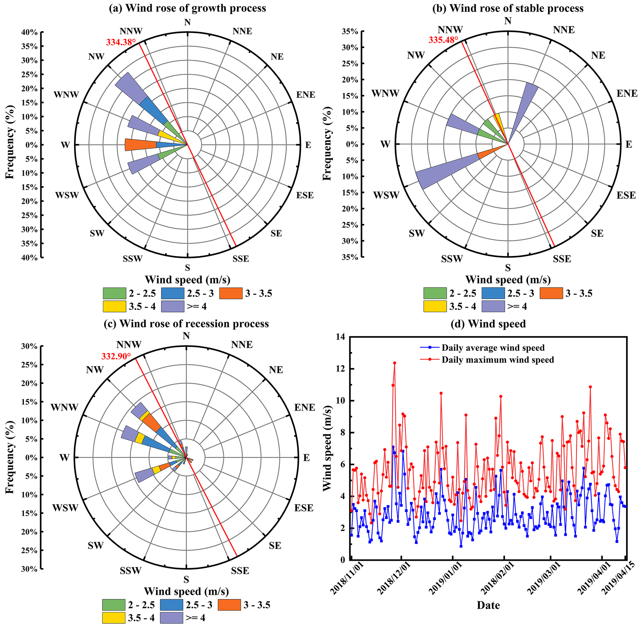
Figure 8The wind field of Chagan Lake during the cold season of 2018. (a) Growth process from 22 to 30 November 2018. (b) Stable process. (c) Recession process from 15 to 24 March 2019. (d) Daily average and maximum wind speed from 1 November 2018 to 15 April 2019.
4.4 The climate condition
Lake ice processes are governed by the complex interaction of hydraulics, thermodynamics, and mechanics. The heat loss due to the decreasing air temperature exceeds the heat gained from surface water in late fall and early winter. When the water temperature falls below the freezing point, the cooled water provides a beneficial condition for ice crystals. Then, the volume of the lake ice expands, and the amount increases, which is followed by the formation of ice. We analyzed the wind roses of the daily average and maximum wind speeds from 1 November 2018 to 15 April 2019 (Fig. 8). The freeze-up and break-up dates of Chagan Lake in the cold season of 2019 derived from MODIS daily land surface temperature (LST) products were 14 November 2018 and 24 March 2019, respectively. The ice ridges appeared on 22 November 2018, 5 d after the freeze-up date; they disappeared on 24 March 2019 and were consistent with the break-up date.
The domain wind in the growth process was NW, WNW, W, and WSW, the domain wind in the stable process was WNW, WSW, and NNE, and the domain wind in the recession process was NW, WNW, and WSW. The WNW and WSW direction was the domain wind direction for all three stages. The frequency in the WSW direction in the growth, stability, and recession stages was 22.22 %, 30 %, and 14.23 %, respectively. The angles between the WSW direction and ice ridges were 87.98, 86.88, and 85.40∘ for the three stages. The nearly perpendicular relationship was consistent with our previous study (Hao et al., 2021). Our previous used the yearly average values of wind from 2013 and 2020, and the work herein just exploited the wind in the cold season from 2018 to 2019. Besides, the wind speed also contributed to the formation of ice cracks and ridges. The daily average wind speed in the growth process and recession process was 3.88 and 3.63 m s−1, and the average values for the whole cold season were 2.97 m s−1. The daily maximum wind speeds for both the growth process and recession process were 3.88, 3.63, 7.05, and 6.86 m s−1, and the average value for the whole cold season was 5.65 m s−1. Not only the daily average value but also the maximum value was higher than the average level and revealed that the changing processes of ice fractures and ridges require the relatively strong action of wind. Therefore, wind speeds and directions played crucial roles in the development of ice ridges.
Lake ice experiences different stages during the freezing and thawing cycle, including the phases of ice crystals, frazil ice, nails, pancake ice, and ice layers (Leppäranta, 2015). Lake ice expands and contracts as the air temperature rises and drops during cold seasons. The temperature difference between night and day results in the thermal expansion and contract of lake ice, which differ significantly within a given lake. Furthermore, long and narrow cracks are generated and likely to evolve into ice ridges under pressure when lake ice bulks, collides, and piles up. The definitions of lake ice are limited by the view ranges of field measurements, and satellite remote sensing provides a new perspective for surface morphology in a larger-scale observation. The large-scale linear structure has been found on remote sensing images during the cold season from 2018 to 2019. Similar phenomena have also been found in lakes and reservoirs in Northeast China (X. Liu et al., 2018). In our previous work, we used four Landsat 8 OLI images to monitor the monthly changes due to the limitation of temporal resolution (Hao et al., 2021). In this study, we took advantage of the hourly revisit of the GOCI and generated 53 and 43 ESTARFM fusion images in the freeze-up and break-up processes, respectively. This makes it possible to explore the linear structure in detail. The recurrent large-scale linear structure was further verified as being ice fractures and ice ridges in the fieldwork. Determining the spatial scales of ice fractures and ice ridges is challenging work, when considering the data source. A UAV is suitable to monitor the lake ice fractures at small scales (0–100 m), and the satellite sensors are suitable to monitor the ice ridges at large scales (10–100 km); both are suitable to monitor the horizon changes in the lake ice surface.
Besides the thermal forces, the lake ice fractures and ridges are also a dynamic process under the control of mechanical forces. The wind above the ice covers and water currents beneath the ice covers force the shift in ice bulk (Tan et al., 2012). Wang et al. (2006) compared the mechanical changes in the leads and ice covers, based on modeling results and satellite monitoring (Wang et al., 2006; Leppäranta, 2010), and revealed the influence of winds on the drift of ice. In the freeze-up process, the winds and water currents can push the ice toward the shore, preventing ice covers from freezing; in the break-up process, the wind can break ice covers and accelerate melting. The lake ice fractures were mainly controlled by thermal forces, and the ice ridges were mainly controlled by mechanical forces. The ice ridges underwent three stages during the cold season of 2018–2019, in which the wind directions and speeds exhibited remarkable differences. The ice ridges grew from southeast to northwest, with an average direction of 334.38∘ and decayed from northwest to southeast with an average direction of 332.90∘. The WSW direction frequently happened in all three stages, revealing the crucial role of winds in the development of ice ridges. The direction of the ice ridges was nearly perpendicular to the WSW direction (247.5∘), which followed the principal laws of mechanics. The air temperature created a cold environment for the ice cover to freeze, the wind provided a mechanical force for the ice bulk to shift, and ice ridges and ice fractures formed. In addition, the direction of the ice ridges had a similar shape to the southwestern shoreline, and the stable shoreline geometry could explain the recurrent ice ridges with a specific direction, which has been reported in previous studies (Leppäranta, 2015).
Linear structures are common natural phenomena on the surfaces of sea ice and lake ice and profoundly influence light transfer and ice ecology. Lake ice ridges alter surface roughness and light transfer and then contribute to the thickness and volume of ice. People in cold regions have skillfully taken advantage of frozen ice covers for fishing, food storage, and commercial transportation. The capacity and stability of floating ice can be evaluated by the ice thickness and the spatial distribution of ice fractures and ridges (Tan et al., 2012). Generally, 30 cm is the thickness suggested for safe human activities on the ice (Leppäranta, 2015). Ice fractures and ice ridges potentially threaten human activities. In field investigations, we measured the ice thicknesses along the linear structure when the ice covers were steady. The ice thicknesses along the ice ridges were supposed to be thinner than in other areas (Leppäranta, 2015), but no significant difference in ice thickness had been found in our field measurements. Thus, the surface morphology of lake ice would be a reliable sign of travel on the ice being dangerous. Besides, we monitored the horizon changes in lake ice ridges using optical satellite images but ignored the vertical heights of ice ridges, which we need to consider in future work.
We generated high spatiotemporal remote sensing data of Landsat and GOCI, using ESTARFM to fill the gap in the fine monitoring of lake ice dynamics in Lake Chagan. We compared the reflectance of the fusion images and the original images on 22 November 2018. The R2 value between the actual images and predicted images is up to 0.935, indicating that the predicted images were highly correlated with the actual images. Moreover, the consistency of the texture of the ground objects was maintained between the predicted images and the original images. Therefore, the ESTARFM fusion images provided reliable materials for further exploration.
We calculated the lengths and the angles of the linear structure on the fusion images in the freeze-up and break-up processes during the cold season from 2018 to 2019. Based on the satellite images, the linear structure experienced growth, stability, and recession stages. The growth stage lasted for 9 d, ranging from 22 to 30 November 2018. The recession stage lasted for 10 d, ranging from 15 to 22 March 2019. From southeast to northwest, the linear structure was 5211.17 to 18 042.15 m long during growth and from northwest to southwest, it disappeared. The average length of the ice ridges in the completely frozen period was 21 141.57±68.36 m. The average azimuth angle was 335.48∘ ± 0.23∘.
We performed field investigations and verified the linear structure as ice fractures and ridges. The direction of the linear structure was nearly perpendicular to the southwesterly wind direction, which is the dominant wind direction in winter. The deformation of the surface morphology was related to the meteorological conditions before the freeze-up process, including winds and air temperatures. This work demonstrated the capability of monitoring large-scale surface morphology using multi-source remote sensing and has profound implications for traveling safety on ice and ice engineering. We also plan to extend our findings to other large lakes in China and fill the knowledge gap of the surface morphology of lake ice.
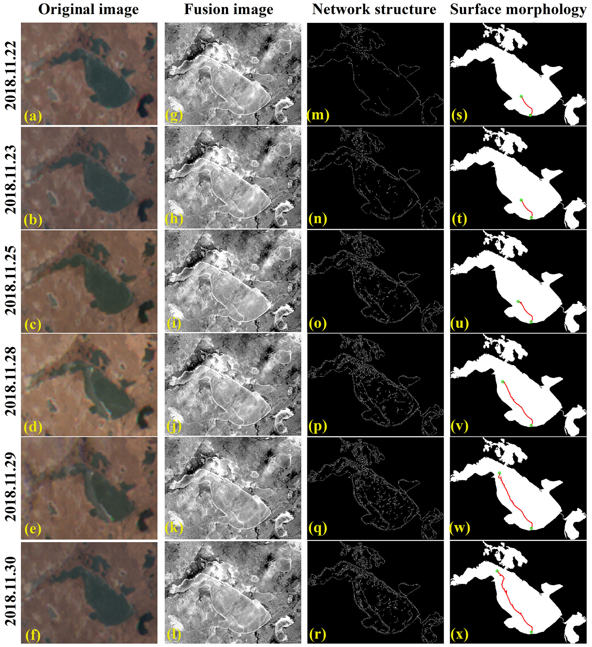
Figure A1The changes in ice ridges during the freeze-up process from 22 to 30 November 2019. (a–f) The original images from GOCI. (g–l) The fusion images from Landsat and GOCI. (m–r) The network structure of surface morphology. (s–x) The surface morphology.
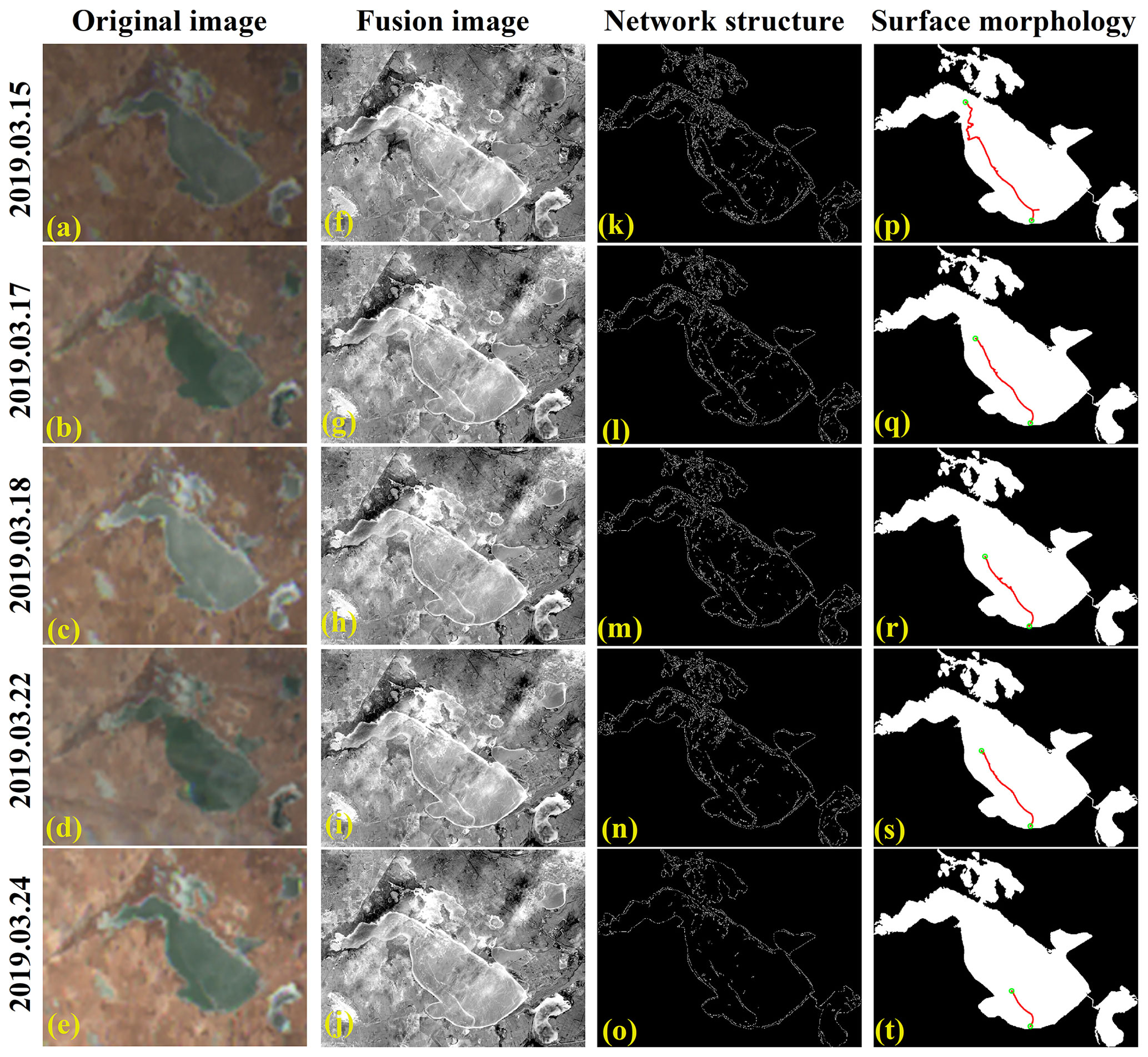
Figure A2The changes in ice ridges during the break-up process from 15 to 24 March 2019. (a–e) The original images from GOCI. (f–j) The fusion images from Landsat and GOCI. (k–o) The network structure of surface morphology. (p–t) The surface morphology.
All raw data and code can be provided by the corresponding author upon request.
QY, FX, and ZL planned the field investigation. XS and WL processed the remote sensing data. CF and NL analyzed the data. QY and KS wrote the draft. XH, ZL, ZW, and GL reviewed and edited the paper.
The contact author has declared that none of the authors has any competing interests.
Publisher's note: Copernicus Publications remains neutral with regard to jurisdictional claims in published maps and institutional affiliations.
The authors would like to thank the KORDI/KOSC, for providing GOCI data, the GEE platform, for providing MODIS and Landsat data, and the China Meteorological Data Sharing Service System, for climate records. Thanks are given to our students Feng Tao, Xuan Li, and Kenan Sun, for helping with the field investigation. The comments from the reviewers, which improved the quality of this work, are greatly appreciated.
This research has been jointly supported by the Scientific and Technological Development Project (grant no. YDZJ202301ZYTS212), 14th Five-Year Plan of Technical and Social Research Project for Jilin Colleges of China (grant no. JJKH20210290KJ), the National Natural Science Foundation of China (grant no. 41971325), the National Key Research and Development Program of China (grant no. 2019YFE0197600).
This paper was edited by Homa Kheyrollah Pour and reviewed by Xiaoyan Wang and one anonymous referee.
Arp, C. D., Cherry, J. E., Brown, D. R. N., Bondurant, A. C., and Endres, K. L.: Observation-derived ice growth curves show patterns and trends in maximum ice thickness and safe travel duration of Alaskan lakes and rivers, The Cryosphere, 14, 3595–3609, https://doi.org/10.5194/tc-14-3595-2020, 2020.
Bai, L., Cai, J., Liu, Y., Chen, H., Zhang, B., and Huang, L.: Responses of field evapotranspiration to the changes of cropping pattern and groundwater depth in large irrigation district of Yellow River basin, Agr. Water. Manage., 188, 1–11, https://doi.org/10.1016/j.agwat.2017.03.028, 2017.
Bojinski, S., Verstraete, M., Peterson, T. C., Richter, C., Simmons, A., and Zemp, M.: The concept of essential climate variables in support of climate research, applications, and policy, B. Am. Meteorol. Soc., 95, 1431–1443, https://doi.org/10.1175/bams-d-13-00047.1, 2014.
Brown, L. C. and Duguay, C. R.: The response and role of ice cover in lake-climate interactions, Prog. Phys. Geog., 34, 671–704, https://doi.org/10.1177/0309133310375653, 2010.
Cai, Y., Ke, C. Q., and Duan, Z.: Monitoring ice variations in Qinghai Lake from 1979 to 2016 using passive microwave remote sensing data, Sci. Total Environ., 607, 120–131, https://doi.org/10.1016/j.scitotenv.2017.07.027, 2017.
Cai, Y., Ke, C. Q., Li, X., Zhang, G., Duan, Z., and Lee, H.: Variations of lake ice phenology on the Tibetan Plateau from 2001 to 2017 based on MODIS data, J. Geophys. Res.-Atmos., 124, 825–843, https://doi.org/10.1029/2018jd028993, 2019.
Canny, J.: A computational approach to edge detection, IEEE T. Pattern Anal., 8, 679–698, 1986.
Dierking, W.: Mapping of different sea ice regimes using images from Sentinel-1 and ALOS synthetic aperture radar, IEEE T. Geosci. Remote., 48, 1045–1058, https://doi.org/10.1109/TGRS.2009.2031806, 2010.
Doernhoefer, K. and Oppelt, N.: Remote sensing for lake research and monitoring – Recent advances, Ecol. Indic., 64, 105–122, https://doi.org/10.1016/j.ecolind.2015.12.009, 2016.
Du, J., Kimball, J. S., Duguay, C., Kim, Y., and Watts, J. D.: Satellite microwave assessment of Northern Hemisphere lake ice phenology from 2002 to 2015, The Cryosphere, 11, 47–63, https://doi.org/10.5194/tc-11-47-2017, 2017.
Du, J., Watts, J. D., Jiang, L., Lu, H., Cheng, X., Duguay, C., Farina, M., Qiu, Y., Kim, Y., Kimball, J. S., and Tarolli, P.: Remote sensing of environmental changes in cold regions: Methods, achievements and challenges, Remote. Sens., 11, 1592, https://doi.org/10.3390/rs11161952, 2019.
Duan, H., Zhang, Y., Zhang, B., Song, K., and Wang, Z.: Assessment of chlorophyll-a concentration and trophic state for Lake Chagan using Landsat TM and field spectral data, Environ. Monit. Assess., 129, 295–308, https://doi.org/10.1007/s10661-006-9362-y, 2007.
Feng, G., Masek, J., Schwaller, M., and Hall, F.: On the blending of the Landsat and MODIS surface reflectance: predicting daily Landsat surface reflectance, IEEE T. Geosci. Remote., 44, 2207–2218, https://doi.org/10.1109/tgrs.2006.872081, 2006.
Geldsetzer, T., Sanden, J. V. D., and Brisco, B.: Monitoring lake ice during spring melt using RADARSAT-2 SAR, Can. J. Remote Sens., 36, S391–S400, 2010.
Gogineni, P. and Yan, J.-B.: Remote sensing of ice thickness and surface velocity, in: Remote Sensing of the Cryosphere, edited by: Tedesco, M., John Wiley & Sons, Ltd., https://doi.org/10.1002/9781118368909.ch9, 2015.
Gusmeroli, A. and Grosse, G.: Ground penetrating radar detection of subsnow slush on ice-covered lakes in interior Alaska, The Cryosphere, 6, 1435–1443, https://doi.org/10.5194/tc-6-1435-2012, 2012.
Hampton, S. E., Galloway, A. W., Powers, S. M., Ozersky, T., Woo, K. H., Batt, R. D., Labou, S. G., O'Reilly, C. M., Sharma, S., Lottig, N. R., Stanley, E. H., North, R. L., Stockwell, J. D., Adrian, R., Weyhenmeyer, G. A., Arvola, L., Baulch, H. M., Bertani, I., Bowman, L. L., Jr., Carey, C. C., Catalan, J., Colom-Montero, W., Domine, L. M., Felip, M., Granados, I., Gries, C., Grossart, H. P., Haberman, J., Haldna, M., Hayden, B., Higgins, S. N., Jolley, J. C., Kahilainen, K. K., Kaup, E., Kehoe, M. J., MacIntyre, S., Mackay, A. W., Mariash, H. L., McKay, R. M., Nixdorf, B., Noges, P., Noges, T., Palmer, M., Pierson, D. C., Post, D. M., Pruett, M. J., Rautio, M., Read, J. S., Roberts, S. L., Rucker, J., Sadro, S., Silow, E. A., Smith, D. E., Sterner, R. W., Swann, G. E., Timofeyev, M. A., Toro, M., Twiss, M. R., Vogt, R. J., Watson, S. B., Whiteford, E. J., and Xenopoulos, M. A.: Ecology under lake ice, Ecol. Lett., 20, 98–111, https://doi.org/10.1111/ele.12699, 2017.
Hao, X., Yang, Q., Shi, X., Liu, X., Huang, W., Chen, L., and Ma, Y.: Fractal-based retrieval and potential driving factors of lake ice fractures of Chagan Lake, Northeast China using Landsat remote sensing images, Remote Sens., 13, 4233, https://doi.org/10.3390/rs13214233, 2021.
Hilker, T., Wulder, M. A., Coops, N. C., Linke, J., McDermid, G., Masek, J. G., Gao, F., and White, J. C.: A new data fusion model for high spatial- and temporal-resolution mapping of forest disturbance based on Landsat and MODIS, Remote Sens. Environ., 113, 1613–1627, https://doi.org/10.1016/j.rse.2009.03.007, 2009.
Hoekstra, M., Jiang, M., Clausi, D. A., and Duguay, C.: Lake ice-water classification of RADARSAT-2 images by integrating IRGS Segmentation with pixel-based random forest labeling, Remote Sens., 12, 1425, https://doi.org/10.3390/rs12091425, 2020.
Howell, S. E. L., Brown, L. C., Kang, K.-K., and Duguay, C. R.: Variability in ice phenology on Great Bear Lake and Great Slave Lake, Northwest Territories, Canada, from SeaWinds/QuikSCAT: 2000–2006, Remote Sens. Environ., 113, 816–834, https://doi.org/10.1016/j.rse.2008.12.007, 2009.
IPCC: Climate change 2021: The physical science basis., Contribution of Working Group I to the Sixth Assessment Report of the Intergovernmental Panel on Climate Change, https://iupac.org/climate-change-2021-the-physical-science-basis/ (last access: 16 February 2022), 2021.
Jarihani, A., McVicar, T., Van Niel, T., Emelyanova, I., Callow, J., and Johansen, K.: Blending Landsat and MODIS data to generate multispectral indices: A comparison of “Index-then-Blend” and “Blend-then-Index” approaches, Remote Sens., 6, 9213–9238, https://doi.org/10.3390/rs6109213, 2014.
Jeffries, M. O., Morris, K., and Kozlenko, N.: Ice characteristics and processes, and remote sensing of frozen rivers and lakes, in: Remote Sensing in Northern Hydrology: Measuring Environmental Change, edited by: Pietroniro, C. R. D. A., https://doi.org/10.1029/GM163, 2013.
Jones, B. M., Gusmeroli, A., Arp, C. D., Strozzi, T., Grosse, G., Gaglioti, B. V., and Whitman, M. S.: Classification of freshwater ice conditions on the Alaskan Arctic Coastal Plain using ground penetrating radar and TerraSAR-X satellite data, Int. J. Remote Sens., 34, 8267–8279, https://doi.org/10.1080/2150704X.2013.834392, 2013.
Kang, K.-K. K., Duguay, C. R., Lemmetyinen, J., and Gel, Y.: Estimation of ice thickness on large northern lakes from AMSR-E brightness temperature measurements, Remote Sens. Environ., 150, 1–19, 2014.
Ke, C.-Q., Tao, A.-Q., and Jin, X.: Variability in the ice phenology of Nam Co Lake in central Tibet from scanning multichannel microwave radiometer and special sensor microwave/imager: 1978 to 2013, J. Appl. Remote. Sens., 7, 073477, https://doi.org/10.1117/1.Jrs.7.073477, 2013.
Knauer, K., Gessner, U., Fensholt, R., and Kuenzer, C.: An ESTARFM fusion framework for the generation of large-scale time series in cloud-prone and heterogeneous landscapes, Remote. Sens., 8, 425, https://doi.org/10.3390/rs8050425, 2016.
Lang, J., Lyu, S., Li, Z., Ma, Y., and Su, D.: An investigation of ice surface albedo and its influence on the high-altitude lakes of the Tibetan Plateau, Remote. Sens., 10, 218, https://doi.org/10.3390/rs10020218, 2018.
Leppäranta, M.: Modelling the formation and decay of lake ice, in: The Impact of Climate Change on European Lakes, edited by: George, G., Springer Netherlands, Dordrecht, 63–83, https://doi.org/10.1007/978-90-481-2945-4_5, 2010.
Leppäranta, M.: Freezing of lakes and the evolution of their ice cover, Springer Science & Business Media, https://doi.org/10.1007/978-3-642-29081-7, 2015.
Li, W., Lu, P., Li, Z., Zhuang, F., Lu, Z., and Li, G.: Analysis of ice cracks morphology on lake surface of Lake Wuliangsuhai in the winter of 2017–2018, J. Glaciol. Geocry., 42, 919–926, https://doi.org/10.7522/j.issn.1000-0240.2020.0066, 2020 (in Chinese).
Li, Z., Ao, Y., Lyu, S., Lang, J., Wen, L., Stepanenko, V., Meng, X., and Zhao, L. I. N.: Investigation of the ice surface albedo in the Tibetan Plateau lakes based on the field observation and MODIS products, J. Glaciol., 64, 506–516, https://doi.org/10.1017/jog.2018.35, 2018.
Liu, C., Duan, P., Zhang, F., Jim, C.-Y., Tan, M. L., and Chan, N. W.: Feasibility of the spatiotemporal fusion model in monitoring Ebinur Lake's suspended particulate matter under the missing-data scenario, Remote Sens., 13, 3952, https://doi.org/10.3390/rs13193952, 2021.
Liu, M., Liu, X., Wu, L., Zou, X., Jiang, T., and Zhao, B.: A modified spatiotemporal fusion algorithm using phenological information for predicting reflectance of paddy Rice in Southern China, Remote Sens., 10, 772, https://doi.org/10.3390/rs10050772, 2018.
Liu, X., Li, B., Li, Z., and Shen, W.: A new fracture model for reservoir ice layers in the northeast cold region of China, Constr. Build. Mater., 191, 795–811, https://doi.org/10.1016/j.conbuildmat.2018.10.050, 2018.
Liu, X., Zhang, G., Sun, G., Wu, Y., and Chen, Y.: Assessment of Lake water quality and eutrophication risk in an agricultural irrigation area: A case study of the Chagan Lake in Northeast China, Water, 11, 2380, https://doi.org/10.3390/w11112380, 2019.
Liu, X., Zhang, G., Zhang, J., Xu, Y. J., Wu, Y., Wu, Y., Sun, G., Chen, Y., and Ma, H.: Effects of irrigation discharge on salinity of a large freshwater lake: A case study in Chagan Lake, Northeast China, Water, 12, 2112, https://doi.org/10.3390/w12082112, 2020.
Lu, Y., Wu, P., Ma, X., and Li, X.: Detection and prediction of land use/land cover change using spatiotemporal data fusion and the Cellular Automata–Markov model, Environ. Monit. Assess., 191, 68, https://doi.org/10.1007/s10661-019-7200-2, 2019.
Magnuson, J. J., Robertson, D. M., Benson, B. J., Wynne, R. H., Livingstone, D. M., Arai, T., Assel, R. A., Barry, R. G., Card, V., Kuusisto, E., Granin, N. G., Prowse, T. D., Stewart, K. M., and Vuglinski, V. S.: Historical trends in lake and river ice cover in the Northern Hemisphere, Science, 289, 1743–1746, https://doi.org/10.1126/science.289.5485.1743, 2000.
Murfitt, J. and Duguay, C. R.: Assessing the performance of methods for monitoring ice phenology of the world's largest high Arctic lake using high-density time series analysis of Sentinel-1 data, Remote Sens., 12, 382, https://doi.org/10.3390/rs12030382, 2020.
Murfitt, J. and Duguay, C. R.: 50 years of lake ice research from active microwave remote sensing: Progress and prospects, Remote Sens. Environ., 264, 112616, https://doi.org/10.1016/j.rse.2021.112616, 2021.
Murfitt, J., Brown, L. C., and Howell, S. E. L.: Evaluating RADARSAT-2 for the monitoring of lake ice phenology events in mid-latitudes, Remote Sens., 10, 1641, https://doi.org/10.3390/rs10101641, 2018a.
Murfitt, J. C., Brown, L. C., and Howell, S. E.: Estimating lake ice thickness in Central Ontario, Plos one, 13, e0208519, https://doi.org/10.1371/journal.pone.0208519, 2018b.
Qi, M., Liu, S., Yao, X., Xie, F., and Gao, Y.: Monitoring the ice phenology of Qinghai Lake from 1980 to 2018 using multisource remote sensing data and Google Earth Engine, Remote Sens, 12, 2217, https://doi.org/10.3390/rs12142217, 2020.
Qiu, Y., Wang, X., Ruan, Y., Xie, P., Zhong, Y., and Yang, S.: Passive microwave remote sensing of lake freeze-thawing over Qinghai-Tibet Plateau, J. Lake. Sci., 30, 1438–1449, 2018 (in Chinese).
Ryu, J. H. and Ishizaka, J.: GOCI data processing and ocean applications, Ocean. Sci. J., 47, 221–221, https://doi.org/10.1007/s12601-012-0023-5, 2012.
Ryu, J. H., Han, H. J., Cho, S., Park, Y. J., and Ahn, Y. H.: Overview of geostationary ocean color imager (GOCI) and GOCI data processing system (GDPS), Ocean. Sci. J., 47, 223–233, https://doi.org/10.1007/s12601-012-0024-4, 2012.
Sisheber, B., Marshall, M., Mengistu, D., and Nelson, A.: Tracking crop phenology in a highly dynamic landscape with knowledge-based Landsat–MODIS data fusion, Int. J. Appl. Earth. Obs., 106, 102670, https://doi.org/10.1016/j.jag.2021.102670, 2022.
Song, K., Wang, Z., Blackwell, J., Zhang, B., Li, F., Zhang, Y., and Jiang, G.: Water quality monitoring using Landsat Themate Mapper data with empirical algorithms in Chagan Lake, China, J. Appl. Remote. Sens., 5, 3506, https://doi.org/10.1117/1.3559497, 2011.
Song, K., Wang, M., Du, J., Yuan, Y., Ma, J., Wang, M., and Mu, G.: Spatiotemporal variations of lake surface temperature across the Tibetan Plateau using MODIS LST product, Remote. Sens., 8, 854, https://doi.org/10.3390/rs8100854, 2016.
SROCC: IPCC special report on the ocean and cryosphere in a changing climate Cambridge University Press, Cambridge, UK and New York, NY, USA, https://doi.org/10.1017/9781009157964, 2019.
Tan, B., Li, Z.-j., Lu, P., Haas, C., and Nicolaus, M.: Morphology of sea ice pressure ridges in the northwestern Weddell Sea in winter, J. Geophys. Res-Oceans., 117, C06024, https://doi.org/10.1029/2011jc007800, 2012.
Wang, K., Leppäranta, M., and Reinart, A.: Modeling ice dynamics in Lake Peipsi, Journal Verhandlungen der Internationalen Vereinigung für theoretische und angewandte Limnologie, 29, 1443–1446, 2006.
Wang, X., Feng, L., Gibson, L., Qi, W., Liu, J., Zheng, Y., Tang, J., Zeng, Z., and Zheng, C.: High-resolution mapping of ice cover changes in over 33,000 lakes across the North Temperate Zone, Geophys. Res. Lett., 48, e2021GL095614, https://doi.org/10.1029/2021GL095614, 2021.
Wang, Y., Xie, D., Zhan, Y., Li, H., Yan, G., and Chen, Y.: Assessing the accuracy of Landsat-MODIS NDVI fusion with limited input data: A strategy for base data selection, Remote. Sens., 13, 266, https://doi.org/10.3390/rs13020266, 2021.
Weber, H., Riffler, M., Noges, T., and Wunderle, S.: Lake ice phenology from AVHRR data for European lakes: An automated two-step extraction method, Remote Sens. Environ., 174, 329–340, https://doi.org/10.1016/j.rse.2015.12.014, 2016.
Wen, Z., Song, K., Shang, Y., Lyu, L., Yang, Q., Fang, C., Du, J., Li, S., Liu, G., Zhang, B., and Cheng, S.: Variability of chlorophyll and the influence factors during winter in seasonally ice-covered lakes, J. Environ. Manage., 276, 111338, https://doi.org/10.1016/j.jenvman.2020.111338, 2020.
Xie, P., Qiu, Y., Wang, X., Shi, L., and Liang, W.: Lake ice phenology extraction using machine learning methodology, IOP Conf. Ser.: Earth Environ. Sci., 502, 012034, https://doi.org/10.1088/1755-1315/502/1/012034, 2020.
Yang, Q., Song, K. S., Wen, Z. D., Hao, X. H., and Fang, C.: Recent trends of ice phenology for eight large lakes using MODIS products in Northeast China, Int. J. Remote. Sens., 40, 5388–5410, https://doi.org/10.1080/01431161.2019.1579939, 2019.
Yang, X., Pavelsky, T. M., and Allen, G. H.: The past and future of global river ice, Nature, 577, 69–73, https://doi.org/10.1038/s41586-019-1848-1, 2020.
Zhang, X., Wang, K., and Kirillin, G.: An automatic method to detect lake ice phenology using MODIS daily temperature imagery, Remote. Sens., 13, 2711, https://doi.org/10.3390/rs13142711, 2021.
Zhu, X., Chen, J., Gao, F., Chen, X., and Masek, J. G.: An enhanced spatial and temporal adaptive reflectance fusion model for complex heterogeneous regions, Remote. Sens. Environ., 114, 2610–2623, https://doi.org/10.1016/j.rse.2010.05.032, 2010.
Zhu, X., Helmer, E. H., Gao, F., Liu, D., Chen, J., and Lefsky, M. A.: A flexible spatiotemporal method for fusing satellite images with different resolutions, Remote. Sens. Environ., 172, 165–177, https://doi.org/10.1016/j.rse.2015.11.016, 2016.