the Creative Commons Attribution 4.0 License.
the Creative Commons Attribution 4.0 License.
 | 10 Feb 2023
Evaluation of E3SM land model snow simulations over the western United States
Gautam Bisht
Karl Rittger
Timbo Stillinger
Edward Bair
L. Ruby Leung
Seasonal snow has crucial impacts on climate, ecosystems, and humans, but it is vulnerable to global warming. The land component (ELM) of the Energy Exascale Earth System Model (E3SM) mechanistically simulates snow processes from accumulation, canopy interception, compaction, and snow aging to melt. Although high-quality field measurements, remote sensing snow products, and data assimilation products with high spatio-temporal resolution are available, there has been no systematic evaluation of the snow properties and phenology in ELM. This study comprehensively evaluates ELM snow simulations over the western United States at 0.125∘ resolution during 2001–2019 using the Snow Telemetry (SNOTEL) in situ networks, MODIS remote sensing products (i.e., MCD43 surface albedo product), the spatially and temporally complete (STC) snow-covered area and grain size (MODSCAG) and MODIS dust and radiative forcing in snow (MODDRFS) products (STC-MODSCAG/STC-MODDRFS), and the snow property inversion from remote sensing (SPIReS) product and two data assimilation products of snow water equivalent and snow depth – i.e., University of Arizona (UA) and SNOw Data Assimilation System (SNODAS). Overall the ELM simulations are consistent with the benchmarking datasets and reproduce the spatio-temporal patterns, interannual variability, and elevation gradients for different snow properties including snow cover fraction (fsno), surface albedo (αsur) over snow cover regions, snow water equivalent (SWE), and snow depth (Dsno). However, there are large biases of fsno with dense forest cover and αsur in the Rocky Mountains and Sierra Nevada in winter, compared to the MODIS products. There are large discrepancies of snow albedo, snow grain size, and light-absorbing particle-induced snow albedo reduction between ELM and the MODIS products, attributed to uncertainties in the aerosol forcing data, snow aging processes in ELM, and remote sensing retrievals. Against UA and SNODAS, ELM has a mean bias of −20.7 mm (−35.9 %) and −20.4 mm (−35.5 %), respectively, for spring, and −13.8 mm (−27.8 %) and −10.2 mm (−22.2 %), respectively, for winter. ELM shows a relatively high correlation with SNOTEL SWE, with mean correlation coefficients of 0.69 but negative mean biases of −122.7 mm. Compared to the snow phenology of STC-MODSCAG and SPIReS, ELM shows delayed snow accumulation onset dates by 17.3 and 12.4 d, earlier snow end dates by 35.5 and 26.8 d, and shorter snow durations by 52.9 and 39.5 d, respectively. This study underscores the need for diagnosing model biases and improving ELM representations of snow properties and snow phenology in mountainous areas for more credible simulation and future projection of mountain snowpack.
- Article
(10894 KB) - Full-text XML
-
Supplement
(4052 KB) - BibTeX
- EndNote


Snow, a key component of the cryosphere, has a large influence on the terrestrial energy budget and water and carbon cycles (Berghuijs et al., 2014; Niittynen et al., 2018). With high albedo and low thermal conductivity, snow also affects regional climate (Flanner et al., 2011; Henderson et al., 2018; Skiles et al., 2018). Under global warming, less precipitation will fall as snow and snow will melt earlier (Barnett et al., 2005), which will have large impacts on water availability in snow-dominated regions (Barnett et al., 2005; Musselman et al., 2021). Climate models project the snow water equivalent (SWE) declines of ∼25 % by 2050 for the western United States (WUS; see Table A1 for acronyms and symbols used in the study) (Musselman et al., 2021; Siirila-Woodburn et al., 2021), with large impacts on ecosystem function, wildlife habitats, flood hazard, tourism, recreation, and socio-economic activities (Hamlet and Lettenmaier, 2007; Mameno et al., 2022). Accurately characterizing and projecting future changes in snow processes and timing of these changes is crucial for planning our response to climate change.
Numerous parameterizations and models with various degrees of complexity have been developed to simulate seasonal snow dynamics and improve our understanding of snow processes (Krinner et al., 2018; Lee et al., 2021; Magnusson et al., 2015). These parameterizations/models have been coupled to land surface models (LSMs) (Krinner et al., 2018) to represent snow grain particles (Räisänen et al., 2017), snow cover (Swenson and Lawrence, 2012), snow albedo (Flanner et al., 2007), snowpack compaction (Decharme et al., 2016), and snow interception by vegetation (Lundquist et al., 2021). The Energy Exascale Earth System Model (E3SM) land model (ELM) (Leung et al., 2020) includes a multi-layer snow scheme to simulate the prognostic snow processes such as snow accumulation, snow interception, snow compaction, and snow melt. Recently, the snow albedo model in ELM was improved to include new radiative transfer solvers with improved accuracy (Dang et al., 2019), add non-spherical snow grain shape (Hao et al., 2023), account for the internal mixing of light-absorbing particles (LAPs) with snow (Böttcher et al., 2014; Hao et al., 2023), and incorporate new parameterizations to account for the subgrid topographic effects on solar radiation (Hao et al., 2021, 2022) (see Sect. 2.1 for details). With these enhancements and improvements, ELM may skillfully simulate snow dynamics at a regional scale (e.g., WUS).
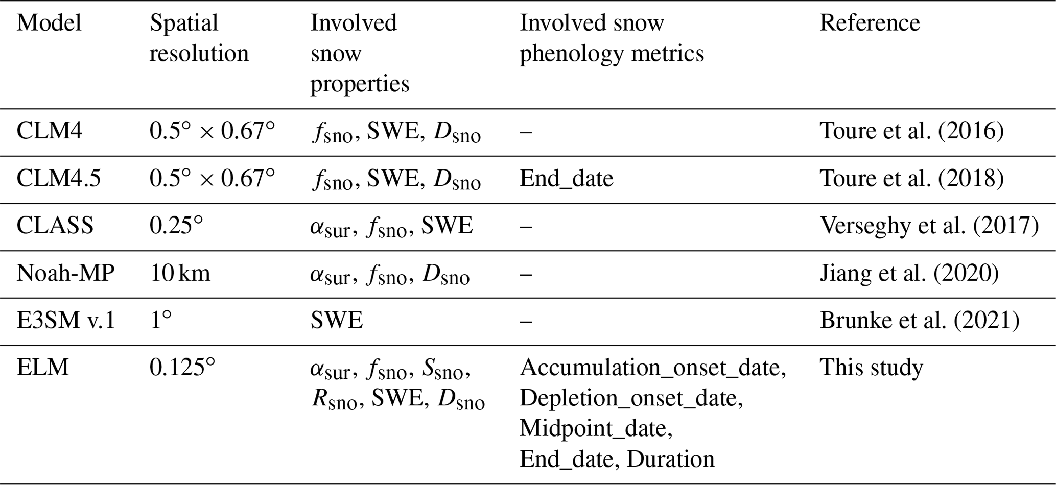
Previous studies evaluated simulations of snow cover fraction (fsno), SWE, snow depth (Dsno) (Toure et al., 2016, 2018), and snowmelt timing (Toure et al., 2018) in the Community Land Model v.4 (CLM4) in the Northern Hemisphere at a coarse spatial resolution of . The 0.25∘ simulations of surface albedo (αsur), fsno, and SWE in the Canadian Land Surface Scheme (CLASS) were evaluated over eastern Canada (Verseghy et al., 2017), but snow phenology was not assessed. Monthly SWE in the 1∘ coupled land–atmosphere simulations of E3SM v.1 was evaluated over the contiguous United States by Brunke et al. (2021), who attributed SWE uncertainties to the biases in temperature and precipitation. Overall, previous studies only evaluated a few snow variables in LSMs mostly at coarse spatial resolutions (Table A2), although more high-resolution remote sensing observations and data assimilation products of snow variables (e.g., snow albedo – αsno, snow grain size – Ssno, and snow albedo reduction induced by LAPs in snow – Rsno) have become available. The snow phenology in LSMs has rarely been evaluated explicitly, and how LSMs capture the interannual variability of snow variables and how those variables vary along an elevation gradient have not been well investigated.
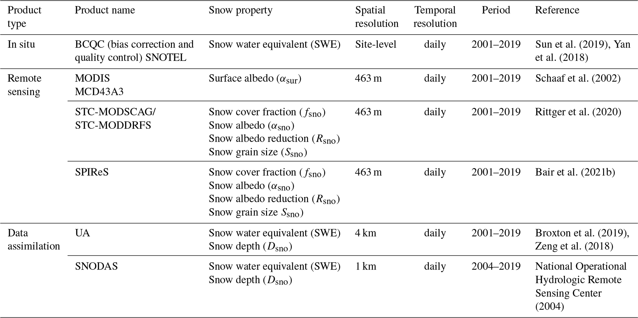
A series of high-quality field snow measurements and remote sensing and data assimilation snow datasets/products with high spatio-temporal resolution are available over the WUS. The in situ Snow Telemetry (SNOTEL) stations widely distributed across the WUS provide long-term SWE field measurements (Serreze et al., 1999). Optical remote sensing data have been widely used to map snow dynamics (Dietz et al., 2012; Dong, 2018). The Moderate Resolution Imaging Spectroradiometer (MODIS) reflectance data at 463 m spatial resolution have been used to retrieve multiple key snow-related variables including αsur (Schaaf et al., 2002), fsno (Bair et al., 2021b; Painter et al., 2009), αsno, Ssno, and Rsno (Bair et al., 2021b; Painter et al., 2012). These MODIS data accurately capture snow dynamics during accumulation and melt (Rittger et al., 2013; Wang et al., 2018), and the high daily temporal resolution of these datasets is helpful for capturing rapid snow variations. Some available remote sensing snow phenology products (Chen et al., 2015; Metsämäki et al., 2018; Takala et al., 2009) adopt different optical or microwave satellite observations to extract snow phenology date and duration. Besides, they use different snow phenology definitions and include different snow phenology metrics, which can affect their use as a reference. Alternatively, the same phenology extraction methods can be used to derive snow phenology metrics for both LSMs and MODIS daily fsno data, avoiding inconsistencies of definitions and extraction methods. Data-assimilated SWE and snow depth (Dsno) products are also available that integrate field measurements, remote sensing observations, and model simulations (National Operational Hydrologic Remote Sensing Center, 2004; Zeng et al., 2018). These data assimilation products have high spatial resolution of <5 km and higher reliability over mountainous and forested regions due to the constraints of in situ networks (Dawson et al., 2018). These datasets provide good opportunity for comprehensively evaluating the accuracy of snow variables and snow phenology in LSMs.
The aim of this study is to systematically evaluate the high-resolution 0.125∘ ELM simulations of key snow variables and snow phenology over the WUS, using in situ, remote sensing, and data assimilation snow products. Specifically, offline ELM simulations with new improvements related to snow processes over the WUS were conducted during 2001–2019. Field snow measurements, three MODIS remote sensing products, and two data assimilation snow products were collected as benchmarking datasets for the ELM simulations (see Sect. 2.3 for details). All the ELM outputs and benchmarking datasets were regridded to an identical spatio-temporal resolution of 0.125∘ and made daily. Snow properties' variables including αsur, fsno, αsno, Ssno, Rsno, SWE, and Dsno were used in the analysis. Multiple snow phenology metrics were derived from both ELM and remote sensing products using the same definitions and extraction methods (see Sect. 2.4 for details). The spatial patterns, temporal correlations, interannual variabilities, elevation gradients, and change with forest cover of snow properties and snow phenology in ELM were evaluated against the benchmarking datasets. Uncertainties in the ELM and benchmarking datasets, implications for model improvements, and limitations of the study are discussed.
2.1 Model description
ELM, the land component of E3SM, originates from the Community Land Model v.4.5 (CLM4.5) (Golaz et al., 2019). ELM uses a multi-layer scheme (up to five layers by default) to dynamically simulate various snow processes, e.g., snow accumulation, melting, aging (i.e., the evolution of snow grain size), compaction, metamorphism, aerosol deposition and redistribution, and canopy snow interception and unloading. Specifically, ELM uses the snow, ice, and aerosol radiative (SNICAR) model to calculate snow albedo and vertically-resolved absorption of solar radiation, considering the evolving snow grain size, solar zenith angles (SZAs), sky conditions, underlying background, and snow impurities (e.g., black carbon, BC, and dust) (Flanner et al., 2007). ELM uses the snow water equivalent (SWE) and standard deviation of elevation to estimate snow cover fraction (fsno). The hysteresis of snow accumulation and ablation is also accounted for in ELM (Swenson and Lawrence, 2012).
Compared to CLM4.5, some key updates related to snow processes have been included in ELM. First, the original SNICAR model has been replaced by a hybrid model (SNICAR-AD) of SNICAR and delta-Eddington adding–doubling radiative transfer solver, which corrects the snow albedo bias for large SZAs and can better represent the shortwave radiative properties of snow (Dang et al., 2019). Second, compared to only external mixing in CLM4.5, both external mixing and internal mixing of hydrophilic BC snow and dust snow are now represented in ELM (Hao et al., 2023; Wang et al., 2020). Third, the direct and diffuse irradiance under different atmospheric profiles and their dependence on SZA are included (Hao et al., 2023). Fourth, the effects of non-spherical snow grain shape on snow albedo are considered (Hao et al., 2023). Fifth, a new parameterization of subgrid topographic effects on solar radiation has been implemented in ELM to account for the impacts of macroscale shadow, occlusion, and multi-scattering between adjacent terrain on surface albedo (Hao et al., 2021, 2022).
2.2 Model setup and experiment design
Selected for this study, the WUS has heterogeneous topography with diverse elevations ranging from 0 to above 3 km (Fig. 1a). The WUS includes three major mountain ranges: the Cascades Range, Sierra Nevada, and Rocky Mountains, which are characterized by frequent snow cover. The elevation data were acquired from the Shuttle Radar Topography Mission (SRTM) DEM dataset (Rabus et al., 2003). The forest cover data in 2010 shown in Fig. 1b were acquired from the 30 m Landsat Vegetation Continuous Fields (VCF) tree cover datasets derived from the Global Forest Cover Change (GFCC) surface reflectance product (Sexton et al., 2013). Both the DEM and forest cover data were aggregated to 0.125∘ using the area-weighted average method. For analysis, elevations were divided into different intervals (see Fig. 1c). Elevations less than 0.5 km are not included in the statistical analysis, as snow cover is close to 0. The forest cover was divided into five levels (see Fig. 1d). The area fractions of different intervals of elevation and forest cover are shown in Fig. 1c and d, respectively.
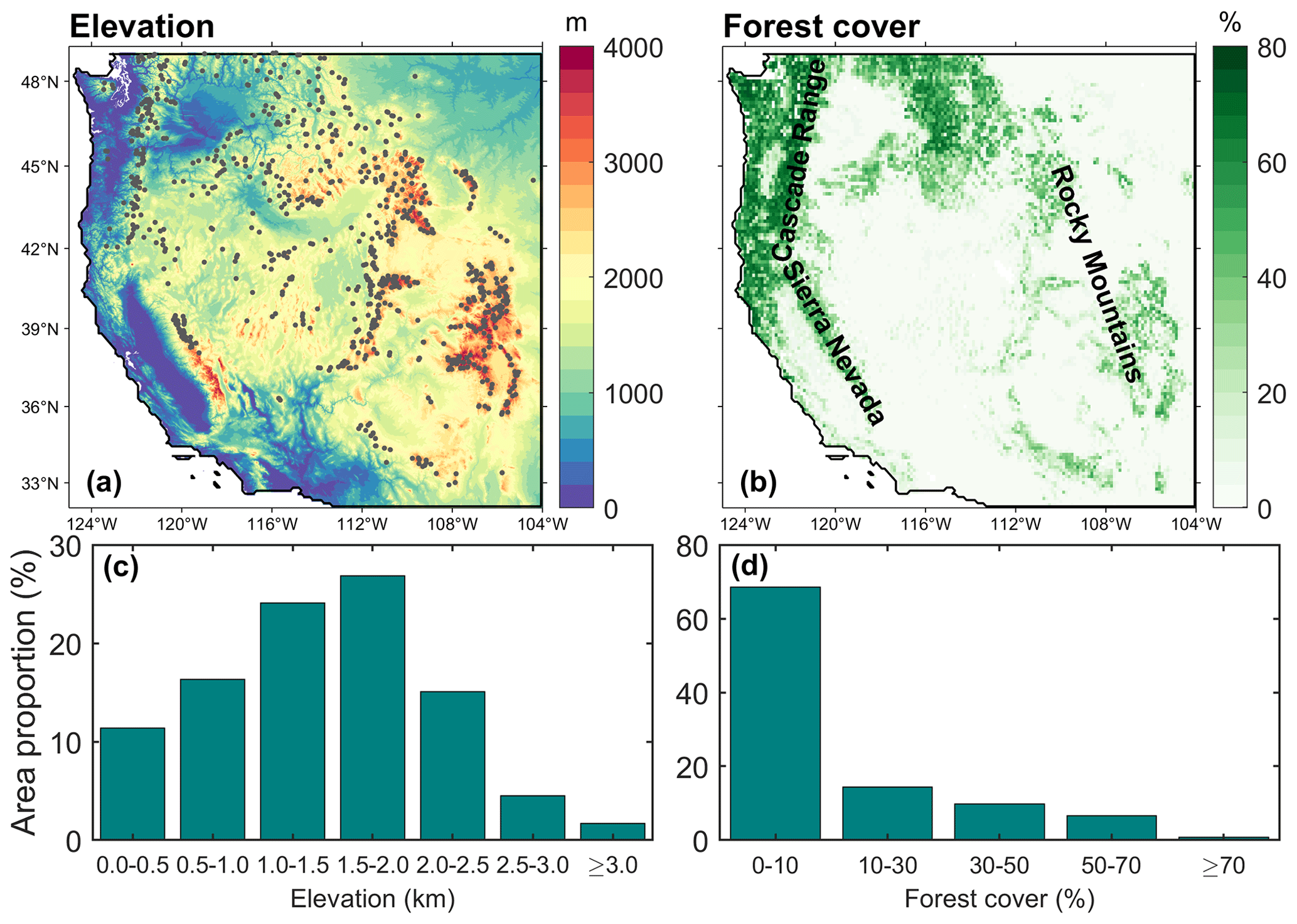
Figure 1Spatial distributions of (a) elevation and SNOTEL sites (grey points) and (b) forest cover over the WUS, and the area proportions of different (c) elevation and (d) forest cover intervals. The Cascades Range, Sierra Nevada, and Rocky Mountains are highlighted in panel (b).
ELM simulations at 0.125∘ spatial resolution were conducted over the WUS from 1979 to 2019 driven by hourly meteorological forcing data from the National Land Data Assimilation System phase 2 (NLDAS-2) with spatial resolution of 0.125∘ (Xia et al., 2012). Specifically, the prescribed satellite phenology (SP) mode was used with input of MODIS leaf area index data (Myneni et al., 2002). The climatological monthly aerosol deposition data (e.g., black carbon and dust) with a spatial resolution of from the Community Atmosphere Model v.5 coupled with chemistry (Lamarque et al., 2010) were used, which were temporally and spatially downscaled to half-hourly and 0.125∘ using bilinear interpolation. For the snow albedo module, SNICAR-AD was configured with: (1) the SZA-dependence solar irradiance under the mid-latitude winter atmosphere, (2) spherical snow grain shape, (3) internal mixing of hydrophilic BC snow, (4) external mixing of dust snow, and (5) neglect of organic carbon due to its high uncertainties. The subgrid topographic effects on solar radiation were included in the ELM configuration. The model was run at a half-hourly step. The first 31-year run from 1979 to 2000 was used to spin up the model to reach equilibrium, and then the remaining 19-year run (i.e., 2001–2019) was used in the analysis. The variables of interest were output at half-hourly, daily, and monthly scales.
Table 1Summary of the in situ, remote sensing, and data assimilation datasets used in the study. These datasets provide different snow properties' variables, and snow cover fraction in both STC-MODSCAG/STC-MODDRFS and SPIReS was used to derive snow phenology metrics.
2.3 Benchmarking datasets
In situ bias correction and quality control (BCQC) SNOTEL daily SWE data from 2001–2019 (Table 1) were used as the benchmarking dataset to evaluate the performance of ELM. SNOTEL stations, operated by the US Department of Agriculture Natural Resources Conservation Service (NRCS), provide long-term, widely-distributed, and high-quality field measurements of SWE across the WUS (https://www.nrcs.usda.gov/, last access: 4 February 2023). BCQC SNOTEL eliminated data outliers and erroneous values, fixed the inconsistencies of different variables, and corrected the bias of the raw data (Sun et al., 2019; Yan et al., 2018). Specifically, 788 SNOTEL sites in the WUS were included in the study (Fig. 1a).
Three daily 463 m MODIS-based remote sensing products from 2001–2019 were used to evaluate the performance of ELM (Table 1). The first one is the MCD43A3 surface albedo v.6 product (named as MCD43 hereafter). The MCD43 product provides black-sky and white-sky surface albedo at local solar noon (Schaaf et al., 2002), which could well capture the snow effects on αsur (Wang et al., 2018). This dataset represents the albedo of the entire MODIS pixel which could include vegetation or soil if the observed pixel is not 100 % snow cover, and thus it will underestimate snow albedo for fractionally covered pixels, as vegetation and soil have darker broadband albedos. The second one is the spatially and temporally complete (STC) MODIS snow-covered area and grain size (MODSCAG) and MODIS dust and radiative forcing in snow (MODDRFS) product (hereafter referred to as STC-MODSCAG/STC-MODDFRS). The third one is the snow property inversion from remote sensing (SPIReS) product. These two products provide fsno, αsno, Ssno, and Rsno at around 10:30 LST (local solar time) and represent αsno (i.e., excluding soil and vegetation portions of the observed pixel). STC-MODSCAG first estimates fsno and Ssno based on the spectral unmixing and physically-based snow radiative transfer models (Painter et al., 2009). STC-MODDRFS then uses Ssno to calculate the αsno of the clean snow with the difference between clean and dirty (observed) snow for computing Rsno (Painter et al., 2012). SPIReS adopts a physically-based approach without empirical assumptions to simultaneously estimate fsno, αsno, Ssno, and Rsno (Bair et al., 2021b). Both STC-MODSCAG/STC-MODDRFS and SPIReS are interpolated and smoothed to reduce the effects of data noise, cloud contamination, and sun-sensor geometry (Bair et al., 2021b; Dozier et al., 2008; Rittger et al., 2020). Both of the fsno products show good performance with the basin-wide root mean square error (RMSE) values of 6.5 % and 6.7 % against airborne lidar datasets (Stillinger et al., 2022). Initial validation against field measurements for Ssno at a single site for the original MODSCAG shows a 51 µm mean absolute error for a clear sky day (Painter et al., 2009). The gap-filled MODSCAG/MODDRFS at three sites in the WUS has an accuracy (RMSE) of 118 µm for Ssno and 0.0036 for Rsno (Bair et al., 2019) considering both clear and cloud days. SPIReS has a αsno RMSE of 4.6 % against the 3-year field measurements at Mammoth Mountain, CA (Bair et al., 2021b), nearly identical to the reported accuracy of 4.8 % RMSE for STC-MODDRFS against the field measurements at the same site (Bair et al., 2019). Note that there is an underestimation of fsno in the northern WUS region in winter occurring because of a known issue in current versions of STC-MODSCAG (https://nsidc.org/snow-today, last access: 4 February 2023). Specifically, MOD09GA surface reflectance processed to produce STC-MODSCAG at the Jet Propulsion Laboratory (JPL) is not processed when SZA is larger than 67.5∘. This issue is being resolved during the transfer of processing during 2022 to 2023 from JPL to the National Snow and Ice Data Center Distributed Active Archive. We conservatively excluded data north of 42∘ in latitude during the winter in our comparisons in Sect. 3.1.
Two data assimilation SWE and Dsno products from 2001–2019 were used to compare with ELM (Table 1). The first one is the University of Arizona (UA) daily snow product v.1 with the spatial resolution of 4 km over the conterminous US (Zeng et al., 2018). This product was generated by fully utilizing the field measurements from multiple in situ networks, including SNOTEL constrained by the gridded precipitation and temperature data in the 4 km parameter-elevation regressions on independent slopes model (PRISM). A series of algorithm robustness tests and independent accuracy evaluations against remote sensing and airborne lidar measurements showed that the UA product is reliable as a reference snowpack dataset (Zeng et al., 2018). The second one is the SNOw Data Assimilation System (SNODAS) daily product with 1 km spatial resolution developed by the NOAA National Weather Service's National Operational Hydrologic Remote Sensing Center (National Operational Hydrologic Remote Sensing Center, 2004). SNODAS uses a physically consistent modeling and data assimilation framework to integrate physically-based model estimates and multi-source snow data from satellite remote sensing, airborne-based observations, and in situ measurements including SNOTEL. SNODAS has shown a similar performance as UA (Zeng et al., 2018). The SNODAS product is available from October 2003, and thus only the data from 2004–2019 were used in the study. UA and SNODAS both assimilate the SNOTEL observations in their models directly, so better performance relative to those observations is expected, while the ELM simulations are not constrained by the SNOTEL data.
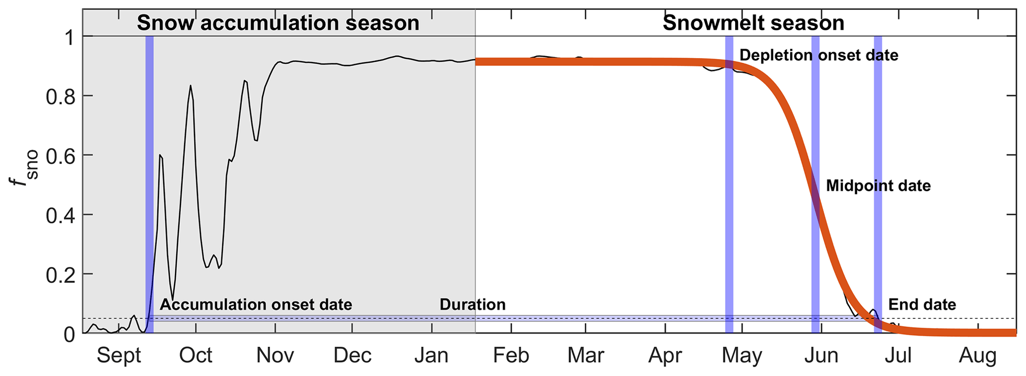
Figure 2Time series of snow cover fraction (fsno) and sigmoid curve fitting at a typical pixel, represented by black and red lines, respectively. The blue lines indicate four phenology dates and one duration, and the shaded area shows the snow accumulation season.
2.4 Snow phenology extraction and data processing
Time series of fsno from ELM and two remote sensing snow products (i.e., STC-MODSCAG and SPIReS) were used to extract the snow phenology (Fig. 2). First, based on the observed seasonal cycle of snow cover over the WUS (Brutel-Vuilmet et al., 2013; Peng et al., 2013; Rittger et al., 2022), the snow accumulation and snowmelt seasons are defined as the periods from September to January and from February to August, respectively. Next, four snow timing dates and one duration metric were retrieved from ELM and remote sensing products that include: (1) snow accumulation onset date (Accumulation_onset_date), (2) snow cover depletion onset date (Depletion_onset_date), (3) snow cover depletion midpoint date (Midpoint_date), (4) snow end date (End_date), and (5) snow duration days (Duration). Following Peng et al. (2013), Accumulation_onset_date for year t is defined as the first continuous 5 d with fsno>0.05 during the snow accumulation season from September (year t−1) to January (year t), and End_date is defined as the last continuous 5 d with fsno>0.05 during the snowmelt season of the year t, to avoid the interference of ephemeral snow. Note that using different thresholds (e.g., 0.00, 0.03, 0.05, 0.10, 0.15) of fsno to defining Accumulation_onset_date and End_date can lead to different date estimates but the same conclusions, which are not shown in the paper. Duration was calculated as the number of days between Accumulation_onset date and End_date. Depletion_onset_date and Midpoint_date were determined by fitting the fsno time series during the snowmelt season using the sigmoid function (Anttila et al., 2018; Böttcher et al., 2014; Kouki et al., 2019) as follows:
where DOY is day of year, and a, b, c, and d are the fitted parameters. Specifically, the nonlinear least squares method was used to fit a sigmoid function. Following Anttila et al. (2018), Depletion_onset_date is defined as the date when the fitted sigmoid curve reaches 99 % of its variation range, and Depletion_midpoint_date is defined as the date at the midpoint of the curve change (Fig. 2). To reduce the impacts of noise, the retrievals at the individual pixels for a specific year was deemed as unsuccessful when: (1) the fsno difference at the start and end date of snowmelt season is smaller than 0.05; and (2) for the sigmoid fitting, the coefficient of determination (R2) between observed and fitted fsno is smaller than 0.95 and RMSE is larger than 0.2. Only the pixels with successful retrievals of snow timing metrics for at least 10 years were used in the subsequent analysis.
MODIS data and ELM outputs were adjusted for temporal consistency and to unify the variable definitions. MCD43 only provides black-sky and white-sky albedo, and thus the ELM-derived ratio of diffuse to total solar radiation was used as a weighting factor to calculate αsur for the blue sky. For ELM, the average values of αsur from 11:30 to 00:30 LST were calculated to match the time of MODIS MCD43 product, and those of fsno, αsno, Ssno, and Rsno from 10:00 to 11:00 LST were calculated for ELM to match the time of STC-MODSCAG/STC-MODDRFS and SPIReS.
The snow timing metrics and snow variables in the remote sensing and data assimilation products (Table 1) were aggregated to 0.125∘ using the area-weighted average method. They were temporally upscaled to seasonal, annual, and multi-year average scales. For a specific year, only the pixels with fsno>0 were used to calculate the regional average values for αsur, fsno, αsno, Ssno, Rsno, SWE and Dsno using the area-weighted average method.
2.5 Evaluation methods
Using the field measurements, remote sensing products, and data assimilation products as the reference, the spatio-temporal distributions of ELM snow outputs were evaluated. For spatial correlation, multiple statistical metrics were calculated for the multi-year average seasonal ELM outputs: correlation coefficient (R), bias, relative bias (rBias, calculated as the ratio of bias to the average value), root mean square deviations (RMSDs), and relative RMSD (rRMSD, calculated as the ratio of RMSD to the average value). This study mainly focused on winter (DJF) and spring (MAM) in the analysis, and there is little or no snow cover for the WUS in Summer (JJA) and Autumn (SON) in the ELM simulations (Fig. S1 in the Supplement). For the temporal correlation, R between ELM and the reference datasets was calculated only for the grids where there are at least 10 snow-covered days for 1 year, excluding highly ephemeral snow.
The long-term trends of snow variables over the whole WUS were detected using the non-parametric Mann–Kendall (MK) test. However, the MK test showed that there is no significant increasing or decreasing trend (p-value > 0.05) for all the snow variables, and thus the corresponding results are not included in the paper. The interannual variabilities (IAVs), defined as the standard deviation of the annual values, were calculated to evaluate whether ELM can capture the interannual variations of snow processes. In addition, the distributions of snow variables along the elevation gradients and forest cover for winter and spring were also analyzed.
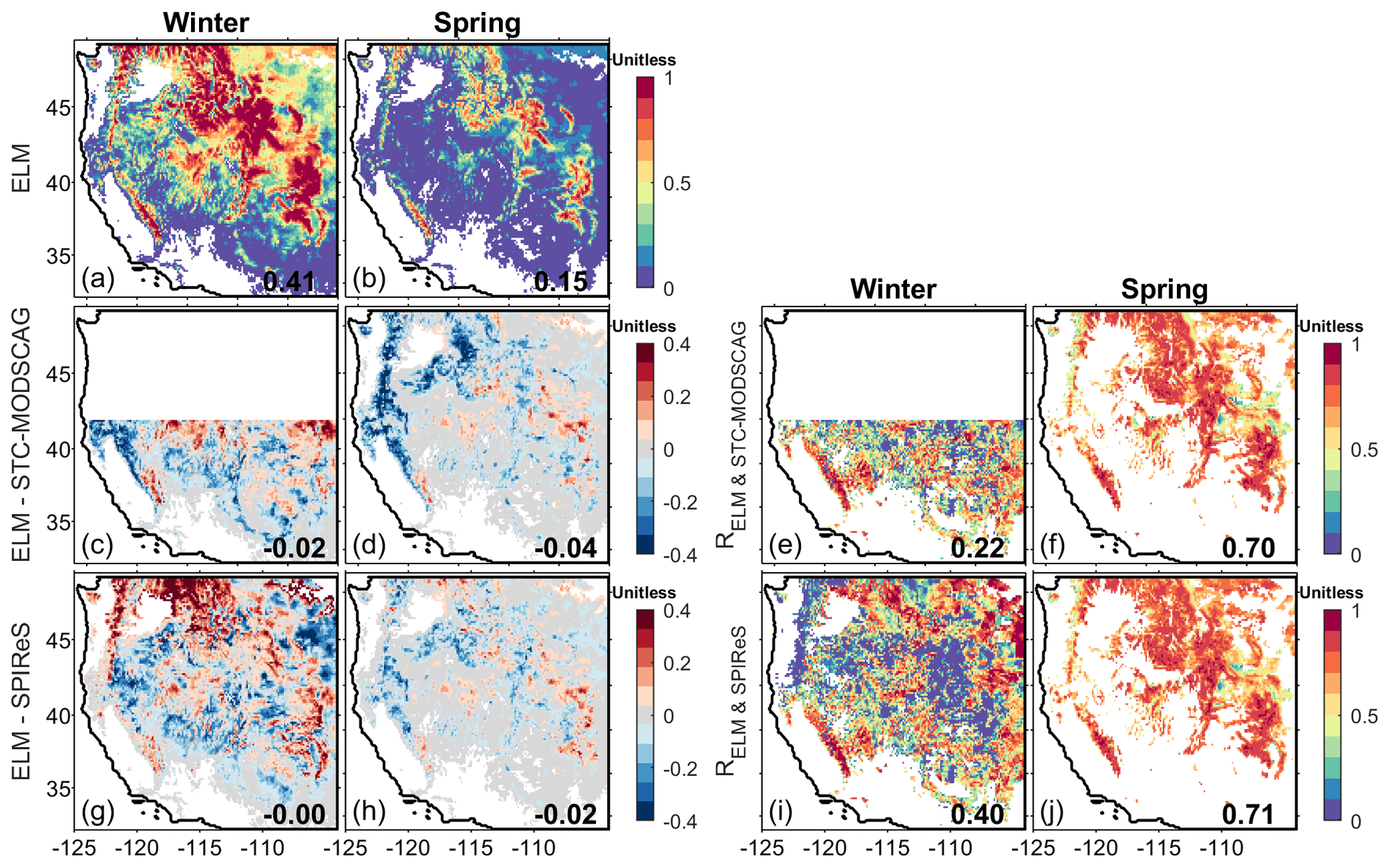
Figure 3Spatial distributions of (a, b) snow cover fraction (fsno) in ELM, and (c, d, g, h) the fsno difference between ELM and two remote sensing products (i.e., STC-MODSCAG and SPIReS) and (e, f, i, j) their temporal correlations (Rs) for different seasons: (a, c, e, g, i) winter and (b, d, f, h, j) spring. In all panels, regions with no snow cover are masked with white color. The area-weighted average values are labeled in each panel.
3.1 Snow properties
3.1.1 Snow cover fraction
The ELM-simulated fsno has heterogeneous spatial patterns in the WUS for both winter and spring (Fig. 3a and b). The regional average fsno is 0.41 and 0.15, respectively, for winter and spring. Overall, ELM also shows similar spatial patterns with both STC-MODSCAG and SPIReS for all the seasons (Fig. S1). STC-MODSCAG underestimates fsno over the northern regions in winter due to the known issues (Fig. S1, see Sect. 2.3 for details). When excluding December and January with larger SZAs, STC-MODSCAG shows similar spatial distribution as SPIReS for February (Fig. S2). In spring, compared to STC-MODSCAG, ELM underestimates fsno over the western mountains in spring (Fig. 3d). Compared to SPIReS, ELM has an overestimation over most regions in winter but performs well in spring (Fig. 3g and h). Overall ELM has a high spatial correlation to both STC-MODSCAG and SPIReS, with a higher relative accuracy in winter than spring (Table 2). For temporal correlation, ELM has a low correlation in the mountainous areas with both STC-MODSCAG and SPIReS in winter (Fig. 3e and i) but has a relatively high correlation with those data in spring (Fig. 3f and j). The winter–spring contrast in skill is possibly due to the smaller change of fsno in winter than spring.
Table 2Evaluation of snow properties in ELM against two remote sensing products (STC-MODSCAG/STC-MODDRFS and SPIReS) and two data assimilation products (UA and SNODAS) for winter and spring. Here, the snow properties include snow cover fraction (fsno), surface albedo (αsur), snow albedo (αsno), snow grain size (Ssno), snow albedo reduction (Rsno), snow water equivalent (SWE), and snow depth (Dsno). The statistical metrics were calculated using the data over the WUS, except that those against STC-MODSCAG/STC-MODDRFS in winter were calculated using the data over the WUS regions below 42∘ in latitude.

ELM well reproduces the interannual variabilities and elevation gradients of fsno (Figs. 4 and S3). The IAV values are 0.055 and 0.049, respectively, for ELM and SPIReS in winter, while they have closer values of 0.027, 0.029, and 0.030, respectively, for ELM, STC-MODSCAG, and SPIReS in spring (Fig. 4a and b). ELM underestimates regional average fsno in spring and is overall consistent with STC-MODSCAG and SPIReS in terms of magnitude and IAVs. As the elevation increases, fsno values in all three datasets become higher for both winter and spring (Fig. 4c and d). At relatively low elevation, the fsno distributions in ELM are broader than those of SPIReS in winter, while the three datasets have more consistent elevation gradients in spring. Overall, when forest cover is higher, ELM shows larger differences with SPIReS for spring and STC-MODSCAG for winter (Fig. 4e and f). Same conclusions can be drawn for the regions below 42∘ in latitude (Fig. S3). Considering the uncertainties of the remote sensing retrievals, the ELM regional average fsno is within the range of STC-MODSCAG and SPIReS (Figs. 5a, b, and S4).
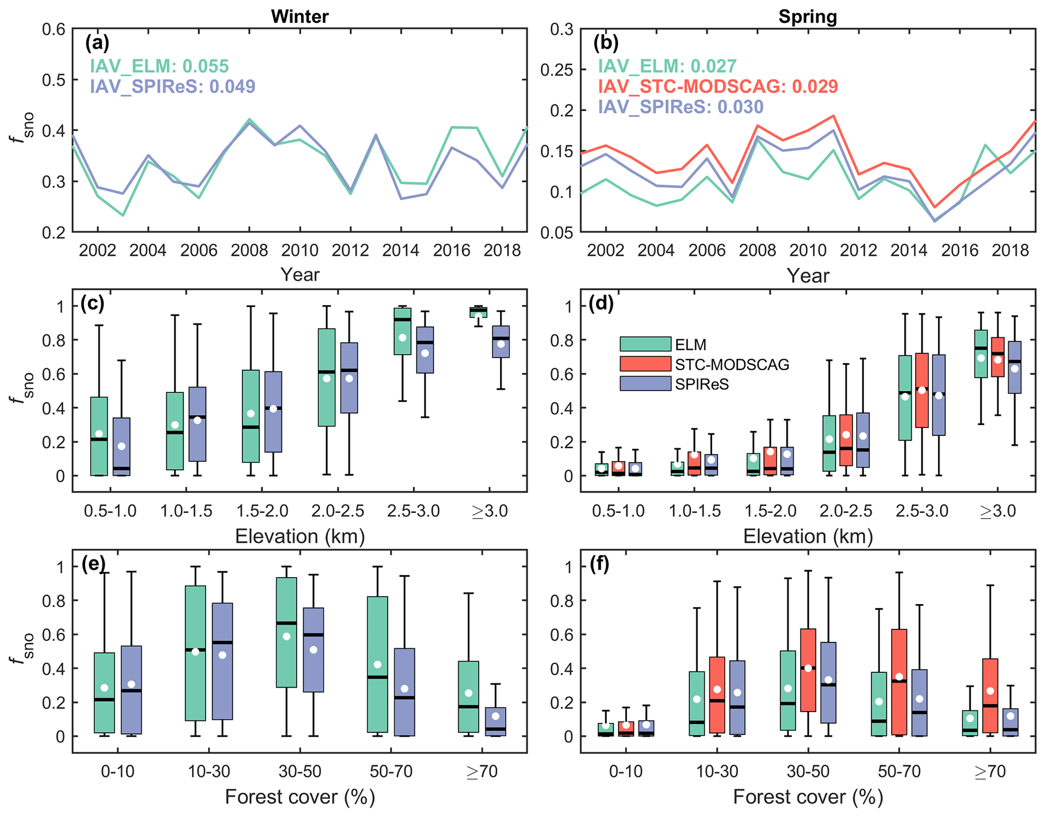
Figure 4(a, b) Time series of regional average values, (c, d) elevation gradients, and (e, f) change with forest cover of snow cover fraction (fsno) in ELM (green), STC-MODSCAG (red), and SPIReS (blue) over the WUS. Panels (a, c, e) are for winter, and panels (b, d, f) are for spring. In panels (c–f), the white dots represent the average values.

Figure 5The area-weighted average (a, b) snow cover fraction (fsno), (c, d) snow grain size (Ssno), and (e, f) snow albedo reduction (Rsno) for (a, c, e) winter and (b, d, f) spring of ELM (green), STC-MODSCAG/STC-MODDRFS (red), and SPIReS (blue) over the WUS. The bar width represents the uncertainty bounds of STC-MODSCAG/STC-MODDRFS and SPIReS from Bair et al. (2021a).
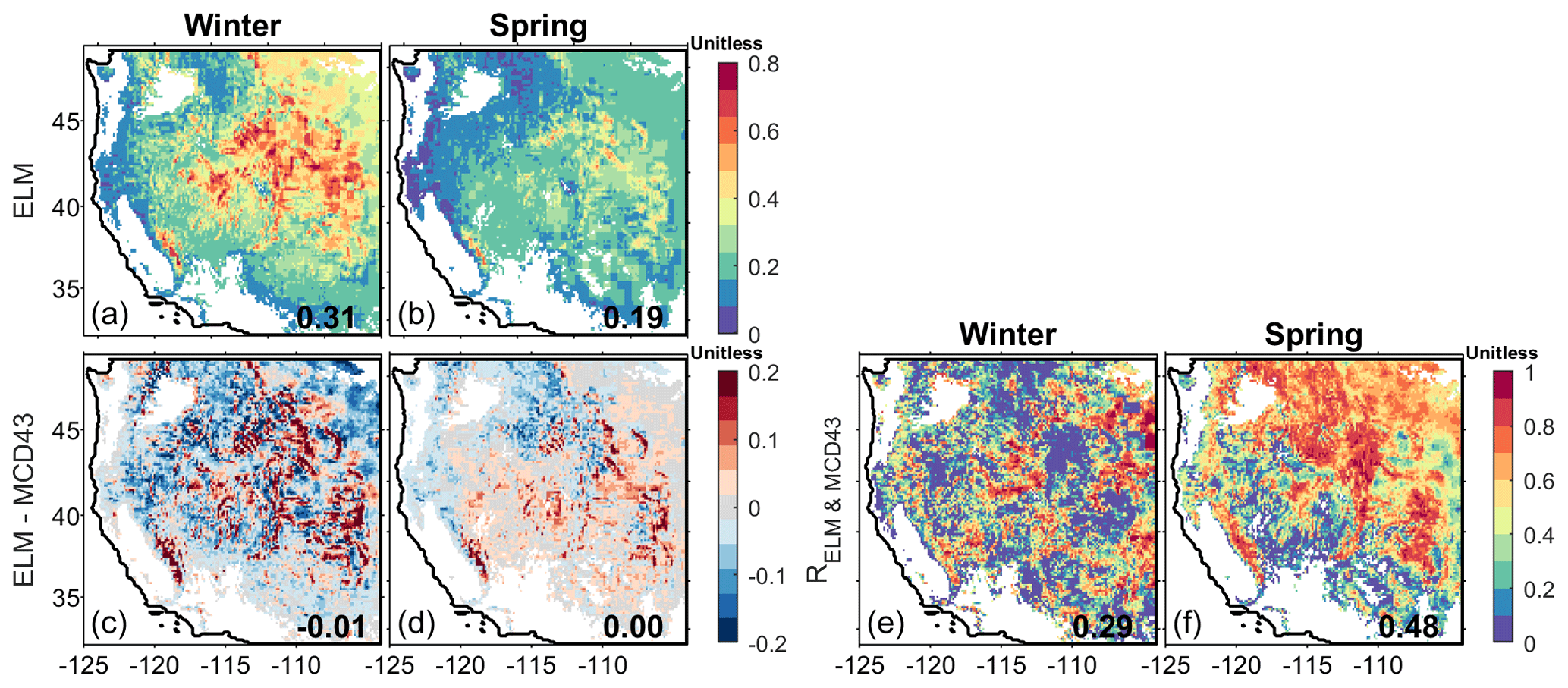
Figure 6Spatial distributions of (a, b) surface albedo (αsur) in ELM, and (c, d) the αsur difference between ELM and MCD43 and (e, f) their temporal correlations (Rs) for different seasons: (a, c, e) winter and (b, d, f) spring. In all panels, the regions with no snow cover are masked with white color. The area-weighted average values are labeled in each figure.

Figure 7(a, b) Time series of regional average values, (c, d) elevation gradients, (e, f) change with forest cover, and (g, h) statistical distributions of surface albedo (αsur) under different snow cover conditions in ELM (green) and MCD43 (red) for different seasons: (a, c, e, g) winter and (b, d, f, h) spring over the WUS. The IAV values of different datasets are shown in (a, b). In panels (c)–(h), the white dots represent the average values.
3.1.2 Surface albedo and snow albedo
Overall, the ELM-simulated αsur over snow cover regions shows similar spatio-temporal distribution with MCD43 for both winter and spring (Figs. 6 and 7). Compared to MCD43, ELM overestimates αsur over Sierra Nevada and Rocky Mountains in winter, possibly due to the bias in snow cover (Fig. 3c and d). The mean biases of ELM are −0.01 and 0.00, respectively, for winter and spring. The spatial R values between ELM and MCD43 are 0.77 and 0.71, respectively, for winter and spring (Table 2). ELM shows a low temporal correlation to MCD43 over most regions in winter but has a relatively higher temporal correlation in spring especially over the mountain areas and northern regions (Fig. 6e and f). ELM also has similar interannual variability especially in winter (Fig. 7a and b), similar elevation gradient (Fig. 7c and d), and similar distributions under different forest cover (Fig. 7e and f) with MCD43. As fsno increases, αsur in both ELM and MCD43 increases, and ELM and MCD43 have similar αsur distributions for different elevation intervals (Fig. 7g and h).
For αsno, ELM overall shows good consistencies with STC-MODDRFS and SPIReS over mountainous regions but has an underestimation over other regions (Fig. 8). Against STC-MODDRFS, the mean biases of ELM are −0.08 for winter over the WUS regions below 42∘ in latitude and −0.11 for spring over the WUS. Against SPIReS, the mean biases of ELM are −0.13 and −0.08, respectively, for winter and spring. The spatial R values between ELM and two remote sensing products are lower than 0.30 (Table 2). ELM shows a low temporal correlation to two remote sensing products over most regions and has a relatively higher temporal correlation over the Rocky Mountains (Fig. 8e and f). Larger inconsistencies between ELM and two remote sensing products are founded in terms of interannual variations, elevation gradients, and change with forest cover (Figs. 9 and S5).
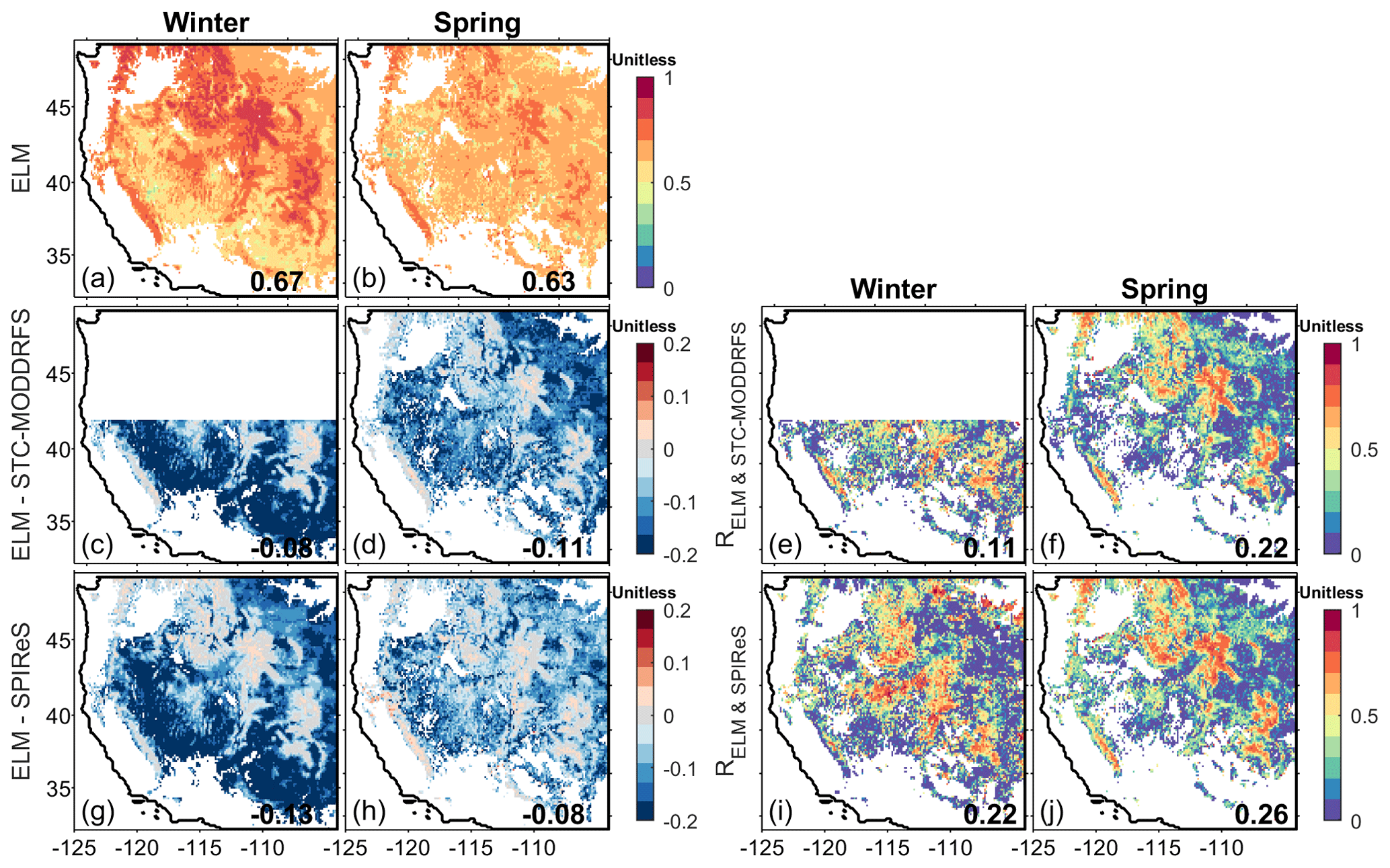
Figure 8Spatial distributions of (a, b) snow albedo (αsno) in ELM, and (c, d, g, h) the αsno difference between ELM and two remote sensing products (i.e., STC-MODDRFS and SPIReS) and (e, f, i, j) their temporal correlations (Rs) for different seasons: (a, c, e, g, i) winter and (b, d, f, h, j) spring. In all panels, regions with no snow cover are masked with white color. The area-weighted average values are labeled in each panel.
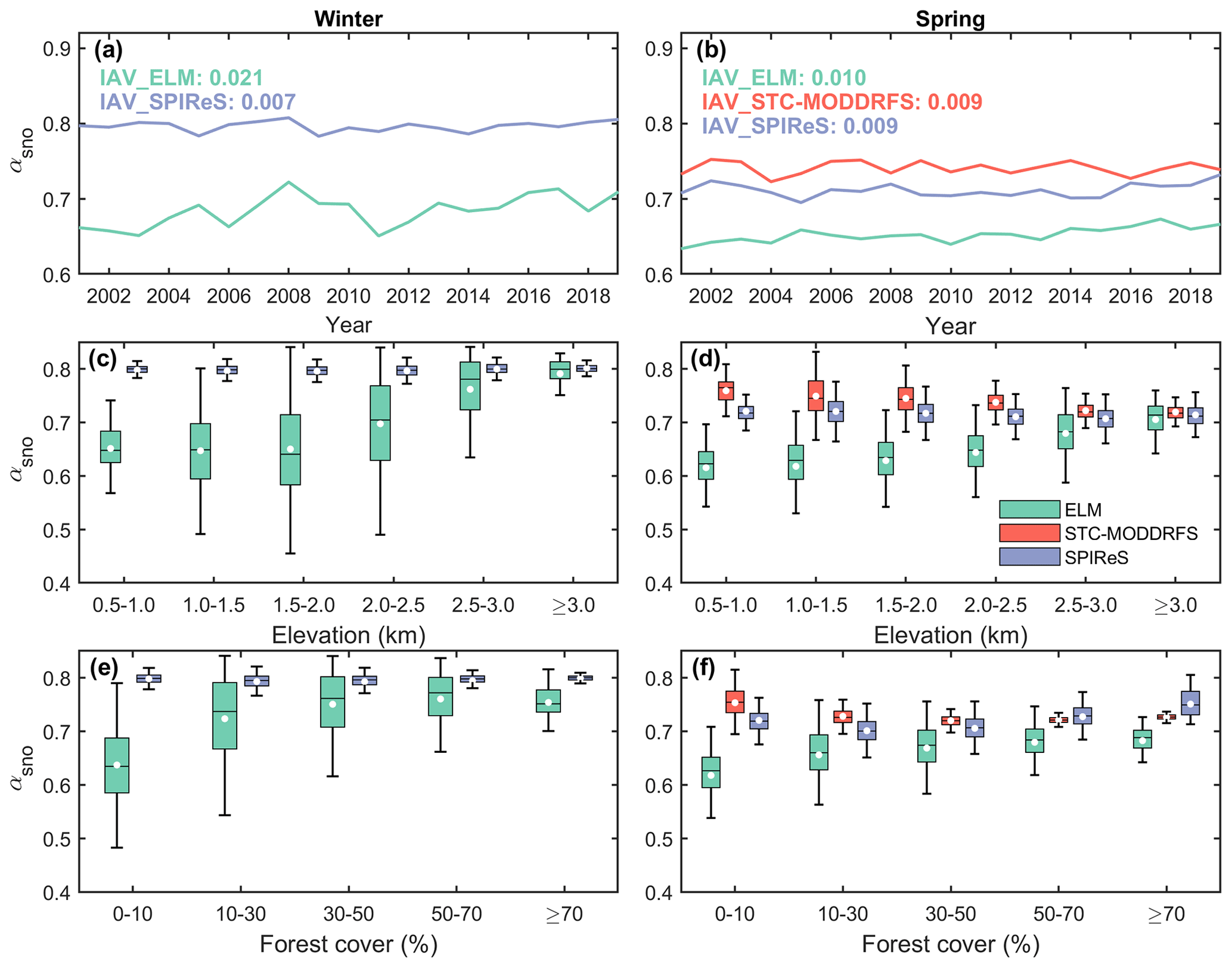
Figure 9(a, b) Time series of regional average values, (c, d) elevation gradients, and (e, f) change with forest cover of snow albedo (αsno) in ELM (green), STC-MODSCAG (red), and SPIReS (blue) over the WUS. Panels (a, c, e) are for winter, and panels (b, d, f) are for spring. In panels (c)–(f), the white dots represent the average values.
3.1.3 Snow grain size and snow albedo reduction
There are large differences in the magnitudes and spatio-temporal patterns of Ssno between ELM and STC-MODSCAG/SPIReS (Figs. 10 and 11). ELM has larger Ssno in spring than in winter (Fig. 10a and b), with large negative biases over the western mountains and positive biases over the central and eastern regions compared to STC-MODSCAG, with the mean biases of −71.6 µm for spring (Fig. 10c and d). ELM has positive biases over most regions compared to SPIReS, with the mean bias of 93.9 and 31.6 µm for winter and spring, respectively (Fig. 10g and h). Ssno in ELM has a poor spatial correlation to the two MODIS products for both winter and spring (Table 2). ELM has varying temporal correlations with STC-MODSCAG and SPIReS for both seasons with a mean value of around 0.3 (Fig. 10e, f, i, and j). ELM has a similar interannual variability to SPIReS (Figs. S6a, b and S7a, b). As the elevation increases, ELM and SPIReS have decreasing Ssno in winter, but there is no obvious and comparable pattern along the elevation in spring (Figs. S6c, d and S7c, d). As forest cover increases, the three data show larger differences for spring (Figs. S6f and S7f). Considering the uncertainties of Ssno in the remote sensing products, the regional average Ssno is within the range between STC-MODSCAG and SPIReS (Figs. 5c, d and S4).

Figure 10Spatial distributions of (a, b) snow grain size (Ssno) in ELM, and (c, d, g, h) the Ssno difference between ELM and two remote sensing products (i.e., STC-MODSCAG and SPIReS) and (e, f, i, j) their temporal correlations (Rs) for different seasons: (a, c, e, g, i) winter and (b, d, f, h, j) spring. In all panels, regions with no snow cover are masked with white color. The area-weighted average values are labeled in each panel.

Figure 11Spatial distributions of (a, b) snow albedo reduction (Rsno) in ELM, and (c, d, g, h) the Rsno difference between ELM and two remote sensing products (i.e., STC-MODDRFS and SPIReS) and (e, f, i, j) their temporal correlations (Rs) for different seasons: (a, c, e, g, i) winter and (b, d, f, h, j) spring. In all panels, regions with no snow cover are masked with white color. The area-weighted average values are labeled in each panel.
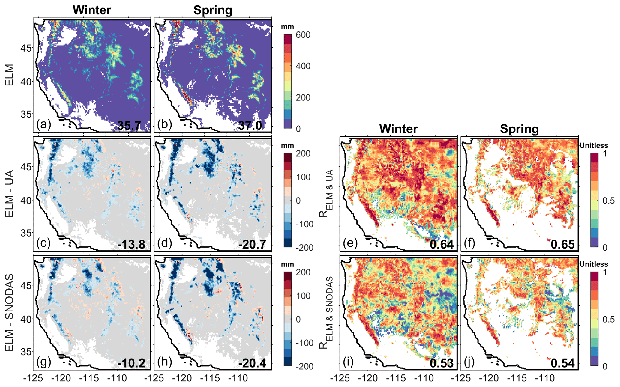
Figure 12Spatial distributions of (a, b) snow water equivalent (SWE) in ELM, and (c, d, g, h) the SWE difference between ELM and two data assimilation products (i.e., UA and SNODAS) and (e, f, i, j) their temporal correlations (Rs) for different seasons: (a, c, e, g, i) winter and (b, d, f, h, j) spring. In all panels, regions with no snow cover are masked with white color. The area-weighted average values are labeled in each panel.
There are also large spatial biases and low temporal correlations of Rsno between ELM, STC-MODDRFS, and SPIReS (Figs. 11 and S4). In ELM, Rsno shows extremely high values in the northeastern corner for winter (Fig. 11a), due to the large aerosol deposition in the aerosol deposition data (see Sect. 2.2). Apart from the northeastern corner, ELM is more similar to SPIReS in winter (Fig. 11c–g). For spring, ELM is more similar to STC-MODSCAG and has large negative biases relative to SPIReS (Fig. 11d–h). ELM has higher temporal correlations with both remote sensing products in winter than spring and shows higher correlations with SPIReS than STC-MODDRFS in spring (Fig. 11e, f, i and j). For interannual variability, ELM is more identical to STC-MODSCAG in spring (Figs. S8a, b and S9a, b) than SPIRES. However, note that ELM simulations in the study used climatological monthly aerosol deposition data, so they are not comparable to the remote sensing data in any specific year. In spring, Rsno in all the three datasets shows an increasing trend with elevation (Figs. S8d and S9d). All the three data show larger differences across different forest cover (Figs. S8e, f and S9e, f). Overall, Rsno is within the uncertainty ranges of STC-MODSCAG and SPIReS (Figs. 5e, f and S4).
3.1.4 Snow water equivalent and snow depth
ELM shows higher SWE values over the mountainous areas (Fig. 12a and b) but also has larger underestimations over the mountainous areas, compared to both UA and SNODAS in both winter and spring (Fig. 12c, d, g and h). Against UA and SNODAS, ELM has a mean bias of −20.7 mm (35.9 %) and −20.4 mm (−35.5 %), respectively, in spring, while those in winter are −13.8 mm (−27.8 %) and −10.2 mm (−22.2 %), respectively. Overall ELM has a high spatial similarity with both UA and SNODAS, and ELM has higher spatial consistency with UA than SNODAS in spring (Table 2). For temporal correlation (Fig. 12e, f, i, and j), ELM has high mean R values of 0.64 and 0.65 for winter and spring, compared to UA, and the R values are 0.53 and 0.54, respectively, compared to SNODAS. ELM captures the interannual variabilities and elevation gradients of SWE well, but some underestimations of the regional average values are observed (Fig. 13a–d). In winter, ELM has similar IAV values to UA and SNODAS but has a lower value of 11.7 mm compared to UA (16.7 mm) and SNODAS (18.1 mm) in spring. Overall, ELM shows larger differences from UA and SNODAS when there is a higher forest cover, especially for spring (Fig. 13e and f). Dsno shows very similar results to SWE (Figs. S10 and S11).
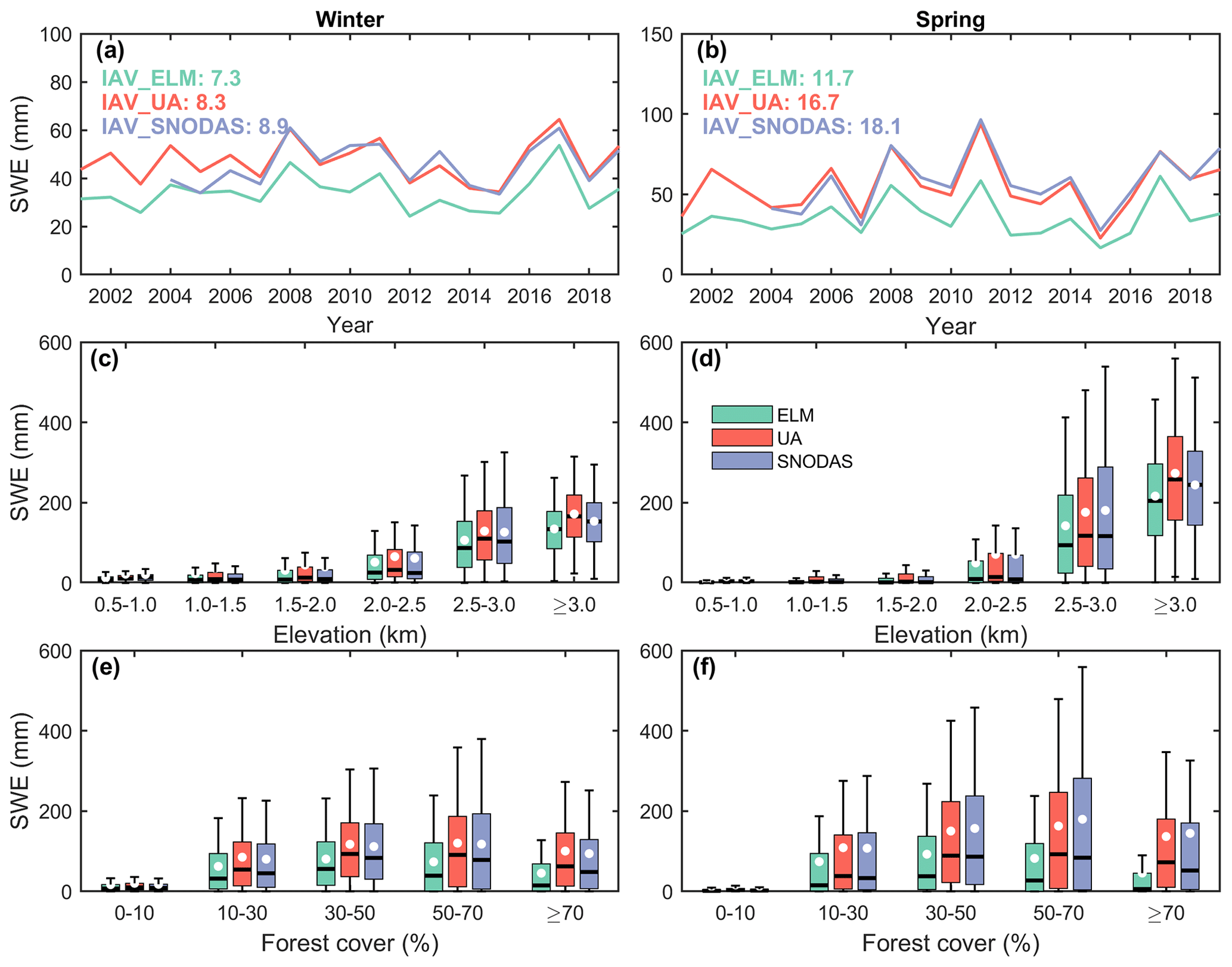
Figure 13(a, b) Time series of regional average values, (c, d) elevation gradients, and (e, f) change with forest cover of snow water equivalent (SWE) in ELM (green), UA (red), and SNODAS (blue) over the WUS. Panels (a, c, e) are for winter, and panels (b, d, f) are for spring. In panels (c)–(f), the white dots represent the average values.
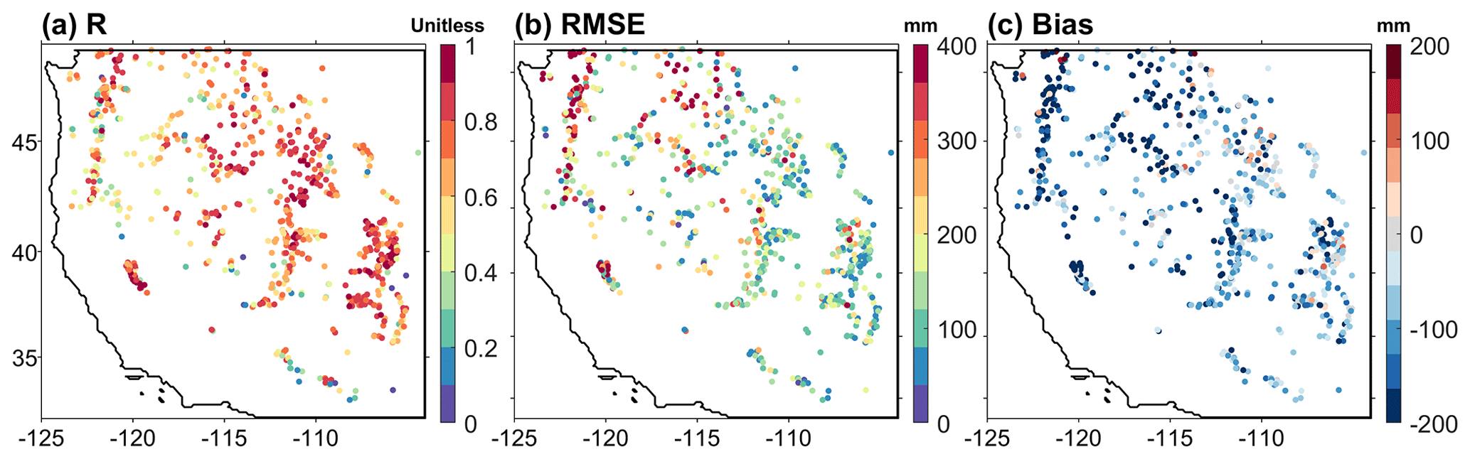
Figure 14Spatial distribution of statistical metrics of ELM performance against the field snow water equivalent (SWE) data from SNOTEL: (a) R, (b) bias, and (c) RMSE.
Compared to SNOTEL, UA presents a high correlation across sites (Fig. 14), with the mean R values being 0.69. The mean RMSE of ELM is 189.6 mm, the Cascades Range shows larger RMSE values than other regions. ELM underestimates SWE nearly across all sites, with the mean biases of −122.7 mm. The biases of the meteorological forcing in NLDAS-2 and the spatial-scale mismatch between the point-scale SNOTEL and the grid-level ELM simulations can contribute to uncertainty in the comparison.

Figure 15Spatial distributions of (a, d, g, j, m) snow timing, and (b–c, e, f, h, i, k, l, n–o) the snow timing difference between ELM and two remote sensing products (i.e., STC-MODSCAG and SPIReS). Five snow timing metrics are included: (a–c) Accumulation_onset_date, (d–f) Depletion_onset_date, (g–i) Midpoint_date, (j–l) End_date, and (m–o) Duration. The regions with no successful retrievals of snow timing are masked with white color. The area-weighted average values are labeled in each figure.
3.2 Snow phenology
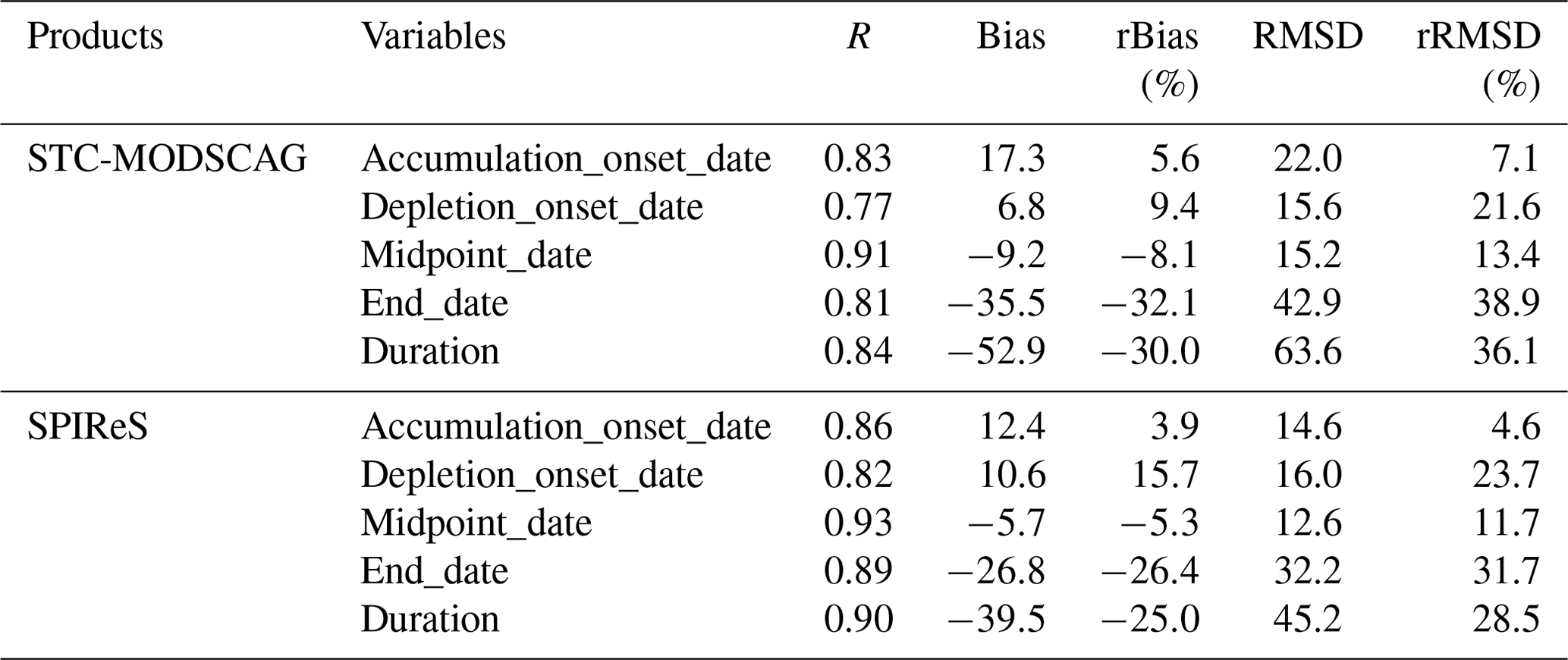
ELM well reproduces the snow phenology, compared to two remote sensing products (Figs. 15 and 16). As expected, over mountainous areas, ELM shows earlier snow onset, later depletion, and thus longer snow duration compared to flat and generally lower elevation areas (first column of Fig. 15). Compared to STC-MODSCAG and SPIReS (second and third columns of Fig. 15), ELM shows later Accumulation_onset_date over the whole WUS with a mean bias of +17.3 and +12.4 d, respectively, which may be caused by the bias in the meteorological forcing data of NLDAS-2 and the simple parameterizations of the partitioning of precipitation into rainfall or snowfall and has later Depletion_onset_date but earlier Midpoint_date and End_date. For instance, ELM melts off earlier with a mean bias of −35.5 and −26.8 d, respectively, than STC-MODSCAG and SPIReS, suggesting that ELM has higher snowmelt rate. Thus, ELM has a short snow duration with a mean bias of −52.9 and −39.5 d, respectively, compared to the two remote sensing products. The large biases exist in the western mountains for End_date (Fig. 15k, l, n, and o). Overall snow phenology in ELM has a high spatial correlation with that of the remote sensing products (Table 3). Although ELM overestimates Accumulation_onset_date and Depletion_onset_date and underestimates Midpoint_date, End_date, and Duration, ELM well captures the IAVs of all five snow phenology metrics (first column of Fig. 16), As the elevation increases, Accumulation_onset_date decreases, but the other four metrics increase for all the three datasets (second column of Fig. 16). ELM also has similar magnitudes and distributions for each elevation interval compared to the remote sensing products, while the three data show larger and larger differences with the increase of forest cover (third column of Fig. 16).
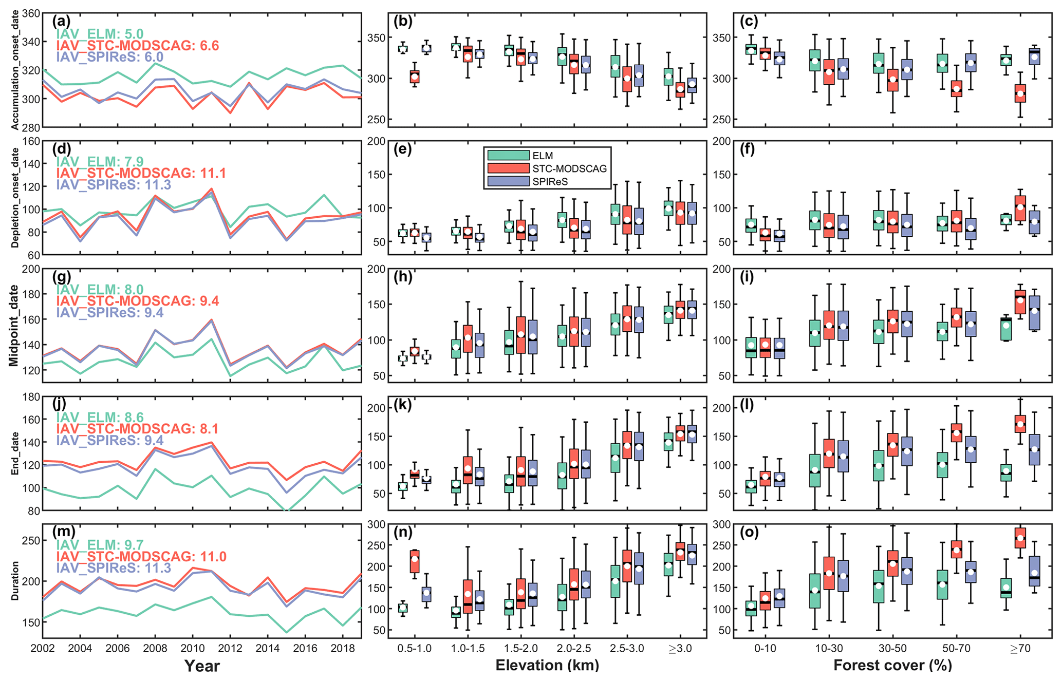
Figure 16(a, d, g, j, m) Time series of regional average values, (b, e, h, k, n) elevation gradients, and (c, f, i, l, o) change with forest cover of snow timing in ELM and two remote sensing products (i.e., STC-MODSCAG and SPIReS) for different metrics: (a–c) Accumulation_onset_date, (d–f) Depletion_onset_date, (g–i) Midpoint_date, (j–l) End_date, and (m–o) Duration over the WUS. The IAV values of different data are shown in (a, d, g, j, m). In panels (b, c, e, f, h, i, k, l, n, o), the white dots represent the average values.
Table 3Evaluation of snow phenology in ELM against STC-MODSCAG and SPIReS.
The evaluation results suggest an overall good performance of ELM in simulating snow properties, while some biases and uncertainties still exist, especially over mountainous areas with dense forest cover. Compared to the remote sensing products, ELM well reproduces the spatio-temporal pattern, interannual variabilities, and elevation gradients of fsno and αsur (Figs. 3–6), but large biases exist in Rocky Mountains and Sierra Nevada for αsur (Figs. 3 and 5). There are still large spatio-temporal inconsistencies of αsno, Ssno, and Rsno among ELM, STC-MODSCAG, and SPIReS (Figs. 8–11 and S6–S9). The underestimation of SWE and snow depth by ELM is comparable to the reported results based on CLM4 (Toure et al., 2016, 2018). The NLDAS-2 data used in the ELM simulations have large negative precipitation biases and high air temperature uncertainties over high-elevation terrain compared to both field measurements and PRISM over the WUS (Henn et al., 2018; O'Neill et al., 2021; Pan et al., 2003; Schreiner-McGraw and Ajami, 2022), which can partly explain the negative SWE bias in ELM. Besides, a 0.125∘ grid may have high subgrid variabilities of snow, especially in mountainous areas (Meromy et al., 2013), and SNOTEL stations in mountains located on flat surface may not capture the subgrid spatial variabilities (Toure et al., 2016). Overall ELM can well track the snow phenology but shows a late start of snow accumulation in winter. This is consistent with the underestimation of SWE and may be related to the precipitation and air temperature bias in the meteorological forcing data of NLDAS-2 and the partitioning of precipitation into rainfall or snowfall in ELM. An earlier snowmelt is also found in ELM, and there are similar issues in other LSMs, e.g., CLM4 (Toure et al., 2018) and Noah with multi-parameterization (Noah-MP) (Xiao et al., 2021). Note that in this study, we defined snow season and phenology based on fsno rather than SWE, and thus how ELM captures the date of peak snowpack, snowmelt timing, and snowmelt rate needs further investigation based on SWE.
There are still some uncertainties in the benchmarking datasets used in this study. First, the MCD43 product performs well in representing αsur during snow cover periods but may have poor performance for ephemeral snow due to its assumptions of stable land surface status within 16 d (Wang et al., 2012, 2014). Besides, frequent cloud cover and a lack of explicit representations of topographic effects can affect the accuracy of the MCD43 product over mountainous areas (Hao et al., 2018a, b, 2019). There are some inconsistencies between STC-MODSCAG and SPIReS (Figs. 3 and 4) due to the different algorithms and data processing (e.g., interpolation and filtering). Although the physically-based STC-MODSCAG and SPIReS provide higher quality unbiased fsno estimates than the MOD10A1 snow product, based on empirical algorithms against field measurements across different forest cover, snow cover, snow climate and viewing angles (Bair et al., 2021b; Rittger et al., 2013; Stillinger et al., 2022), the issues of reflectance errors, one to many problems intrinsic to spectral unmixing, cloud contamination, topographic shadows, sun-sensor geometric effects, and the impacts of forest cover can still affect their reliabilities (Bair et al., 2022; Raleigh et al., 2013; Stillinger et al., 2022). These issues can also affect the accuracy of extracted snow phenology (Sect. 2.4). Uncertainties of Ssno and Rsno in STC-MODSCAG/STC-MODDRFS and SPIReS exist (Bair et al., 2019). In summary, the heterogeneity of snow within pixels, relatively low spectral resolution, and interference from clouds limits the diagnostic capabilities of snow properties from MODIS. Ongoing and upcoming hyperspectral remote sensing missions (e.g., the recently launched Environmental Mapping and Analysis Program (https://www.enmap.org/, last access: 4 February 2023) and NASA's Surface Biology and Geology (Cawse-Nicholson et al., 2021) will enhance the abilities of remote sensing to monitor snow properties. There are also some discrepancies between UA and SNODAS (Figs. 11 and 12). The uncertainties in the PRISM data over complex terrain (Henn et al., 2018) may degrade the performance of UA. Compared to ground survey data, SWE in SNODAS over alpine areas has degraded performance due to the neglect of wind redistribution of snow (Clow et al., 2012). Compared to GPS interferometric reflectometry snow depth data, SNODAS still needs to be improved over complex terrain and areas with high vegetation heterogeneities (Boniface et al., 2015). The independent comparisons also have shown the underestimations and overestimations of SNODAS (Bair et al., 2016; Dozier, 2011; Dozier et al., 2016). Developing reliable benchmarking datasets for advancing snow modeling is still challenging but necessary (Ménard et al., 2019).
There is significant room for improving simulations of snow processes in ELM, ranging from the input forcing data to parameter settings and model structure. Meteorological forcing data have been demonstrated to have large impacts on snow simulations (Günther et al., 2019). The NLDAS-2 forcing data were used to drive ELM in the study, which is rather coarse to represent the subgrid heterogeneity of precipitation over mountainous areas (Tesfa et al., 2020). Although NLDAS-2 has many improvements compared to NLDAS-1 (Xia et al., 2012), there are still some spatio-temporal discontinuities in the precipitation of NLDAS-2 (Ferguson and Mocko, 2017; Xia et al., 2019). Besides, there are still some documented systematic precipitation and air temperature biases in NLDAS-2, especially over mountainous areas (Henn et al., 2018; O'Neill et al., 2021; Pan et al., 2003). The climatological aerosol deposition data used in the ELM simulations are too coarse to capture the fine-scale spatial variations of BC and dust, which limits the accuracy of simulated Rsno and thus αsno. The model structures used in different LSMs have different complexities, assumptions, and simplifications (Lee et al., 2021; Magnusson et al., 2015). In ELM, some snow processes are modeled empirically, and some parameters were set empirically or from the literature, which may contain large uncertainties. For instance, in the ELM snow albedo model, spherical snow grain shape, internal mixing of BC snow and external mixing of dust snow are default settings, which may be oversimplified (Hao et al., 2022) and can potentially affect the accuracy of Rsno and αsno. The large uncertainty of Ssno is relevant to the unrealistic snow aging representations in ELM (Qian et al., 2014), which can further affect αsno. The bias of αsno can further affect the accuracy of absorbed energy by snow and αsur (contains the contributions from snow and non-snow vegetation/soil), and thus the change of SWE and Dsno. The uncertainties of SWE can further propagate to fsno, because ELM uses SWE to estimate fsno (Swenson and Lawrence, 2012). In the snow cover parameterization of ELM, snow accumulation ratio and snowmelt shape factor are empirically set as fixed values without spatio-temporal variations (Swenson and Lawrence, 2012), which can also affect the accuracy of fsno. The snow cover over complex terrain was simply parameterized as a function of the standard deviation of elevation, which may explain the large biases of fsno (Fig. 3) over mountainous areas (Swenson and Lawrence, 2012). All of these uncertainties contribute to the bias of snow phenology in ELM (Sect. 3.2). Besides, some important processes are missing in ELM, such as the snow redistribution and sublimation by blowing snow (Xie et al., 2019), and the interaction between vegetation and snow, which possibly lead to the degraded performance of ELM (Sect. 3). Developing accurate forcing data, improving/choosing suitable snow models/parameterizations, and calibrating/optimizing model parameters are all important for accurate simulations of snow processes in LSMs.
Further studies are needed to conduct systematic diagnosis and attributions of ELM simulation biases and evaluate the ability of ELM in capturing the long-term trends and climate effects of snow. Attributing the snow simulation biases to the specific parameterizations or processes is still challenging but necessary to identify and locate the major sources of errors. Because the snow processes are coupled and impacted by each other, further sensitivity analysis and numerical experiments varying factors one at a time are needed. An international coordinated project of the intercomparison of snow schemes in Earth system models, ESM-SNOWMIP, provides a good opportunity for ELM to identify crucial processes leading to large biases in simulated snow and compare with other LSMs from local to global scales (Krinner et al., 2018; Menard et al., 2021). In this study, we found no significant increasing or decreasing trend of snow from 2001 to 2019 over the WUS for both ELM and other benchmarking datasets. However, 19 years are not long enough to characterize long-term trends of snow, and analysis was not performed on discrete a river basin or elevation subsets that may be experiencing change nor during the JJA time period. To reduce the impacts of the uncertainties from atmospheric forcing, this study focused on evaluating the offline ELM simulations forced by NLDAS-2, since errors in both simulated temperature and precipitation have been recognized as the main drivers of snowpack errors in E3SM (Brunke et al., 2021). However, snow-related land–atmosphere interactions are neglected in the land-only simulations. Additional studies are required to evaluate E3SM's ability to capture the impacts of snow on regional climate by performing coupled E3SM simulations with an active land and atmosphere model.
Snow over the WUS plays an important role in regional climate, hydrological and ecological systems, and human society. This study systematically evaluated the snow properties (including αsur, αsno, fsno, Ssno, Rsno, SWE, and Dsno) and snow phenology (including four snow dates and one snow duration) simulated by ELM using SNOTEL field measurements, MODIS remote sensing products, and two data assimilation products. Overall, the ELM snow simulations agree well with the benchmarking datasets in terms of spatio-temporal distributions, interannual variabilities, and elevation gradients for different snow properties. However, ELM has large biases of fsno for dense forest cover and αsur in the Rocky Mountains and Sierra Nevada, while underestimating SWE and Dsno, especially over mountainous areas with dense forest cover for both winter and spring. The ELM simulations show large inconsistencies with the remote sensing retrievals of αsno, Ssno, and Rsno. Compared to SNOTEL, ELM has larger negative biases of SWE, probably because there are some systematic biases of precipitation and air temperature in NLDAS-2. Besides, there is a large spatial-scale mismatch between point-scale field measurements and grid-level simulations, which can contribute to the large biases of ELM. There are also some inconsistencies of snow phenology between ELM and remote sensing products, with ELM showing later snow onset, earlier depletion, and shorter snow duration, consistent with the underestimation of SWE. This study documents the ELM performance in simulating snow processes and demonstrates the necessity for further improving the snow properties and snow phenology represented in LSMs. Further efforts are needed to improve the accuracy of snow properties, especially Ssno and Rsno in both ELM simulations and remote sensing retrievals, and resolve the early melt-off of snow in spring and underestimations of SWE in ELM, especially over the complex terrain of the WUS.
Table A2Overview of some typical studies and this study on the evaluation of snow processes in land surface models (LSMs).
ELM model codes with new updates used in the study are publicly available at https://doi.org/10.5281/zenodo.6324131 (Hao, 2022a). All the SRTM DEM, and GFCC forest cover and MCD43 surface albedo data can be freely downloaded from the Google Earth Engine (https://earthengine.google.com; GEE team, 2023) (Gorelick et al., 2017). The STC-MODSCAG/STC-MODDRFS and SPIReS data used in the study are available at https://doi.org/10.5281/zenodo.7194703 (Hao, 2022b). The SPIReS code is publicly available at https://github.com/edwardbair/SPIRES (Bair, 2023). UA and SNODAS data can be accessed at https://doi.org/10.5067/0GGPB220EX6A (Broxton et al., 2019) and https://doi.org/10.7265/N5TB14TC (National Operational Hydrologic Remote Sensing Center, 2004), respectively. BCQC SNOTEL data are available at https://www.pnnl.gov/data-products (Sun and Wigmosta, 2023; Sun et al., 2019; Yan et al., 2018). Codes to process data, generate all results, and produce all figures are archived at https://doi.org/10.5281/zenodo.7607813 (Hao, 2023).
The supplement related to this article is available online at: https://doi.org/10.5194/tc-17-673-2023-supplement.
DH conceived the study, designed the experiments, collected the evaluation data, conducted the simulations, analyzed the results, and drafted the original paper. GB conceived the study, designed the experiments, discussed the results, and edited the paper. EB, KR, and TS provided the remote sensing data and edited the paper. YG and LRL discussed the results and edited the paper. All authors contributed to reviewing and improving the paper.
At least one of the (co-)authors is a member of the editorial board of The Cryosphere. The peer-review process was guided by an independent editor, and the authors have no other competing interests to declare.
Publisher's note: Copernicus Publications remains neutral with regard to jurisdictional claims in published maps and institutional affiliations.
This research was conducted at Pacific Northwest National Laboratory, which is operated for the US Department of Energy by Battelle Memorial Institute under contract DEAC05-76RL01830. This research used resources of the National Energy Research Scientific Computing Center (NERSC), a DOE Office of Science User Facility supported by the Office of Science of the US Department of Energy under contract no. DE-AC02-15 05CH11231. The reported research also used DOE's Biological and Environmental Research Earth System Modeling program's Compy computing cluster located at Pacific Northwest National Laboratory. Dalei Hao thanks his wife Meng Luo for all her love and support.
This research has been supported by the US Department of Energy, Office of Science, Office of Biological and Environmental Research, Earth System Model Development program area, as part of the Climate Process Team projects and the US National Oceanic and Atmospheric Administration (NOAA, grant nos. NOAA-OAR-CPO-2019-2005530 and NA19OAR4310243). Support was also provided by NASA grant nos. 80NSSC20K1349, 80NSSC18K0427, NSSC22K0703, 80NSSC21K0997, and 80NSSC20K1722. Yu Gu acknowledges support by (while serving at) the National Science Foundation.
This paper was edited by Alexandre Langlois and reviewed by two anonymous referees.
Anttila, K., Manninen, T., Jääskeläinen, E., Riihelä, A., and Lahtinen, P.: The Role of Climate and Land Use in the Changes in Surface Albedo Prior to Snow Melt and the Timing of Melt Season of Seasonal Snow in Northern Land Areas of 40∘ N–80∘ N during 1982–2015, Remote Sens., 10, 1619, https://doi.org/10.3390/rs10101619, 2018.
Bair, E. H., Rittger, K., Davis, R. E., Painter, T. H., and Dozier, J.: Validating reconstruction of snow water equivalent in California's Sierra Nevada using measurements from the NASA Airborne Snow Observatory, Water Resour. Res., 52, 8437–8460, 2016.
Bair, E. H., Rittger, K., Skiles, S. M., and Dozier, J.: An Examination of Snow Albedo Estimates From MODIS and Their Impact on Snow Water Equivalent Reconstruction, Water Resour. Res., 55, 7826–7842, 2019.
Bair, E.: edwardbair/SPIRES, GitHub [code], https://github.com/edwardbair/SPIRES, last access: 4 February 2023.
Bair, E., Stillinger, T., Rittger, K., and Skiles, M.: COVID-19 lockdowns show reduced pollution on snow and ice in the Indus River Basin, P. Natl. Acad. Sci. USA, 118, e2101174118, https://doi.org/10.1073/pnas.2101174118, 2021a.
Bair, E. H., Stillinger, T., and Dozier, J.: Snow Property Inversion From Remote Sensing (SPIReS): A Generalized Multispectral Unmixing Approach With Examples From MODIS and Landsat 8 OLI, IEEE T. Geosci. Remote, 59, 7270–7284, 2021b.
Bair, E. H., Dozier, J., Stern, C., LeWinter, A., Rittger, K., Savagian, A., Stillinger, T., and Davis, R. E.: Divergence of apparent and intrinsic snow albedo over a season at a sub-alpine site with implications for remote sensing, The Cryosphere, 16, 1765–1778, https://doi.org/10.5194/tc-16-1765-2022, 2022.
Barnett, T. P., Adam, J. C., and Lettenmaier, D. P.: Potential impacts of a warming climate on water availability in snow-dominated regions, Nature, 438, 303–309, 2005.
Berghuijs, W. R., Woods, R. A., and Hrachowitz, M.: A precipitation shift from snow towards rain leads to a decrease in streamflow, Nat. Clim. Change, 4, 583–586, 2014.
Boniface, K., Braun, J. J., McCreight, J. L., and Nievinski, F. G.: Comparison of Snow Data Assimilation System with GPS reflectometry snow depth in the Western United States, Hydrol. Process., 29, 2425–2437, 2015.
Böttcher, K., Aurela, M., Kervinen, M., Markkanen, T., Mattila, O.-P., Kolari, P., Metsämäki, S., Aalto, T., Arslan, A. N., and Pulliainen, J.: MODIS time-series-derived indicators for the beginning of the growing season in boreal coniferous forest – A comparison with CO2 flux measurements and phenological observations in Finland, Remote Sens. Environ., 140, 625–638, 2014.
Broxton, P., Zeng, X., and Dawson, N.: Daily 4 km gridded SWE and snow depth from assimilated in-situ and modeled data over the conterminous US, version 1, NASA National Snow and Ice Data Center Distributed Active Archive Center, Boulder, CO [data set], https://doi.org/10.5067/0GGPB220EX6A, 2019.
Brunke, M. A., Welty, J., and Zeng, X.: Attribution of Snowpack Errors to Simulated Temperature and Precipitation in E3SMv1 Over the Contiguous United States, J. Adv. Model. Earth Syst., 13, e2021MS002640, https://doi.org/10.1029/2021MS002640, 2021.
Brutel-Vuilmet, C., Ménégoz, M., and Krinner, G.: An analysis of present and future seasonal Northern Hemisphere land snow cover simulated by CMIP5 coupled climate models, The Cryosphere, 7, 67–80, https://doi.org/10.5194/tc-7-67-2013, 2013.
Cawse-Nicholson, K., Townsend, P. A., Schimel, D., Assiri, A. M., Blake, P. L., Buongiorno, M. F., Campbell, P., Carmon, N., Casey, K. A., Correa-Pabón, R. E., Dahlin, K. M., Dashti, H., Dennison, P. E., Dierssen, H., Erickson, A., Fisher, J. B., Frouin, R., Gatebe, C. K., Gholizadeh, H., Gierach, M., Glenn, N. F., Goodman, J. A., Griffith, D. M., Guild, L., Hakkenberg, C. R., Hochberg, E. J., Holmes, T. R. H., Hu, C., Hulley, G., Huemmrich, K. F., Kudela, R. M., Kokaly, R. F., Lee, C. M., Martin, R., Miller, C. E., Moses, W. J., Muller-Karger, F. E., Ortiz, J. D., Otis, D. B., Pahlevan, N., Painter, T. H., Pavlick, R., Poulter, B., Qi, Y., Realmuto, V. J., Roberts, D., Schaepman, M. E., Schneider, F. D., Schwandner, F. M., Serbin, S. P., Shiklomanov, A. N., Stavros, E. N., Thompson, D. R., Torres-Perez, J. L., Turpie, K. R., Tzortziou, M., Ustin, S., Yu, Q., Yusup, Y., and Zhang, Q.: NASA's surface biology and geology designated observable: A perspective on surface imaging algorithms, Remote Sens. Environ., 257, 112349, https://doi.org/10.1016/j.rse.2021.112349, 2021.
Chen, X., Liang, S., Cao, Y., He, T., and Wang, D.: Observed contrast changes in snow cover phenology in northern middle and high latitudes from 2001–2014, Scient. Rep., 5, 16820, https://doi.org/10.1038/srep16820, 2015.
Clow, D. W., Nanus, L., Verdin, K. L., and Schmidt, J.: Evaluation of SNODAS snow depth and snow water equivalent estimates for the Colorado Rocky Mountains, USA, Hydrol. Process., 26, 2583–2591, 2012.
Dang, C., Zender, C. S., and Flanner, M. G.: Intercomparison and improvement of two-stream shortwave radiative transfer schemes in Earth system models for a unified treatment of cryospheric surfaces, The Cryosphere, 13, 2325–2343, https://doi.org/10.5194/tc-13-2325-2019, 2019.
Dawson, N., Broxton, P., and Zeng, X.: Evaluation of Remotely Sensed Snow Water Equivalent and Snow Cover Extent over the Contiguous United States, J. Hydrometeorol., 19, 1777–1791, 2018.
Decharme, B., Brun, E., Boone, A., Delire, C., Le Moigne, P., and Morin, S.: Impacts of snow and organic soils parameterization on northern Eurasian soil temperature profiles simulated by the ISBA land surface model, The Cryosphere, 10, 853–877, https://doi.org/10.5194/tc-10-853-2016, 2016.
Dietz, A. J., Kuenzer, C., Gessner, U., and Dech, S.: Remote sensing of snow – a review of available methods, Int. J. Remote Sens., 33, 4094–4134, 2012.
Dong, C.: Remote sensing, hydrological modeling and in situ observations in snow cover research: A review, J. Hydrol., 561, 573–583, 2018.
Dozier, J.: Mountain hydrology, snow color, and the fourth paradigm, Eos Trans. Am. Geophys. Union, 92, 373–374, 2011.
Dozier, J., Painter, T. H., Rittger, K., and Frew, J. E.: Time–space continuity of daily maps of fractional snow cover and albedo from MODIS, Adv. Water Resour., 31, 1515–1526, 2008.
Dozier, J., Bair, E. H., and Davis, R. E.: Estimating the spatial distribution of snow water equivalent in the world's mountains, WIREs Water, 3, 461–474, 2016.
Ferguson, C. R. and Mocko, D. M.: Diagnosing an Artificial Trend in NLDAS-2 Afternoon Precipitation, J. Hydrometeorol., 18, 1051–1070, 2017.
Flanner, M. G., Zender, C. S., Randerson, J. T., and Rasch, P. J.: Present-day climate forcing and response from black carbon in snow, J. Geophys. Res.-Atmos., 112, D11202, https://doi.org/10.1029/2006JD008003, 2007.
Flanner, M. G., Shell, K. M., Barlage, M., Perovich, D. K., and Tschudi, M. A.: Radiative forcing and albedo feedback from the Northern Hemisphere cryosphere between 1979 and 2008, Nat. Geosci., 4, 151–155, 2011.
GEE team: A planetary-scale platform for Earth science data & analysis, https://earthengine.google.com, last access: 5 February 2023.
Golaz, J.-C., Caldwell, P. M., Van Roekel, L. P., Petersen, M. R., Tang, Q., Wolfe, J. D., Abeshu, G., Anantharaj, V., Asay-Davis, X. S., Bader, D. C., Baldwin, S. A., Bisht, G., Bogenschutz, P. A., Branstetter, M., Brunke, M. A., Brus, S. R., Burrows, S. M., Cameron-Smith, P. J., Donahue, A. S., Deakin, M., Easter, R. C., Evans, K. J., Feng, Y., Flanner, M., Foucar, J. G., Fyke, J. G., Griffin, B. M., Hannay, C., Harrop, B. E., Hoffman, M. J., Hunke, E. C., Jacob, R. L., Jacobsen, D. W., Jeffery, N., Jones, P. W., Keen, N. D., Klein, S. A., Larson, V. E., Leung, L. R., Li, H.-Y., Lin, W., Lipscomb, W. H., Ma, P.-L., Mahajan, S., Maltrud, M. E., Mametjanov, A., McClean, J. L., McCoy, R. B., Neale, R. B., Price, S. F., Qian, Y., Rasch, P. J., Reeves Eyre, J. E. J., Riley, W. J., Ringler, T. D., Roberts, A. F., Roesler, E. L., Salinger, A. G., Shaheen, Z., Shi, X., Singh, B., Tang, J., Taylor, M. A., Thornton, P. E., Turner, A. K., Veneziani, M., Wan, H., Wang, H., Wang, S., Williams, D. N., Wolfram, P. J., Worley, P. H., Xie, S., Yang, Y., Yoon, J.-H., Zelinka, M. D., Zender, C. S., Zeng, X., Zhang, C., Zhang, K., Zhang, Y., Zheng, X., Zhou, T., and Zhu, Q.: The DOE E3SM Coupled Model Version 1: Overview and Evaluation at Standard Resolution, J. Adv. Model. Earth Syst., 11, 2089–2129, 2019.
Gorelick, N., Hancher, M., Dixon, M., Ilyushchenko, S., Thau, D., and Moore, R.: Google Earth Engine: Planetary-scale geospatial analysis for everyone, Remote Sens. Environ., 202, 18–27, https://doi.org/10.1016/j.rse.2017.06.031, 2017.
Günther, D., Marke, T., Essery, R., and Strasser, U.: Uncertainties in Snowpack Simulations – Assessing the Impact of Model Structure, Parameter Choice, and Forcing Data Error on Point-Scale Energy Balance Snow Model Performance, Water Resour. Res., 55, 2779–2800, 2019.
Hamlet, A. F. and Lettenmaier, D. P.: Effects of 20th century warming and climate variability on flood risk in the western U.S., Water Resour. Res., 43, W06427, https://doi.org/10.1029/2006WR005099, 2007.
Hao, D.: daleihao/E3SM: ELM-SNOW (v1.1.0.0), Zenodo [code], https://doi.org/10.5281/zenodo.6324131, 2022a.
Hao, D.: MODIS daily snow data (STC-MODSCAG/STC-MODDRFS and SPIReS) over the Western US from 2001–2019, Zenodo [data set], https://doi.org/10.5281/zenodo.7194703, 2022b.
Hao, D.: daleihao/snow_evaluation_ELM: Codes for the ELM snow evaluation study (Version v1), Zenodo [code], https://doi.org/10.5281/zenodo.7607813, 2023.
Hao, D., Wen, J., Xiao, Q., Wu, S., Lin, X., Dou, B., You, D., and Tang, Y.: Simulation and Analysis of the Topographic Effects on Snow-Free Albedo over Rugged Terrain, Remote Sens., 10, 278, https://doi.org/10.3390/rs10020278, 2018a.
Hao, D., Wen, J., Xiao, Q., Wu, S., Lin, X., You, D., and Tang, Y.: Modeling Anisotropic Reflectance Over Composite Sloping Terrain, IEEE T. Geosci. Remote, 56, 3903–3923, 2018b.
Hao, D., Wen, J., Xiao, Q., Lin, X., You, D., Tang, Y., Liu, Q., and Zhang, S.: Sensitivity of Coarse-Scale Snow-Free Land Surface Shortwave Albedo to Topography, J. Geophys. Res.-Atmos., 124, 9028–9045, 2019.
Hao, D., Bisht, G., Gu, Y., Lee, W.-L., Liou, K.-N., and Leung, L. R.: A parameterization of sub-grid topographical effects on solar radiation in the E3SM Land Model (version 1.0): implementation and evaluation over the Tibetan Plateau, Geosci. Model Dev., 14, 6273–6289, https://doi.org/10.5194/gmd-14-6273-2021, 2021.
Hao, D., Bisht, G., Huang, M., Ma, P.-L., Tesfa, T., Lee, W.-L., Gu, Y., and Leung, L. R.: Impacts of Sub-Grid Topographic Representations on Surface Energy Balance and Boundary Conditions in the E3SM Land Model: A Case Study in Sierra Nevada, Journal of Advances in Modeling Earth Systems, 14, e2021MS002862, 2022.
Hao, D., Bisht, G., Rittger, K., Bair, E., He, C., Huang, H., Dang, C., Stillinger, T., Gu, Y., Wang, H., Qian, Y., and Leung, L. R.: Improving snow albedo modeling in the E3SM land model (version 2.0) and assessing its impacts on snow and surface fluxes over the Tibetan Plateau, Geosci. Model Dev., 16, 75–94, https://doi.org/10.5194/gmd-16-75-2023, 2023.
Henderson, G. R., Peings, Y., Furtado, J. C., and Kushner, P. J.: Snow–atmosphere coupling in the Northern Hemisphere, Nat. Clim. Change, 8, 954–963, 2018.
Henn, B., Newman, A. J., Livneh, B., Daly, C., and Lundquist, J. D.: An assessment of differences in gridded precipitation datasets in complex terrain, J. Hydrol., 556, 1205–1219, 2018.
Jiang, Y., Chen, F., Gao, Y., He, C., Barlage, M., and Huang, W.: Assessment of Uncertainty Sources in Snow Cover Simulation in the Tibetan Plateau, J. Geophys. Res.-Atmos., 125, e2020JD032674, https://doi.org/10.1029/2020JD032674, 2020.
Kouki, K., Anttila, K., Manninen, T., Luojus, K., Wang, L., and Riihelä, A.: Intercomparison of Snow Melt Onset Date Estimates From Optical and Microwave Satellite Instruments Over the Northern Hemisphere for the Period 1982–2015, J. Geophys. Res.-Atmos., 124, 11205–11219, 2019.
Krinner, G., Derksen, C., Essery, R., Flanner, M., Hagemann, S., Clark, M., Hall, A., Rott, H., Brutel-Vuilmet, C., Kim, H., Ménard, C. B., Mudryk, L., Thackeray, C., Wang, L., Arduini, G., Balsamo, G., Bartlett, P., Boike, J., Boone, A., Chéruy, F., Colin, J., Cuntz, M., Dai, Y., Decharme, B., Derry, J., Ducharne, A., Dutra, E., Fang, X., Fierz, C., Ghattas, J., Gusev, Y., Haverd, V., Kontu, A., Lafaysse, M., Law, R., Lawrence, D., Li, W., Marke, T., Marks, D., Ménégoz, M., Nasonova, O., Nitta, T., Niwano, M., Pomeroy, J., Raleigh, M. S., Schaedler, G., Semenov, V., Smirnova, T. G., Stacke, T., Strasser, U., Svenson, S., Turkov, D., Wang, T., Wever, N., Yuan, H., Zhou, W., and Zhu, D.: ESM-SnowMIP: assessing snow models and quantifying snow-related climate feedbacks, Geosci. Model Dev., 11, 5027–5049, https://doi.org/10.5194/gmd-11-5027-2018, 2018.
Lamarque, J.-F., Bond, T. C., Eyring, V., Granier, C., Heil, A., Klimont, Z., Lee, D., Liousse, C., Mieville, A., Owen, B., Schultz, M. G., Shindell, D., Smith, S. J., Stehfest, E., Van Aardenne, J., Cooper, O. R., Kainuma, M., Mahowald, N., McConnell, J. R., Naik, V., Riahi, K., and van Vuuren, D. P.: Historical (1850–2000) gridded anthropogenic and biomass burning emissions of reactive gases and aerosols: methodology and application, Atmos. Chem. Phys., 10, 7017–7039, https://doi.org/10.5194/acp-10-7017-2010, 2010.
Lee, W. Y., Gim, H.-J., and Park, S. K.: Review article: Parameterizations of snow-related physical processes in land surface models, The Cryosphere Discuss. [preprint], https://doi.org/10.5194/tc-2021-319, 2021.
Leung, L. R., Bader, D. C., Taylor, M. A., and McCoy, R. B.: An Introduction to the E3SM Special Collection: Goals, Science Drivers, Development, and Analysis, J. Adv. Model. Earth Syst., 12, e2019MS001821, https://doi.org/10.1029/2019MS001821, 2020.
Lundquist, J. D., Dickerson-Lange, S., Gutmann, E., Jonas, T., Lumbrazo, C., and Reynolds, D.: Snow interception modelling: Isolated observations have led to many land surface models lacking appropriate temperature sensitivities, Hydrol. Process., 35, e14274, https://doi.org/10.1002/hyp.14274, 2021.
Magnusson, J., Wever, N., Essery, R., Helbig, N., Winstral, A., and Jonas, T.: Evaluating snow models with varying process representations for hydrological applications, Water Resour. Res., 51, 2707–2723, 2015.
Mameno, K., Kubo, T., Oguma, H., Amagai, Y., and Shoji, Y.: Decline in the alpine landscape aesthetic value in a national park under climate change, Climatic Change, 170, 35, 2022.
Ménard, C. B., Essery, R., Barr, A., Bartlett, P., Derry, J., Dumont, M., Fierz, C., Kim, H., Kontu, A., Lejeune, Y., Marks, D., Niwano, M., Raleigh, M., Wang, L., and Wever, N.: Meteorological and evaluation datasets for snow modelling at 10 reference sites: description of in situ and bias-corrected reanalysis data, Earth Syst. Sci. Data, 11, 865–880, https://doi.org/10.5194/essd-11-865-2019, 2019.
Menard, C. B., Essery, R., Krinner, G., Arduini, G., Bartlett, P., Boone, A., Brutel-Vuilmet, C., Burke, E., Cuntz, M., Dai, Y., Decharme, B., Dutra, E., Fang, X., Fierz, C., Gusev, Y., Hagemann, S., Haverd, V., Kim, H., Lafaysse, M., Marke, T., Nasonova, O., Nitta, T., Niwano, M., Pomeroy, J., Schädler, G., Semenov, V. A., Smirnova, T., Strasser, U., Swenson, S., Turkov, D., Wever, N., and Yuan, H.: Scientific and Human Errors in a Snow Model Intercomparison, B. Am. Meteorol. Soc., 102, E61–E79, 2021.
Meromy, L., Molotch, N. P., Link, T. E., Fassnacht, S. R., and Rice, R.: Subgrid variability of snow water equivalent at operational snow stations in the western USA, Hydrol. Process., 27, 2383–2400, 2013.
Metsämäki, S., Böttcher, K., Pulliainen, J., Luojus, K., Cohen, J., Takala, M., Mattila, O.-P., Schwaizer, G., Derksen, C., and Koponen, S.: The accuracy of snow melt-off day derived from optical and microwave radiometer data – A study for Europe, Remote Sens. Environ., 211, 1–12, 2018.
Musselman, K. N., Addor, N., Vano, J. A., and Molotch, N. P.: Winter melt trends portend widespread declines in snow water resources, Nat. Clim. Change, 11, 418–424, 2021.
Myneni, R. B., Hoffman, S., Knyazikhin, Y., Privette, J., Glassy, J., Tian, Y., Wang, Y., Song, X., Zhang, Y., and Smith, G.: Global products of vegetation leaf area and fraction absorbed PAR from year one of MODIS data, Remote Sens. Environ., 83, 214–231, 2002.
National Operational Hydrologic Remote Sensing Center: Snow Data Assimilation System (SNODAS) Data Products at NSIDC, Version 1, NSIDC – National Snow and Ice Data Center, Boulder, Colorado, USA [data set], https://doi.org/10.7265/N5TB14TC, 2004.
Niittynen, P., Heikkinen, R. K., and Luoto, M.: Snow cover is a neglected driver of Arctic biodiversity loss, Nat. Clim. Change, 8, 997–1001, 2018.
O'Neill, M. M. F., Tijerina, D. T., Condon, L. E., and Maxwell, R. M.: Assessment of the ParFlow–CLM CONUS 1.0 integrated hydrologic model: evaluation of hyper-resolution water balance components across the contiguous United States, Geosci. Model Dev., 14, 7223–7254, https://doi.org/10.5194/gmd-14-7223-2021, 2021.
Painter, T. H., Rittger, K., McKenzie, C., Slaughter, P., Davis, R. E., and Dozier, J.: Retrieval of subpixel snow covered area, grain size, and albedo from MODIS, Remote Sens. Environ., 113, 868–879, 2009.
Painter, T. H., Bryant, A. C., and Skiles, S. M.: Radiative forcing by light absorbing impurities in snow from MODIS surface reflectance data, Geophys. Res. Lett., 39, L17502, https://doi.org/10.1029/2012GL052457, 2012.
Pan, M., Sheffield, J., Wood, E. F., Mitchell, K. E., Houser, P. R., Schaake, J. C., Robock, A., Lohmann, D., Cosgrove, B., Duan, Q., Luo, L., Higgins, R. W., Pinker, R. T., and Tarpley, J. D.: Snow process modeling in the North American Land Data Assimilation System (NLDAS): 2. Evaluation of model simulated snow water equivalent, J. Geophys. Res.-Atmos., 108, 8850, https://doi.org/10.1029/2003JD003994, 2003.
Peng, S., Piao, S., Ciais, P., Friedlingstein, P., Zhou, L., and Wang, T.: Change in snow phenology and its potential feedback to temperature in the Northern Hemisphere over the last three decades, Environ. Res. Lett., 8, 014008, https://doi.org/10.1088/1748-9326/8/1/014008, 2013.
Qian, Y., Wang, H., Zhang, R., Flanner, M. G., and Rasch, P. J.: A sensitivity study on modeling black carbon in snow and its radiative forcing over the Arctic and Northern China, Environ. Res. Lett., 9, 064001, https://doi.org/10.1088/1748-9326/9/6/064001, 2014.
Rabus, B., Eineder, M., Roth, A., and Bamler, R.: The shuttle radar topography mission – a new class of digital elevation models acquired by spaceborne radar, ISPRS J. Photogram. Remote Sens., 57, 241–262, 2003.
Räisänen, P., Makkonen, R., Kirkevåg, A., and Debernard, J. B.: Effects of snow grain shape on climate simulations: sensitivity tests with the Norwegian Earth System Model, The Cryosphere, 11, 2919–2942, https://doi.org/10.5194/tc-11-2919-2017, 2017.
Raleigh, M. S., Rittger, K., Moore, C. E., Henn, B., Lutz, J. A., and Lundquist, J. D.: Ground-based testing of MODIS fractional snow cover in subalpine meadows and forests of the Sierra Nevada, Remote Sens. Environ., 128, 44–57, 2013.
Rittger, K., Painter, T. H., and Dozier, J.: Assessment of methods for mapping snow cover from MODIS, Adv. Water Resour., 51, 367–380, 2013.
Rittger, K., Raleigh, M. S., Dozier, J., Hill, A. F., Lutz, J. A., and Painter, T. H.: Canopy Adjustment and Improved Cloud Detection for Remotely Sensed Snow Cover Mapping, Water Resour. Res., 56, e2019WR024914, https://doi.org/10.1029/2019WR024914, 2020.
Rittger, K., Brodzik, M. J., and Raleigh, M.: Snow Today, National Snow and Ice Data Center, Boulder, Colorado, USA, https://nsidc.org/snow-today/snow-viewer (last access: 4 February 2023), 2022.
Schaaf, C. B., Gao, F., Strahler, A. H., Lucht, W., Li, X., Tsang, T., Strugnell, N. C., Zhang, X., Jin, Y., Muller, J.-P., Lewis, P., Barnsley, M., Hobson, P., Disney, M., Roberts, G., Dunderdale, M., Doll, C., d'Entremont, R. P., Hu, B., Liang, S., Privette, J. L., and Roy, D.: First operational BRDF, albedo nadir reflectance products from MODIS, Remote Sens. Environ., 83, 135–148, 2002.
Schreiner-McGraw, A. P. and Ajami, H.: Combined impacts of uncertainty in precipitation and air temperature on simulated mountain system recharge from an integrated hydrologic model, Hydrol. Earth Syst. Sci., 26, 1145–1164, https://doi.org/10.5194/hess-26-1145-2022, 2022.
Serreze, M. C., Clark, M. P., Armstrong, R. L., McGinnis, D. A., and Pulwarty, R. S.: Characteristics of the western United States snowpack from snowpack telemetry (SNOTEL) data, Water Resour. Res., 35, 2145–2160, 1999.
Sexton, J. O., Song, X.-P., Feng, M., Noojipady, P., Anand, A., Huang, C., Kim, D.-H., Collins, K. M., Channan, S., DiMiceli, C., and Townshend, J. R.: Global, 30-m resolution continuous fields of tree cover: Landsat-based rescaling of MODIS vegetation continuous fields with lidar-based estimates of error, Int. J. Digit. Earth, 6, 427–448, 2013.
Siirila-Woodburn, E. R., Rhoades, A. M., Hatchett, B. J., Huning, L. S., Szinai, J., Tague, C., Nico, P. S., Feldman, D. R., Jones, A. D., Collins, W. D., and Kaatz, L.: A low-to-no snow future and its impacts on water resources in the western United States, Nat. Rev. Earth Environ., 2, 800–819, 2021.
Skiles, S. M., Flanner, M., Cook, J. M., Dumont, M., and Painter, T. H.: Radiative forcing by light-absorbing particles in snow, Nat. Clim. Change, 8, 964–971, 2018.
Stillinger, T., Rittger, K., Raleigh, M. S., Michell, A., Davis, R. E., and Bair, E. H.: Landsat, MODIS, and VIIRS snow cover mapping algorithm performance as validated by airborne lidar datasets, The Cryosphere Discuss. [preprint], https://doi.org/10.5194/tc-2022-159, in review, 2022.
Sun, N. and Wigmosta, M.: Data Products, https://www.pnnl.gov/data-products, last access: 5 February 2023.
Sun, N., Yan, H., Wigmosta, M. S., Leung, L. R., Skaggs, R., and Hou, Z.: Regional Snow Parameters Estimation for Large-Domain Hydrological Applications in the Western United States, J. Geophys. Res.- Atmos., 124, 5296–5313, https://doi.org/10.1029/2018JD030140, 2019.
Swenson, S. C. and Lawrence, D. M.: A new fractional snow-covered area parameterization for the Community Land Model and its effect on the surface energy balance, J. Geophys. Res.-Atmos., 117, D21107, https://doi.org/10.1029/2012JD018178, 2012.
Takala, M., Pulliainen, J., Metsamaki, S. J., and Koskinen, J. T.: Detection of Snowmelt Using Spaceborne Microwave Radiometer Data in Eurasia From 1979 to 2007, IEEE T. Geosci. Remote, 47, 2996–3007, 2009.
Tesfa, T. K., Leung, L. R., and Ghan, S. J.: Exploring Topography-Based Methods for Downscaling Subgrid Precipitation for Use in Earth System Models, J. Geophys. Res.-Atmos., 125, e2019JD031456, https://doi.org/10.1029/2019JD031456, 2020.
Toure, A. M., Rodell, M., Yang, Z.-L., Beaudoing, H., Kim, E., Zhang, Y., and Kwon, Y.: Evaluation of the Snow Simulations from the Community Land Model, Version 4 (CLM4), J. Hydrometeorol., 17, 153–170, 2016.
Toure, A. M., Luojus, K., Rodell, M., Beaudoing, H., and Getirana, A.: Evaluation of Simulated Snow and Snowmelt Timing in the Community Land Model Using Satellite-Based Products and Streamflow Observations, J. Adv. Model. Earth Syst., 10, 2933–2951, 2018.
Verseghy, D., Brown, R., and Wang, L.: Evaluation of CLASS Snow Simulation over Eastern Canada, J. Hydrometeorol., 18, 1205–1225, 2017.
Wang, H., Easter, R. C., Zhang, R., Ma, P.-L., Singh, B., Zhang, K., Ganguly, D., Rasch, P. J., Burrows, S. M., Ghan, S. J., Lou, S., Qian, Y., Yang, Y., Feng, Y., Flanner, M., Leung, L. R., Liu, X., Shrivastava, M., Sun, J., Tang, Q., Xie, S., and Yoon, J.-H.: Aerosols in the E3SM Version 1: New Developments and Their Impacts on Radiative Forcing, J. Adv. Model. Earth Syst., 12, e2019MS001851, https://doi.org/10.1029/2019MS001851, 2020.
Wang, Z., Schaaf, C. B., Chopping, M. J., Strahler, A. H., Wang, J., Román, M. O., Rocha, A. V., Woodcock, C. E., and Shuai, Y.: Evaluation of Moderate-resolution Imaging Spectroradiometer (MODIS) snow albedo product (MCD43A) over tundra, Remote Sensing of Environment, 117, 264-280, 2012.
Wang, Z., Schaaf, C. B., Strahler, A. H., Chopping, M. J., Román, M. O., Shuai, Y., Woodcock, C. E., Hollinger, D. Y., and Fitzjarrald, D. R.: Evaluation of MODIS albedo product (MCD43A) over grassland, agriculture and forest surface types during dormant and snow-covered periods, Remote Sens. Environ., 140, 60–77, 2014.
Wang, Z., Schaaf, C. B., Sun, Q., Shuai, Y., and Román, M. O.: Capturing rapid land surface dynamics with Collection V006 MODIS BRDF/NBAR/Albedo (MCD43) products, Remote Sens. Environ., 207, 50–64, 2018.
Xia, Y., Mitchell, K., Ek, M., Sheffield, J., Cosgrove, B., Wood, E., Luo, L., Alonge, C., Wei, H., Meng, J., Livneh, B., Lettenmaier, D., Koren, V., Duan, Q., Mo, K., Fan, Y., and Mocko, D.: Continental-scale water and energy flux analysis and validation for the North American Land Data Assimilation System project phase 2 (NLDAS-2): 1. Intercomparison and application of model products, J. Geophys. Res., 117, D03109, https://doi.org/10.1029/2011JD016048, 2012.
Xia, Y., Hao, Z., Shi, C., Li, Y., Meng, J., Xu, T., Wu, X., and Zhang, B.: Regional and Global Land Data Assimilation Systems: Innovations, Challenges, and Prospects, J. Meteorol. Res., 33, 159–189, 2019.
Xiao, M., Mahanama, S. P., Xue, Y., Chen, F., and Lettenmaier, D. P.: Modeling Snow Ablation over the Mountains of the Western United States: Patterns and Controlling Factors, J. Hydrometeorol., 22, 297–311, 2021.
Xie, Z., Hu, Z., Ma, Y., Sun, G., Gu, L., Liu, S., Wang, Y., Zheng, H., and Ma, W.: Modeling Blowing Snow Over the Tibetan Plateau With the Community Land Model: Method and Preliminary Evaluation, J. Geophys. Res.-Atmos., 124, 9332–9355, 2019.
Yan, H., Sun, N., Wigmosta, M., Skaggs, R., Hou, Z., and Leung, R.: Next-Generation Intensity-Duration-Frequency Curves for Hydrologic Design in Snow-Dominated Environments, Water Resour. Res., 54, 1093–1108, 2018.
Zeng, X., Broxton, P., and Dawson, N.: Snowpack Change From 1982 to 2016 Over Conterminous United States, Geophys. Res. Lett., 45, 12940–12947, https://doi.org/10.1029/2018GL079621, 2018.