the Creative Commons Attribution 4.0 License.
the Creative Commons Attribution 4.0 License.
 | 12 Dec 2023
Impact of the Nares Strait sea ice arches on the long-term stability of the Petermann Glacier ice shelf
Qin Zhou
Tore Hattermann
Nina Kirchner
One of the last remaining floating tongues of the Greenland ice sheet (GrIS), the Petermann Glacier ice shelf (PGIS), is seasonally shielded from warm Atlantic water (AW) by the formation of sea ice arches in the Nares Strait. However, continued decline of the Arctic sea ice extent and thickness suggests that arch formation is likely to become anomalous, necessitating an investigation into the response of PGIS to a year-round mobile and thin sea ice cover. We use a high-resolution unstructured grid 3-D ocean–sea ice–ice shelf setup, featuring an improved sub-ice-shelf bathymetry and a realistic PGIS geometry, to investigate in unprecedented detail the implications of transitions in the Nares Strait sea ice regime, that is, from a thick and landfast sea ice regime to a mobile, and further, a thin and mobile sea ice regime, with regard to PGIS basal melt. In all three sea ice regimes, basal melt near the grounding line (GL) presents a seasonal increase during summer, driven by a higher thermal driving. The stronger melt overturning increases the friction velocity slightly downstream, where enhanced friction-driven turbulent mixing further increases the thermal driving, substantially increasing the local melt. As the sea ice cover becomes mobile and thin, wind and (additionally in winter) convectively upwelled AW from the Nares Strait enter the PGIS cavity. While its effect on basal melting is largely limited to the shallower (<200 m) drafts during winter, in summer it extends to the GL (ca. 600 m) depth. In the absence of an increase in thermal driving, increased melting under the deeper (>200 m) drafts in winter is solely driven by the increased vertical shear of a more energetic boundary layer current. A similar behaviour is noted when transitioning from a mobile to a thin mobile sea ice cover in summer, when increases in thermal driving are negligible and increases in melt are congruent with increases in friction velocity. These results suggest that the projected continuation of the warming of the Arctic Ocean until the end of the 21st century and the accompanying decline in the Arctic sea ice extent and thickness will amplify the basal melt of PGIS, impacting the long-term stability of the Petermann Glacier and its contribution to the future GrIS mass loss and sea level rise.
- Article
(30982 KB) - Full-text XML
- BibTeX
- EndNote


The Greenland ice sheet (GrIS) is currently the largest single contributor to barystatic sea level rise and is losing mass at accelerating rates (Chen et al., 2017; The IMBIE Team, 2020; Sasgen et al., 2020). This acceleration is related to the increasing amount of heat which the warmer subsurface Atlantic water (AW) supplies to the GrIS marine margin (Slater et al., 2019; Wood et al., 2021). Such additional oceanic heat causes enhanced basal melting and calving at marine terminating glacier fronts. The disintegration of ice shelves and associated loss of buttressing forces on the upstream inland ice masses can lead to glacier-wide dynamic thinning and flow acceleration (Hill et al., 2018; Aschwanden et al., 2019; Rückamp et al., 2019).
Along the northern GrIS margin, the “north” and “northeast” sectors analysed by Mouginot et al. (2019) hold an ice volume which, if melted, would cause global mean sea level to rise by 273 cm (ca. 37 % of the total GrIS contribution). Therefore, continued presence of the few remaining buttressing ice shelves along its margin is pivotal to the sectorial and the GrIS mass balance, and its contribution to future sea level changes. However, with expected increases in basal melting driven by the ocean's response to a future warming climate, the stability of these ice shelves becomes of great concern.
Petermann Glacier (PG) has the largest discharge of all glaciers in the “north” sector, viz. 11.7 ± 1.2 Gt yr−1, with a drainage basin stretching across 6 % of the GrIS by area (Hill et al., 2017; Mouginot et al., 2019). PG terminates with a floating ice shelf, the Petermann Glacier ice shelf (PGIS), into the Petermann Fjord (PF). PGIS is ca. 50 km long and its thickness ranges between ca. 150 m near the calving front to 600 m at the grounding line (GL), where it is ca. 20 km wide. PGIS has been extensively investigated following the two recent episodic large calving events in 2010 and 2012 (Falkner et al., 2011; Münchow et al., 2014). In particular, hydrographic surveys have documented the inflow of warm and saline modified AW into the PF and the PGIS cavity (Heuzé et al., 2017; Washam et al., 2018), where it drives basal melt and melt undercutting, and renders PGIS susceptible to calving. PF extends for ca. 90 km before opening into the Nares Strait, which is a ca. 500 km long and 30–50 km wide waterway separating northwest Greenland from Ellesmere Island, and bridging the Lincoln Sea and Baffin Bay (Fig. 1(a)). Heat and freshwater exchange between the Arctic Ocean and the western subpolar North Atlantic Ocean is facilitated through the Nares Strait (Kwok, 2005), influenced by fjord and ocean circulation and sea ice dynamics.
Sea ice covers the Nares Strait for most of the year, and observations since 1996 show that landfast winter sea ice aids the formation of ice arches which extend across the Nares Strait and thus reduce or cease ice drift through it. Typically, a northern ice arch forms near the Lincoln Sea entrance to the Nares Strait and/or a southern one near the Smith Sound/Kane Basin region, with interannual variability in exact location and duration, and associated variations in sea ice transport through the Nares Strait (Kwok, 2005; Kwok et al., 2010; Münchow, 2016; Ryan and Münchow, 2017; Moore et al., 2021) (Fig. 1(a)). During summer, sea ice is mobile for ca. 3 months. For a seasonal cycle of winter landfast sea ice and summer mobile sea ice, modelling of ice shelf–ocean interactions at the PGIS demonstrated that changes in ocean circulation induced by changes in sea ice mobility and the resulting upwelling of AW increased the modelled PGIS basal melt rates by 20 % (Shroyer et al., 2017).
In 2007, neither of the ice arches formed. Sea ice area and the flow of ice volume through the Robeson Channel were reported to be not only the highest, but also more than twice the annual mean over the years 1997–2009 (Kwok et al., 2010). In 2019, when both the ice arches again failed to form, ice area flux through the Robeson Channel flux gate exceeded the one reported from 2007. Yet, ice volume flux was smaller due to reduced sea ice thickness (Moore et al., 2021). The 2019 event was preceded by a collapse of the northern ice arch in May 2017 and its complete absence in 2018, during which the southern arch persisted only for a short period (Moore and McNeil, 2018; Moore et al., 2021). Notably, between 1997 and 2019, the time period during which ice arches were present in the Nares Strait decreased by 7 d yr−1 (Moore et al., 2021).
A continued decline in the Arctic sea ice thickness (Maslanik et al., 2011; Kwok, 2018; Kacimi and Kwok, 2022) and duration of ice arch formation, and the resulting increased outflow of the thick Arctic multiyear ice, further expedites the transition towards a thin (and mobile) sea ice cover and makes ice arch formation more unlikely. The loss of ice arches implies that the seasonal cycle of sea ice mobility in the Nares Strait ceases and that instead, year-round mobile sea ice conditions start to prevail (Moore et al., 2021). Moreover, such a scenario is expected to continue in the future as the Arctic sea ice continues to decline in extent and thickness, and the Arctic Ocean is projected to be sea ice free during at least one summer before 2050 CE (Wang and Overland, 2012; Meredith et al., 2019; Pörtner et al., 2019; Notz and SIMIP Community, 2020). Consequences that these changes may have on the oceanic heat transport (e.g. via air–sea thermal and haline buoyancy fluxes and momentum transfer) towards the PGIS cavity, with ramifications for the long term stability of the PGIS, remain largely unknown.
In this study, we use the Finite Volume Community Ocean Model (FVCOM) (Chen et al., 2007), amended by an ice shelf (Zhou and Hattermann, 2020) and a sea ice module (Prakash et al., 2022), to investigate the implications of long-term (i.e. several decades) climate warming induced changes in the Nares Strait sea ice regime on PGIS basal melt. Here, variations in both the sea ice mobility (dynamics), and sea ice concentration and thickness (thermodynamics), are examined. Our high-resolution unstructured grid σ coordinate 3-D ocean–sea ice–ice shelf setup is able to better resolve the irregular coastal geometry and steeply sloping seafloor topography, as well as smoothly represent the sloping PGIS base and preserve vertical resolution in the deeper parts of the PGIS cavity. Other noteworthy improvements over similar existing numerical setups include the implementation of a realistic ice shelf basal topography, an improved sub-ice-shelf bathymetry, as well as the implementation of a laterally resolved inner sill (Tinto et al., 2015) ca. 25 km from the GL. We find that climate-warming-driven transition towards a mobile and thin sea ice cover from a landfast and thick one could result in up to a two-thirds increase in ice shelf averaged melt. In such a scenario, wind and convectively upwelled warm AW from the Nares Strait enter the PGIS cavity. Importantly, under the deeper (draft >200 m) regions of PGIS, melting intensifies in a more turbulent cavity without any noticeable increase in thermal driving, evidencing that a stronger circulation alone would be sufficient to drive considerable increase in melt.
2.1 Model setup
2.1.1 Ice shelf module
The unstructured grid, free-surface, 3-D primitive equation Finite Volume Community Ocean Model (FVCOM) (Chen et al., 2007) has recently been amended by an ice shelf module that allows modelling of oceanic processes in ice shelf cavities bounded by complex coastal geometries and fjord bathymetry. A concise summary of the module is provided below and a detailed description can be found in Zhou and Hattermann (2020). For a freely floating ice shelf with a known draft, the module modifies the horizontal pressure gradient forces to account for the effect of ice shelf basal topography as the σ layers subduct below it. The top friction (generated by the ice shelf–ocean interface) is similar to the bottom (generated by the bathymetry) and is assumed to be quadratic (Table A1). Thermodynamically, the ocean is assumed to be perfectly insulated from the atmosphere by the ice shelf cover, and the melting and freezing processes at the ice shelf–ocean interface are parameterized using the three fundamental equations formulated in Holland and Jenkins (1999). The effective heat and virtual salt fluxes across the ice shelf–ocean interface are calculated following Jenkins et al. (2001) and applied as boundary conditions for temperature and salinity at the ice shelf base. For a given set of far field ocean boundary conditions (see Sect. 2.2 below), thermodynamics at the ice shelf–ocean boundary are governed by the steepness of the ice shelf basal topography and the interior ocean mixing parameterization, and thus, the turbulent heat and salt transfer coefficients used are application specific and are herein tethered to the applied boundary conditions, PGIS draft and mixing schemes. Here, the horizontal and vertical diffusion of momentum and tracers are determined using Smagorinsky's eddy parameterization (Smagorinsky, 1963) and the Mellor and Yamada level 2.5 (MY-2.5) turbulent closure model (Mellor and Yamada, 1982; Galperin et al., 1988), respectively (Table A1).
2.1.2 Sea ice module
A new sea ice module (Ice Nudge) has been implemented into FVCOM that allows to prescribe sea ice variables (see Sect. 2.2) as external surface boundary conditions. The Ice Nudge module reads in the sea ice concentration to determine where to modify the ocean momentum and thermodynamical surface fluxes. A technical description of the module has been detailed in Prakash et al. (2022). Below, we provide a brief summary as well as justifications for the assumptions made in the development of the current iteration of the module which is used in this study.
The difference in velocity between the sea ice and ocean is used to compute the stress exerted at the sea ice–ocean interface (Hunke et al., 2010), which is combined with the wind stress at the sea ice free part to modify the surface stress in the presence of sea ice. In its current implementation, several assumptions are made in the calculation of thermodynamical fluxes. The presence of snow cover on sea ice is known to modulate the conductive heat flux and albedo; however, its influence on the sea ice growth and melt cycle in regions of the Arctic that are characterized by seasonal ice cover (e.g. Nares Strait) is limited (Holland et al., 2021). The annual cycle of Arctic sea ice mass budget is largely characterized by basal growth and melt processes, and where lateral melt accounts for less than ca. 10 % of the total sea ice melt (Tsamados et al., 2015; Keen et al., 2021). Thus, we assume that there is no snow, and the contribution from lateral melt is not included. Furthermore, for simplification purposes, the surface (2 m) air temperature is used to set the sea ice surface temperature, and the sea ice is assumed to be fresh when calculating the conductive heat flux. The depth of the uppermost model layer is treated as the mixed layer depth and is a reasonable assumption in the Nares Strait, given the vertical discretization (see below) (Peralta-Ferriz and Woodgate, 2015). In summary, the assumptions are justified for our study region. Addressing them, although possible, would be cumbersome and, given the objectives of our research, would likely have no meaningful impact on our results. The energy balance between conductive and oceanic heat flux at the sea ice–ocean interface is used to determine sea ice basal growth or melt. The two-equation sea ice–ocean boundary condition approach is used (Holland and Jenkins, 1999), where the oceanic heat flux is parameterized based on the Reynolds averaged turbulent heat flux and where the surface freezing temperature of seawater is a linear function of the mixed layer salinity. Additionally, heat content of melted water and shortwave flux through sea ice are combined to derive the net heat flux at the sea ice–ocean interface. The net heat flux and shortwave flux at the sea ice covered part are combined with the corresponding fluxes over open ocean, and these combined fluxes are used as boundary conditions for the temperature equation (Chen et al., 2007; Prakash et al., 2022). In the sea ice formation and growth phase, the total oceanic heat available, for both basal and frazil ice freezing at the sea ice covered and sea ice free ocean, respectively, is computed and equated to the amount of sea ice being formed via the latent heat of fusion (see Prakash et al., 2022 for code structure). A virtual salt flux approach (Jenkins et al., 2001) is used to compute freshwater and salt fluxes, which are summed up as a boundary condition for the salinity equation.
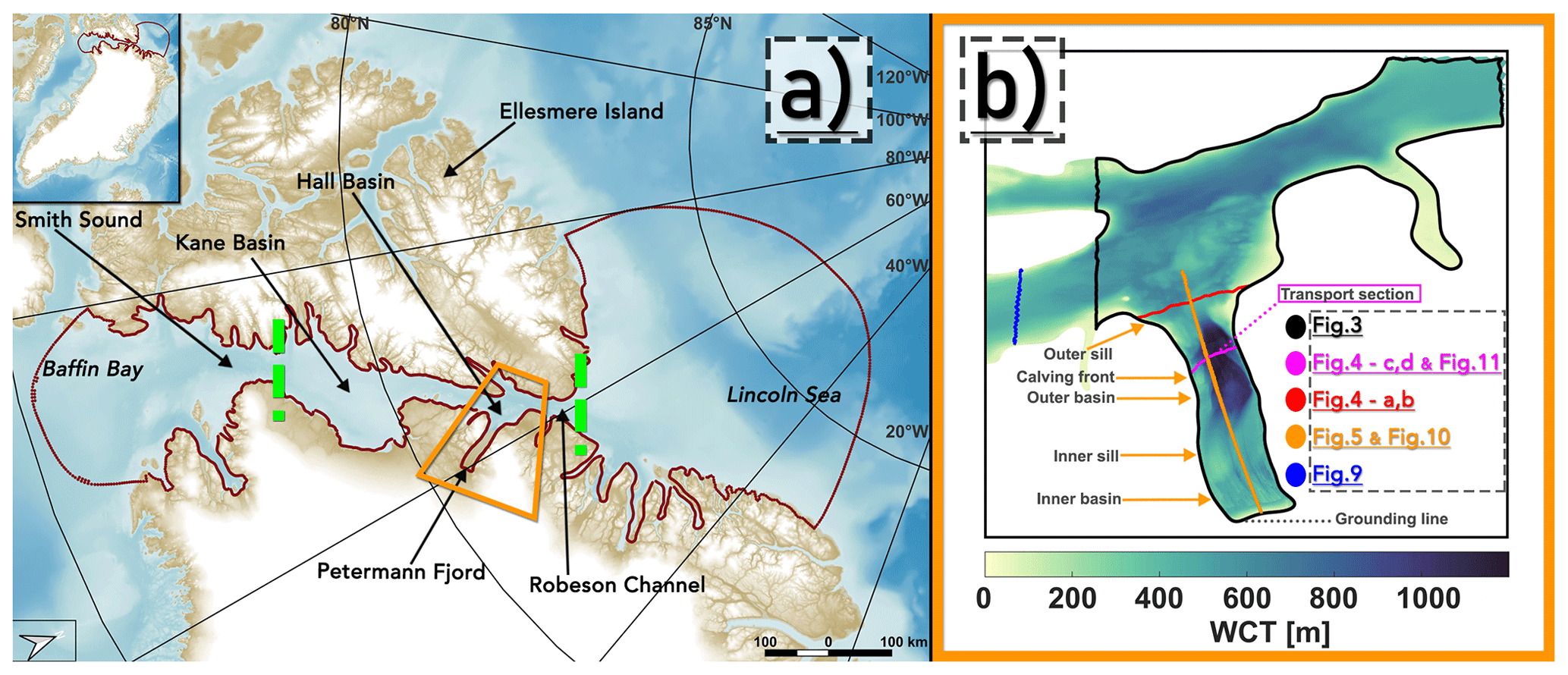
Figure 1Inset in panel (a) shows the location of our regional model domain (outlined in red) on a large-scale map modified from Jakobsson et al. (2020a). A zoomed-in image of the inset shows lateral boundaries defined by the Greenland and Ellesmere Island coastlines, and open ocean boundaries which are located in the Lincoln Sea and Baffin Bay. Dashed green lines mark the approximate locations where the northern (near the Robeson Channel) and southern (between Kane Basin and Smith Sound) sea ice arches usually form. The orange box indicates a subsetted region within which modelled results are presented. Panel (b) is a zoomed-in image of the area within the orange box in panel (a) and shows the model water column thickness (WCT) map. Lines show section locations for which modelled results are presented in Sect. 3 according to the colour-coded legend. Note that the transport section (see Appendix C) is the same as the magenta cross-section.
2.1.3 Model domain, discretization, and topography
The model has been further adapted to render a nested, high-resolution, 3-D ocean–sea ice–ice shelf setup for PGIS and PF. (For a detailed description of the model setup, including selected results from it, see Prakash et al. (2022).) The modelling domain stretches from 75 to 87∘ N and 29 to 81∘ W, covering the PF and Nares Strait with open boundaries located in the Lincoln Sea and Baffin Bay (Fig. 1a). Figure 1b indicates the cross-section locations in PF and adjacent Nares Strait regions at which modelled results are presented in Sect. 3. The horizontal grid is composed of non-overlapping unstructured triangular cells with variable resolution: 200 m in the fjord, 2 km in the near-fjord regions, and 4 km elsewhere. The vertical grid comprises 23 terrain-following σ layers. The fjord bottom topography and the PGIS draft have been derived from BedMachine v3 (Morlighem et al., 2017), wherein the latter represents a period prior to the 2010 calving event. As described in Prakash et al. (2022), the BedMachine v3 dataset has been modified to remedy an inaccurately represented sub-ice-shelf water column thickness and to also include a 540–610 m deep inner sill located ca. 25 km from the GL (Tinto et al., 2015) which is not included in the dataset.
2.2 External forcings
The simulation period spans 1 July 2014 00:00:00 UTC to 1 January 2017 00:00:00 UTC. Model results are presented for the last year (1 January 2016 00:00:00 UTC to 1 January 2017 00:00:00 UTC) as it is closest to the period (2016–2019) which has been characterized by frequent collapse or absence of ice arches, reduced ice flux stoppages, and extraordinarily high ice area flux through the Nares Strait (Moore et al., 2021), and for which we can initialize and run our model using realistic atmosphere, sea ice, and ocean boundary conditions.
2.2.1 Surface forcing
Over the simulation period, we obtain the 3 h surface air pressure, 2 m air temperature, relative humidity, downward longwave radiation, net shortwave radiation, eastward and northward wind speed, precipitation, and evaporation from the polar (p) version of RACMO2.3p2 (Regional Atmospheric Climate Model; Noël et al., 2019). Furthermore, the daily averaged sea ice concentration (Ai) and thickness (hi), bulk ice salinity (Si), and sea ice velocities (Ui) are obtained from the A4 ROMS (4 km pan-Arctic Regional Ocean Modeling System grid) – CICE (Community Ice CodE) run (Hattermann et al., 2016; Hunke et al., 2010). A technical description of the downscaling procedure is provided in Prakash et al. (2022).
2.2.2 Lateral ocean boundary conditions
The FVCOM grid is nested within the A4 ROMS grid, which in conjunction with the 5 km AOTIM (Arctic Ocean Tidal Inverse Model; Padman and Erofeeva, 2004), provides the hourly lateral ocean boundary conditions. Implementation of the nesting procedure has been detailed in Prakash et al. (2022). To alleviate the bias in the upstream A4 temperature and salinity time series (2007–2017), monthly climatologies were constructed from the start of the A4 simulation (2007–2009), when the bias was negligible (see Prakash et al., 2022), and were then interpolated to the hourly forcing intervals. While this procedure resulted in noticeable improvements, the AW in the fjord remained colder and fresher compared with observations (cf. Johnson et al., 2011 and Prakash et al., 2022). To that end, we have implemented a depth-dependent bias correction (as suggested in Prakash et al., 2022) at the boundary such that the modelled temperature and salinity are now consistent with observational data (Johnson et al., 2011) from this period. Lastly, the hourly AOTIM sea surface height (SSH) solution from the simulation period is added to the A4 SSH field from the same period to generate the tidal forcing (see Prakash et al., 2022).
We note that the model in its present configuration does not feature subglacial discharge at the grounding line. While it is known to impact fjord-scale circulation and basal melt rates at Petermann (Cai et al., 2017), the aim of our study is to distinguish the impact of long-term changes in regional sea ice cover on PGIS basal melt. Thus, we posit that the mechanisms identified here in response to a changing sea ice cover, and the associated anomalies (departing systematically from a baseline experiment) in basal melt, are robust regardless of the omission of subglacial discharge. Nonetheless, conjectures regarding its omission on our results are presented in Sect. 4.3.
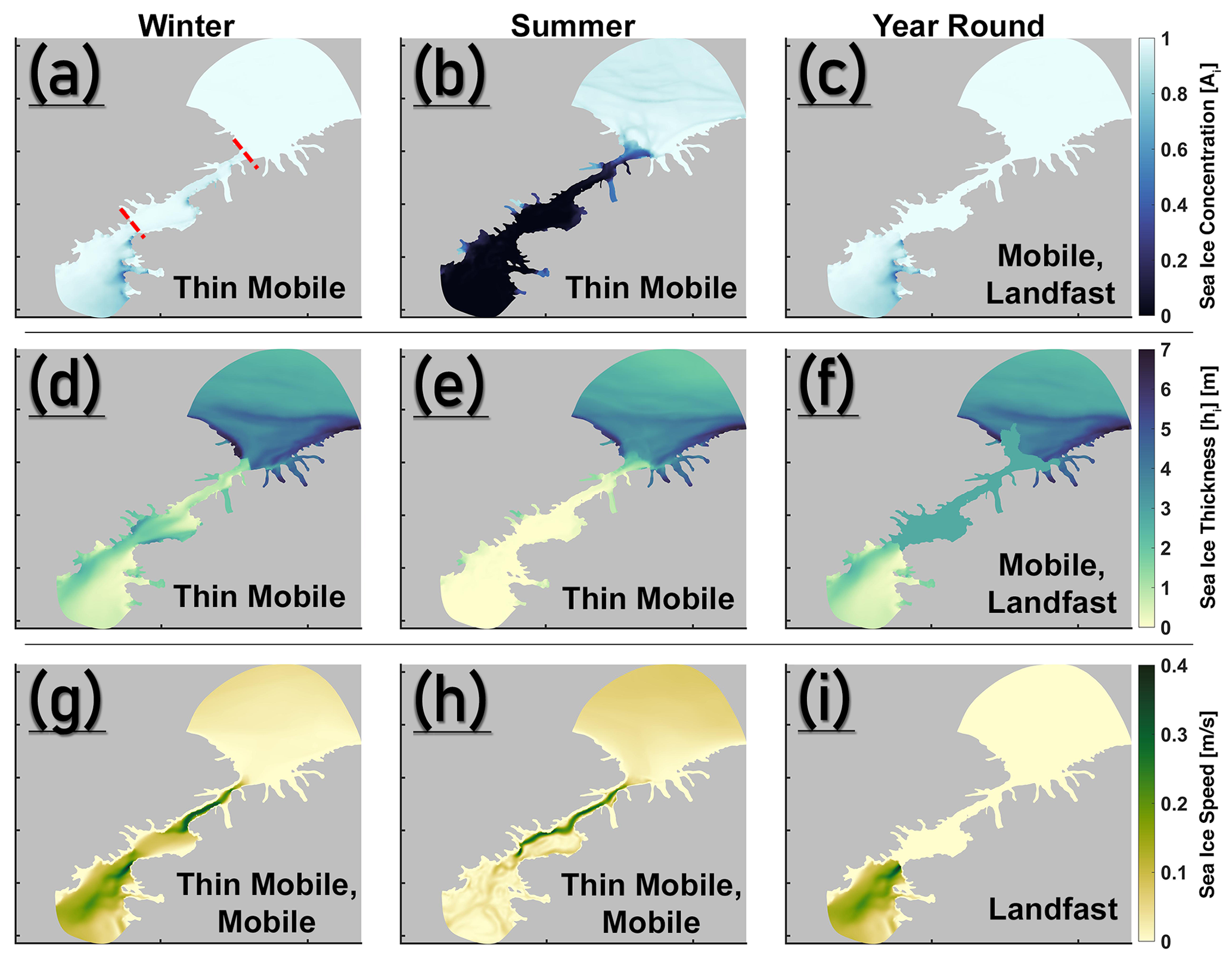
Figure 2Winter (a, d, g), summer (b, e, h), and year-round (c, f, i) sea ice conditions for the Thin Mobile, Mobile, and Landfast experiments. Approximate locations of the northern arch and southern arch are shown as dashed red lines in (a). In each panel, experiment(s) corresponding to the sea ice condition shown are labelled. Note that the Landfast experiment is designed to have zero speed until the southern arch (i), south of which sea ice speeds are similar to those of the Thin Mobile experiment (as an example, winter speeds are shown here).
2.3 Experiment setup
To study the implications of a possible regime shift in sea ice arch formation in the Nares Strait on PGIS basal melt, we conducted three experiments differing only in the applied sea ice forcing (namely Ai, hi, and Ui). These are the Landfast, Mobile, and Thin Mobile experiments. First, we provide a characterization of these regimes, followed by how they are represented in our experiments.
Between 1996 and 2002, landfast sea ice cover prevailed in the Nares Strait for 7–10 months each year following the formation of southern or both northern and southern ice arches (Kwok et al., 2010), which blocked the southward sea ice flux for large parts of the year. In recent years, premature collapse of these arches and an increased failure in arch formation have been reported (Moore and McNeil, 2018; Moore et al., 2021), indicating a shift towards (an extended period of) mobile sea ice cover in the Nares Strait. Additionally, observations evidence that reductions in the Arctic sea ice extent and thickness have persisted over the past two decades and are modelled to continue in the future (Notz and SIMIP Community, 2020; Kacimi and Kwok, 2022). This suggests that a transition towards a year-round thin and mobile sea ice cover is to be expected for the Arctic.
In order to prescribe these regimes as surface forcing to our model, we start with the A4-CICE model output which features a thin and year-round mobile sea ice condition in the Nares Strait (see Sects. 2.2 and 2.2.1 above), facilitated by the absence of an ice arch and mirroring an increasingly often observed (and also a likely standard future) scenario. This is referred to as the Thin Mobile experiment (Fig. 2; Table 1). Thereafter, we modify the Ai, hi, and Ui values of the A4-CICE output from 1 January 2016 to 1 January 2017 to create the Mobile and Landfast experiments (detailed below). The Mobile and Landfast runs are initialized using the stable model solution of the Thin Mobile run on 1 January 2016 00:00:00 UTC (see Appendix B) and are run using modified sea ice forcing until 1 January 2017 00:00:00 UTC.
In the Mobile experiment, we set Ai=1 throughout the year to ensure that the region bounded by the sea ice arches is completely ice covered (Fig. 2; Table 1). This affects seasonality via the removal of open ocean during summer. Additionally, a year-round hi of 2.75 m ensures that the ice cover is sufficiently thick so as to block the heat exchange between the ocean and the local atmosphere. Lastly, (non-zero) Ui is retained from the Thin Mobile experiment. For the Landfast experiment, in addition to the changes made above to design the Mobile experiment, Ui in the Thin Mobile experiment is set to zero throughout the year until the edge of the southern ice arch, which additionally blocks the transfer of momentum onto the ocean (Fig. 2; Table 1). The hi value chosen in the Mobile and Landfast experiments is within the range of sea ice draft values reported in this region (Ryan and Münchow, 2017) and corresponds to the old Arctic multiyear ice advected from the north (of the northern arch) into the Nares Strait, and which is either fastened in place under a landfast regime or carried further southward following the absence or collapse of an ice arch. Also, estimates of ice flux stoppage duration, particularly from the 1998–2001 period, justifies our imposition of a fast ice cover over both the winter and summer seasons (Kwok et al., 2010). Therefore, the Landfast experiment and the contrasting results presented with respect to it in the Mobile and Thin Mobile experiments are plausible.
Table 1Numerical experiment characteristics. Winter and summer seasons correspond to days 30–105 and 170–245 of the 2016 calendar year.
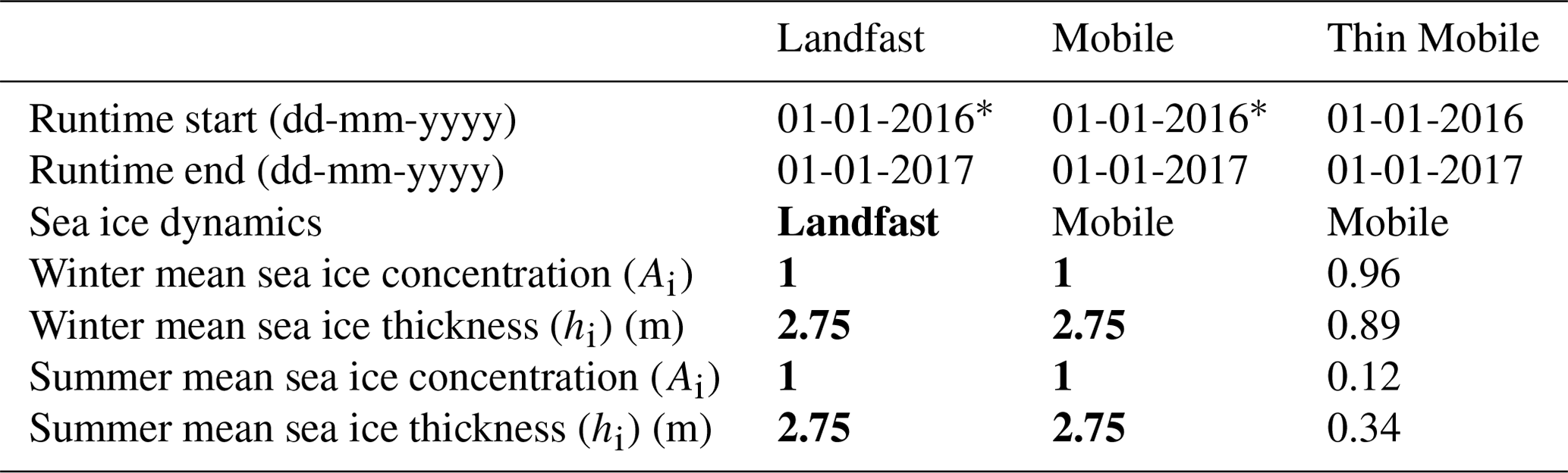
* The Landfast and Mobile runs are initialized using the stable model solution of the Thin Mobile run on 1 January 2016 00:00:00 UTC and are run using modified sea ice conditions. Modifications in the sea ice conditions in the Landfast and Mobile experiments with respect to the Thin Mobile experiment are highlighted in bold. Ai and hi values represent the seasonal mean sea ice conditions in the Nares Strait region bounded by the sea ice arches (Fig. 2(a)).
Below, the seasonal mean ocean circulation and fjord water mass characteristics are described first for the Landfast experiment. The drivers of melt, namely friction velocity (u*) and thermal driving (ΔT), are analysed and their contributions to PGIS basal melt are presented (Sect. 3.1.1, 3.1.2, and 3.1.3). Thereafter, these results are compared with the Mobile and Thin Mobile experiments in order to discern the seasonal thermo-mechanical impact of sea ice concentration, thickness, and mobility on the ocean circulation and PGIS basal melt (Sect. 3.2.1, 3.2.2, and 3.2.3).
3.1 Landfast experiment
3.1.1 Depth averaged seasonal mean currents
The depth- and seasonally (Table 1) averaged circulation in the wider PF area, which includes PF as well as the Hall Basin and Robeson Channel in the Nares Strait, is shown in Fig. 3a and b. In summer, a general southward current is observed in the Nares Strait which has a cross-strait component in the Hall Basin region; however, the circulation in winter appears more complex because of several flow reversals in the Robeson Channel and the Hall Basin region. Mean speeds during winter are generally lower than during summer, when speeds attain their highest values along the Canadian Nares Strait coast. Near the mouth of PF, irrespective of the season, the circulation is characterized by lateral inflow and outflow supported by the western and eastern coastal boundaries, respectively (further discussed in Sect. 4.1). Moreover, a cyclonic (counter-clockwise) gyre enables exchange between the PF and Hall Basin (further discussed in Sect. 4.1). Underneath the deeper regions of the ice shelf draft, close to the GL, a similar cyclonic circulation pattern is formed, seaward of which an anticyclonic flow resides over the inner-sill region (Fig. 3).
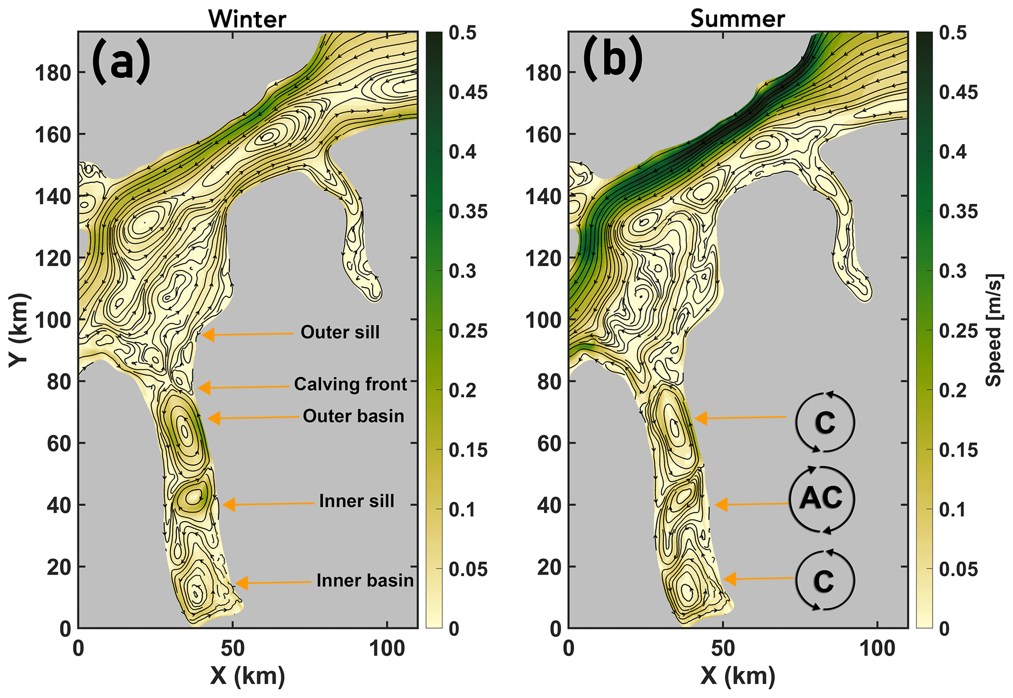
Figure 3Depth averaged seasonal mean speed of the modelled ocean velocities for (a) winter and (b) summer with mean streamlines overlaid for the area indicated in Fig. 1b. Selected topographic features in PF are labelled in (a). Location of the cyclonic (C) and anticyclonic (AC) gyres in PF are shown in (b). Note that the streamlines were generated using the “streamslice” function on Matlab and, as such, are not well-defined conservative stream functions but are used to assist in visualizing the circulation patterns.
3.1.2 Seasonal mean normal flow across the outer sill and into the PGIS cavity
Across the mouth of the PF and PGIS (see Fig. 1b), the seasonal mean normal flows to them are shown in Fig. 4, overlaid with corresponding isotherms and isopycnals. Near the fjord mouth, mean velocity attains magnitudes of ca. 0.1 m s−1 (Fig. 4a, b). Inflow (positive normal velocities) and outflow (negative normal velocities) in winter are largely confined to the western and eastern fjord sector, respectively. In summer, a strong subsidiary outflow is seen in the 50–250 m depth range close to the western flank (further discussed in Sect. 4.2). In winter, we find 0 ∘C (σ0=27.9 kg m−3, where σ0 is the potential density anomaly referenced to 0 dbar) water spilling over the outer sill into the outer fjord basin (Fig. 4a), whereas in summer the overflowing AW are relatively warmer and denser (Fig. 4b).
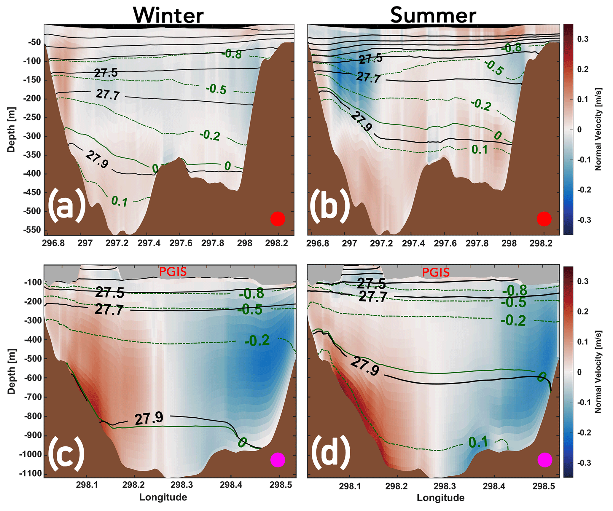
Figure 4Winter (a, c) and summer (b, d) mean normal velocity with mean isotherms (green stippled lines, green label) and mean isopycnals (black solid line, black labels) overlaid. Isotherms are plotted at equally spaced intervals of 0.3 ∘C and isopycnals are plotted at equally spaced intervals of 0.2 kg m−3. The 0 ∘C isotherm is shown by a green solid line. Positive values are directed towards the GL. The colour-coded circle within each panel indicates the location of the cross-section; see Fig. 1b.
Near the PGIS calving front, irrespective of the season, inflow and outflow remain largely confined to the western and eastern regions of the fjord, respectively (Fig. 4c, d). In winter, inflow into the PGIS cavity of up to ca. 0.15 m s−1 is modelled, whereas, in summer it is seen to intensify with depth (600–1050 m) with velocities reaching up to ca. 0.35 m s−1 (further discussed in Sect. 4.2). We find the 0 ∘C isotherm and the 27.9 kg m−3 isopycnal surface near the bottom of the outer basin (ca. 900 m depth) during winter (Fig. 4(c)), whereas in summer they are lifted above the GL depth of ca. 600 m (Fig. 4d). As we will show in Sect. 3.1.3, in summer, 0.1 ∘C (σ0=27.9 kg m−3) warm AW fills the greater depths of the inner fjord basin and comes into contact with the GL. These results indicate a larger admixture of AW into the cavity during summer.
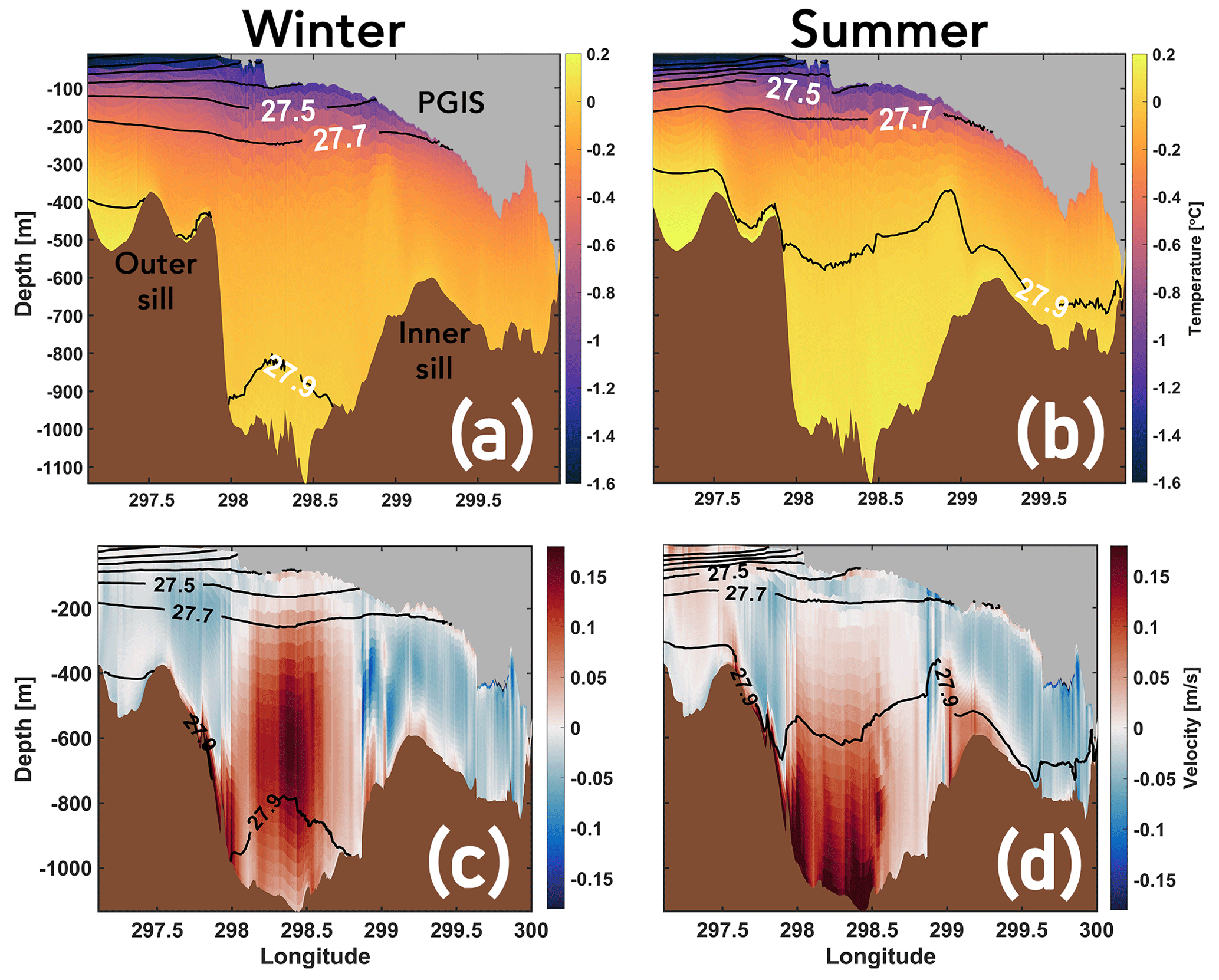
Figure 5Seasonal mean temperature (a, b) and flow (c, d) along the fjord with mean isopycnals (black solid lines) overlaid; see Fig. 1b for section location. The GL is to the right in each panel. Isopycnals are plotted at equally spaced intervals of 0.2 kg m−3. In (c) and (d), positive values correspond to inflow into the fjord.
3.1.3 Oceanic controls on PGIS basal melt for the Landfast experiment
Modelled winter and summer mean temperatures (Fig. 5a, b) and along-fjord flow (Fig. 5c, d) overlaid with corresponding mean isopycnals (plotted at equal intervals of 0.2 kg m−3) are shown for a transect (see Fig. 1b) stretching from the fjord mouth (left margin) to the GL (right margin). In both seasons, the cold and fresh polar water (PW), largely characterized by surface processes, occupies the upper ocean layer (depth 50–100 m) of PF (Fig. 5a, b). A strong pycnocline separates this PW layer (σ0<27.3 kg m−3; and which does not subduct below PGIS draft >100 m) from the underlying water column. The AW layer seaward of the outer sill is found at greater depths (>200 m; σ0>27.7 kg m−3). The 27.9 kg m−3 isopycnal surface represents the warm and dense AW from Hall Basin that overflows from the outer sill and enters PF. In winter, we do not evidence this surface crossing the inner sill, and it is restricted to the greater depths of the outer fjord basin (Fig. 5a). The warmest AW is modelled to be between 0 and 0.1 ∘C in the outer fjord basin, and between −0.1 and 0 ∘C in the inner fjord basin. In summer, however, the isopycnals are lifted up, allowing the 27.9 kg m−3 surface to cross the inner sill and contact the GL (Fig. 5b). Thus, in summer a relatively warmer and denser AW fills the outer and inner fjord basin compared with winter. We locate the warmest AW between 0.1 and 0.2 ∘C in the outer basin, and between 0 and 0.1 ∘C in the inner basin. The presence of a ca. 0.1 ∘C warmer AW in the inner basin in summer is likely to increase basal melting, thus strengthening the melt-driven fjord-scale overturning (i.e. buoyancy) circulation (Fig. 5c, d). Here, a stronger outflow of the buoyant meltwater plume rising along the PGIS base is matched by a stronger inflow of AW at a depth which extends deeper into the inner basin, thus entraining more AW in the interior of the PGIS cavity. The glacially modified water deposited by the plume is seen to occupy the intermediate (100–200 m) depths bounded by the 27.3 and 27.7 kg m−3 isopycnals. As we will show below, a contrasting response of PGIS basal melt is modelled for water columns above and below the 27.7 kg m−3 isopycnal surface (i.e. PGIS draft less than or greater than 200 m) driven by seasonal changes in melt-driven overturning circulation in the fjord.
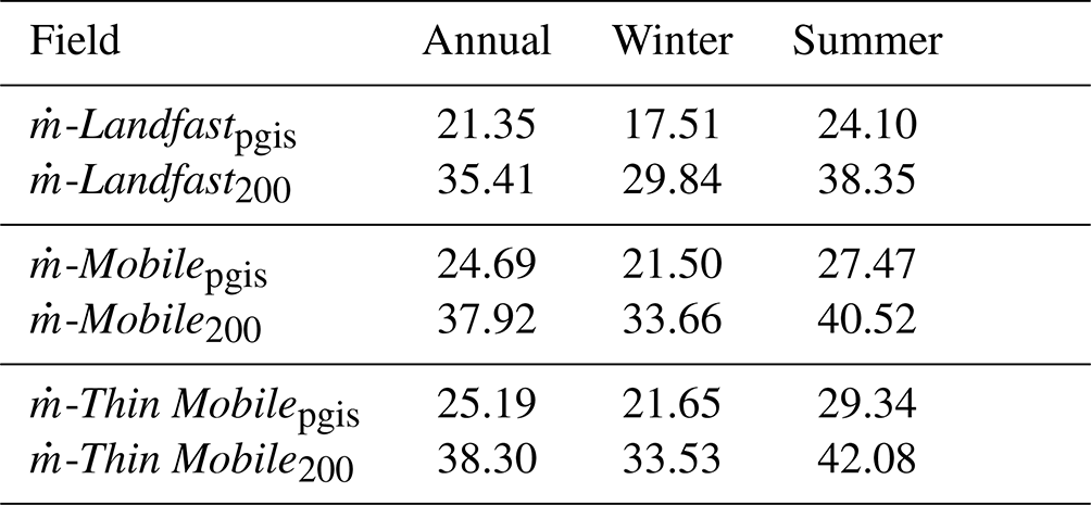
The winter and summer mean, and the changes in summer relative to winter, are shown for the modelled PGIS basal melt rates and its drivers, namely thermal driving (ΔT) and friction velocity (u*) (Fig. 6). We find that irrespective of the season, mean melt rates show strong spatial variability, largely ranging from a few metres per year up to 80–100 m yr−1 (Fig. 6a, b). The strongest melting occurs towards the eastern sector of the ice shelf slightly north of the GL, and gradually decreases downstream. Regions exhibiting more melting are aligned with the ice flow direction. Summer mean melt rates are considerably higher than winter nearly throughout the domain (Fig. 6c). Here, increases of up to 20–30 m yr−1 are modelled in regions further downstream of the GL, seaward of which, however, we note nominal decreases of up to ca. 5 m yr−1 towards the western fjord sector near the PGIS calving front. The annual mean modelled melt rate averaged over the entire PGIS base is calculated as 21.35 m yr−1, with winter and summer mean modelled melt rates being 17.51 and 24.10 m yr−1, respectively (see Table E1).
We note that the PGIS geometry exerts a strong control on the modelled mean basal melt rates: higher melt is seen for regions characterized by deeper ice shelf drafts and/or steeper ice shelf basal slopes, and is consistent with the spatial variability seen in the satellite derived estimates reported by Wilson et al. (2017). Sub-ice-shelf channels resulting from channelized basal melting of PGIS (Rignot and Steffen, 2008) have imposed steep transverse and longitudinal ice shelf draft gradients. These channels are several kilometres wide and extend along the length of PGIS, deepening in the direction of the ice flow. A steeper PGIS basal slope supports stronger entrainment in the buoyant meltwater plumes. Under the deeper (400–600 m) drafts, the seawater melting point is considerably lowered. Near the GL, and particularly towards the eastern sector of the ice shelf, PGIS draft is deepest and also features some of the steepest slopes.
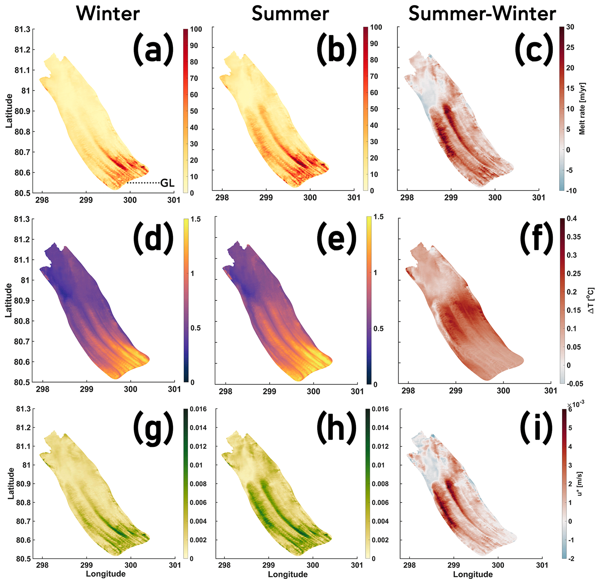
Figure 6Seasonal mean modelled melt rate (a–c), thermal driving (ΔT) (d–f), and friction velocity (u*) (g–i) at the base of PGIS for winter (a, d, g), summer (b, e, h), and the increase in summer with respect to winter (c, f, i) for the Landfast experiment. The “GL” label in (a) indicates the location of the grounding line.
In winter, we see higher ΔT (1–1.4 ∘C) near the GL as compared with regions seaward of it (Fig. 6(d)). A higher local melt (Fig. 6a) generates a strong outflow plume which increases the u* slightly downstream of the GL (Fig. 6g). Although ΔT is more pronounced along the eastern flank near the GL, it is evident that melt rate maxima occur slightly downstream where u* peaks (0.012–0.014 m s−1) (cf. Fig. 6a, d, g). Thus, the variability in melt is congruent with that of u*. This also holds true for summer (cf. Fig. 6b, e, h), however, with notable differences that reflect the seasonal changes in ocean properties. Here, compared with winter, an increase in ΔT near the GL (ca. 0.1 ∘C) drives an increased melt, and thus, a more vigorous outflow plume which further strengthens the u*, with most noticeable differences (0.004–0.006 m s−1) modelled further downstream of the GL (Fig. 6c, f, i). Strengthening of u* here is seen to enhance ΔT (0.25–0.3 ∘C) by increasing the friction-driven turbulent mixing which brings more heat from the interior ocean to the PGIS base (see Gwyther et al., 2015; Zhou and Hattermann, 2020). Furthermore, the increased meltwater production and stronger melt-driven overturning also brings more cold meltwater from depth towards the calving front which leads to a decrease in ΔT, and thus melt, beneath the shallow ice shelf base. These seasonal patterns are qualitatively similar across all experiments (not shown here), with differences that arise due to changes in sea ice cover investigated in Sect. 3.2.
3.2 Response of PGIS basal melt to climate-warming-driven changes in sea ice cover
3.2.1 Amplification of PGIS basal melt
To illustrate the amplification of PGIS basal melt in response to the sea ice cover transitioning from Landfast to Mobile and Thin Mobile, annual and seasonal mean melt rate anomalies for the Mobile and Thin Mobile runs with respect to the Landfast run are shown in Fig. 7. We calculate an increase in the ice shelf averaged annual mean modelled basal melt rate of 3.34 m yr−1 in the absence of a landfast sea ice cover, and an additional increase of 0.50 m yr−1, as the sea ice regime, in addition to being mobile, becomes thin (Fig. 7a, d, g). During winter, a transition from Landfast to Mobile yields a 3.99 m yr−1 increase in mean melt, whereas in summer this increase is 3.37 m yr−1 (Fig. 7b, c, e, f). Additionally, as the sea ice cover thins, a further increase in winter and summer mean melt rates of 0.15 and 1.87 m yr−1, respectively, is modelled (Fig. 7b, c, h, i). Thus, a net increase, driven by a transition from Landfast to Thin Mobile, of 18 % is modelled annually, with corresponding winter and summer increases of 24 % and 22 %, respectively (For further discussion, see Sect. 4.5; also see Table E1.)
Changes in ΔT and u* are used to investigate the drivers of these changes in basal melt (Fig. 8). Here, the shallower (<200 m) and deeper (>200 m) regions of PGIS exhibit a contrasting response. Under the deeper drafts, increase in ΔT is negligible; however, u* increases considerably and is congruent with the melt rate increase. This implies that any noticeable increase in melt in this region is solely driven by a more energetic circulation through increased vertical current shear. Although, unlike the annual and winter mean, the summer mean ΔT shows a nominal increase of ca. 0.025 ∘C (cf. Fig. 8d, e, f). This implies that the increase in melt during summer also entails contribution from ΔT (further discussed in Sects. 3.2.2 and 3.2.3). Increases in annual and seasonal mean modelled melt for the shallower drafts are driven by increases in both ΔT and u* (further discussed in Sects. 3.2.2 and 3.2.3) (Fig. 8). For the Thin Mobile run, the additional increase in summer mean melt of shallower ice compared with that of the Mobile run is due to the heat gained by the upper (open) ocean from the atmosphere. However, it is noteworthy that any increases in u* could also contribute towards increases in ΔT seen in these scenarios (as discussed in Sect. 3.1.3).
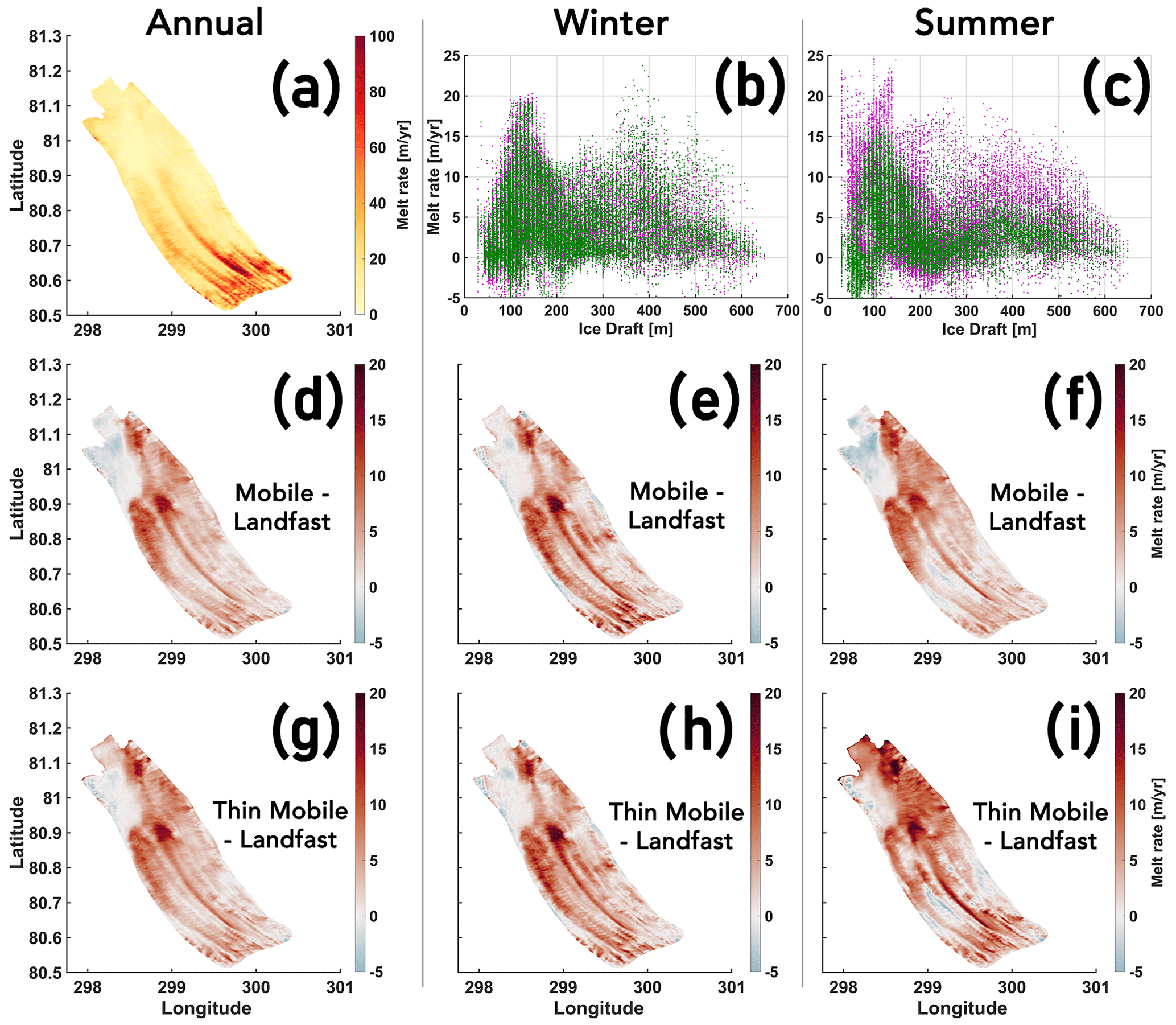
Figure 7PGIS annual modelled mean melt rate for the Landfast experiment (a), with Mobile (d) and Thin Mobile (g) anomalies shown relative to it. Winter (b, e, h) and summer (c, f, i) modelled mean melt rate anomalies for the Mobile and Thin Mobile experiments are shown relative to the Landfast experiment; plotted vs. the ice draft (b, c) and as 2-D anomaly maps under the PGIS base (e, f, h, i). Colour coding for (b) and (c): Mobile – Landfast = green, and Thin Mobile – Landfast = purple.
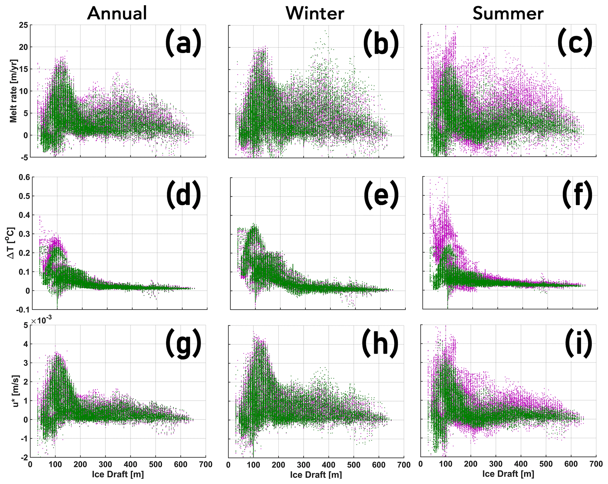
Figure 8The Mobile and Thin Mobile melt rate (a–c), thermal driving (ΔT) (d–f), and friction velocity (u*) (g–i) anomalies are shown relative to the Landfast experiment. Panels (a, d, g), (b, e, h), and (c, f, i) correspond, respectively, to the annual, winter, and summer means. Colour coding for all panels: Mobile – Landfast = green, and Thin Mobile – Landfast = purple.
3.2.2 Changes in far field water mass properties
Changes in ocean circulation in the Nares Strait in response to the perturbed surface forcing influences conditions in PF, which partly contributes to the changes in ΔT and u* discussed above (Sect. 3.2.1). When the sea ice cover transitions from Landfast to Mobile (Fig. 9a, b), a southward wind-driven surface current in the Nares Strait causes a westward Ekman transport (consistent with findings reported in Shroyer et al., 2017; see further discussion in Sect. 4.4), wherein the cold and fresh surface PW being displaced towards the Ellesmere Island (west) coast are replaced by the warm and saline AW at depths that are pulled up towards the Greenland (east) coast. Increase in salinity between 0.2 and 0.45 psu (practical salinity units) are modelled in the upper 150 m of the water column along the Greenland coastline (Fig. 9a, b).
When the sea ice cover, in addition to being mobile, becomes (negligibly) thin, latent heat loss resulting from strong atmospheric cooling during winter in the high Arctic over open ocean/thin ice supports a period of enhanced local sea ice production. Brine rejected during sea ice formation results in salinification of the upper ocean layer (i.e. first σ layer). The resulting loss of stratification destabilizes the water column and drives a thermohaline convection which allows further upwelling of the deeper-lying AW (Fig. 9c, e, f). An increase in salinity of up to ca. 0.05 psu is modelled in the upper 150 m of the water column along the Greenland coastline. At the onset of summer, owing to a warmer atmosphere, cessation of sea ice formation is seen (Fig. 9e). Furthermore, the heat gain drives enhanced sea ice melting resulting in significant freshening of near surface waters (Figs. 9d, D1). These changes are communicated to the fjord (see Fig. 3; further discussed in Sect. 4.1) where similar changes in seasonal mean salinity (isopycnals) are noted (discussed further in Sect. 3.2.3).
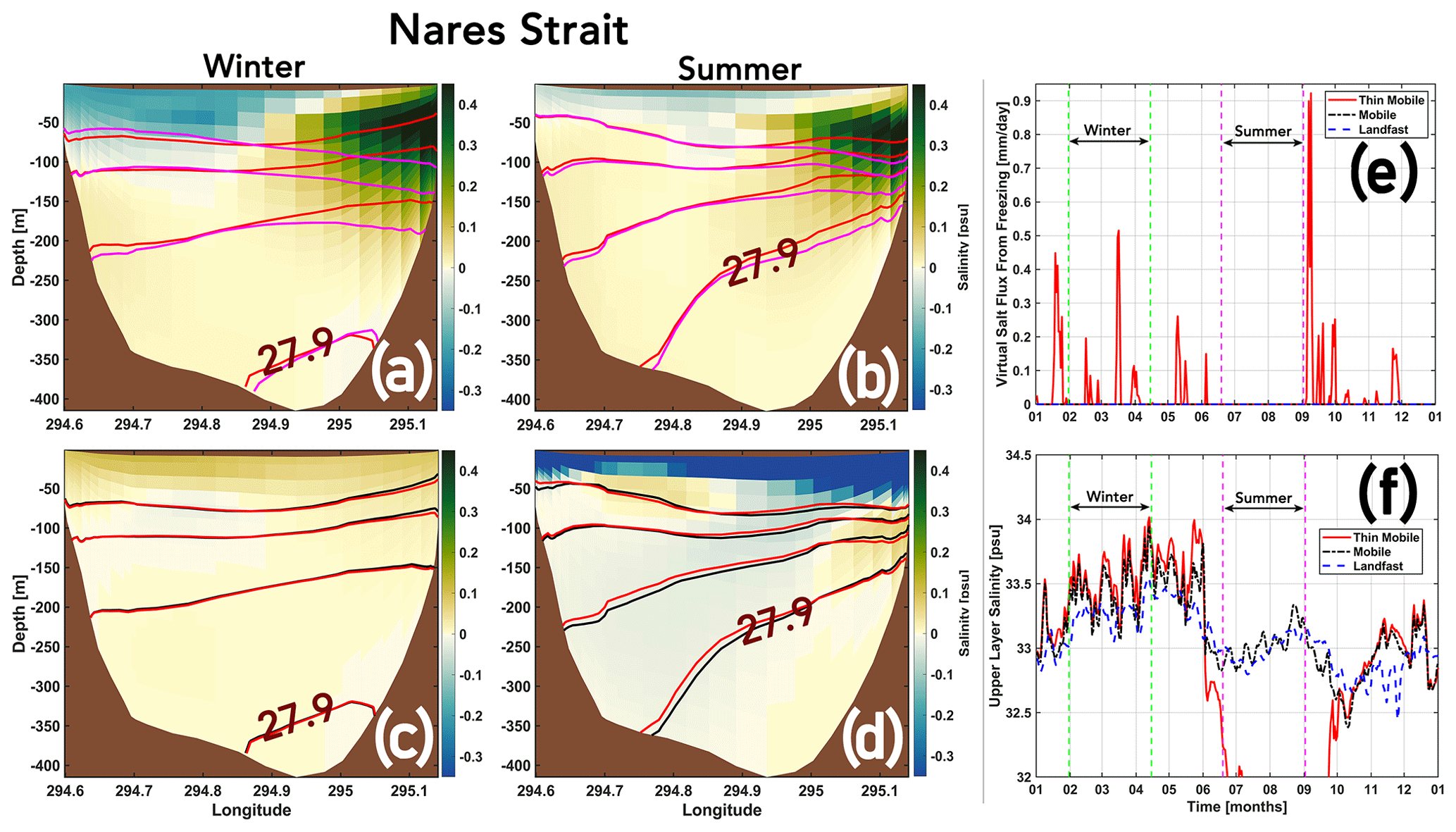
Figure 9Seasonal mean modelled changes in salinity for the Mobile – Landfast (a, b) and Thin Mobile – Mobile (c, d) experiments, across a section in the Nares Strait, south of PF (see Fig. 1b for location). Isopycnals are plotted at equally spaced intervals of 0.2 kg m−3, where magenta, red, and black represent the seasonal mean values for the Landfast, Mobile, and Thin Mobile experiments, respectively. Time series (2016) of the virtual salt flux due to sea ice freezing (e) and the upper layer salinity (f) for the three experiments are shown for a node on the Nares Strait section near the eastern (Greenland) coastline. The stippled green and magenta lines in (e) and (f) indicate the span of the winter and summer seasons, respectively.
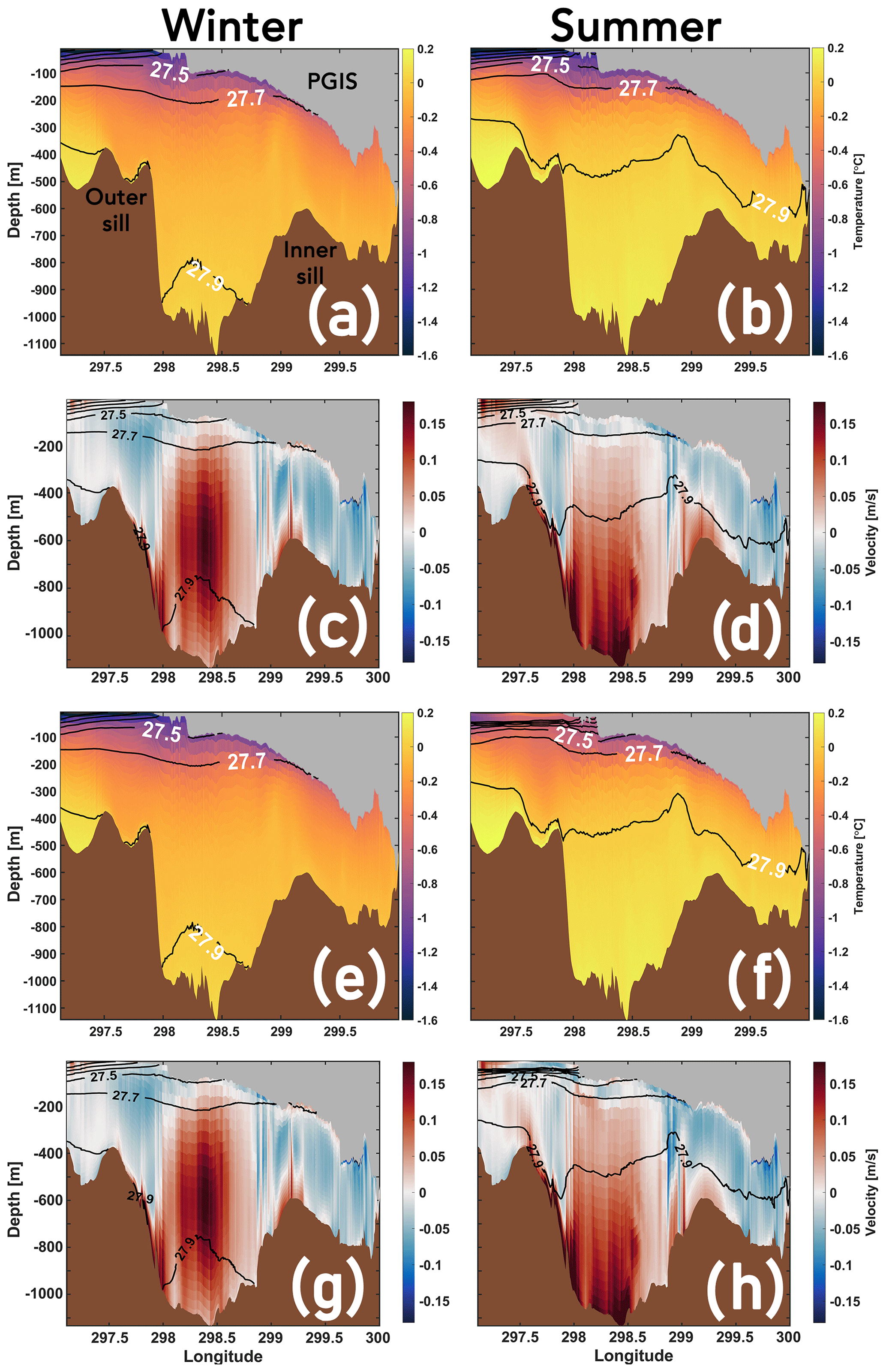
Figure 10Seasonal mean temperature (a, b, e, f) and flow (c, d, g, h) along the fjord with mean isopycnals (black solid lines) overlaid; see Fig. 1b for section location. GL is to the right in each panel. Panels (a–d) and (e–h) represent the Mobile and Thin Mobile experiments, respectively. Isopycnals are plotted at equally spaced intervals of 0.2 kg m−3. Positive flow values correspond to inflow and are directed towards the GL.
3.2.3 Changes in oceanic conditions in the fjord
Increases in heat and salt content, and the circulation in the PGIS cavity in response to climate warming induced long-term changes in sea ice cover, drives enhanced basal melt. To study these changes in the oceanic conditions in the fjord, seasonal mean temperature and flow along the fjord are shown in Fig. 10 (section is same as Fig. 5 and shown in Fig. 1b) for the Mobile and Thin Mobile experiments, with corresponding mean isopycnals overlaid. To complement these diagnostics, changes in the seasonal mean normal flow directed into the PGIS cavity are shown in Fig. 11 as the sea ice cover transitions from Landfast to Mobile to Thin Mobile (section is same as Fig. 4c, d and shown in Fig. 1b).
During both winter and summer, as the sea ice cover transitions from Landfast to Mobile, the wind upwelled warm and saline AW from the Nares Strait (Sect. 3.2.2) enter the ice shelf cavity, resulting in an increase in temperature and salinity (cf. Figs. 5a, b and 10a, b). Increases in winter (up to ca. 0.25 ∘C, 0.2–0.25 psu) are relatively higher compared with summer (up to ca. 0.15 ∘C, 0.1–0.15 psu); however, they are largely confined to the shallower (<200 m) drafts (Fig. D2a, b, c, d). Thus, as compared with the Landfast run, a distinct shift is seen in the density of the upper ca. 200 m of the water column in winter, wherein the isopycnal surfaces represented by σ0≤27.7 kg m−3 are lifted up (cf. Figs. 5a, 10a). In particular, we note that the layer bounded between kg m−3 is broadened such that PGIS drafts between 100 and 200 m are now contacted by relatively denser waters. On the other hand, in summer this shift is further exacerbated and includes the dense 27.9 kg m−3 AW surface that is lifted further above the inner sill depth (cf. Figs. 5b, 10b). Additional increases in subsurface temperature and salinity are seen as we transition further to a Thin Mobile sea ice cover (Fig. 10e, f). In winter, these nominal increases of up to ca. 0.02 ∘C and 0.02 psu correspond to the convectively overturned AW (Sect. 3.2.2) (Fig. D2e, g); however, we do not notice any discernible change in the isopycnals (cf. Fig. 10a, e). In summer, the shortwave heated near surface waters that are 0.1–0.3 ∘C warmer are seen to encroach under the shallower (outer) regions of the ice shelf base (Fig. D2f), and at depth, nominal increases of ca. 0.02 ∘C and 0.02 psu are noted (Fig. D2f, h), accompanied by a nominal, yet notable, lifting of the 27.9 kg m−3 isopycnal surface (discussed further below) (cf. Fig. 10b, f).
Under a mobile sea ice cover, we note a strengthening of the seasonal mean fjord-scale overturning circulation as compared with the landfast scenario. Inflow of a warmer and denser AW intensifies, confined to the western fjord sector (Fig. 11a, b) and extending deeper into the interior of the PGIS cavity (cf. Figs. 5c, d and 10c, d). The largest increments (0.03–0.04 m s−1) are modelled near the ice shelf base in the 100–300 m depth in winter, whereas in summer those are found further near the bottom (400–600 m) (Fig. 11a, b). Furthermore, (meltwater) outflow rising along the PGIS–ocean boundary is notably stronger during both seasons (cf. Figs. 5c, d and 10c, d; also see Fig. D3a, b). Under a mobile and thin sea ice cover, during winter, nominal increases are noted in the inflow and outflow as compared with the mobile ice cover (cf. Fig. 10c, g; see also Figs. 11 and D3). Increases of up to ca. 0.01 m s−1 in the inflow (Fig. 11c) and outflow (Fig. D3c) are largely confined to the layers adjacent to the PGIS base along the western and eastern fjord sectors, respectively. During summer, a considerable strengthening of the overturning circulation is seen (cf. Fig. 10d, h). Substantially higher inflow increases of 0.03–0.1 m s−1 extending to depths of ca. 1000 m are modelled (Fig. 11d), along with a stronger outflow of the buoyant meltwater plume (cf. Fig. 10d, h; see also Fig. D3d).
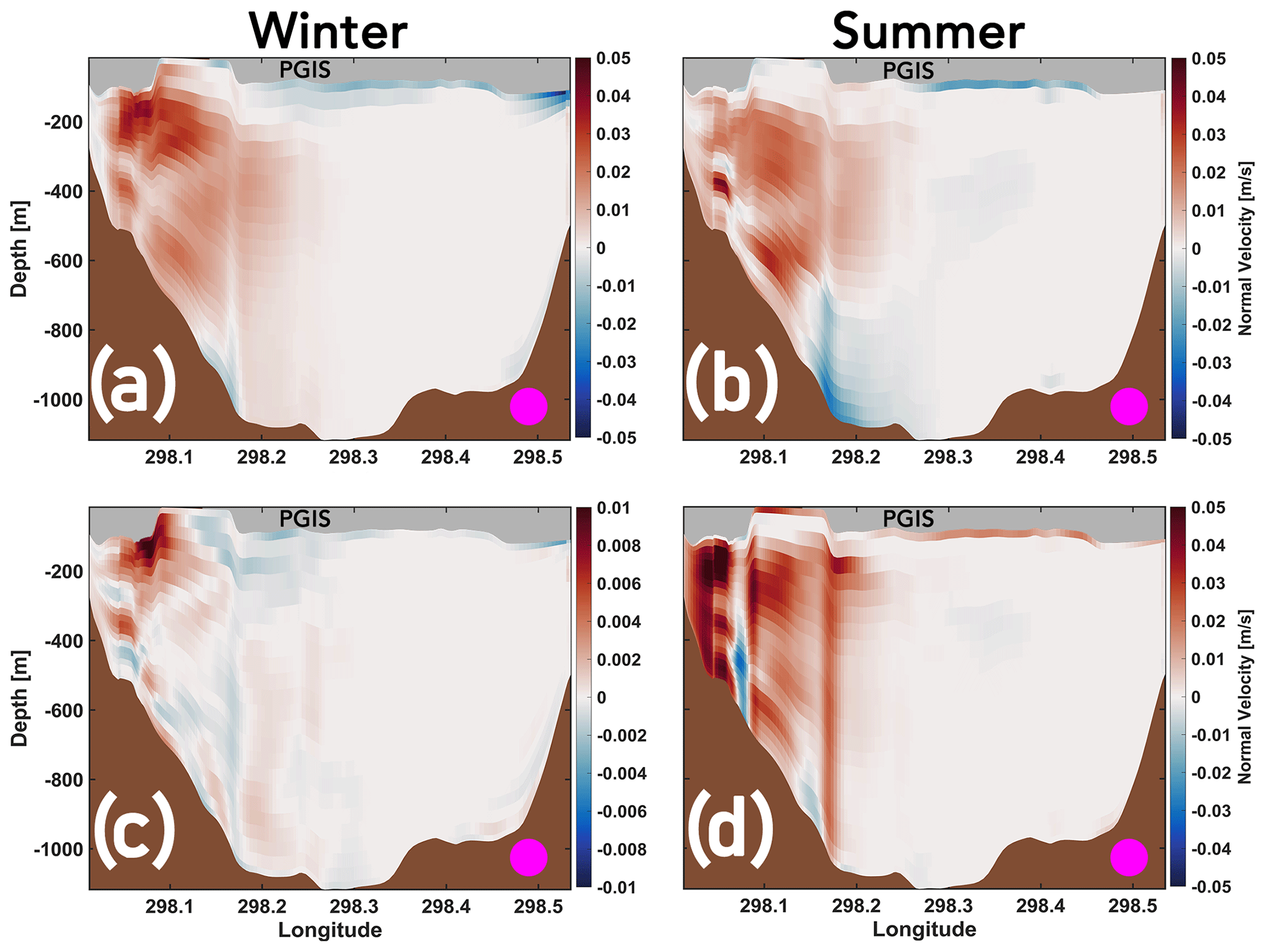
Figure 11Mobile – Landfast (a, b) and Thin Mobile – Mobile (c, d) seasonal mean inflow anomalies across the PGIS section (represented by magenta circles) shown in Fig. 1b. Positive values correspond to strengthening of inflow into the PGIS cavity, whereas negative values correspond to its weakening (and not an outflow), as detailed in Appendix C. Note the different scale used in (c). The corresponding diagnostic for flow directed out of the fjord is presented in Fig. D3.
In summary, during winter, while there is an increase in temperature in PF driven by far field changes for drafts >200 m, this is negligible compared with the changes seen under the shallower (<200 m) drafts (Fig. D2a, e). Evidently, an unperturbed ΔT for drafts >200 m (Fig. 8e) suggests that any increase in melt (Fig. 8b), and thus, the melt-driven fjord-scale overturning circulation, must come from other sources. A congruent increase in u* and melt is noted (Fig. 8b, h), evidencing that increased melting is controlled solely by a stronger boundary layer current. We posit that the strengthening of the circulation (cf. Figs. 5 and 10; also see Figs. 11 and D3) is likely a result of an increased transfer of mechanical energy from air to sea as the sea ice becomes mobile and thin (further discussed in Sect. 4.5). Indeed, the resulting increased melt will drive a stronger melt overturning which would likely act in concert with the mechanically enhanced circulation to amplify u* (and ΔT) downstream of the GL (as discussed in Sect. 3.1.3), and thus, the basal melt. During summer, for drafts >200 m, the increased temperature in the cavity (Fig. D2b, f) plays a role in increasing melt via ΔT (Fig. 8c, f), which contributes towards the strengthening of the melt overturning. However, when transitioning from a Mobile to a Thin Mobile sea ice cover, we note that a negligible increase in ΔT (Fig. 8f) juxtaposed against a substantial increase in u* (Fig. 8i) further suggests that a likely increased air–sea momentum flux over vast areas of open ocean and/or negligibly thin sea ice strengthens the circulation, which predominantly drives basal melting under the deeper drafts (Fig. 8c, i).
4.1 Topographic control on the mean circulation in the fjord
The modelled mean flow in summer from the Hall Basin and north of the PGIS calving front is consistent with remotely sensed summer snapshots of the surface circulation from this region (Johnson et al., 2011), which provided evidence of a general southward current in the Nares Strait, with a cross-strait component in the Hall Basin. Furthermore, the presence of a similar (cyclonic) gyre was noted in the remotely sensed snapshot near the mouth of PF and was also modelled by Shroyer et al. (2017) under a summer mobile sea ice cover. Near the fjord mouth, the lateral inflow along the western fjord wall is directed equatorward, whereas the outflow along the eastern fjord wall is directed poleward (Fig. 3). This resembles a Kelvin wave propagation and is in agreement with the modelled findings reported by Shroyer et al. (2017). In Fig. 3, streamlines have only been presented for the Landfast experiment. Counterparts for the Mobile and Thin Mobile experiments are presented in Fig. D4. Our results evidence that bathymetry exerts a major control on the mean circulation prevailing in PF (cf. Figs. 3 and D4), as the modelled circulation patterns are relatively similar across the three experiments and persist irrespective of season; yet, they vary in magnitude in response to modulations in the buoyancy forcing and changes in surface boundary conditions induced by regional sea ice cover changes (further discussed in Sect. 4.5). Thus, given the influence of topography on the mean circulation in the fjord, we suggest that the exchange of water masses between the Nares Strait and the PF is maintained all year round which facilitates the renewal of water masses in the fjord. Furthermore, the warm and saline AW that enter the PF at depth are effectively circulated in the PGIS cavity and transported to the GL. However, we note that since the circulation is additionally modulated by factors such as buoyancy (including subglacial discharge, which is not included in this study), which is amplified in summer compared with winter, the renewal times are likely to be lower in summer as compared with winter (Carroll et al., 2017; Hager et al., 2022).
4.2 Characteristics of seasonal mean normal flow in the fjord
Under a Landfast sea ice cover in the Nares Strait, strengthening of the inflow of the warmer and denser AW into the PGIS cavity during summer as compared with winter (see Figs. 4 and 5) is caused by a stronger melt-driven overturning circulation (Fig. 6). Previous studies on other high-silled glacial fjords of Greenland have highlighted the role of buoyancy in forcing fjord-scale circulation and driving seasonality (Straneo and Cenedese, 2015; Hager et al., 2022; Kajanto et al., 2023). The stronger summer inflow events, in turn, deliver larger volumes of warmer AW deep into the PGIS cavity.
In PF, this inflow is bottom intensified and the outflow has an ancillary component higher up in the water column (depth <250 m) along the western flank (Fig. 4). Such strong bottom-intensified slope currents have been noted for other large Greenland fjords which feature a similar geometry. For example, at Kangerdlugssuaq Fjord in southeast Greenland, Fraser et al. (2018) modelled weak mean flows at the mouth of the fjord, which intensified with depth, exhibiting current cores of ca. 0.15 m s−1 concentred at the fjord walls around the 400–600 m depth range. Furthermore, summer snapshots acquired during hydrographic surveys in the PF region provided evidence of a thick layer of PGIS meltwater located in the 50–300 m depth range (Johnson et al., 2011; Heuzé et al., 2017). This meltwater layer was reported to be bounded by cold and fresh polar surface waters above, and warm and dense AW below, as well as to leave PF along its eastern sector. However, rich concentrations of PGIS meltwater were also found leaving the fjord from the western sector. Therefore, it is likely that the modelled outflow along the eastern fjord sector (Fig. 4) transports much of the PGIS meltwater out of the fjord. We note that though our setup does not feature subglacial discharge, the realistic ice shelf basal topography implemented in our setup does feature the subglacial discharge eroded basal channels which control the spatial distribution of melt (Fig. 6a–c; further discussed in Sect. 4.3). Thus, the subsidiary summer outflow along the western flank (Fig. 4b) is also likely to export PGIS meltwater resulting from enhanced melt along the channels that run almost along the entire length of the PGIS base, locally thinning it to 50–70 m in the central and western sectors near the calving front (Rignot and Steffen, 2008).
We estimate a summer mean net heat flux (HNET) of 0.26 TW for the Landfast experiment, and 0.32 TW for the Thin Mobile experiment directed into the PGIS cavity (see Fig. 1b for section location). These summer means are comparable to the first-order observational HNET estimates of 0.31 and 0.5 TW directed into the fjord provided by Johnson et al. (2011) and Heuzé et al. (2017), respectively. However, we note that there are several important factors that limit direct comparisons. Our present model setup does not feature subglacial discharge at the GL, a crucial component of the fjord-scale circulation during summer (see Sect. 2.2.2; further discussed in Sect. 4.3). Also, as opposed to direct measurements, these observational estimates were deduced from summer snapshots of geostrophic velocities, and which did not span the entire width of the fjord.
4.3 PGIS basal melt and uncertainty
Spatial variability from remotely sensed annual mean (2011–2015) basal melt estimates reveal melt rates of up to ca. 80 m yr−1 under the deepest regions of PGIS base; however, they mostly range between 40 and 50 m yr−1, decaying rapidly over a distance of ca. 20 km seaward of the GL to ca. 10 m yr−1 (Wilson et al., 2017). Between 23 August and 8 December 2015, Washam et al. (2020) estimated area averaged basal melt rate maxima of ca. 40–170 m yr−1 upstream of a location 16 km from the GL in the central basal channel, regulated by the buoyant subglacial discharge which produced strong sub-ice-shelf currents. We note that contemporary observational estimates of basal melt rates at PGIS are either representative of the annual mean melt (thus lacking seasonal response) or are acquired over sparse sampling sites over a few months for a given year (thus lacking both spatial (2-D melt maps) and temporal (year-round) variability). It is also noteworthy that despite the improvements in our model over existing numerical setups (see Sects. 1, 2.1, and 2.2), it still is a coarse representation of the realistic nature of complex dynamics that characterize the region. The most notable shortcoming of our present model setup is the absence of subglacial discharge at the GL, particularly during summer. While these factors limit direct comparisons, it is imperative to highlight the context in which our modelled melt rate values should be interpreted, as the purpose of our study is not to provide (quasi-)realistic values of PGIS basal melt (akin to observational estimates). Given the incomplete picture of PGIS basal melt rate estimates and model limitations, the objective concerning tuning of the modelled basal melt rates (see Table A1) was to arrive at a qualitatively reasonable contemporary modelled (reference) melt rate. The annual mean modelled basal melt rates under the deeper regions of PGIS near the GL compares well with the estimates of Wilson et al. (2017) (Fig. 7a; Table E1), largely exhibiting values in the range of 40–80 m yr−1 and decreasing to 10–40 m yr−1 around 20–30 km from the GL. Furthermore, the modelled summer mean basal melt rate maxima of 80–100 m yr−1 seen along the basal channels near the GL lies within the estimated limits provided by Washam et al. (2020) (Fig. 6b). Departures from the reference values are numerically robust and solely reflect how long-term changes in regional sea ice cover influence PGIS basal melt. However, other mechanisms, such as melt rate increase through subglacial discharge and its interplay with sea ice cover changes, fall beyond the scope of this work but need to be considered in addition when assessing the response of PGIS basal melt to a future warming climate. Some studies have documented the role of subglacial discharge on the seasonal melt cycle and fjord-scale ocean circulation (e.g. Carroll et al., 2015; Cai et al., 2017). We hypothesize based on their findings that the discharge-enhanced buoyant meltwater plumes would likely act in concert with the loss of landfast and thick sea ice cover to further strengthen the overturning circulation and entrain more AW in the PGIS cavity during summer. Thus, the modelled summer mean melt rate anomalies presented here are likely lower bounds of the true anomalies that should be expected in the presence of subglacial discharge.
4.4 Upwelled AW in the Nares Strait and PF, and the importance of sub-ice-shelf bathymetry
The continued warming of the Nares Strait AW observed over the past two decades (Washam et al., 2018; Jakobsson et al., 2020b) could, on a wider scale, likely be attributed to warming of the Arctic Ocean, which is modelled to continue until the end of the 21st century (Shu et al., 2022). The presence of a considerably warmer AW in the future is likely to amplify the heat upwelled in the Nares Strait (Fig. 9), and thus, the heat delivered to PF (see Figs. 10 and D2). Additionally, under a Thin Mobile sea ice cover in winter, the higher (upwelled) vertical heat flux will result in an increased (basal) sea ice melt, sustaining and/or creating more regions of thin sea ice or open ocean, and thereby sustaining the convectively overturned upwelling of warmer AW.
Wind-driven upwelling of AW in the Nares Strait in response to a mobile summer sea ice cover was previously modelled by Shroyer et al. (2017); however, its effect on basal melting was restricted to the shallower (≤200 m) regions of PGIS, rather than extending to greater (ca. 600 m) depths, as seen in the scenarios presented here (Fig. D2). We argue that such a discrepancy arises primarily due to an unrealistic ice shelf basal topography and an inaccurate sub-ice-shelf bathymetry derived from the BedMachine v3 dataset implemented in the model setup used by Shroyer et al. (2017). Indeed, Prakash et al. (2022) showed that the BedMachine v3 water column thickness under the deeper (>200 m) regions of PGIS are negligibly thin (0–50 m on either flank and 50–100 m under the central zone), which is not a realistic representation of the actual sub-PGIS topography. Hence, an artificial shallow (250–300 m) sill would hinder any warmer AW at depth from reaching the deeper regions of the PGIS cavity in the inner basin in Shroyer et al. (2017), but not in Prakash et al. (2022) where such shortcomings in the BedMachine v3 dataset were accounted for (see Sect. 2.1.3).
We are able to track the density-driven inflow of the warmer and saltier upwelled AW from the Nares Strait (the 27.9 kg m−3 isopycnal surface; see Fig. 9b) into the fjord that fills the deep inner basin and reaches the GL (cf. Figs. 5b, d and 10b, d; also see Fig. D2). Furthermore, we are able to document its role in increasing basal melt under the deeper (>200 m) drafts via an increase in ΔT (Fig. 8c, f), thus evidencing its contribution towards strengthening of the melt-driven overturning circulation, which in turn would contribute to increases noted in u* and ΔT downstream of the GL (as discussed in Sect. 3.1.3) (Fig. 8f, i). Note that as opposed to a seasonally varying sea ice cover (winter fast–summer mobile) implemented in Shroyer et al. (2017), we implement year-round sea ice scenarios (see Sect. 2.3). As such, the anomalies discussed above depict the transition from a Landfast summer to a Mobile summer sea ice cover. With other boundary conditions unchanged across the experiments (see Sect. 2.2), increases in ΔT captures the impact of sea ice cover changes on melt and its drivers in isolation from any other contributing factors. However, it is evident that irrespective of the nature of comparison, the upwelled AW will be able to contact the GL.
4.5 Melting driven by a stronger ocean circulation
As the sea ice cover transitions from Landfast to Thin Mobile, heat transport directed into the ice shelf cavity increases, although, similarly to the Landfast experiment, we note that not all of the heat is taken up by the melting of the ice shelf in both the Mobile and Thin Mobile experiments, with much of the heat leaving the cavity without triggering any melt (not shown here). It becomes evident that access to oceanic heat input is not limiting the basal melting. This is in agreement with the observational estimates of heat transport reported by Johnson et al. (2011) and Heuzé et al. (2017), with the former suggesting that factors other than oceanic heat delivery must have a key role in dictating PGIS basal melt. Our modelled results support this hypothesis, demonstrating that increased basal melting (and melt overturning) is not driven by elevated temperatures alone (Fig. 8). Rather, the transition from a Landfast to a Thin Mobile sea ice cover yields an increase in the annual and winter mean melt averaged over drafts deeper than 200 m of ca. 8 % and 12 %, respectively (see Table E1), driven predominantly by the increased shear in a more energetic buoyant outflow current. In summer, when transitioning from a Mobile to a Thin Mobile ice cover, this increase is ca. 4 %.
Jackson et al. (2014) demonstrated the efficacy of wind as a driver of fjord-scale circulation for glaciated fjords in southeast Greenland. They showed that such externally forced, strongly pulsed ocean flows acting over short timescales of a few days to weeks are capable of driving exchange and renewal more effectively than meltwater-driven circulation. As climate warming drives a transition towards a mobile and thin (particularly, negligibly thin during summer) sea ice cover, without ΔT generating additional buoyancy (Fig. 8), it may be the increased momentum transfer from the air to sea that intensifies the circulation in the fjord in these scenarios. However, a thorough investigation of the exact mechanism, which in cases of energetic pulsed flows (e.g. wind or eddy induced) as hypothesized here would act on much shorter timescales (i.e. days instead of seasons), could be the subject of further research.
Here, we have presented results, showing in unprecedented detail, the impact of climate-warming-driven long-term changes in Nares Strait sea ice regimes following the loss of stabilizing ice arches on the basal melt at Petermann Glacier ice shelf in northwest Greenland. Results were obtained using the unstructured grid, free-surface, 3-D primitive equation Finite Volume Community Ocean Model, amended by an ice shelf and sea ice module, and adapted further to render a nested high-resolution 3-D regional model setup centred over PGIS and Petermann Fjord, featuring an improved sub-ice-shelf bathymetry and a realistic ice shelf basal topography (Zhou and Hattermann, 2020; Prakash et al., 2022).
Three experiments were set up, differing in sea ice concentration, thickness, and mobility. These experiments were characterized by a year-round landfast and thick (Landfast), mobile and thick (Mobile), and mobile and thin (Thin Mobile) sea ice cover. We find that in each regime, seasonality (winter–summer) is driven by a relatively warmer AW in summer which increases the thermal driving (ΔT) under the deeper regions of the PGIS base near the GL. This increases the basal melt locally and strengthens the melt-driven fjord-scale overturning circulation, which in turn increases the friction velocity (u*) slightly downstream of the GL. Here, the increased u* enhances the friction-driven turbulent mixing which further increases ΔT, and this combined effect drives considerable increases in basal melt in this region. Moreover, the increased meltwater production and transport from depth towards the shallower drafts near the calving front acts to reduce ΔT locally, and thus, the basal melt.
We investigate the changes in PGIS basal melt driven by the transition from a Landfast to a Mobile and Thin Mobile sea ice cover for the respective seasons. As the sea ice cover becomes mobile and thin, we find that wind and (additionally in winter) convectively upwelled warm and saline AW from the Nares Strait enter the PGIS cavity. During winter, the upwelled AW are largely restricted to regions beneath the shallower (<200 m) draft, whereas during summer they are seen to also fill the deep inner basin and contact the GL. This change is reflected in ΔT, which remains unperturbed for the deeper (>200 m) drafts in winter, but shows notable increases during summer. Without increases in ΔT, increased basal melting under the deeper drafts in winter is solely driven by the increased vertical shear of a stronger buoyant meltwater outflow plume. In summer, the increased ΔT under the deeper drafts, which also contributes to increases in u*, collectively drives the increases seen in melt. However, we notice that for the transition from a Mobile to a Thin Mobile sea ice cover, increases in ΔT are negligible compared with increases in u*. As in winter, melt rate increases in this scenario appear highly congruent with increases in u*. We posit that in these scenarios, an increased transfer of mechanical energy from the air to sea, particularly as vast areas of open ocean appear in the summer Thin Mobile sea ice experiment, may drive a more energetic circulation in the fjord; however, detailed assessment of the exact mechanism is a subject of further research. These results evidence that increases in melt due to changes in sea ice cover are not limited to increased oceanic heat supply to the fjord, and are thus not limited to the shallower drafts. We calculate that a transition from winter Landfast conditions (late 1990s to early 2000s) to a summer Thin Mobile (present or likely future) scenario increases melt by two-thirds when averaged over the ice shelf and two-fifths when averaged over the deeper drafts.
Remotely sensed and in situ observations over the past two decades from the Lincoln Sea–Nares Strait region provide evidence for a sustained increase in ocean temperatures and a continued decline in ice stoppage duration aided by the collapse or absence of ice arches which are becoming increasingly common (Washam et al., 2018; Moore et al., 2021). As warming of the Arctic Ocean and decline of its sea ice coverage and thickness are projected to continue until the end of the 21st century (Shu et al., 2022), the scenario presented in the Thin Mobile run is likely to continue in the future and may amplify further. Thus, the intensified basal melting of PGIS, particularly its stiffer and dynamically significant deeper regions near the grounding line (Hill et al., 2018), under a likely year-round mobile and thin future regional sea ice cover, could accelerate mass loss from Petermann Glacier, potentially increasing northern Greenland ice sheet's contribution to future sea level rise (Mouginot et al., 2019).
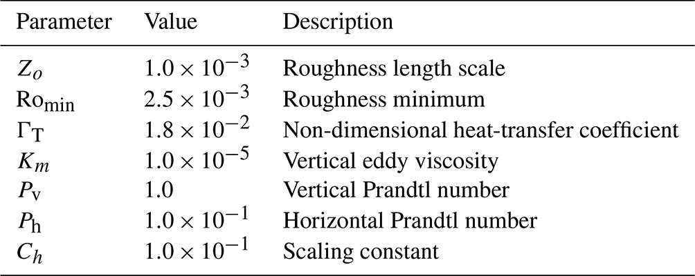
Table A1Turbulent transfer coefficient and mixing parameters used in this study.
The domain averaged temperature, potential density anomaly (referenced to 0 dbar), and flow speed are shown (Fig. B1) to document the stable model solution of the Thin Mobile run (as on 1 January 2016 00:00:00 UTC) from which the Mobile and Landfast runs are initialized. These diagnostics are also shown for the Mobile and Landfast runs for the entire duration (1 January 2016 00:00:00 UTC to 1 January 2017 00:00:00 UTC) of the simulation. We note that the progression of the modelling procedure (i.e. the Thin Mobile experiment, which is used to create the Mobile and Landfast experiments) described here is separate from the evolution the experiments aim to present (i.e. Landfast to Mobile to Thin Mobile).
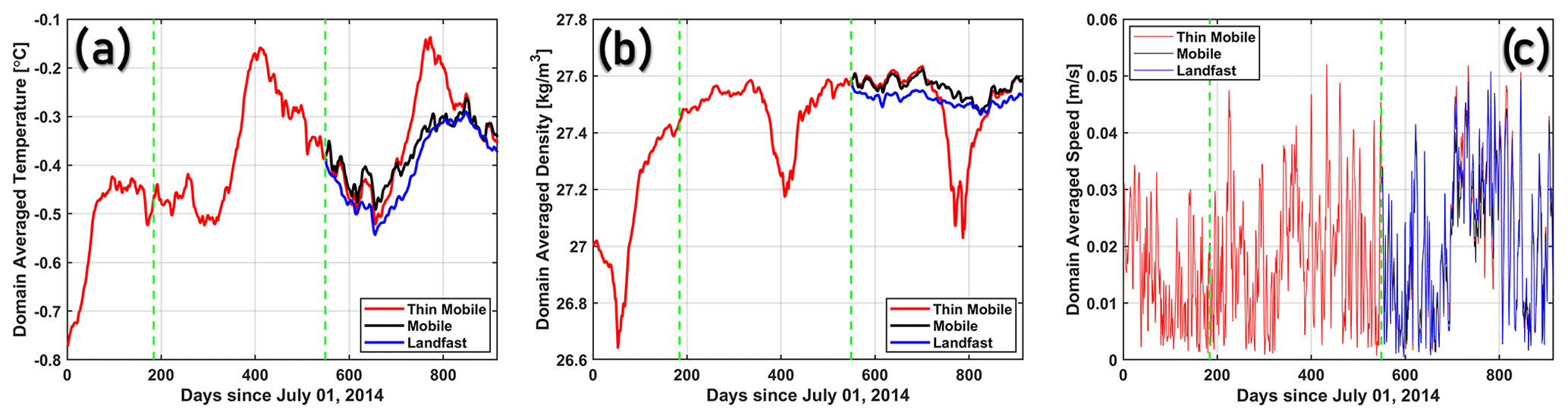
Figure B1Domain averaged temperature (a), potential density anomaly referenced to 0 dbar (b), and speed (c) for the Landfast, Mobile, and Thin Mobile runs. Green stippled lines represent days (since 1 July 2014) 184 and 549, which, respectively, denote the start of the 2015 and 2016 calendar year.
The primitive equations are solved in the spherical coordinate system, and the daily averaged seawater potential temperature (θ), salinity, east- and northward velocity (u and v, respectively), and the ice shelf basal melt rates used in this study are available as direct FVCOM model outputs. The u and v velocity components from the model output are transformed into Cartesian ux (x axis) and vy (y axis) components when presenting the diagnostics shown in Sect. 3. Moreover, the Ice Nudge module provides several prognostic variables related to ocean and sea ice–ocean (thermo)dynamics (see Prakash et al., 2022 for details). For instance, brine released during sea ice formation is captured using the variable virtual salt flux (FS), given in kilograms per square metre per second and converted to millimetres per day, and the variable salinity of the uppermost layer (Sw) is given in practical salinity units.
Calculating the overturning stream function (Ψ) and the overturning heat transport (Φ) normal to a cross-section in an unstructured grid representation of PF requires accounting for a non-uniform lateral and vertical cross-sectional geometry. First, the u, v, and θ fields are needed at each cell index along the transect (Fig. 1b) across which the calculations are made. (Note that the θ field stored on the FVCOM nodes are interpolated to the cell centres.) Then, the angle α between the x axis and the true eastward direction is computed and u and v are transformed into ux and vy as
where represents the transect cell index, the σ layer, and an index referencing the daily averaged model output intervals.
To integrate the transport normal to the transect, the flux is discretized laterally across the edge segments that are bounded by two successive cell indices, i and i+1. In the vertical, along the transect, the depth coordinates associated with the FVCOM nodes are interpolated to the cell centres. At each transect cell index, the difference between the successive sigma level depths at the cell centres gives the thickness of each of the 23 terrain-following σ layers. The angle ϕ between the x axis and the edge segment bounded by any two successive cell indices i, i+1, at all corresponding vertical levels j, with coordinates (xc(i,j), yc(i,j)) and (, ), respectively, is computed as
These angles are then used to compute the normal flow (u⟂) corresponding to each output interval τ and vertical level j at the two i, i+1 cell indices (abbreviated in the following by ⋄) as
The vertically integrated normal flow Ψz at each output interval τ is then computed as
where surf is the ocean surface or the base of the PGIS draft for sub-ice-shelf transects and H is the depth of the seafloor at cell indices i and i+1. represents the thickness of the corresponding σ layer j.
For each τ, the associated vertically integrated normal temperature flow Φz is calculated as
where ρ=1026 kg m−3 is the density of seawater, cp=3.97 kJ kg−1 ∘C−1 is its specific heat capacity, and ∘C is the freezing point of seawater at GL depth. Note that and for any cell index i and vertical level j represents the (heat) transport through the σ layer j at cell index i.
Then, for each τ, the vertically integrated mean flow , and the associated vertically integrated mean temperature flow normal to the discretized edge segment k bounded by cells i and i+1 is computed as
Thickness (dr(k), in metres) of the discretized flow sections bounded by cells i and i+1 is calculated as
Laterally integrating the vertically integrated mean normal (heat) transport () through the small edge segments k of thickness dr gives the overturning stream function Ψ (in cubic metres per second) and the associated overturning heat transport Φ (in kilojoules per second, converted to watts (W)), at each output interval τ, normal to the transect:
where, xw and xe, respectively, are the western and eastern PF boundaries at the transect.
Furthermore, evaluating Eqs. (C6), (C7), and (C8) only for the positive/negative values, or for both the positive and negative values of and , respectively, yields the mean inflow/outflow or the net flow in cubic metres per second, and the associated heat inflow (HIN)/outflow (HOUT) or the net heat flow (HNET) in kilojoules per second, converted to watts.
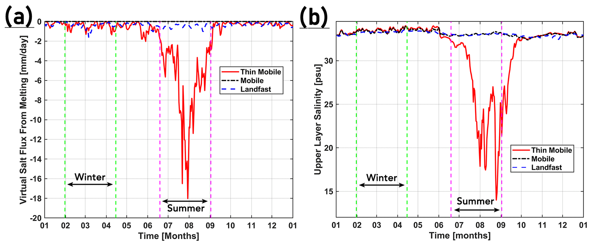
Figure D1Time series (2016) of the virtual salt flux due to sea ice melting (a) and the upper layer salinity (b) for the three experiments. (Note that a negative salt flux from sea ice melting indicates a positive freshwater flux.) The upper layer salinity is zoomed out from Fig. 9f to show the strong summer freshening in the Thin Mobile run. The stippled green and magenta lines in both panels indicate the span of the winter and summer seasons, respectively. Time series in both panels are shown for the same node on the Nares Strait section (Fig. 1b) near the Greenland coastline as in Fig. 9f.
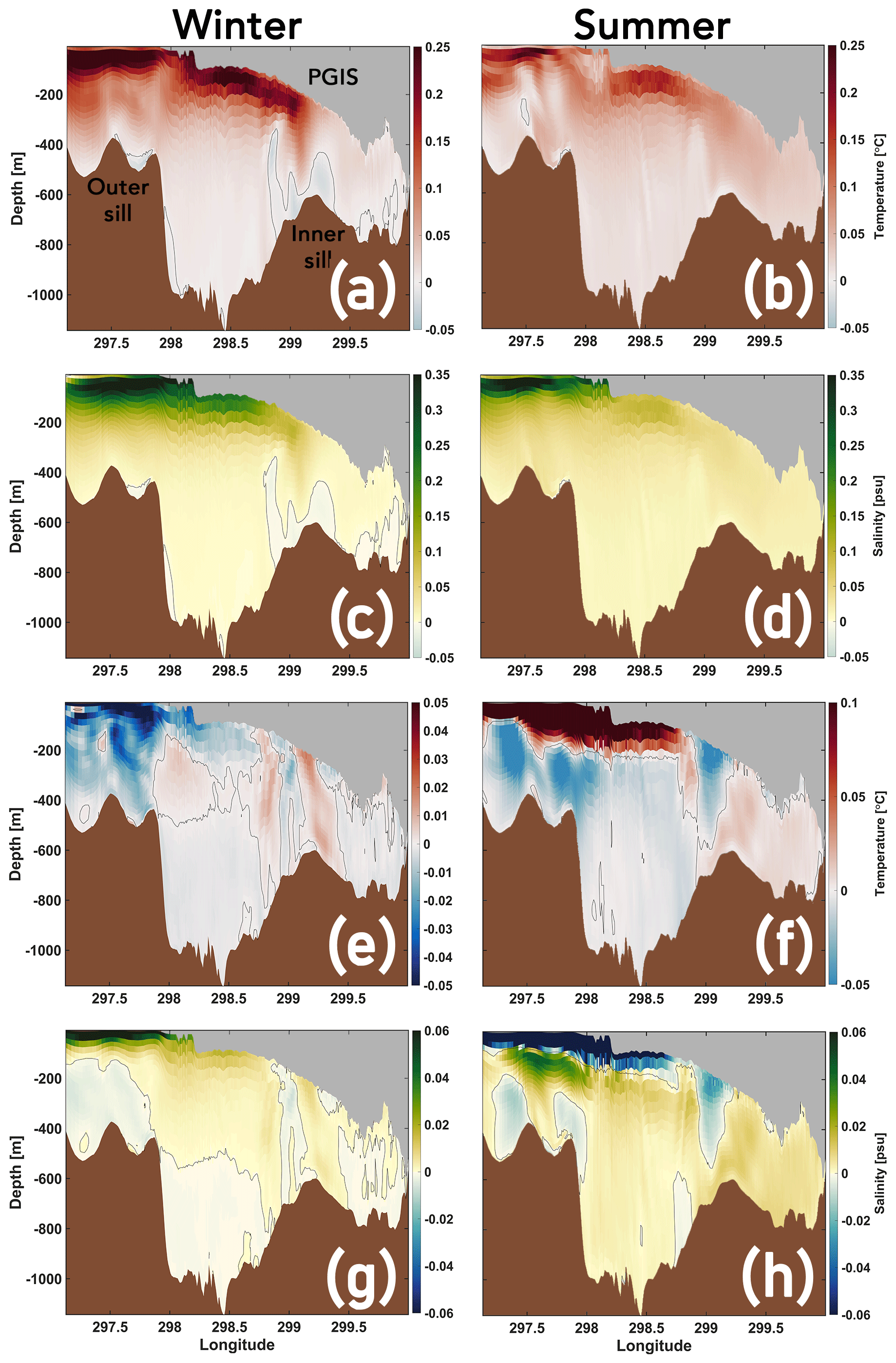
Figure D2Mobile – Landfast (a–d) and Thin Mobile – Mobile (e–h) seasonal mean temperature (a, b, e, f) and salinity (c, d, g, h) changes (see Fig. 10 for section location). The zero temperature and salinity difference contours are shown in black. When comparing (e) and (f), note the different range of scale used.
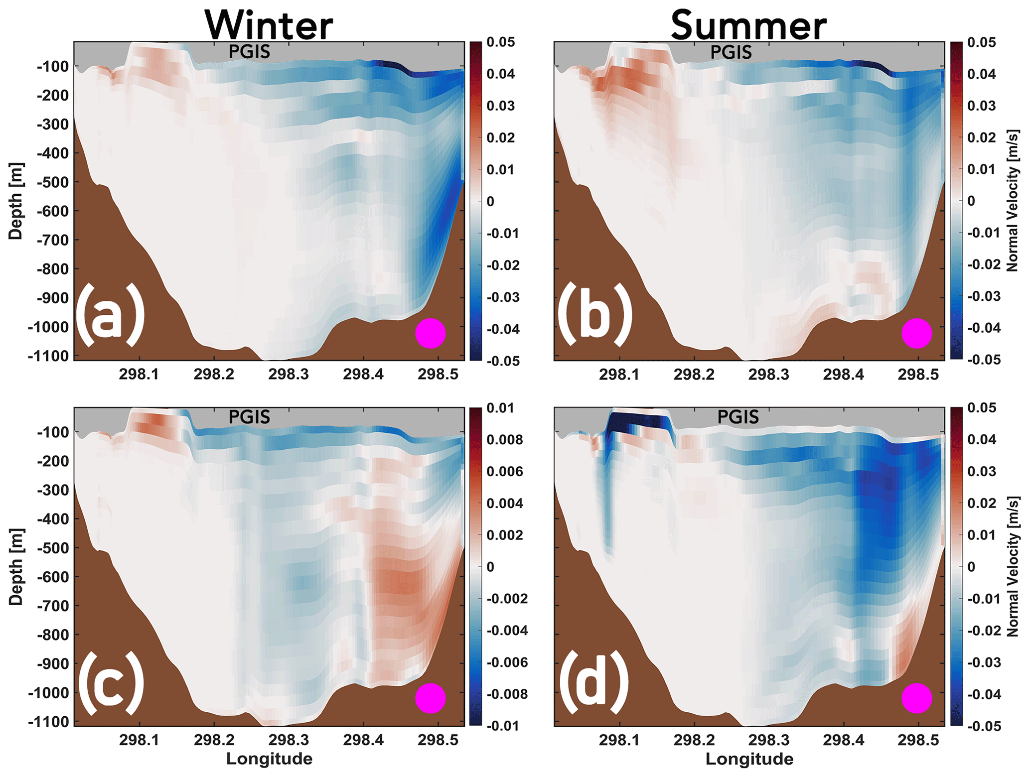
Figure D3Mobile – Landfast (a, b) and Thin Mobile – Mobile (c, d) seasonal mean outflow anomalies across the PGIS section (represented by magenta circles) shown in Fig. 1b. Negative values correspond to strengthening of flow out of the PGIS cavity, whereas positive values correspond to its weakening (and not an inflow), as detailed in Appendix C. Note the different scale used in (c).
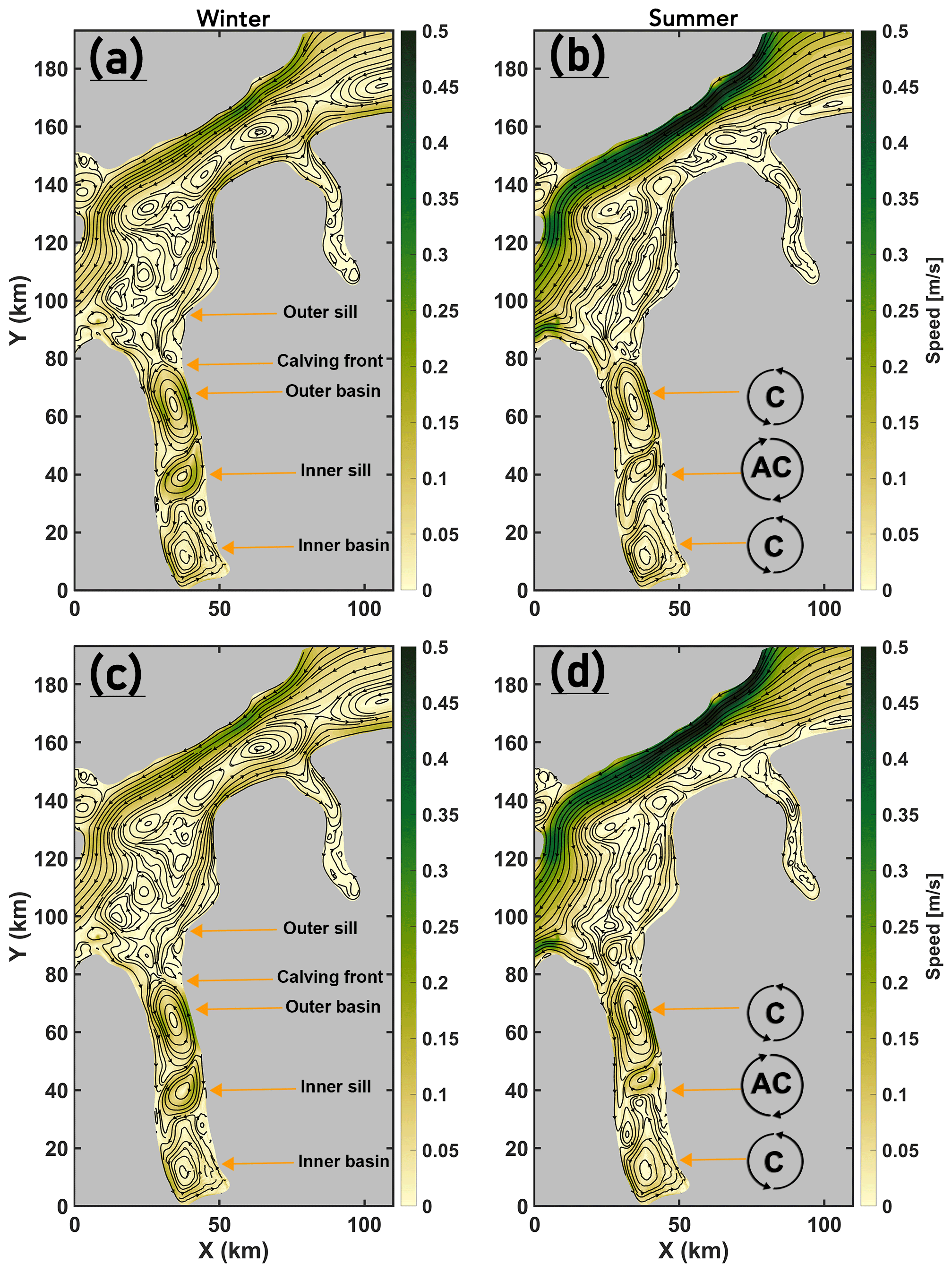
Figure D4Depth averaged seasonal mean speed of the modelled ocean velocities for the Mobile (a, b) and Thin Mobile (c, d) experiments with mean streamlines overlaid (see Fig. 3 for location). Selected topographic features in PF are labelled in (a) and (c). Location of the cyclonic (C) and anticyclonic (AC) gyres in PF are shown in (b) and (d). Note that the streamlines were generated using the “streamslice” function on Matlab and, as such, are not well-defined conservative stream functions but are used to assist in visualizing the circulation patterns.
Table E1Annual, winter, and summer mean PGIS basal melt rates (, in metres per year) for the Landfast, Mobile, and Thin Mobile experiments. averaged over the entire ice shelf is denoted by the subscript “pgis”, whereas the subscript “200” denotes that is averaged over (only) the >200 m region of the ice shelf.
The open source code Finite Volume Community Ocean Model version 4.0 (FVCOM4.0) that has been augmented to allow the inclusion of ice shelf cavities is available from Zhou and Hattermann (2020). The Ice Nudge module is as described in Prakash et al. (2022). All model input files that are required to run the experiments will be made freely available upon request.
AP conceptualized the study and, together with QZ and TH, designed the framework for the Ice Nudge experiments. AP ran the simulations and interpreted the model output with advice from QZ and TH. AP carried out the model analysis with supervision from TH. AP and NK wrote the manuscript with contributions from QZ and TH.
The contact author has declared that none of the authors has any competing interests.
Publisher’s note: Copernicus Publications remains neutral with regard to jurisdictional claims made in the text, published maps, institutional affiliations, or any other geographical representation in this paper. While Copernicus Publications makes every effort to include appropriate place names, the final responsibility lies with the authors.
This work was associated with the Research Council of Norway (RCN) project no. 280727 (PI: Rune Grand Graversen). Qin Zhou is supported by the RCN project nos. 244319 and 295075. Tore Hattermann is supported by the RCN project no. 314570. The simulations were performed on resources provided by UNINETT Sigma2 – the National Infrastructure for High Performance Computing and Data Storage in Norway. The supercomputers Fram, Betzy, and the NIRD storage facilities were used under the projects nos. NN9348K, NN9824K, and NS9063K, respectively. We thank the two anonymous reviewers for their insightful comments and suggestions, which helped us in improving the manuscript.
This research has been supported by the Svenska Forskningsrådet Formas (grant no. 2017-00665).
The article processing charges for this open-access publication were covered by Stockholm University.
This paper was edited by Yevgeny Aksenov and reviewed by two anonymous referees.
Aschwanden, A., Fahnestock, M. A., Truffer, M., Brinkerhoff, D. J., Hock, R., Khroulev, C., Mottram, R., and Khan, S. A.: Contribution of the Greenland Ice Sheet to sea level over the next millennium, Sci. Adv., 5, eaav9396, https://doi.org/10.1126/sciadv.aav9396, 2019. a
Cai, C., Rignot, E., Menemenlis, D., and Nakayama, Y.: Observations and modeling of ocean-induced melt beneath Petermann Glacier Ice Shelf in northwestern Greenland, Geophys. Res. Lett., 44, 8396–8403, 2017. a, b
Carroll, D., Sutherland, D. A., Shroyer, E. L., Nash, J. D., Catania, G. A., and Stearns, L. A.: Modeling turbulent subglacial meltwater plumes: Implications for fjord-scale buoyancy-driven circulation, J. Phys. Oceanogr., 45, 2169–2185, 2015. a
Carroll, D., Sutherland, D. A., Shroyer, E. L., Nash, J. D., Catania, G. A., and Stearns, L. A.: Subglacial discharge-driven renewal of tidewater glacier fjords, J. Geophys. Res.-Oceans, 122, 6611–6629, 2017. a
Chen, C., Huang, H., Beardsley, R. C., Liu, H., Xu, Q., and Cowles, G.: A finite volume numerical approach for coastal ocean circulation studies: Comparisons with finite difference models, J. Geophys. Res.-Oceans, 112, C03018, https://doi.org/10.1029/2006JC003485, 2007. a, b, c
Chen, X., Zhang, X., Church, J. A., Watson, C. S., King, M. A., Monselesan, D., Legresy, B., and Harig, C.: The increasing rate of global mean sea-level rise during 1993–2014, Nat. Clim. Change, 7, 492–495, 2017. a
Falkner, K. K., Melling, H., Münchow, A. M., Box, J. E., Wohlleben, T., Johnson, H. L., Gudmandsen, P., Samelson, R., Copland, L., Steffen, K., Rignot, E., and Higgins, A. K.: Context for the recent massive Petermann Glacier calving event, Eos, Transactions American Geophysical Union, 92, 117–118, 2011. a
Fraser, N. J., Inall, M. E., Magaldi, M. G., Haine, T. W., and Jones, S. C.: Wintertime fjord-shelf interaction and ice sheet melting in southeast Greenland, J. Geophys. Res.-Oceans, 123, 9156–9177, 2018. a
Galperin, B., Kantha, L., Hassid, S., and Rosati, A.: A quasi-equilibrium turbulent energy model for geophysical flows, J. Atmos. Sci., 45, 55–62, https://doi.org/10.1175/1520-0469(1988)045<0055:AQETEM>2.0.CO;2, 1988. a
Gwyther, D. E., Galton-Fenzi, B. K., Dinniman, M. S., Roberts, J. L., and Hunter, J. R.: The effect of basal friction on melting and freezing in ice shelf–ocean models, Ocean Model., 95, 38–52, 2015. a
Hager, A. O., Sutherland, D. A., Amundson, J. M., Jackson, R. H., Kienholz, C., Motyka, R. J., and Nash, J. D.: Subglacial discharge reflux and buoyancy forcing drive seasonality in a silled glacial fjord, J. Geophys. Res.-Oceans, 127, e2021JC018355, https://doi.org/10.1029/2021JC018355, 2022. a, b
Hattermann, T., Isachsen, P. E., von Appen, W.-J., Albretsen, J., and Sundfjord, A.: Eddy-driven recirculation of Atlantic water in Fram Strait, Geophys. Res. Lett., 43, 3406–3414, 2016. a
Heuzé, C., Wåhlin, A., Johnson, H. L., and Münchow, A.: Pathways of meltwater export from Petermann Glacier, Greenland, J. Phys. Oceanogr., 47, 405–418, 2017. a, b, c, d
Hill, E. A., Carr, J. R., and Stokes, C. R.: A review of recent changes in major marine-terminating outlet glaciers in Northern Greenland, Front. Earth Sci., 4, 111, https://doi.org/10.3389/feart.2016.00111, 2017. a
Hill, E. A., Carr, J. R., Stokes, C. R., and Gudmundsson, G. H.: Dynamic changes in outlet glaciers in northern Greenland from 1948 to 2015, The Cryosphere, 12, 3243–3263, https://doi.org/10.5194/tc-12-3243-2018, 2018. a, b
Holland, D. M. and Jenkins, A.: Modeling thermodynamic ice–ocean interactions at the base of an ice shelf, J. Phys. Oceanogr., 29, 1787–1800, 1999. a, b
Holland, M. M., Clemens-Sewall, D., Landrum, L., Light, B., Perovich, D., Polashenski, C., Smith, M., and Webster, M.: The influence of snow on sea ice as assessed from simulations of CESM2, The Cryosphere, 15, 4981–4998, https://doi.org/10.5194/tc-15-4981-2021, 2021. a
Hunke, E. C., Lipscomb, W. H., Turner, A. K., Jeffery, N., and Elliott, S.: Cice: the los alamos sea ice model documentation and software user’s manual version 4.1 la-cc-06-012, T-3 Fluid Dynamics Group, Los Alamos National Laboratory, 675, 500, 2010. a, b
Jackson, R. H., Straneo, F., and Sutherland, D. A.: Externally forced fluctuations in ocean temperature at Greenland glaciers in non-summer months, Nat. Geosci., 7, 503–508, 2014. a
Jakobsson, M., Mayer, L. A., Bringensparr, C., Castro, C. F., Mohammad, R., Johnson, P., Ketter, T., Accettella, D., Amblas, D., An, L., Arndt, J. E., Canals, M., Casamor, J. L., Chauché, N., Coakley, B., Danielson, S., Demarte, M., Dickson, M.-L., Dorschel, B., Dowdeswell, J. A., Dreutter, S., Fremand, A. C., Gallant, D., Hall, J. K., Hehemann, L., Hodnesdal, H., Hong, J., Ivaldi, R., Kane, E., Klaucke, I., Krawczyk, D. W., Kristoffersen, Y., Kuipers, B. R., Millan, R., Masetti, G., Morlighem, M., Noormets, R., Prescott, M. M., Rebesco, M., Rignot, E., Semiletov, I., Tate, A. J., Travaglini, P., Velicogna, I., Weatherall, P., Weinrebe, W., Willis, J. K., Wood, M., Zarayskaya, Y., Zhang, T., Zimmermann, M., and Zinglersen, K. B.: The international bathymetric chart of the Arctic Ocean version 4.0, Sci. Data, 7, 1–14, 2020a. a
Jakobsson, M., Mayer, L. A., Nilsson, J., Stranne, C., Calder, B., O’Regan, M., Farrell, J. W., Cronin, T. M., Brüchert, V., Chawarski, J., Eriksson, B., Fredriksson, J., Gemery, L., Glueder, A., Holmes, F. A., Jerram, K., Kirchner, N., Mix, A., Muchowski, J., Prakash, A., Reilly, B., Thornton, B., Ulfsbo, A., Weidner, E., Åkesson, H., Handl, T., Ståhl, E., Boze, L.-G., Reed, S., West, G., and Padman, J.: Ryder Glacier in northwest Greenland is shielded from warm Atlantic water by a bathymetric sill, Commun. Earth Environ., 1, 1–10, 2020b. a
Jenkins, A., Hellmer, H. H., and Holland, D. M.: The role of meltwater advection in the formulation of conservative boundary conditions at an ice–ocean interface, J. Phys. Oceanogr., 31, 285–296, 2001. a, b
Johnson, H., Münchow, A., Falkner, K., and Melling, H.: Ocean circulation and properties in Petermann Fjord, Greenland, J. Geophys. Res.-Oceans, 116, C01003, https://doi.org/10.1029/2010JC006519, 2011. a, b, c, d, e, f
Kacimi, S. and Kwok, R.: Arctic Snow Depth, Ice Thickness, and Volume From ICESat-2 and CryoSat-2: 2018–2021, Geophys. Res. Lett., 49, e2021GL097448, https://doi.org/10.1029/2021GL097448, 2022. a, b
Kajanto, K., Straneo, F., and Nisancioglu, K.: Impact of icebergs on the seasonal submarine melt of Sermeq Kujalleq, The Cryosphere, 17, 371–390, https://doi.org/10.5194/tc-17-371-2023, 2023. a
Keen, A., Blockley, E., Bailey, D. A., Boldingh Debernard, J., Bushuk, M., Delhaye, S., Docquier, D., Feltham, D., Massonnet, F., O'Farrell, S., Ponsoni, L., Rodriguez, J. M., Schroeder, D., Swart, N., Toyoda, T., Tsujino, H., Vancoppenolle, M., and Wyser, K.: An inter-comparison of the mass budget of the Arctic sea ice in CMIP6 models, The Cryosphere, 15, 951–982, https://doi.org/10.5194/tc-15-951-2021, 2021. a
Kwok, R.: Variability of Nares Strait ice flux, Geophys. Res. Lett., 32, L24502, https://doi.org/10.1029/2005GL024768, 2005. a, b
Kwok, R.: Arctic sea ice thickness, volume, and multiyear ice coverage: losses and coupled variability (1958–2018), Environ. Res. Lett., 13, 105005, https://doi.org/10.1088/1748-9326/aae3ec, 2018. a
Kwok, R., Toudal Pedersen, L., Gudmandsen, P., and Pang, S.: Large sea ice outflow into the Nares Strait in 2007, Geophys. Res. Lett., 37, https://doi.org/10.1029/2009GL041872, 2010. a, b, c, d
Maslanik, J., Stroeve, J., Fowler, C., and Emery, W.: Distribution and trends in Arctic sea ice age through spring 2011, Geophys. Res. Lett., 38, L13502, https://doi.org/10.1029/2011GL047735, 2011. a
Mellor, G. L. and Yamada, T.: Development of a turbulence closure model for geophysical fluid problems, Rev. Geophys., 20, 851–875, 1982. a
Meredith, M., Sommerkorn, M., Cassotta, S., Derksen, C., Ekaykin, A., Hollowed, A., Kofinas, G., Mackintosh, A., Melbourne-Thomas, J., Muelbert, M. M. C., Ottersen, G., Pritchard, H., and Schuur, E. A. G.: Polar Regions, in: IPCC Special Report on the Ocean and Cryosphere in a Changing Climate, edited by: Pörtner, H.-O., Roberts, D. C., Masson-Delmotte, V., Zhai, P., Tignor, M., Poloczanska, E., Mintenbeck, K., Alegría, A., Nicolai, M., Okem, A., Petzold, J., Rama, B., and Weyer, N. M., 203–320, Cambridge University Press, Cambridge, United Kingdom and New York, NY, USA, https://doi.org/10.1017/9781009157964.005, 2019. a
Moore, G. and McNeil, K.: The early collapse of the 2017 Lincoln Sea ice arch in response to anomalous sea ice and wind forcing, Geophys. Res. Lett., 45, 8343–8351, 2018. a, b
Moore, G., Howell, S., Brady, M., Xu, X., and McNeil, K.: Anomalous collapses of Nares Strait ice arches leads to enhanced export of Arctic sea ice, Nat. Commun., 12, 1–8, 2021. a, b, c, d, e, f, g, h
Morlighem, M., Williams, C. N., Rignot, E., An, L., Arndt, J. E., Bamber, J. L., Catania, G., Chauché, N., Dowdeswell, J. A., Dorschel, B., Fenty, I., Hogan, K., Howat, I., Hubbard, A., Jakobsson, M., Jordan, T. M., Kjeldsen, K. K., Millan, R., Mayer, L., Mouginot, J., Noël, B. P. Y., Cofaigh, C. Ó., Palmer, S., Rysgaard, S., Seroussi, H., Siegert, M. J., Slabon, P., Straneo, F., van den Broeke, M. R., Weinrebe, W., Wood, M., and Zinglersen, K. B.: BedMachine v3: Complete bed topography and ocean bathymetry mapping of Greenland from multibeam echo sounding combined with mass conservation, Geophys. Res. Lett., 44, 11051–11061, https://doi.org/10.1002/2017GL074954, 2017. a
Mouginot, J., Rignot, E., Bjørk, A. A., Van den Broeke, M., Millan, R., Morlighem, M., Noël, B., Scheuchl, B., and Wood, M.: Forty-six years of Greenland Ice Sheet mass balance from 1972 to 2018, P. Natl. Acad. Sci. USA, 116, 9239–9244, 2019. a, b, c
Münchow, A.: Volume and freshwater flux observations from Nares Strait to the west of Greenland at daily time scales from 2003 to 2009, J. Phys. Oceanogr., 46, 141–157, 2016. a
Münchow, A., Padman, L., and Fricker, H. A.: Interannual changes of the floating ice shelf of Petermann Gletscher, North Greenland, from 2000 to 2012, J. Glaciol., 60, 489–499, 2014. a
Noël, B., van de Berg, W. J., Lhermitte, S., and van den Broeke, M. R.: Rapid ablation zone expansion amplifies north Greenland mass loss, Sci. Adv., 5, eaaw0123, https://doi.org/10.1126/sciadv.aaw0123, 2019. a
Notz, D. and SIMIP Community: Arctic sea ice in CMIP6, Geophys. Res. Lett., 47, e2019GL086749, https://doi.org/10.1029/2019GL086749, 2020. a, b
Padman, L. and Erofeeva, S.: A barotropic inverse tidal model for the Arctic Ocean, Geophys. Res. Lett., 31, L02303, https://doi.org/10.1029/2003GL019003, 2004. a
Peralta-Ferriz, C. and Woodgate, R. A.: Seasonal and interannual variability of pan-Arctic surface mixed layer properties from 1979 to 2012 from hydrographic data, and the dominance of stratification for multiyear mixed layer depth shoaling, Prog. Oceanogr., 134, 19–53, 2015. a
Pörtner, H.-O., Roberts, D. C., Masson-Delmotte, V., Zhai, P., Tignor, M., Poloczanska, E., and Weyer, N.: The ocean and cryosphere in a changing climate, IPCC Special Report on the Ocean and Cryosphere in a Changing Climate, https://www.ipcc.ch/site/assets/uploads/sites/3/2022/03/00_SROCC_Frontmatter_FINAL.pdf (last access: 8 December 2023), 2019. a
Prakash, A., Zhou, Q., Hattermann, T., Bao, W., Graversen, R., and Kirchner, N.: A nested high-resolution unstructured grid 3-D ocean-sea ice-ice shelf setup for numerical investigations of the Petermann ice shelf and fjord, MethodsX, 9, 101668, https://doi.org/10.1016/j.mex.2022.101668, 2022. a, b, c, d, e, f, g, h, i, j, k, l, m, n, o, p, q
Rignot, E. and Steffen, K.: Channelized bottom melting and stability of floating ice shelves, Geophys. Res. Lett., 35, L02503, https://doi.org/10.1029/2007GL031765, 2008. a, b
Rückamp, M., Neckel, N., Berger, S., Humbert, A., and Helm, V.: Calving induced speedup of Petermann glacier, J. Geophys. Res.-Earth, 124, 216–228, 2019. a
Ryan, P. A. and Münchow, A.: Sea ice draft observations in N ares S trait from 2003 to 2012, J. Geophys. Res.-Oceans, 122, 3057–3080, 2017. a, b
Sasgen, I., Wouters, B., Gardner, A. S., King, M. D., Tedesco, M., Landerer, F. W., Dahle, C., Save, H., and Fettweis, X.: Return to rapid ice loss in Greenland and record loss in 2019 detected by the GRACE-FO satellites, Commun. Earth Environ., 1, 1–8, 2020. a
Shroyer, E. L., Padman, L., Samelson, R., Münchow, A., and Stearns, L. A.: Seasonal control of Petermann Gletscher ice-shelf melt by the ocean's response to sea-ice cover in Nares Strait, J. Glaciol., 63, 324–330, 2017. a, b, c, d, e, f, g, h
Shu, Q., Wang, Q., Årthun, M., Wang, S., Song, Z., Zhang, M., and Qiao, F.: Arctic Ocean Amplification in a warming climate in CMIP6 models, Sci. Adv., 8, eabn9755, https://doi.org/10.1126/sciadv.abn9755, 2022. a, b
Slater, D. A., Straneo, F., Felikson, D., Little, C. M., Goelzer, H., Fettweis, X., and Holte, J.: Estimating Greenland tidewater glacier retreat driven by submarine melting, The Cryosphere, 13, 2489–2509, https://doi.org/10.5194/tc-13-2489-2019, 2019. a
Smagorinsky, J.: General circulation experiments with the primitive equations: I. The basic experiment, Mon. Weather Rev., 91, 99–164, 1963. a
Straneo, F. and Cenedese, C.: The dynamics of Greenland's glacial fjords and their role in climate, Annu. Rev. Mar. Sci., 7, 89–112, 2015. a
The IMBIE Team: Mass balance of the Greenland Ice Sheet from 1992 to 2018, Nature, 579, 233–239, https://doi.org/10.1038/s41586-019-1855-2, 2020. a
Tinto, K. J., Bell, R. E., Cochran, J. R., and Münchow, A.: Bathymetry in Petermann fjord from Operation IceBridge aerogravity, Earth Planet. Sc. Lett., 422, 58–66, 2015. a, b
Tsamados, M., Feltham, D., Petty, A., Schroeder, D., and Flocco, D.: Processes controlling surface, bottom and lateral melt of Arctic sea ice in a state of the art sea ice model, Philos. T. Roy. Soc. A, 373, 20140167, https://doi.org/10.1098/rsta.2014.0167, 2015. a
Wang, M. and Overland, J. E.: A sea ice free summer Arctic within 30 years: An update from CMIP5 models, Geophys. Res. Lett., 39, L07502, https://doi.org/10.1029/2009GL037820, 2012. a
Washam, P., Münchow, A., and Nicholls, K. W.: A decade of ocean changes impacting the ice shelf of Petermann Gletscher, Greenland, J. Phys. Oceanogr., 48, 2477–2493, 2018. a, b, c
Washam, P., Nicholls, K. W., Münchow, A., and Padman, L.: Tidal modulation of buoyant flow and basal melt beneath Petermann Gletscher Ice Shelf, Greenland, J. Geophys. Res.-Oceans, 125, e2020JC016427, https://doi.org/10.1029/2020JC016427, 2020. a, b
Wilson, N., Straneo, F., and Heimbach, P.: Satellite-derived submarine melt rates and mass balance (2011–2015) for Greenland's largest remaining ice tongues, The Cryosphere, 11, 2773–2782, https://doi.org/10.5194/tc-11-2773-2017, 2017. a, b, c
Wood, M., Rignot, E., Fenty, I., An, L., Bjørk, A., van den Broeke, M., Cai, C., Kane, E., Menemenlis, D., Millan, R., Morlighem, M., Mouginot, J., Noël, B., Scheuchl, B., Velicogna, I., Willis, J. K., and Zhang, H.: Ocean forcing drives glacier retreat in Greenland, Sci. Adv., 7, eaba7282, https://doi.org/10.1126/sciadv.aba7282, 2021. a
Zhou, Q. and Hattermann, T.: Modeling ice shelf cavities in the unstructured-grid, Finite Volume Community Ocean Model: Implementation and effects of resolving small-scale topography, Ocean Model., 146, 101536, https://doi.org/10.1016/j.ocemod.2019.101536, 2020. a, b, c, d, e
- Abstract
- Introduction
- Methods
- Results
- Discussion
- Summary and concluding remarks
- Appendix A: Model setup
- Appendix B: Model stability
- Appendix C: Model output and diagnostics
- Appendix D: Supplementary figures
- Appendix E: Melt rate (summary) table
- Code and data availability
- Author contributions
- Competing interests
- Disclaimer
- Acknowledgements
- Financial support
- Review statement
- References