the Creative Commons Attribution 4.0 License.
the Creative Commons Attribution 4.0 License.
 | 08 Dec 2023
Multidecadal variability and predictability of Antarctic sea ice in the GFDL SPEAR_LO model
Liping Zhang
Thomas L. Delworth
Xiaosong Yang
Fanrong Zeng
Masami Nonaka
Swadhin K. Behera
Using a state-of-the-art coupled general circulation model, physical processes underlying Antarctic sea ice multidecadal variability and predictability are investigated. Our model simulations constrained by atmospheric reanalysis and observed sea surface temperature broadly capture a multidecadal variability in the observed sea ice extent (SIE) with a low sea ice state (late 1970s–1990s) and a high sea ice state (2000s–early 2010s), although the model overestimates the SIE decrease in the Weddell Sea around the 1980s. The low sea ice state is largely due to the deepening of the mixed layer and the associated deep convection that brings subsurface warm water to the surface. During the high sea ice period (post-2000s), the deep convection substantially weakens, so surface wind variability plays a greater role in the SIE variability. Decadal retrospective forecasts started from the above model simulations demonstrate that the Antarctic sea ice multidecadal variability can be skillfully predicted 6–10 years in advance, showing a moderate correlation with the observation. Ensemble members with a deeper mixed layer and stronger deep convection tend to predict a larger sea ice decrease in the 1980s, whereas members with a larger surface wind variability tend to predict a larger sea ice increase after the 2000s. Therefore, skillful simulation and prediction of the Antarctic sea ice multidecadal variability require accurate simulation and prediction of the mixed layer, deep convection, and surface wind variability in the model.
- Article
(7593 KB) - Full-text XML
-
Supplement
(2225 KB) - BibTeX
- EndNote


Antarctic sea ice plays key roles in exchanging heat, momentum, freshwater, and gases between the atmosphere and the ocean in the Southern Ocean. The formation of sea ice near the Antarctic coast generates high-salinity dense water or high-salinity shelf water that flows into the bottom of the Southern Ocean (e.g., Antarctic Bottom Water; Orsi et al., 1999) and affects global thermohaline circulation. Antarctic sea ice extent (SIE) undergoes substantial seasonal-to-interannual variations (e.g., Yuan and Martinson, 2000; Cavalieri et al., 2003) and shows a slightly increasing trend until 2015 (e.g., Yuan et al., 2017; Parkinson, 2019). This contrasts with a significant SIE decrease in the early and middle 20th century, estimated from century-long reconstructed SIE data (Fogt et al., 2022). This implies that low-frequency variability beyond a decadal timescale may exist in the Antarctic SIE. Satellite observations show that the Antarctic SIE reaches a record high in 2014 but abruptly declines and reaches a record low in early 2022 (Simpkins, 2023). The Weddell Sea contributes the most to the total sea ice decrease (Turner et al., 2020). The recent Antarctic SIE decrease is attributed to several physical processes, including the upper Southern Ocean warming (Meehl et al., 2019; Zhang et al., 2022b), anomalous warm air advection from the north (Turner et al., 2017) associated with atmospheric teleconnection from the tropics (Wang et al., 2019), and weakening of the midlatitude westerlies (Stuecker et al., 2017; Schlosser et al., 2018) linked to a negative phase of the Southern Annual Mode (SAM; Thompson and Wallace, 2000) induced by the weakening of the polar stratospheric vortex (Wang et al., 2019). It is still unclear whether the recent SIE decrease is a part of interannual or lower-frequency variability or climate change (Eayrs et al., 2021).
Most coupled general circulation models (CGCMs) simulate a decreasing trend of the Antarctic SIE in response to both increasing greenhouse gases and stratospheric ozone depletion. The positive SIE trend observed in the past 3 decades until 2015 cannot be solely explained by anthropogenic forcings but may be attributed to natural variability (Polvani and Smith, 2013). For example, Goosse and Zunz (2014) discussed the role of positive ice–ocean feedback in the amplification of sea ice increase using a CGCM simulation. Once the sea ice starts to increase, the brine released from the sea ice can be transported downward to deeper layers and not incorporated back into the mixed layer. This leads to a decrease in the surface salinity, an increase in the surface stratification, and thus the reduced vertical ocean heat transport, resulting in a further increase in the sea ice.
Open-ocean deep convection (Gordon, 1978; Killworth, 1983; Akitomo et al., 1995) in the Southern Ocean is also important for Antarctic sea ice variability. For example, Goosse and Fichefet (2001) examined the role of the deep convection in the formation of Weddell Polynya (i.e., open water area enclosed by sea ice) using an ocean–ice model. They found that the surface salinity increase owing to the brine release during the sea ice formation tends to induce the deep convection and entrain the relatively warm water from the subsurface ocean to the surface mixed layer, responsible for the sea ice decrease. The modifications of the mixed layer are much larger than the aforementioned positive feedback process by Goosse and Zunz (2014), which mainly occurs near the sea ice edge over a wide domain. The link between the Weddell Polynya and the open-ocean deep convection is widely discussed in observational and modeling studies (e.g., Gordon et al., 2007; Cheon et al., 2014, 2015). Recently, Zhang et al. (2019) pointed out that the observed SST cooling and trends of increasing sea ice in the Ross and Weddell seas can be reproduced in the CGCM where they start the simulations from an active phase of the deep convection.
On the other hand, surface wind variability also contributes to Antarctic sea ice variability. Turner et al. (2016) attributed the positive SIE trend in the Ross Sea to stronger southerly winds associated with a deepening of the Amundsen Sea Low, which are linked to a negative phase of the Interdecadal Pacific Oscillation (IPO; Power et al., 1999; Meehl et al., 2016) and a positive phase of the Atlantic Multidecadal Oscillation (AMO; Li et al., 2014). The stronger southerly winds tend to enhance northward sea ice advection and increase sea ice concentration in the Ross Sea (Holland and Kwok, 2012). Using a CGCM constrained by atmospheric reanalysis surface winds and observed SST, Blanchard-Wrigglesworth et al. (2021) confirmed the influences of surface winds and SST in the Southern Ocean on the Antarctic SIE trend and variability. However, their simulations could not well reproduce the low sea ice state in the 1980s and the increasing SIE trend afterwards. Sun and Eisenman (2021) modified the simulations by replacing the model sea ice velocity with the observed sea ice motion and found that their new simulations can capture the Antarctic trend of increasing sea ice from 1992 to 2015. The failure of the model in simulating the trend of increasing sea ice may be due to the model biases in the sea ice drift velocity.
Several studies have reported skillful predictions of regional and pan-Antarctic SIE variability at seasonal-to-interannual timescales (Guemas et al., 2014, 2016; Marchi et al., 2019; Morioka et al., 2019, 2021; Bushuk et al., 2021), and prediction skills of summertime sea ice are generally lower than those of wintertime sea ice. However, few studies have examined the multi-year to decadal predictability of the Antarctic SIE. Yang et al. (2016) provided a broad assessment of the Antarctic SIE predictability using decadal hindcasts from 11 Coupled Model Intercomparison Project Phase 5 (CMIP5) models. They concluded that most of the CMIP5 models do not show promising prediction skills for the Antarctic SIE anomalies. The prediction skills are much lower than the persistence prediction using the observed SIE anomalies. Most of the CMIP5 models cannot predict the trend of increasing Antarctic SIE in the past 3 decades. When a linear trend is removed from the SIE anomalies, the prediction skills become higher in the Ross Sea and the Weddell Sea. The prediction skills in the initialized hindcasts tend to be higher than those in the uninitialized hindcasts. These results are consistent with a former study (Zunz et al., 2015) that showed a skillful prediction of the multi-year Antarctic SIE variability by initializing the model surface air temperature. Recently, Morioka et al. (2022) demonstrated that ocean and sea ice initializations in their CGCM improve decadal sea ice prediction skills in the west Antarctic seas. They discussed the improvement of prediction skills for the regional sea ice, in particular after 2005 when the subsurface ocean observations increased. However, the model could not capture the sea ice decrease in the 1980s owing to lack of subsurface ocean observations used for their data assimilation, so we need further efforts to improve our understanding of multidecadal sea ice variability and predictability.
In this study, we attempt to address the following two scientific questions: what are relative importance of the Southern Ocean deep convection and the atmospheric variability in the Antarctic SIE multidecadal variability, and how far and skillfully can the Antarctic sea ice multidecadal variability be predicted and what are the underlying physical processes? To this end, we examine the Antarctic sea ice multidecadal variability and predictability using the GFDL's (Geophysical Fluid Dynamics Laboratory) newly developed Seamless System for Prediction and Earth System Research (SPEAR; Delworth et al., 2020) model. We compare the observation data and model simulations constrained by atmospheric reanalysis surface winds and temperature and observed SST to evaluate how reasonably the model simulates the observed SIE variability. We also clarify the relative importance of atmosphere and ocean in the Antarctic SIE multidecadal variability. Using the decadal retrospective forecasts started from the above constrained model simulations, we attempt to understand to what extent the multidecadal sea ice variability can skillfully be predicted. This paper is organized as follows: Sect. 2 describes the observational data and model experiments performed in this study. In Sect. 3, we provide all the observational and model results. In Sect. 4, we put them into historical context and discuss the remaining issues to be addressed in future work.
2.1 Observation data
We obtained monthly sea ice concentration (SIC) from the Hadley Centre Global Sea Ice and Sea Surface Temperature version 1 (HadISST1; Rayner et al., 2003) and version 2 (HadISST2; Titchner and Rayner, 2014), which have a horizontal resolution of 1∘. We analyzed the SIC data during 1958–2020 for HadISST1 and 1958–2019 for HadISST2 to compare them with the SPEAR simulations described below. Since HadISST1 covers a slightly longer period than HadISST2, we used the SIC data from HadISST1 to perform a persistence decadal retrospective forecast in which the observed SIC anomaly for each year of 1961–2011 is assumed to persist over the next 10 years.
It should be noted that HadISST2 provides a more consistent sea ice record than HadISST1 because HadISST2 employs new data sources, new bias adjustments, and new methods to estimate the sea ice concentration based on the sea ice edge information. These updates lead to a higher sea ice concentration and a larger extent for some regions and periods in HadISST2 than HadISST1 (Titchner and Rayner, 2014). Also, both HadISST1 and HadISST2 derive the SIC data indirectly using the monthly climatology of the observations for each decade before the advent of satellite imagery in 1973. Therefore, the SIC data do not include any interannual variability before the early 1970s but give a general indication of sea ice variations on decadal timescales. Due to these bias adjustments, HadISST2 tends to show larger SIE after 1973 than HadISST1 (Titchner and Rayner, 2014). Since there is a large uncertainty in the SIC data before the satellite period (Hobbs et al., 2016), we discuss physical processes underlying the multidecadal sea ice variability for the post-satellite (post-1973) period.
To compare the sea ice variations obtained from HadISST1 and HadISST2 in the satellite period, we used other monthly SIC data which were recently released from the National Oceanic and Atmospheric Administration (NOAA) and the National Snow and Ice Data Center (NSIDC) (NOAA/NSIDC; Meier et al., 2021). The SIC data from NOAA/NSIDC are based on the passive microwave data from several satellites and covers a period of 1979–2020 on the polar stereographic grid with a high resolution of 25 km. We horizontally interpolated the high-resolution SIC data onto a HadISST1 data grid. To compare the subsurface ocean conditions, we used monthly objective analyses of ocean temperature and salinity from the EN4 dataset (Good et al., 2013). For all of these datasets, we calculated monthly anomalies by removing the monthly climatology and a linear trend using a least-squares method.
2.2 CGCM experiments
The fully coupled climate model we used in the present study is the SPEAR low-resolution (SPEAR_LO; Delworth et al., 2020) model. The SPEAR_LO consists of the AM4 atmospheric and LM4 land surface components (Zhao et al., 2018a, b) and the MOM6 ocean and SIS2 sea ice components (Adcroft et al., 2019). The atmospheric component of the SPEAR_LO has a horizontal resolution of approximately 100 km and 33 vertical levels with the model top at 1 hPa. The ocean and sea ice components have a nominal 1∘ horizontal resolution, which increases to ∘ in the meridional direction toward the tropics. The ocean model has 75 layers in the vertical which include 30 layers in the top 100 m with a finer resolution. The ocean model uses a hybrid vertical coordinate which is based on a function of height in the upper ocean, transitioning to isopycnal layers in the interior ocean. The depth of transition to the isopycnal layers is shallower in the tropics and deeper in the high latitudes (Adcroft et al., 2019). More details of the SPEAR_LO are described in a paper by Delworth et al. (2020).
The SPEAR_LO is then partly constrained by observation and reanalysis to mimic more realistic observational evolutions. Since the ocean observational data, in particular the subsurface ocean, are relatively sparser than for the atmosphere, we nudged the atmospheric model winds and temperature in all vertical levels to atmospheric reanalysis and the model SST to observed SST in the SPEAR_LO decadal coupled initialization–reanalysis system (SPEAR_LO_DCIS; X. Yang et al., 2021). The atmospheric and SST nudging approach allows the model to generate realistic air–sea fluxes that subsequently drive the ocean (X. Yang et al., 2021). The SPEAR_LO_DCIS covers a period of 1958–2020 and has 30 ensemble members, starting from ocean, atmosphere, and sea ice conditions in the control simulation with preindustrial atmospheric radiative forcing, called SPEAR large-ensemble simulation (SPEAR_LES; Delworth et al., 2020), at model years 101, 121, 141, and every 20 years thereafter until model year 681. We find that the initial model years are associated with 14 years of high Antarctic SIE and 16 years of low SIE (Fig. S1 in the Supplement), respectively. Since the initial years are not in the same phase, our selection of the initial years does not much affect the simulation of the Antarctic sea ice (cf. Bushuk et al., 2019). In the SPEAR_LO_DCIS, we nudged the atmospheric model winds and temperature in all vertical levels toward the 6-hourly atmospheric product from the Japanese 55-year Reanalysis (JRA-55; Kobayashi et al., 2015). We also nudged the model SST toward the NOAA Extended Reconstructed Sea Surface Temperature version 5 (ERSSTv5; Huang et al., 2017) data. We applied the SST nudging within 60∘ S–60∘ N at a rate of 240 W m−2 K−1, which corresponds to a 10 d nudging timescale for a 50 m mixed-layer depth. The strength of SST nudging is tapered linearly from 1.0 at 55∘ S (55∘ N) to 0.0 at 60∘ S (60∘ N). Here we nudged the SST within 60∘ S–60∘ N because the ERSSTv5 has a warm bias in the polar region compared to the satellite observation (Huang et al., 2017) and this may affect the sea ice distribution and ocean circulation in the model. The SPEAR_LO_DCIS is forced by the time-varying natural and anthropogenic radiative forcing, which is the same as in the SPEAR_LES. Here we employed a historical forcing for the period of 1958–2014, whereas we adopted a projection forcing with the Shared Socioeconomic Pathway 5–8.5 (SSP5-8.5) scenario (Kriegler et al., 2017; Riahi et al., 2017) afterwards. Volcanic aerosol forcing and solar irradiance changes are also included in the model.
To examine prediction skills of the Antarctic sea ice multidecadal variability, we also conducted SPEAR_LO decadal retrospective forecasts (SPEAR_LO_DRF; X. Yang et al., 2021) starting every 1 January for 1961–2020 from the SPEAR_LO_DCIS. We used 20 members of the SPEAR_LO_DCIS as the initial conditions and integrated the model without atmospheric and SST nudging over 10 years with the time-varying natural (e.g., solar variability and volcanic aerosols) and anthropogenic (e.g., CO2 concentration and aerosols) radiative forcing based on the observations and developed in support of the Coupled Model Intercomparison Project Phase 6 (CMIP6) (Eyring et al., 2016). More details on the SPEAR_LO_DCIS and SPEAR_LO_DRF can be seen in a paper written by X. Yang et al. (2021).
To derive monthly anomalies, we removed the monthly climatology and a linear trend using a least-squares method for the SPEAR_LO_DCIS. On the other hand, for the SPEAR_LO_DRF, we subtracted a lead-time (i.e., 120-month lead) dependent climatology (model drift) and linear trend from the output. For example, we calculated monthly climatology and linear trend for 1-month lead prediction from every 1 January for 1961–2011 and then subtracted them from raw values to calculate the monthly anomalies for 1-month lead prediction. Removing the linear trend allows us to assess the sea ice prediction skills originating from natural variability. We also assess the prediction skills by using anomaly correlation (ACC) between the observation and the model prediction and compare it with the signal-to-noise () ratio in the model to check whether the model prediction is under-dispersive and overconfident (Eade et al., 2014; Scaife and Smith, 2018):
where is the signal variance of the model ensemble mean and is the average variance of the individual members. The ratio indicates the model skills in predicting itself, and if the ratio is above (below) the ACC, the model prediction is under-dispersive and overconfident (over-dispersive and underconfident).
To gain more insight into possible impacts of atmosphere model resolutions on representations of the Antarctic sea ice multidecadal variability, we compared two 1000-year control simulations forced with atmospheric composition fixed at levels of the preindustrial era between the SPEAR_LO model and SPEAR medium-resolution (SPEAR_MED; Delworth et al., 2020) model. The SPEAR_MED model has a higher atmospheric and land resolution (approximately 50 km) but has the same ocean and sea ice models as the SPEAR_LO model. Details on the differences in simulations of the Southern Ocean multidecadal variability between the two models are given in a recent paper by Zhang et al. (2022a).
We estimated the strength of Southern Ocean deep convection (DCV) by the maximum absolute value of meridional overturning streamfunction in the density coordinate south of 60∘ S (cf. Zhang et al., 2019) to explore a possible role of Southern Ocean deep convection in the sea ice variability. Here we define the deep convection broadly south of 60∘ S because the ocean model does not have a sufficient resolution to simulate the small coastal processes involved in the deep convection. We also defined the mixed-layer depth at which the ocean density increases by 0.03 kg m−3 from its value at the ocean surface. Furthermore, we evaluated the upper-ocean heat balance using the model output stored in each model grid. In the SPEAR model, the total ocean heat tendency was calculated by a sum of horizontal advection, vertical advection, parameterized mesoscale diffusion and dianeutral mixing, and surface heat fluxes.
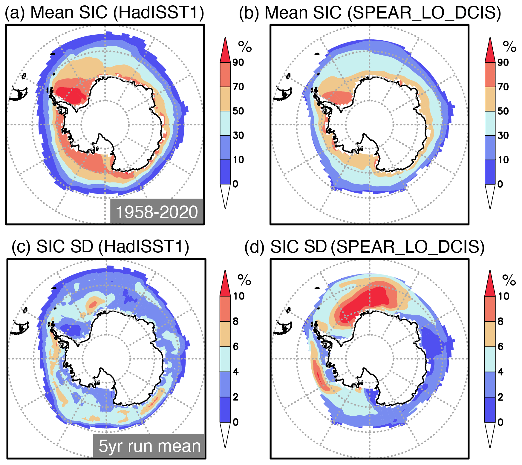
Figure 1(a) Annual mean sea ice concentration (SIC in %) observed during 1958–2020. (b) Same as in (a), but for the simulated SIC from the SPEAR_LO_DCIS. (c) Standard deviation of 5-year running mean SIC (in %) observed during 1958–2020. (d) Same as in (c), but for the simulated SIC from the SPEAR_LO_DCIS.
3.1 Antarctic sea ice multidecadal variability simulated in the SPEAR_LO Model
We show in Fig. 1 the annual mean SIC from HadISST1 and SPEAR_LO_DCIS. The observation (Fig. 1a) shows high SIC above 70 % in the Pacific and Atlantic sectors during 1958–2020. The SPEAR_LO_DCIS (Fig. 1b) captures the high SIC in these two regions, although the simulated SIC is somewhat lower than the observed SIC. Since the monthly climatology of the Antarctic SIE during austral summer for the SPEAR_LO_DCIS (Fig. S2) is lower than the observations, the underestimation of the annual mean SIC in the SPEAR_LO model is mostly due to that of the summertime SIC, which is also reported in other CGCMs contributing to the CMIP6 (Roach et al., 2020). We find a similar pattern for the satellite period of 1979–2020, although the monthly climatology of the Antarctic SIC during austral winter for the SPEAR_LO_DCIS is higher than that for NOAA/NSIDC (Fig. S2; see also Bushuk et al., 2021).
The standard deviation of 5-year running mean SIC anomalies from the observations (Fig. 1c) shows a large sea ice variability near the edge of sea ice in the Pacific sector and also near the coastal region of the eastern Weddell Sea. Here we employed a 5-year moving average of the monthly SIC anomalies to extract low-frequency variability with a period longer than 5 years. The large sea ice variability near the edge of sea ice in the Pacific sector is mostly due to that during austral autumn–spring (Fig. S3c, e, g), while the large sea ice variability in the coastal region of the eastern Weddell Sea is attributed to that during austral spring–autumn (Fig. S3a, c, g). This represents seasonal differences in the decadal sea ice variability over different regions. The SPEAR_LO_DCIS (Fig. 1d) also exhibits a large sea ice variability in these two regions, but the simulated SIC variability is much larger in the Weddell Sea. This is mostly due to the larger SIC variability simulated in the eastern Weddell Sea during austral winter and spring (Fig. S3f, h), although the SPEAR_LO_DCIS tends to capture the observed SIC variability there during austral summer and autumn (Fig. S3b, d).
In the coastal region of the eastern Weddell Sea, successive polynya events occurred during the austral winter of 1974–1976 (Carsey, 1980). The Weddell Polynya are generated through various processes (Morales Maqueda et al., 2004) such as the upwelling of deep warm water as a result of salinity-driven vertical convection (Martinson et al., 1981) and wind-driven sea ice divergence (Goosse and Fichefet, 2001). Two polynya events were recently reported during 2016–2017, partly contributing to the record-low sea ice in the Weddell Sea (Turner et al., 2020). A weaker ocean stratification and increased ocean eddy activities are suggested to provide favorable conditions for these polynya events (Cheon and Gordon, 2019), although synoptic atmospheric variability such as polar cyclones and atmospheric rivers may trigger these events (Francis et al., 2019, 2020). We find that the SPEAR_LO_DCIS captures the negative SIC anomalies associated with these polynya events in the eastern Weddell Sea during 1974–1976 (Fig. S4a, b). SPEAR_LO_DCIS also captures the negative peak of SIC anomalies near the coast of 0∘ E during 2016–2017 (Fig. S4c, d), but our model simulates the peak slightly equatorward with a weaker amplitude than the observation. It is difficult to attribute the 1974–1976 polynya events only to the large sea ice variability there. There are other reasons for the large sea ice variation in the eastern Weddell Sea of the SPEAR_LO_DCIS, which will be discussed later.
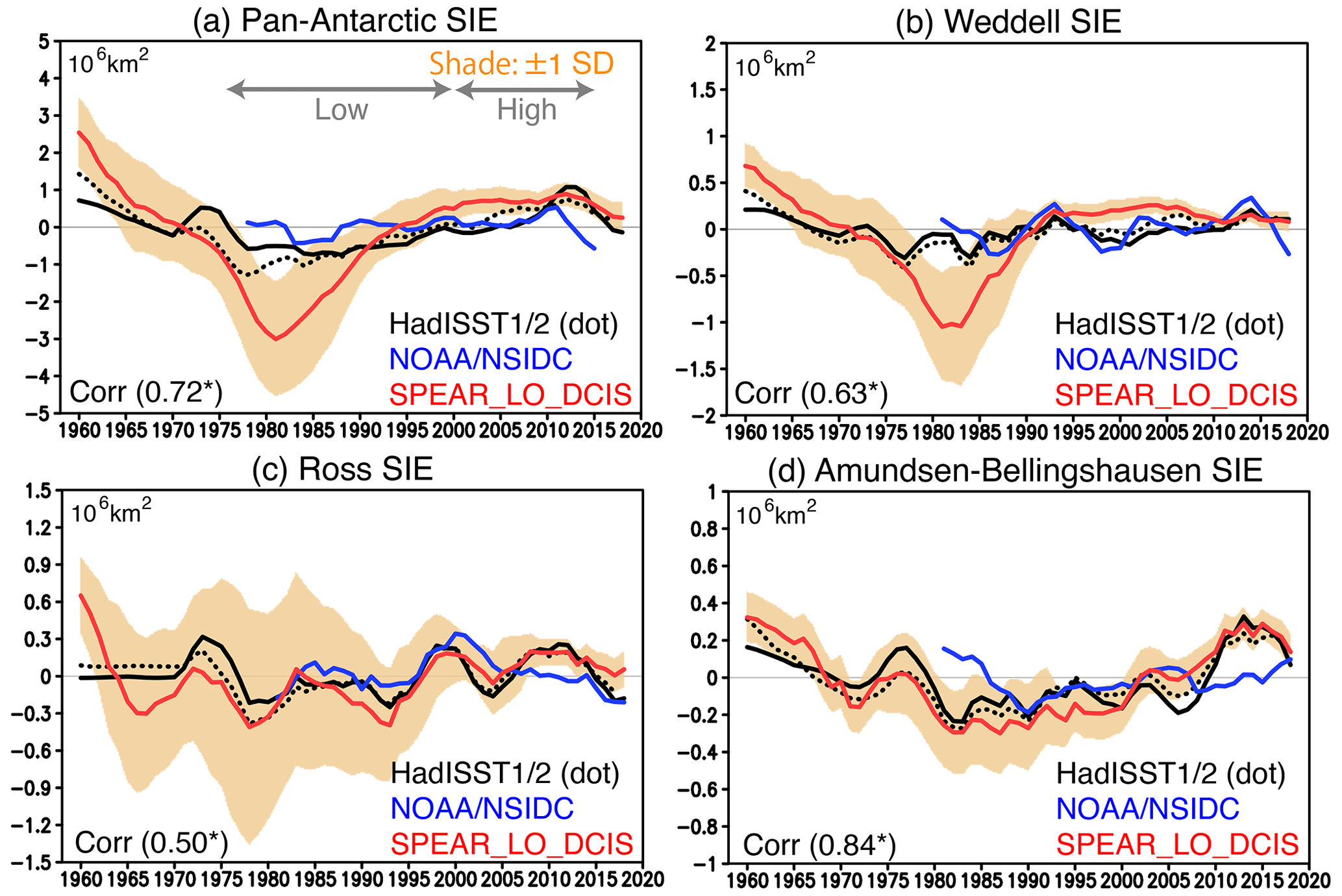
Figure 2(a) Time series of 5-year running mean sea ice extent (SIE in 106 km2) anomalies in the pan-Antarctic region during 1958–2020. Observations from HadISST1 (black solid), HadISST2 (black dotted), and the NOAA/NSIDC (blue) are shown, whereas the SPEAR_LO_DCIS is shown with a red line. Orange shades indicate 1 and −1 standard deviations of the SIE anomalies simulated from 30 ensemble members of SPEAR_LO_DCIS. Gray arrows correspond to a low sea ice period (late 1970s–1990s) and a high sea ice period (2000s–early 2010s). Correlation coefficient between HadISST1 and the SPEAR_LO_DCIS is shown in the bottom left where the asterisk indicates the statistically significant correlation at 90 % confidence level using Student's t test. (b–d) Same as in (a), but for the SIE anomalies in the Weddell Sea (60∘ W–0∘), Ross Sea (180–120∘ W), and Amundsen–Bellingshausen seas (120–60∘ W), respectively.
Time series of the pan-Antarctic SIE anomalies from the observations (Fig. 2a) show multidecadal variability with a low sea ice state (late 1970s–1990s) and a high sea ice state (2000s–early 2010s). A high sea ice state before the early 1970s is also reported in several studies, including the ones using the satellite images of Nimbus 1 and 2 in the 1960s (Meier et al., 2013; Gagné et al., 2015), data of sea ice edge latitude from the past 200 year reconstructed by ice core and fast-ice records (J. Yang et al., 2021), and a century-long SIE dataset reconstructed by major climate indices (Fogt et al., 2022). However, there is a large degree of uncertainty in the sea ice data before the satellite period. The SPEAR_LO_DCIS exhibits a similar multidecadal variability and has a significantly high correlation (0.72) with the observed SIE anomalies from HadISST1. Here we used 12 degrees of freedom to evaluate the statistical significance of the correlation coefficient because we applied a 5-year running mean filter to 63-year-long data. The model overestimates negative SIE anomalies between the late 1970s and early 1980s (Fig. 2a). This is mostly due to the model overestimation of negative SIE anomalies in the Weddell Sea (Fig. 2b), and the correlation value with HadISST1 is statistically significant (0.63) – slightly lower than that for the pan-Antarctic SIE. This can also be inferred from the model bias in capturing the large SIC variability in the Weddell Sea (Fig. 1d).
Since the ensemble spreads of the negative SIE anomalies are large, some members (5 out of 30 members) in the SPEAR_LO_DCIS are found to produce more reasonable SIE anomalies over the pan-Antarctic and Weddell Sea than in the observation (Fig. 2a, b). The ensemble spreads seem to decrease after the late 1990s when the sea ice starts to increase (Fig. 2b). The model simulation is constrained by the atmospheric and SST initializations but not by subsurface ocean data assimilation, so the larger ensemble spread in the early periods may be related to that in the ocean model, which will be discussed later. Other Antarctic seas such as the Ross and Amundsen–Bellingshausen seas also show a good agreement of the SIE anomalies between HadISST1 and SPEAR_LO_DCIS with significant correlations of 0.50 and 0.84, respectively (Fig. 2c, d). It should be noted that HadISST1 shows larger negative SIE anomalies in the Amundsen–Bellingshausen seas between 1980–1985 and larger positive SIE anomalies after 2010 than NOAA/NSIDC (Fig. 2d). This may be related to the SIC reconstruction of HadISST1 that uses different sea ice datasets (US National Ice Center, NASA, and the National Centers for Environmental Prediction – NCEP) before and after the mid-1990s which tend to show higher SIE in the latter period (Rayner et al., 2003).
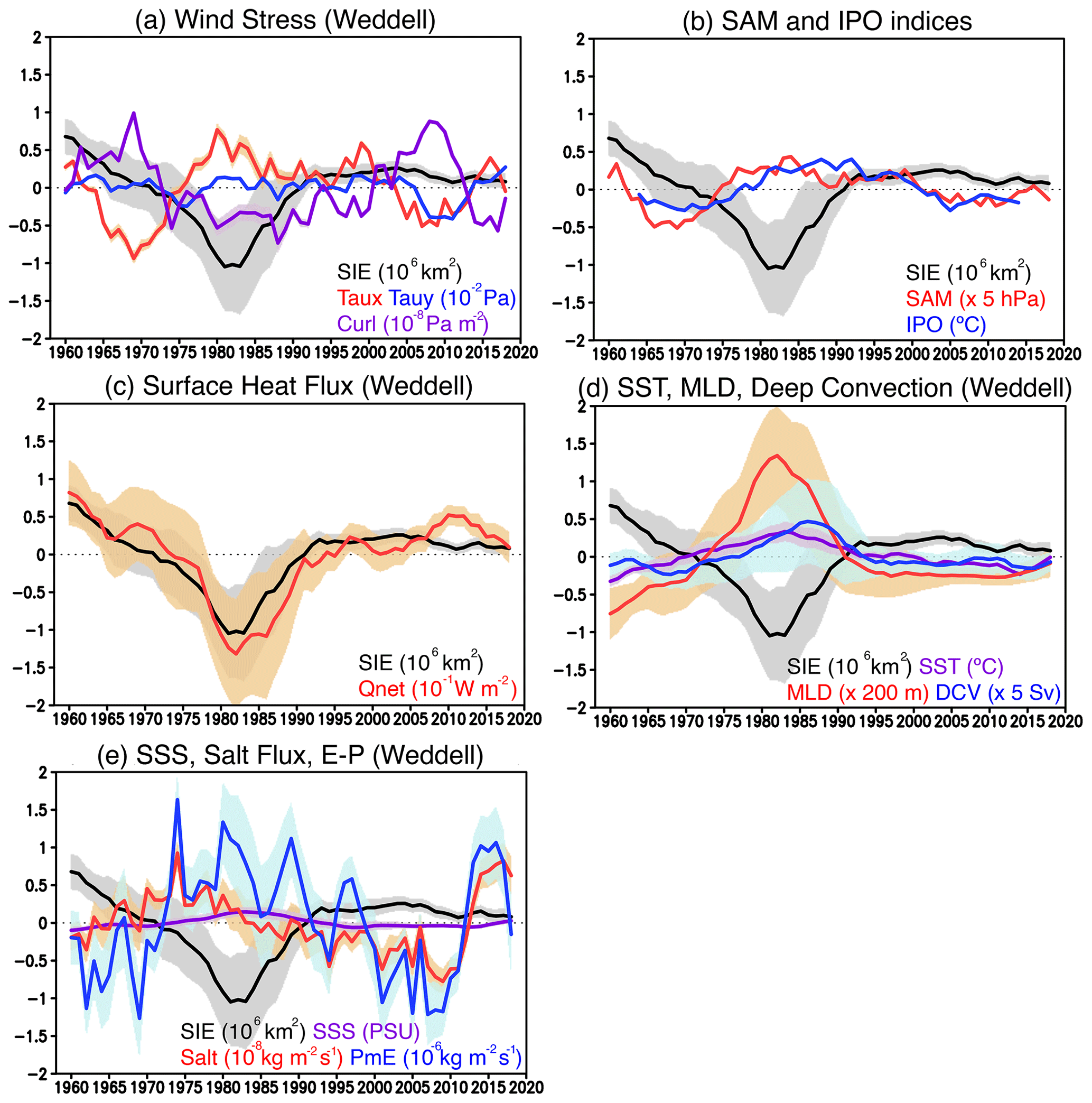
Figure 3(a) Time series of 5-year running mean SIE (black line in 106 km2), zonal (Taux; red in 10−2 Pa) and meridional (Tauy; blue in 10−2 Pa) wind stress, and wind stress curl (Curl; purple in 10−8 Pa m−2) anomalies averaged in the Weddell Sea (60∘ W–0∘, south of 55∘ S) during 1958–2020. Shades indicate 1 and −1 standard deviations of the anomalies from 30 ensemble members of the SPEAR_LO_DCIS. Positive wind stress curl anomalies correspond to downwelling anomalies in the ocean. (b) Same as in (a), but for the 5-year running mean SAM index (red in 5 hPa) and 13-year running mean IPO index (blue in ∘C). (c) Same as in (a), but for the SIE (black in 106 km2) and the net surface heat flux (Qnet; red in 10−1 W m−2) anomalies. Positive surface heat flux anomalies correspond to more heat going into the ocean. (d) Same as in (a), but for the SIE (black in 106 km2), sea surface temperature (SST; purple in ∘C), mixed-layer-depth (MLD; red in 200 m), and deep convection (DCV; blue in 5 Sv) anomalies. (e) Same as in (a), but for the SIE (black in 106 km2), sea surface salinity (SSS; purple in psu), salt flux (Salt; red in 10−8 kg m−2 s−1), and precipitation minus evaporation (PmE; blue in 10−6 kg m−2 s−1) anomalies. Positive salt flux anomalies correspond to anomalous salt going into the ocean at the surface associated with sea ice formation, whereas the positive PmE anomalies mean more freshwater going into the ocean.
3.2 Physical processes on the simulated Antarctic sea ice multidecadal variability
To explore physical mechanisms underlying the Antarctic sea ice multidecadal variability in the SPEAR_LO_DCIS, we focus on the Weddell Sea (60∘ W–0∘, south of 55∘ S), which contributes the most to the total sea ice variability in the SPEAR_LO_DCIS (Fig. 2a, b). Time series of 5-year running mean wind stress and curl anomalies (Fig. 3a) show that a significant SIE decrease between the late 1970s and early 1980s is associated with stronger westerlies and negative wind stress curl anomalies. These surface wind anomalies tend to induce anomalous upwelling of warm water from the subsurface ocean on decadal and longer timescales (Ferreira et al., 2015), contributing to the sea ice decrease. The westerly and negative curl anomalies coincide with a positive phase of the SAM (Fig. 3b), although ensemble spreads of the SAM index (Gong and Wang, 1999) are relatively large except for some periods (early 1960s, late 1970s, and early 1990s). The IPO index (Fig. 3b), which is defined as the 13-year running mean of the SST tripole index in the tropics and subtropics (Henley et al., 2015), is negative around 1975 when the westerly and negative curl anomalies start to appear, but it turns to positive values after 1980. This out-of-phase relationship indicates that the surface wind variability in the Weddell Sea is more related to the SAM than the IPO. On the other hand, the net surface heat flux (Fig. 3c) shows negative (upward) anomalies between the late 1970s and early 1980s. As a result of the decrease in sea ice, more heat is released from the ocean surface. We obtain an opposite but similar process for the high sea ice state after the 2000s when weaker westerlies and positive wind stress curl anomalies appear. These wind anomalies are found to have almost the same amplitude as those in the low sea ice period. This implies that the surface wind variability contributes to a part of the large negative SIE anomalies through shallower mixed-layer depths but does not necessarily explain all of the large negative SIE anomalies in the SPEAR_LO_DCIS during the late 1970s and early 1980s.
The substantial SIE decrease between the late 1970s and the early 1980s is associated with positive SST anomalies (Fig. 3d). A positive peak of the SST anomalies in the early 1980s is associated with a positive peak of the mixed-layer-depth anomalies followed by that of the deep convection anomalies. The deepening of the mixed layer and the associated deep convection tend to entrain more warm water from the subsurface ocean. This plays a crucial role in the development of extremely low sea ice in the Weddell Sea. Moreover, the negative SIE anomalies are accompanied by positive sea surface salinity (SSS) anomalies (Fig. 3e). Net salt flux into the ocean at the surface associated with sea ice formation shows positive anomalies, but the amplitude is much smaller than for positive anomalies of the precipitation minus evaporation corresponding to net surface water flux into the ocean. As a result of the decrease in sea ice, more freshwater goes into the ocean, but this cannot explain the SSS increase in the Weddell Sea. Rather, the SSS increase is driven by other processes such as the deeper mixed layer associated with the surface wind variability and the deep convection that entrain relatively high-salinity water from the subsurface ocean.
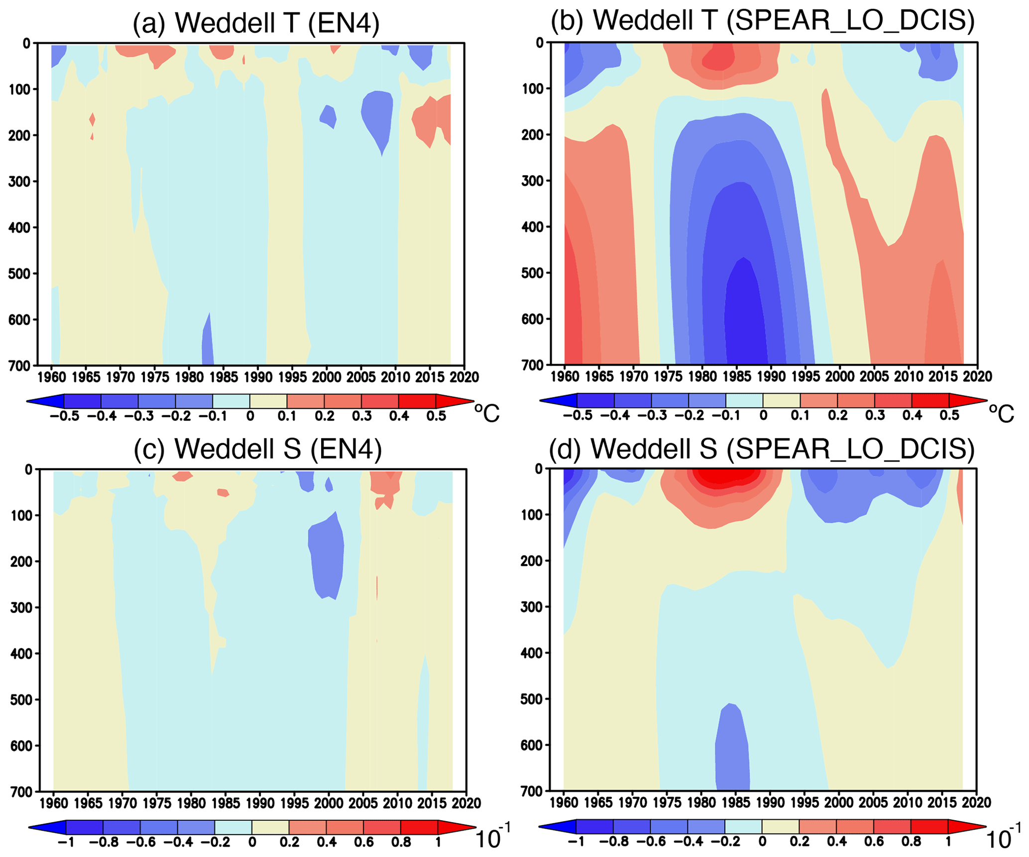
Figure 4(a) Temporal evolution of 5-year running mean ocean temperature (in ∘C) anomalies averaged in the Weddell Sea as a function of depth (in m). (b) Same as in (a), but for the ocean temperature anomalies simulated from the SPEAR_LO_DCIS. (c) Temporal evolution of ocean salinity (in 10−1 psu) anomalies averaged in the Weddell Sea as a function of depth (in m). (d) Same as in (a), but for the ocean salinity anomalies simulated from the SPEAR_LO_DCIS.
To highlight a possible role of subsurface ocean variability, we describe time series of ocean temperature and salinity anomalies averaged in the Weddell Sea as a function of depth (Fig. 4). Observation data (Fig. 4a) show that sea ice decrease between the late 1970s and early 1980s was accompanied by positive temperature anomalies in the upper 200 m and negative temperature anomalies below 200 m. The SPEAR_LO_DCIS (Fig. 4b) captures this dipole structure of the positive and negative temperature anomalies, although the amplitude is much larger than that in the observations. Interestingly, both the observations and SPEAR_LO_DCIS (Fig. 4a, b) show that the positive temperature anomalies in the upper 200 m start to appear in the early 1970s and are preceded by positive temperature anomalies below 200 m in the 1960s, although the SPEAR_LO_DCIS has uncertainty in simulations of the subsurface temperature anomalies in the Weddell Sea during the early 1960s because of the slow oceanic response to the prescribed atmospheric forcing since 1958. The anomalous heat buildup in the subsurface ocean during the 1960s may have links to the subsequent surface warming in the 1970s. On the other hand, the salinity anomalies between the late 1970s and the early 1980s are positive in the upper 200 m and negative below 200 m for both the observation (Fig. 4c) and SPEAR_LO_DCIS (Fig. 4d). Since both the temperature and salinity anomalies exhibit the dipole structure in the vertical, vertical ocean processes are expected to be in operation to induce these anomalies.
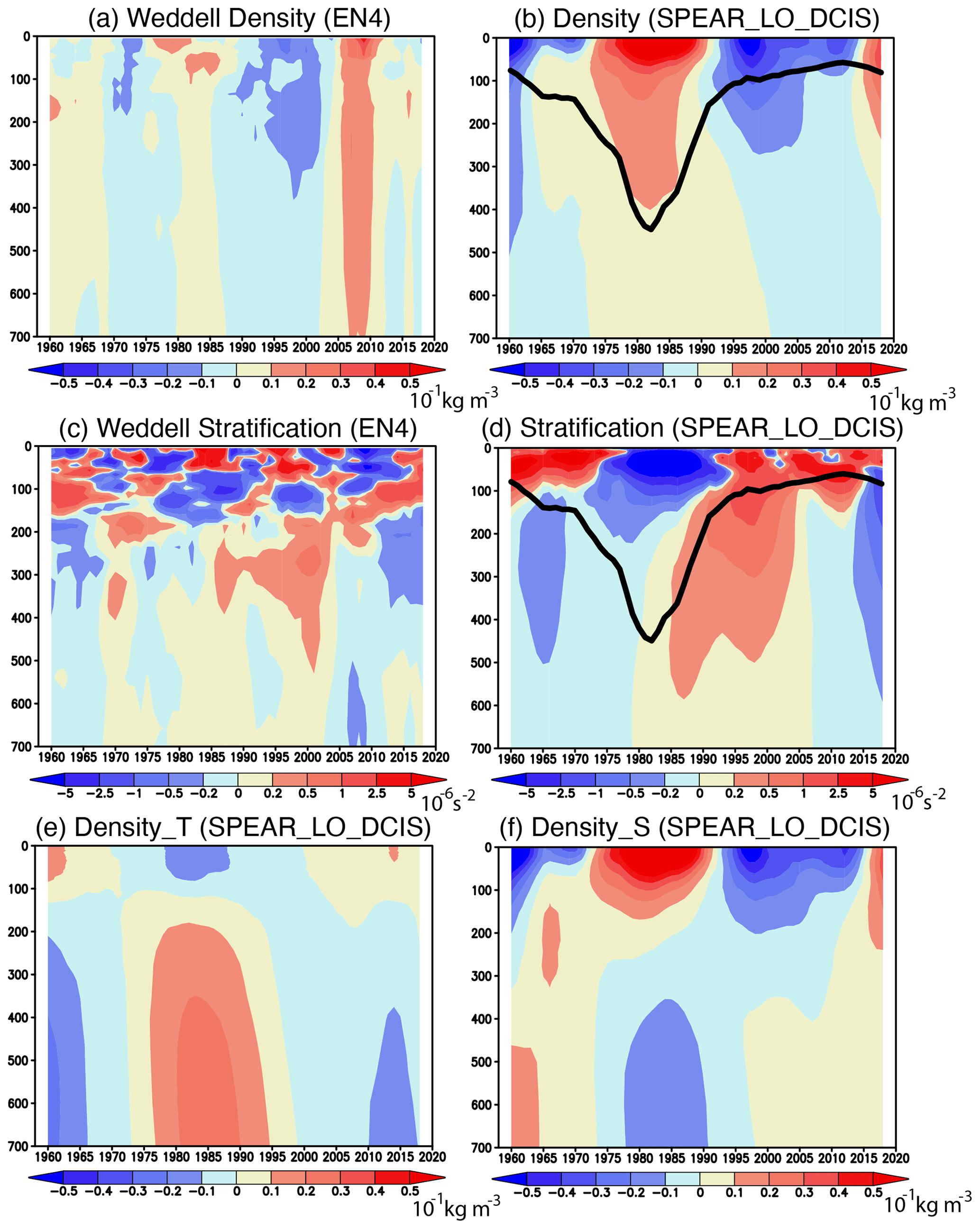
Figure 5(a) Temporal evolution of 5-year running mean ocean density anomalies (in 10−1 kg m−3) averaged in the Weddell Sea from the EN4 as a function of depth (in m). (b) Same as in (a), but for the SPEAR_LO_DCIS. A black line indicates a mixed-layer depth at which the ocean density increases by 0.03 kg m−3 from the one at the ocean surface. (c) Same as in (a), but for the ocean stratification (squared Brunt–Väisälä frequency in 10−6 s−2) anomalies. Positive stratification anomalies indicate a higher stability of sea water. (d) Same as in (c), but for the SPEAR_LO_DCIS. A black line indicates a mixed-layer depth at which the ocean density increases by 0.03 kg m−3 from the one at the ocean surface. (e) Same as in (b), but for the ocean density anomalies (in 10−1 kg m−3) driven by the ocean temperature anomalies independent of the ocean salinity anomalies. (f) Same as in (b), but for the ocean density anomalies (in 10−1 kg m−3) driven by the ocean salinity anomalies independent of the ocean temperature anomalies.
The observed ocean density shows positive anomalies from the surface to the deeper ocean around 1980 (Fig. 5a). The SPEAR_LO_DCIS also shows the higher density around 1980, although the amplitude is larger than the observation (Fig. 5b). Associated with the positive density anomalies, the mixed layer anomalously deepens. The observed ocean stratification, which is estimated by squared Brunt–Väisälä frequency, shows negative anomalies in the upper 200 m around 1980 (Fig. 5c). The SPEAR_LO_DCIS also shows weaker stratification (Fig. 5d), which starts to appear below 100 m in the 1960s and provides favorable conditions for the deepening of the mixed layer. We decomposed the density anomalies into the anomalies solely dependent on temperature anomalies and other ones accompanied by salinity anomalies. We find that the negative density anomalies below 200 m in the 1960s are driven by the warm temperature anomalies (Figs. 4b, 5e), whereas the positive density anomalies in the upper 200 m during the late 1970s and early 1980s arise from those associated with the positive salinity anomalies (Figs. 4d, 5f). Both the subsurface heat buildup in the 1960s and the surface salinity increase linked to the surface wind variability in the 1970s (Fig. 3a) contribute to the deepening of the mixed layer from the 1960s to the early 1980s, which results in warmer SST and sea ice decrease.
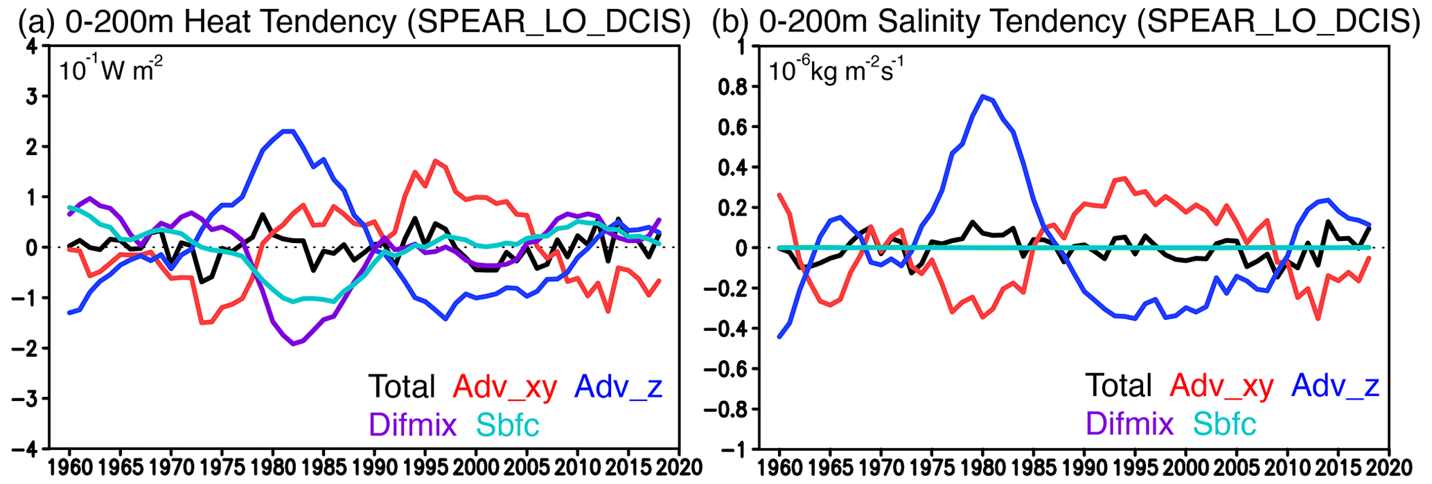
Figure 6(a) Time series of 5-year running mean ocean heat tendency (in 10−1 W m−2) anomalies in the upper 200 m of the Weddell Sea from the SPEAR_LO_DCIS. Total ocean heat tendency (Total; black), horizontal advection (Adv_xy; red), vertical advection (Adv_z; blue), mesoscale diffusion and dianeutral mixing (Difmix; purple), and surface boundary forcing (Sbfc; light blue) anomalies are shown. (b) Same as in (a), but for the salinity tendency (in 10−6 kg m−2 s−1) anomalies.
To further investigate how the surface temperature and salinity anomalies are generated, we evaluated ocean heat and salinity tendency anomalies in the upper 200 m (Fig. 6). Here we combine both contributions from the dianeutral mixing and mesoscale diffusion into one term because the contribution from the mesoscale diffusion is found to be much smaller than that from the dianeutral mixing. The heat tendency anomalies in the upper 200 m (Fig. 6a) are positive in the late 1970s and early 1980s when the positive SST and negative SIE anomalies develop (Fig. 3d). The positive heat tendency anomalies are mostly due to the vertical advection, although they are partly contributed by the vertical mixing and horizontal advection. Similarly, the positive salinity tendency anomalies in the upper 200 m during the period are mostly explained by the vertical advection. These results indicate that the deepening of the mixed layer (Fig. 3d) entrains more warm and saline water from below the mixed layer to increase the ocean temperature and salinity at the surface. We obtain a similar but opposite process for negative temperature tendency anomalies after the late 1990s when the positive SIE anomalies develop (Fig. 3d).
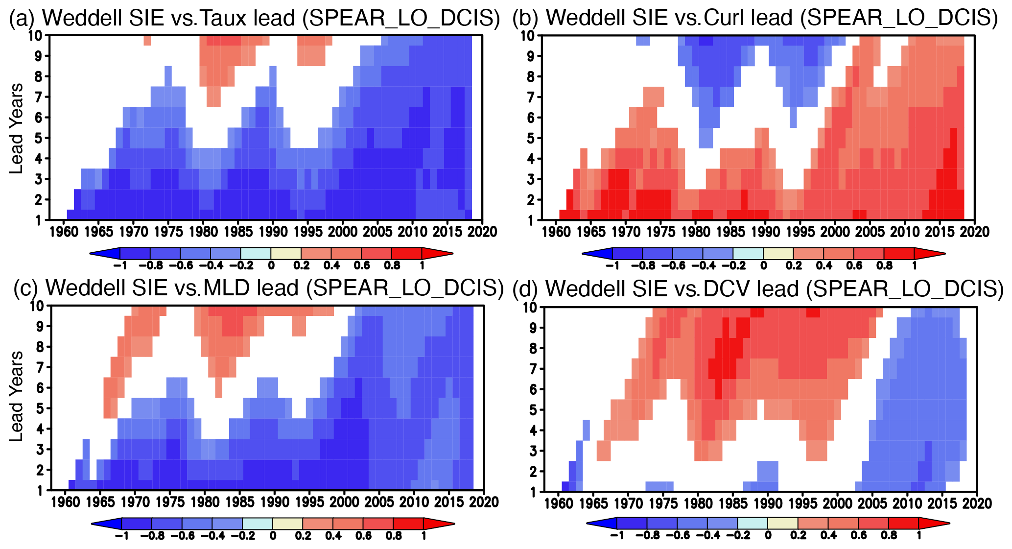
Figure 7(a) Temporal evolution of inter-member correlation between the 5-year running mean SIE anomalies and the 5-year running mean zonal wind stress (Taux) averaged in the Weddell Sea from 30 ensemble members of the SPEAR_LO_DCIS as a function of lead years (y axis). Positive lead years mean that the Taux anomalies lead the SIE anomalies by the number of years. Correlation coefficients that are statistically significant at 90 % using Student's t test are shown in color. (b) Same as in (a), but for the inter-member correlation between the SIE anomalies and the wind stress curl (Curl) anomalies. (c) Same as in (a), but for the inter-member correlation between the SIE anomalies and the mixed-layer-depth (MLD) anomalies. (d) Same as in (a), but for the inter-member correlation between the SIE anomalies and the deep convection (DCV) anomalies.
3.3 Ensemble spreads of the simulated Antarctic sea ice multidecadal variability
We have so far discussed physical processes for ensemble mean fields of the SPEAR_LO_DCIS, but this analysis does not provide any explanation for the ensemble spreads representing model uncertainty. To explore the underlying causes of ensemble spreads in a simple way, we performed inter-member correlation analysis for 30 ensemble members of the SPEAR_LO_DCIS. Here we calculated the correlation between the anomalies of SIE and other variables simulated from the 30 ensemble members, assuming that initial differences in the anomalies of other variables lead to those in the SIE anomalies. Figure 7a shows time series of inter-member correlation coefficients between the 5-year running mean SIE anomalies and the leading zonal wind stress anomalies in the Weddell Sea as a function of lead years. Zonal wind stress anomalies have significantly large negative correlations with SIE anomalies by 3–4 lead years during the 1970s and the 1980s when the sea ice anomalously decreases. This means that ensemble members with stronger westerlies than the ensemble mean tend to simulate a larger sea ice decrease 3–4 years later. We find weakly positive correlations around the 1980s with lead times longer than 6 years, but these cannot explain the sea ice decrease because the weaker westerlies tend to suppress the upwelling of warm water from the subsurface and contribute to sea ice increase. Rather, this can be interpreted as the decadal changes in the phase of zonal wind anomalies from the 1970s to the 1980s (Fig. 3a) and may have nothing to do physically with the negative zonal wind anomalies in the 1970s. The negative correlations with the zonal wind stress become stronger with longer lead times after the late 1990s when the sea ice anomalously increases. This represents more influence of weaker westerlies on the anomalous sea ice increase. We obtain similar but opposite correlations between the SIE anomalies and the leading wind stress curl anomalies (Fig. 7b). Ensemble members with more negative wind stress curl anomalies than the ensemble mean tend to simulate a larger sea ice decrease in the 1970s and the 1980s and vice versa after the late 1990s.
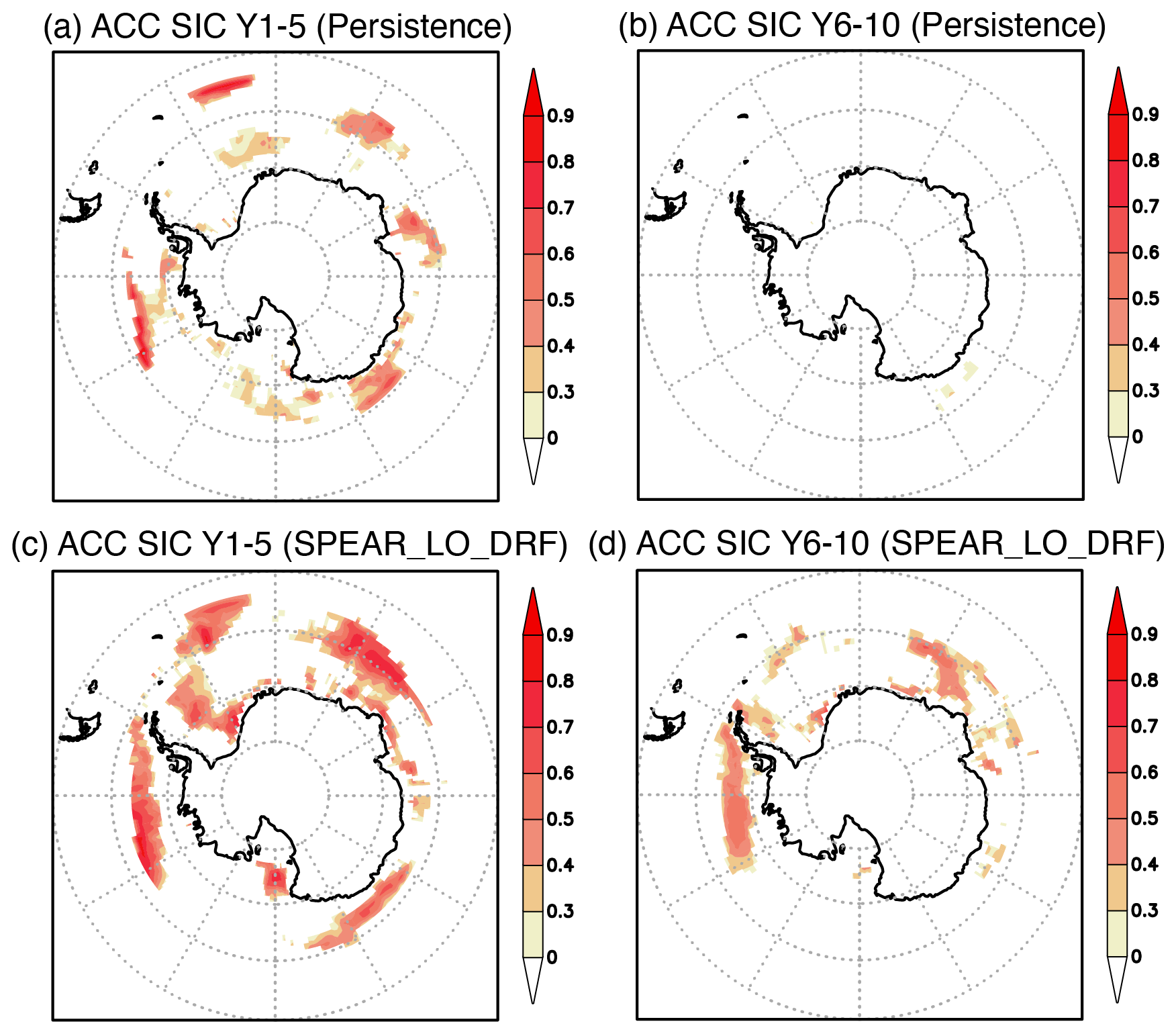
Figure 8(a) Anomaly correlation (ACC) of the SIC anomalies from the persistence prediction at a lead time of 1–5 years. Positive ACCs that are statistically significant at 90 % using Student's t test are colored. (b) Same as in (a), but for the ACC from the persistence prediction at a lead time of 6–10 years. (c) Same as in (a), but for the ACC between the observed SIC anomalies and the ensemble mean SIC anomalies predicted at a lead time of 1–5 years in the SPEAR_LO_DRF. (d) Same as in (c), but for the ACCs of the ensemble mean SIC anomalies predicted at a lead time of 6–10 years in the SPEAR_LO_DRF.
Inter-member correlations between the SIE anomalies and the leading mixed-layer-depth (MLD) anomalies (Fig. 7c) show significantly large and negative values by 3–4 lead years in the 1970s and the 1980s and by 5–6 lead years after the late 1990s. This indicates that ensemble members with a deeper mixed layer than the ensemble mean tend to simulate a larger sea ice decrease 3–4 years later in the 1970s and the 1980s, whereas the members with a shallower mixed layer than the ensemble mean tend to simulate a larger sea ice increase 5–6 years later after the late 1990s. It should be noted that we used spatially averaged values over the whole Weddell Sea (60∘ W–0∘), so the results also include the destratified process near the coast dominated by sea ice production. However, the SIE variability in the Weddell Sea is pronounced in the open water (Fig. 1d), so the results mostly represent the open-water stratified process of cold and fresh water over warm and salty circumpolar deep water. Similarly, we find negative correlations between the SIE anomalies and the 1–2-year leading deep convection anomalies (Fig. 7d), but the links with the deep convection are much weaker than the mixed layer. We also find positive correlations with the 5–10-year leading deep convection anomalies, but this can also be interpreted as decadal changes in the phase of deep convection anomalies (Fig. 3d) and may have nothing to do physically with deep convection anomalies in the earlier period. Therefore, the large uncertainty in the simulated amplitude of the mixed layer contributes more to that in the sea ice decrease in the late 1970s and 1980s, while the model uncertainty in the surface wind variability contributes more to that in the sea ice increase after the late 1990s (Fig. 7a–c).
3.4 Skillful prediction of Antarctic sea ice multidecadal variability
For the quantitative assessment of prediction skills of the Antarctic sea ice multidecadal variability, we first calculated anomaly correlations (ACCs) of the 5-year mean SIC anomalies for the persistence prediction using the observed SIC anomalies from HadISST1 (Fig. 8a, b). Here we used 50 degrees of freedom to evaluate the statistical significance of the ACC because we performed decadal reforecasts independently starting from each year of 1961–2011. Persistence prediction shows very limited prediction skills of the sea ice variability in the Antarctic seas at a lead time of 1–5 years (Fig. 8a). The ACCs significantly drop below zero at a lead time of 6–10 years (Fig. 8b), indicating that the observed SIC anomalies cannot persist beyond 5 years. This can also be seen in the year-to-year ACCs (Fig. S5) that show the highest values in lead year 1, quickly decay in lead year 2, and then vanish afterward.
To compare with the persistence prediction skills, we calculated the ACCs between the 5-year mean observed SIC anomalies and the ensemble mean (i.e., simple average of 20 members) of the predicted SIC anomalies from the SPEAR_LO_DRF for the prediction lead times of 1–5 and 6–10 years, separately (Fig. 8c, d). For example, in the case of 1–5-year lead prediction for the targeted observation period of 2010–2014, we used the predicted anomalies starting from 2005–2009 to 2009–2013. The ACCs in the SPEAR_LO_DRF are significantly high at a lead time of 1–5 years (Fig. 8c) compared to the persistence prediction (Fig. 8a). In particular, the ACCs become higher in the Amundsen–Bellingshausen seas, Weddell Sea, and Indian sector. These regions correspond well to those with higher ACCs of the SST in the model (see Fig. 10 in X. Yang et al., 2021), indicating a close relationship between the SIC and SST variations. The ACCs in these regions become smaller but remain significant for a lead time of 6–10 years (Fig. 8d).
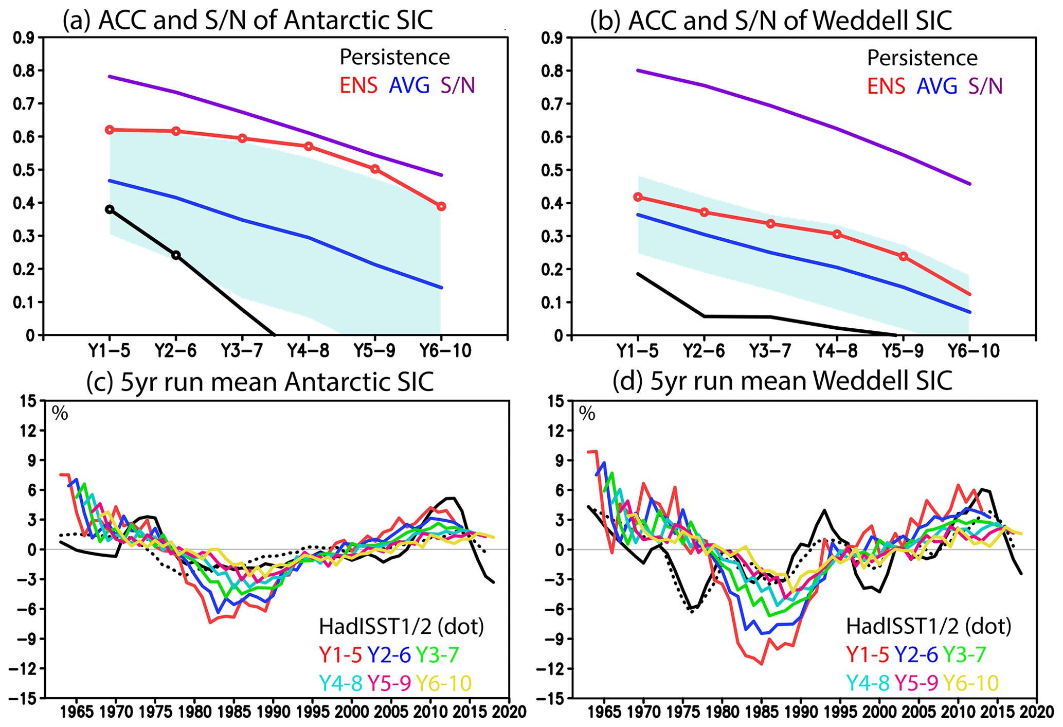
Figure 9(a) ACC and signal-to-noise () ratio of pan-Antarctic (area-weighted mean) SIC anomalies predicted at lead times from 1–5 to 6–10 years. The ACCs from the persistence prediction (black) and the SPEAR_LO_DRF ensemble mean (ENS; red), which are statistically significant at 90 % confidence level using Student's t test, are described with open circles. The average (AVG; blue) of individual ACCs from the SPEAR_LO_DRF is shown with its 1 standard deviation (shade in light blue). The ratio from the SPEAR_LO_DRF (purple) is also plotted. (b) Same as in (a), but for the ACC and ratio of the SIC anomalies averaged in the Weddell Sea. (c) Time series of 5-year running mean pan-Antarctic SIC (in %) anomalies during 1961–2020. Black lines show the observed SIC anomalies from HadISST1 (solid) and HadISST2 (dotted), whereas other colored lines correspond to the ensemble mean SIC anomalies predicted at lead times from 1–5 to 6–10 years in the SPEAR_LO_DRF. (d) Same as in (c), but for the SIC anomalies averaged in the Weddell Sea.
The high ACCs at a lead time of 1–5 years are mostly due to those during austral autumn–spring (Fig. S6c, e, g), while the significant ACCs at a lead time of 6–10 years are mainly attributed to those during austral winter and spring (Fig. S5f, h). Decadal sea ice predictability during austral summer (Fig. S6a, b) is the lowest because the sea ice extent reaches its minimum and the decadal SIC variability is confined near the Antarctic coast occupying smaller areas (Fig. S3a). We can also find that the year-to-year prediction skills of the ACC from the SPEAR_LO_DRF (Fig. S7) are higher than those from the persistence prediction (Fig. S5), although the amplitude of the ACC (Fig. S7) is lower than the prediction skills of 5-year mean SIC (Fig. 8c, d) probably due to large interannual variations of the Antarctic SIC.
To further demonstrate the spatiotemporal evolution of prediction skills in the SPEAR_LO_DRF, we calculated the ACCs of the 5-year area-weighed mean SIC anomalies in the pan-Antarctic region and the Weddell Sea as a function of lead times (Fig. 9a, b). The ACCs of the pan-Antarctic SIC anomalies in the SPEAR_LO_DRF are significantly higher than those in the persistence prediction for any lead time from 1–5 to 6–10 years (Fig. 9a). A few ensemble members have low ACCs comparable to the persistence prediction, but the ACCs of the ensemble mean SIC anomalies are high at around 0.4–0.6. We also find that the ACCs are relatively high compared to the average of the individual ACCs. The ratio in the model also exceeds the ACCs of the ensemble mean. These results indicate that the model prediction is under-dispersive and overconfident. We obtain similar results for the ACCs of the SIC anomalies in the Weddell Sea (Fig. 9b), but the ACCs become insignificant after a lead time of 6–10 years. Overall, the ACCs in the Weddell Sea are lower than those in the pan-Antarctic region.
Since the ACCs do not evaluate skills for the amplitude of the predicted anomalies, we plotted time series of the 5-year running mean SIC anomalies in the pan-Antarctic region and the Weddell Sea for different lead times from 1–5 to 6–10 years (Fig. 9c, d). The SPEAR_LO_DRF better captures the observed SIC anomalies in the pan-Antarctic region than the Weddell Sea (Fig. 9c, d). As the lead times increase, the amplitude of the predicted anomalies decreases and gets closer to the observation, particularly during the 1980s (Fig. 9c, d). Since the time series of the predicted anomalies for the 1–5-year leads resembles that of the initial sea ice anomalies in the model (Fig. 2a, b), the influence of the Southern Ocean deep convection initialized in the model during the 1980s remains stronger for the earlier lead times, as will be discussed below, causing larger differences in the observed and predicted amplitudes. The predicted SIC anomalies return to neutral at around 2000 and become positive afterwards, although the model underestimates the positive SIC anomalies observed in the early 2010s. We find similar results for the Antarctic SIC anomalies normalized by standard deviation, but the predicted amplitude gets closer to the observation (Fig. S8a). For the SIC anomalies in the Weddell Sea (Figs. 9d, S8b), the observed anomalies largely fluctuate on a shorter timescale, so the model cannot capture positive SIC anomalies in the early 1990s and negative SIC anomalies in the mid-1970s and late 1990s.
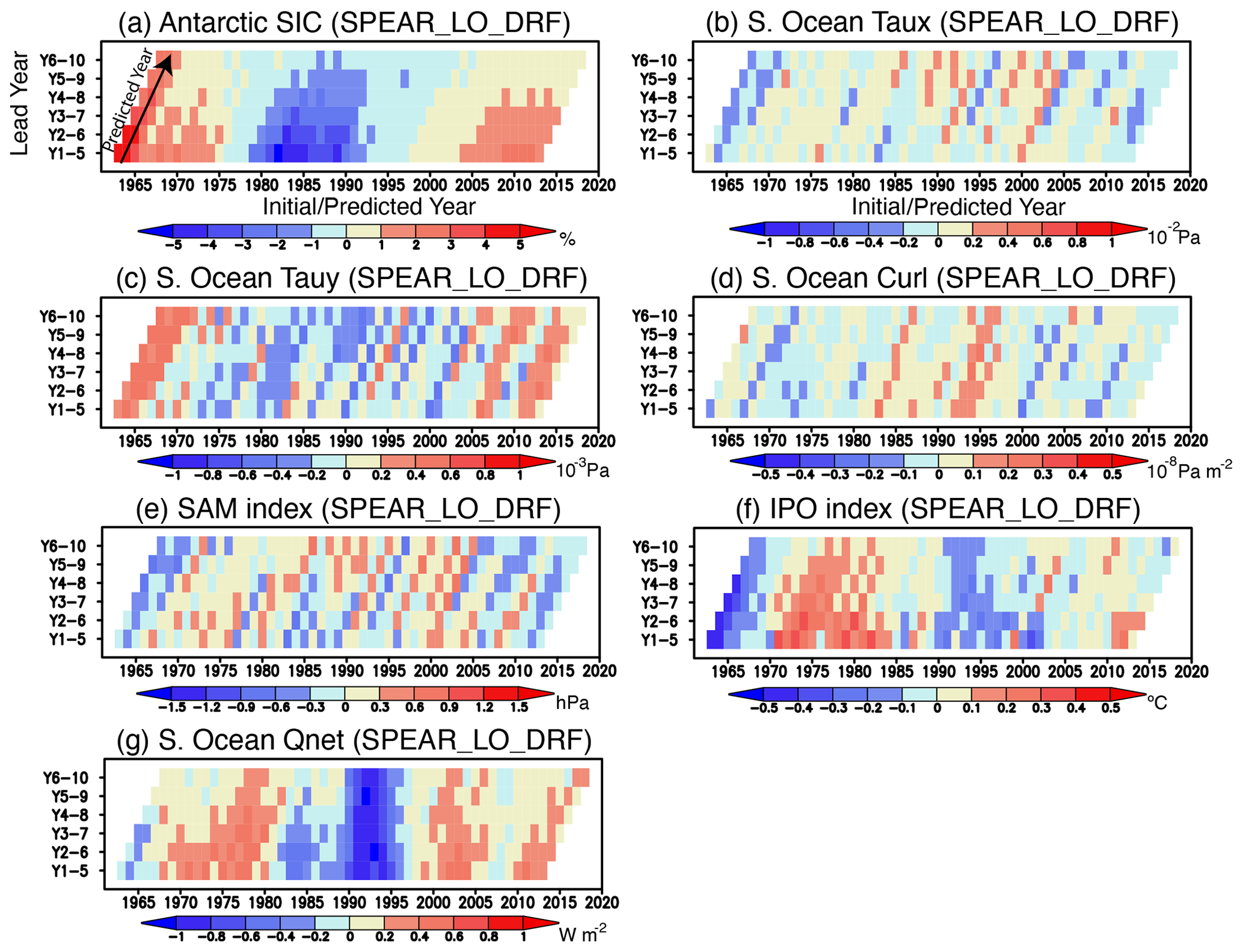
Figure 10(a) Temporal evolution of ensemble mean pan-Antarctic SIC anomalies predicted at lead times from 1–5 to 6–10 years in the SPEAR_LO_DRF as a function of initial/predicted years (x axis) and lead years (y axis). A black arrow indicates the correlations with the same initial year for different lead times, while the corresponding x axis indicates the predicted years. (b–d) Same as in (a), but for the zonal wind stress (Taux; 10−2 Pa), meridional wind stress (Tauy; 10−3 Pa), and wind stress curl (Curl; 10−8 Pa m−2) anomalies averaged in the Southern Ocean (south of 55∘ S). Positive wind stress curl anomalies correspond to downwelling anomalies in the ocean. (e–f) Same as in (a), but for the SAM (in hPa) and IPO (in ∘C) indices, respectively. (g) Same as in (b), but for the net surface heat flux anomalies (in W m−2). Positive surface heat flux anomalies indicate more heat going into the ocean.
3.5 Potential sources of Antarctic sea ice multidecadal predictability
The temporal evolution of the pan-Antarctic SIC anomalies in the SPEAR_LO_DRF (Fig. 10a) shows that positive and negative SIC anomalies predicted at a lead time of 1–5 years tend to persist over 5 years up to a lead time of 6–10 years. Negative SIC anomalies predicted in the 1980s for a lead time of 1–5 years gradually weaken as the lead time increases but remain the same in the late 1980s and early 1990s for a lead time of 6–10 years. The negative SIC anomalies in the late 1980s and early 1990s for a lead time of 6–10 years are associated with positive zonal wind anomalies and negative meridional wind anomalies (Fig. 10b, c). The stronger westerlies act to induce northward Ekman current anomalies on interannual and shorter timescales, but on decadal and longer timescales, the associated upwelling of warm water from the subsurface ocean tends to reduce the SIC (Ferreira et al., 2015). Also, the northerly anomalies contribute to the SIC decrease by bringing more warm air from the north during the period. The wind stress curl (Fig. 10d) shows positive anomalies in the 1980s for a lead time of 1–5 years and also in the late 1980s and early 1990s for a lead time of 6–10 years. However, the positive wind stress curl anomalies tend to weaken the upwelling of warm water from the subsurface ocean and decrease the upper-ocean temperature. This is inconsistent with sea ice decrease during that period.
The westerly anomalies in the late 1980s and early 1990s for a lead time of 6–10 years are associated with a positive phase of the SAM (Fig. 10e), while the IPO index changes from the positive to negative values (Fig. 10f). The closer link of the surface wind variability with the SAM is consistent with the previous discussion in the Weddell Sea (Fig. 3b). The net surface heat flux (Fig. 10g) also shows negative anomalies in the 1980s and early 1990s for all lead times. This represents more heat release from the ocean surface as a result of the sea ice decrease. We obtain similar but opposite processes for the positive SIC anomalies after the 2000s.
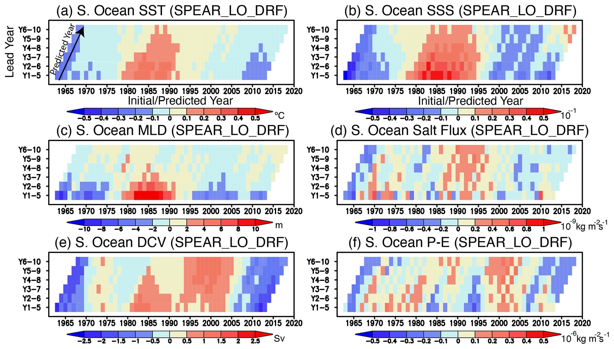
Figure 11(a) Temporal evolution of ensemble mean Southern Ocean (south of 55∘ S) SST anomalies predicted at lead times from 1–5 to 6–10 years in the SPEAR_LO_DRF as a function of initial/predicted years (x axis) and lead years (y axis). A black arrow indicates the correlations with the same initial year for different lead times, while the corresponding x axis indicates the predicted years. (b–f) Same as in (a), but for the SSS (in 10−1 psu), mixed-layer-depth (MLD; in m), salt flux (in 10−9 kg m−2 s−1), deep convection (DCV; in Sv), and precipitation minus evaporation (P−E; in 10−6 kg m−2 s−1) anomalies averaged in the Southern Ocean, respectively.
To elucidate on a potential role of ocean variability, we plotted the temporal evolution of 5-year running mean anomalies of predicted ocean variables (Fig. 11). The Southern Ocean SST (Fig. 11a) shows positive anomalies in the 1980s for a lead time of 1–5 years and in the late 1980s and early 1990s for a lead time of 6–10 years. This represents the persistence of the predicted SST anomalies over 5 years. The positive SST anomalies are strongly accompanied by positive mixed-layer-depth anomalies in the 1980s (Fig. 11c) and positive deep convection anomalies in the late 1980s (Fig. 11e) for lead times between the 1–5 and 3–7 years. As explained earlier, the deepening of the mixed layer and the associated deep convection contribute to the positive SST anomalies by entraining warm water from the subsurface ocean into the surface mixed layer.
During that period, SSS anomalies (Fig. 11b) are positive in association with the slightly positive anomalies of the net salt flux into the ocean (Fig. 11d). Precipitation minus evaporation corresponding to the net surface water flux into the ocean (Fig. 11f) shows slightly negative anomalies. This represents more evaporation from the ocean surface as a result of sea ice decrease. Given that the amplitude of the freshwater flux anomalies is much larger than the salt flux anomalies, the evaporation from the ocean surface contributes partly to the SSS increase in the 1980s. In addition to the effect of surface evaporation, the deepening of the mixed layer and the associated deep convection help increase the SSS during that period. We obtain similar but opposite processes for the sea ice increase after the 2000s. More freshwater input (Fig. 11f) and anomalous heat input (Fig. 10g) into the surface mixed layer may contribute to the shallower mixed layer. This indicates more active roles of atmosphere–ocean interaction at the surface than the subsurface ocean variability.
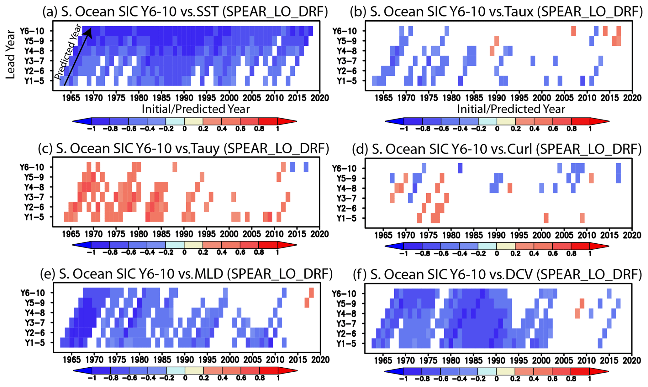
Figure 12(a) Temporal evolution of inter-member correlation between the pan-Antarctic SIC anomalies predicted at a lead time of 6–10 years and the Southern Ocean SST anomalies predicted at lead times from 1–5 to 6–10 years for the 20 ensemble members of the SPEAR_LO_DRF as a function of initial/predicted years (x axis) and lead years (y axis). A black arrow indicates the correlations with the same initial year for different lead times, while the corresponding x axis indicates the predicted years. Correlation coefficients that are statistically significant at 90 % confidence level using Student's t test are colored. (b–f) Same as in (a), but for the inter-member correlation with the zonal wind stress, meridional wind stress, wind stress curl, mixed-layer-depth, and deep convection anomalies averaged in the Southern Ocean.
To further examine possible links with atmosphere and ocean variability among ensemble members, we calculated the temporal evolution of inter-member correlations between the SIC anomalies for a lead time of 6–10 years and the SST anomalies for each lead time from 1–5 to 6–10 years (Fig. 12a). For example, the correlation coefficient in 1980 with a lead time of 1–5 years is the one between the SIC anomalies predicted in 1986–1990 and the SST anomalies predicted in 1981–1985. The SIC anomalies predicted at a lead time of 6–10 years show significantly negative correlations with the SST anomalies in the 1980s for a lead time of 1–5 years. This means that ensemble members with larger positive SST anomalies in the 1980s tend to predict larger negative SIC anomalies 5 years later. Zonal and meridional wind stress anomalies (Fig. 12b, c) show significantly negative and positive correlations with the SIC anomalies, respectively, as expected from the ensemble mean results (Fig. 10b, c). However, the links with the wind stress curl anomalies (Fig. 12d) are much weaker.
On the other hand, the mixed-layer-depth and deep convection anomalies in the 1980s (Fig. 12e, f) show significantly negative correlations with the SIC anomalies for a lead time of 6–10 years, although the deep convection shows a weaker correlation than the mixed-layer depth. This indicates that ensemble members with a deeper mixed layer and stronger deep convection than the ensemble mean tend to predict a larger sea ice decrease and vice versa. However, the links with deep convection become weaker after the 2000s when the sea ice anomalously increases. The correlation coefficients with zonal and meridional wind anomalies after the 2000s (Fig. 12b, c) are low but more significant than those with the deep convection anomalies (Fig. 12f). These results suggest that subsurface ocean variability contributes to skillful and long-lead-time prediction of sea ice decrease in the 1980s, while the surface wind variability contributes more to the skillful prediction of the sea ice variability than the deep convection after the 2000s.
This study has examined the relative importance of the Southern Ocean deep convection and surface winds in the Antarctic sea ice multidecadal variability and predictability using the GFDL SPEAR_LO model. Observed SIE anomalies show a multidecadal variability with a low sea ice state (late 1970s–1990s) and a high sea ice state (2000s–early 2010s). The trend of increasing SIE from the late 1990s to the early 2010s is reported in many studies (e.g., Yuan et al., 2017; Parkinson, 2019), and this is in contrast to a significant SIE decrease in the early and middle 20th century, estimated from century-long reconstructed SIE data (Fogt et al., 2022). These results suggest that a low-frequency variability beyond a decadal timescale exists in the Antarctic SIE.
When the SPEAR_LO model is constrained with atmospheric reanalysis winds and temperature and observed SST (i.e., SPEAR_LO_DCIS), the model reproduces the overall observed multidecadal variability of the Antarctic SIE. The broad SIE decrease in the Southern Ocean from the late 1970s to the 1990s mainly occurred in the Weddell Sea. This is driven by the deepening of the mixed layer and the associated deep convection in the Southern Ocean that brings subsurface warm water to the surface. The role of subsurface ocean variability has not been explored well in previous studies on the Weddell Sea decadal variability (Venegas and Drinkwater, 2001; Hellmer et al., 2009; Murphy et al., 2014; Morioka and Behera, 2021). We have also demonstrated that the deeper mixed layer and the associated deep convection simulated in the model are important for the skillful prediction of the Antarctic sea ice decrease from the late 1970s to the 1990s. Ensemble members with the deeper (shallower) mixed layer and stronger (weaker) deep convection than the ensemble mean tend to predict the higher (lower) SST and larger (smaller) sea ice decrease in the 1980s. Our results are in good agreement with a previous study by Zhang et al. (2019). They have demonstrated that a gradual weakening of the deep convection in their CGCM simulation initiated from an active phase of the deep convection is the key to a realistic representation of the Southern Ocean cooling and the associated Antarctic SIE increase in recent decades.
It should be noted that our model prediction is under-dispersive and overconfident. This may be related to a small number of ensemble members, a lack of ensemble spread, and systematic errors in predicted signals (Eade et al., 2014; Scaife and Smith, 2018). Also, the results presented here can be model-dependent. SPEAR_LO_DRF shows similar prediction skills to the other model (SINTEX-F2; see Fig. 1f in Morioka et al., 2022), but the prediction skills in the Indian sector are higher (Fig. 8d). SPEAR_LO employs the SST and atmospheric initializations from the 1960s onwards, while SINTEX-F2 uses the SST, sea ice cover, and subsurface ocean temperature and salinity initializations from the 1980s onwards (Morioka et al., 2022). However, it is difficult to directly compare the model prediction skills and discuss the reasons for the differences because of large differences in the model physics, initialization schemes, and hindcast periods between the two models. We need further comparison studies using different models with the same initialization schemes and hindcast periods.
The SPEAR_LO_DCIS captures the observed multidecadal variability of the Antarctic SIE well (Fig. 2), but it overestimates the SIE decrease in the Weddell Sea around the 1980s (Fig. 2b). In the 1970s, the Weddell Sea experienced three consecutive polynya events during austral winters between 1974 and 1976 in observations. Strengthening of westerly winds and the associated stronger deep convection bring more warm water to the surface and cause significant sea ice loss in the Weddell Sea (Cheon et al., 2014, 2015). Since the model is constrained by atmospheric reanalysis winds and temperature and observed SST, the overestimation of the SIE decrease in the Weddell Sea is attributed to that of the deep convection in the model. In fact, the simulated ocean temperature anomalies in the SPEAR_LO_DCIS (Fig. 4b) are larger than the observed temperature anomalies (Fig. 4a), although the observed temperature may have some uncertainty due to an insufficient number of subsurface ocean observations. Consistently, ensemble members with a weaker deep convection than the ensemble mean tend to capture a smaller SIE decrease than that observed in the Weddell Sea (Fig. 2b). Therefore, realistic simulation of the Southern Ocean deep convection is the key for reproducing the Antarctic SIE decrease from the late 1970s.
The use of convective models may be helpful for the accurate simulation and prediction of the SIE decrease in the 1980s and the trend of increasing SIE afterwards. For example, using a “non-convective” CGCM that cannot simulate open-water deep convection in the Southern Ocean where the wintertime mixed-layer depth exceeds 2000 m (de Laverage et al., 2014), Blanchard-Wrigglesworth et al. (2021) demonstrated that even with the surface winds and SST initializations in the Southern Ocean, the model could not reproduce the Antarctic SIE decrease in the 1980s and did not capture the trend of increasing SIE well afterwards. They have suggested that the results may be conditioned by the feature of the model that does not simulate the deep convection in the Southern Ocean, while some of the model failure in simulating the trend of increasing sea ice may be due to the model biases in the sea ice drift velocity (Sun and Eisenman, 2021). Therefore, in this study, we used the SPEAR_LO model that is classified as a “convective” model (de Laverage et al., 2014) to demonstrate the role of deep convection in the low-frequency sea ice variability.
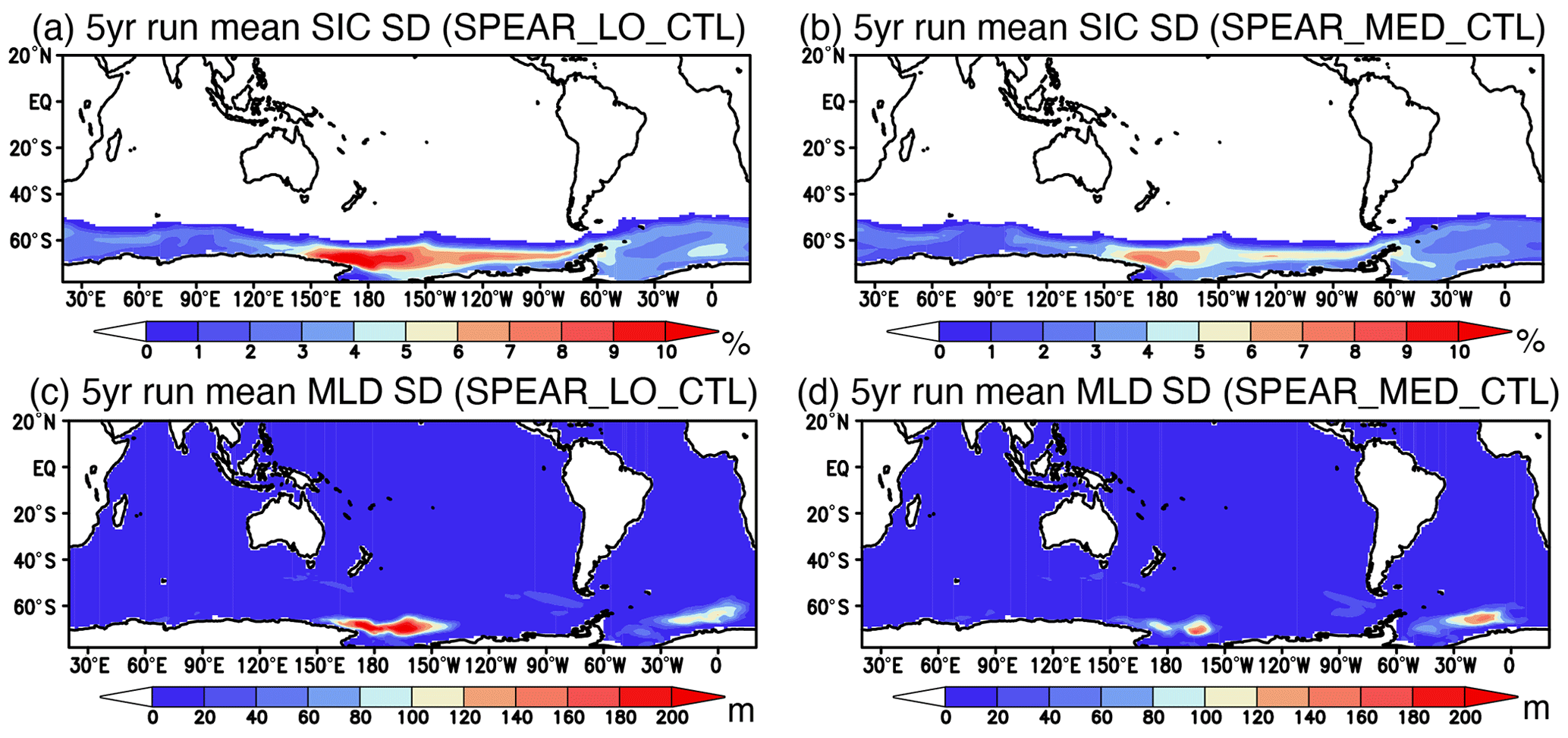
Figure 13(a) Standard deviation of 5-year running mean SIC (in %) anomalies from the SPEAR_LO_CTL with the preindustrial atmospheric radiative forcings. (b) Same as in (a), but for the SPEAR_MED_CTL. (c) Standard deviation of 5-year running mean mixed-layer-depth (MLD, in %) anomalies from the SPEAR_LO_CTL. (d) Same as in (c), but for the SPEAR_MED_CTL.
A recent study by Zhang et al. (2022a) has reported that the SPEAR_MED model (Delworth et al., 2020) with a higher atmospheric resolution tends to simulate a weaker deep convection variability in the Southern Ocean than the SPEAR_LO model. The standard deviation of 5-year running mean SIC anomalies from the 1000-year SPEAR_LO control simulation (SPEAR_LO_CTL) with the preindustrial atmospheric radiative forcing (Fig. 13a) is larger in the Pacific and Atlantic sectors than that from the SPEAR_MED control simulation (SPEAR_MED_CTL; Fig. 13b). This makes the SIC variability in the SPEAR_MED_CTL closer to the observed one (Fig. 1c) and appears to have links to smaller mixed-layer-depth variability in the SPEAR_MED_CTL (Fig. 13d) than in the SPEAR_LO_CTL (Fig. 13c). The weaker deep convection variability in the SPEAR_MED_CTL appears to contribute to the weaker mixed-layer variability and hence the weaker sea ice variability. Decadal reforecasts using the SPEAR_MED model may demonstrate more reasonable prediction skills of the Antarctic low-frequency sea ice variability than those using the SPEAR_LO model. Furthermore, the increase in the ocean resolution may help us better represent the mean state and variability of the Southern Ocean, which involves rich mesoscale eddies (Hallberg, 2013), thereby improving the decadal predictions, but this is beyond the scope of this study.
This study has further identified that the Southern Ocean deep convection gradually weakens after the 1990s and the surface wind variability starts to play a greater role in the Antarctic SIE increase after the 2000s. Weakening of the deep convection may be attributed to both an internal Southern Ocean multidecadal variability (Zhang et al., 2021) and a surface freshening owing to anthropogenic forcing (de Lavergne et al., 2014). On the other hand, the more frequent occurrence of a positive phase of the SAM tends to strengthen the westerly winds and induce northward transport of cold water and sea ice, leading to the Antarctic sea ice increase at a shorter timescale (e.g., J. Yang et al., 2021; Crosta et al., 2021). In addition, the southerly wind anomalies associated with the deepening of the Amundsen Sea Low assist in bringing more cold air from the Antarctica and enhancing sea ice formation in the Ross Sea (Turner et al., 2016; Meehl et al., 2016). Although the sources of decadal predictability remain unclear, the skillful prediction of the Antarctic SIE increase after the 2000s, which is not reproduced well in most of the CMIP5 models (Polvani and Smith, 2013; Yang et al., 2016), requires better representation of atmospheric circulation variability as well as ocean and sea ice variability in the Southern Ocean (Morioka et al., 2022).
The Antarctic SIE has experienced a slightly increasing trend over the past decades (Yuan et al., 2017; Parkinson, 2019). However, it has suddenly declined since 2016 and reached a record low in early 2022 (Simpkins, 2023). Several studies attributed the recent sea ice decrease to various factors including the upper Southern Ocean warming (Meehl et al., 2019; Zhang et al., 2022b), the anomalous warm air advection from the north (Turner et al., 2017; Wang et al., 2019), and the weakening of the midlatitude westerlies (Stuecker et al., 2017; Schlosser et al., 2018; Wang et al., 2019). However, it is unclear whether the sea ice decrease reflects an interannual or low-frequency variability or climate change (Eayrs et al., 2021), owing to a short observation record. We need to wait for this to be verified using more observational data when they become available in the future.
All codes to generate the figures can be provided upon the request to the corresponding author.
Monthly SIC data from HadISST1 and HadISST2 can be obtained from https://www.metoffice.gov.uk/hadobs/hadisst/data/download.html (Rayner et al., 2003) and https://www.metoffice.gov.uk/hadobs/hadisst2/data/download.html (Titchner and Rayner, 2014), respectively. Other monthly SIC data from the NOAA/NSIDC Climate Data Record website are also available here: https://doi.org/10.7265/efmz-2t65 (Meier et al., 2021). Monthly ocean temperature and salinity data can be downloaded from the EN4 website: https://www.metoffice.gov.uk/hadobs/en4/download.html (Good et al., 2013).
The supplement related to this article is available online at: https://doi.org/10.5194/tc-17-5219-2023-supplement.
YM performed data analysis and wrote the first draft of the manuscript, while LZ provided the reconstructed data and XY and FZ performed the model experiments. All authors commented on previous versions of the manuscript and approved the final manuscript.
The contact author has declared that none of the authors has any competing interests.
Publisher's note: Copernicus Publications remains neutral with regard to jurisdictional claims made in the text, published maps, institutional affiliations, or any other geographical representation in this paper. While Copernicus Publications makes every effort to include appropriate place names, the final responsibility lies with the authors.
We performed all of the SPEAR model experiments on the Gaea supercomputer at NOAA. We thank Rong Zhang, Mitch Bushuk, Yongfei Zhang, and William Gregory for providing constructive comments on the original manuscript. We are also grateful to two anonymous reviewers who provided valuable comments to improve the original manuscript. The present research is supported by Princeton University–NOAA GFDL Visiting Research Scientists program and base support of GFDL from NOAA Office of Oceanic and Atmospheric Research (OAR), JAMSTEC Overseas Research Visit Program, and JSPS KAKENHI grant numbers 19K14800 and 22K03727.
This research has been supported by Princeton University – NOAA GFDL Visiting Research Scientists program and base support of GFDL from NOAA Office of Oceanic and Atmospheric Research (OAR), JAMSTEC Overseas Research Visit Program, and JSPS KAKENHI (grant nos. 19K14800 and 22K03727).
This paper was edited by Xichen Li and reviewed by two anonymous referees.
Adcroft, A., Anderson, W., Balaji, V., Blanton, C., Bushuk, M., Dufour, C. O., Dunne, J. P., Griffies, S. M., Hallberg, R., Harrison, M. J., Held, I. M., Jansen, M. F., John, J. G., Krasting, J. P., Langenhorst, A. R., Legg, S., Liang, Z., McHugh, C., Radhakrishnan, A., Reichl, B. G., Rosati, T., Samuels, B. L., Shao, A., Stouffer, R., Winton, M., Wittenberg, A. T., Xiang, B., Zadeh, N., and Zhang, R.: The GFDL global ocean and sea ice model OM4.0: Model description and simulation features, J. Adv. Mod. Ear. Sys., 11, 3167–3211, https://doi.org/10.1029/2019MS001726, 2019.
Akitomo, K., Awaji, T., and Imasato, N: Open-ocean deep convection in the Weddell Sea: Two-dimensional numerical experiments with a nonhydrostatic model, Deep-Sea Res. Pt. I, 42, 53–73, https://doi.org/10.1016/0967-0637(94)00035-Q, 1995.
Blanchard-Wrigglesworth, E., Roach, L. A., Donohoe, A., and Ding, Q.: Impact of winds and Southern Ocean SSTs on Antarctic sea ice trends and variability, J. Climate, 34, 949–965, https://doi.org/10.1175/JCLI-D-20-0386.1, 2021.
Bushuk, M., Msadek, R., Winton, M., Vecchi, G., Yang, X., Rosati, A., and Gudgel, R.: Regional Arctic sea–ice prediction: potential versus operational seasonal forecast skill, Clim. Dynam., 52, 2721–2743, https://doi.org/10.1007/s00382-018-4288-y, 2019.
Bushuk, M., Winton, M., Haumann, F. A., Delworth, T., Lu, F., Zhang, Y., Jia, L., Zhang, L., Cooke, W., Harrison, M., Hurlin, B., Johnson, N. C., Kapnick, S. B., McHugh, C., Murakami, H., Rosati, A., Tseng, K., Wittenberg, A. T., Yang, X., and Zeng, F.: Seasonal Prediction and Predictability of Regional Antarctic Sea Ice, J. Climate, 34, 6207–6233, https://doi.org/10.1175/JCLI-D-20-0965.1, 2021.
Carsey, F. D.: Microwave observation of the Weddell Polynya, Mon. Weather Rev., 108, 2032–2044, https://doi.org/10.1175/1520-0493(1980)108<2032:MOOTWP>2.0.CO;2, 1980.
Cavalieri, D. J., Parkinson, C. L., and Vinnikov, K. Y.: 30-Year satellite record reveals contrasting Arctic and Antarctic decadal sea ice variability, Geophys. Res. Lett., 30, 1970, https://doi.org/10.1029/2003GL018031, 2003.
Cheon, W. G. and Gordon, A. L.: Open-ocean polynyas and deep convection in the Southern Ocean, Sci. Rep., 9, 1–9, https://doi.org/10.1038/s41598-019-43466-2, 2019.
Cheon, W. G., Park, Y. G., Toggweiler, J. R., and Lee, S. K.: The relationship of Weddell Polynya and open-ocean deep convection to the Southern Hemisphere westerlies, J. Phys. Oceanogr., 44, 694–713, https://doi.org/10.1175/JPO-D-13-0112.1, 2014.
Cheon, W. G., Lee, S. K., Gordon, A. L., Liu, Y., Cho, C. B., and Park, J. J.: Replicating the 1970s' Weddell polynya using a coupled ocean-sea ice model with reanalysis surface flux fields, Geophys. Res. Lett., 42, 5411–5418, https://doi.org/10.1002/2015GL064364, 2015.
Crosta, X., Etourneau, J., Orme, L. C., Dalaiden, Q., Campagne, P., Swingedouw, D., Goosse, H., Massé, G., Miettinen, A., McKay, R. M., Dunbar, R. B., Escutia, C., and Ikehara, M.: Multi-decadal trends in Antarctic sea-ice extent driven by ENSO–SAM over the last 2000 years, Nat. Geosci., 14, 156–160, https://doi.org/10.1038/s41561-021-00697-1, 2021.
de Lavergne, C., Palter, J. B., Galbraith, E. D., Bernardello, R., and Marinov, I.: Cessation of deep convection in the open Southern Ocean under anthropogenic climate change, Nat. Clim. Change, 4, 278–282, https://doi.org/10.1038/nclimate2132, 2014.
Delworth, T. L., Cooke, W. F., Adcroft, A., Bushuk, M., Chen, J.-H., Dunne, K. A., Ginoux, P., Gudgel, R., Hallberg, R. W., Harris, L., Harrison, M. J., Johnson, N., Kapnick, S. B., Lin, S.-J., Lu, F., Malyshev, S., Milly, P. C., Murakami, H., Naik, V., Pascale, S., Paynter, D., Rosati, A., Schwarzkopf, M. D., Shevliakova, E., Underwood, S., Wittenberg, A. T., Xiang, B., Yang, X., Zeng, F., Zhang, H., Zhang, L., and Zhao, M.: SPEAR: The next generation GFDL modeling system for seasonal to multidecadal prediction and projection, J. Adv. Mod. Ear. Sys., 12, e2019MS001895, https://doi.org/10.1029/2019MS001895, 2020.
Eade, R., Smith, D., Scaife, A., Wallace, E., Dunstone, N., Hermanson, L., and Robinson, N.: Do seasonal-to-decadal climate predictions underestimate the predictability of the real world?, Geophys. Res. Lett., 41, 5620–5628, https://doi.org/10.1002/2014GL061146, 2014.
Eayrs, C., Li, X., Raphael, M. N., and Holland, D. M.: Rapid decline in Antarctic sea ice in recent years hints at future change, Nat. Geosci., 14, 460–464, https://doi.org/10.1038/s41561-021-00768-3, 2021.
Eyring, V., Bony, S., Meehl, G. A., Senior, C. A., Stevens, B., Stouffer, R. J., and Taylor, K. E.: Overview of the Coupled Model Intercomparison Project Phase 6 (CMIP6) experimental design and organization, Geosci. Model Dev., 9, 1937–1958, https://doi.org/10.5194/gmd-9-1937-2016, 2016.
Ferreira, D., Marshall, J., Bitz, C. M., Solomon, S., and Plumb, A.: Antarctic Ocean and sea ice response to ozone depletion: A two-time-scale problem, J. Climate, 28, 1206–1226, https://doi.org/10.1175/JCLI-D-14-00313.1, 2015.
Fogt, R. L., Sleinkofer, A. M., Raphael, M. N., and Handcock, M. S.: A regime shift in seasonal total Antarctic sea ice extent in the twentieth century, Nat. Clim. Change, 12, 54–62, https://doi.org/10.1038/s41558-021-01254-9, 2022.
Francis, D., Eayrs, C., Cuesta, J., and Holland, D.: Polar cyclones at the origin of the reoccurrence of the Maud Rise Polynya in austral winter 2017, J. Geophys. Res.-Atmos., 124, 5251–5267, https://doi.org/10.1029/2019JD030618, 2019.
Francis, D., Mattingly, K. S., Temimi, M., Massom, R., and Heil, P.: On the crucial role of atmospheric rivers in the two major Weddell Polynya events in 1973 and 2017 in Antarctica, Sci. Adv., 6, eabc2695, https://doi.org/10.1126/sciadv.abc2695, 2020.
Gagné, M. È., Gillett, N. P., and Fyfe, J. C.: Observed and simulated changes in Antarctic sea ice extent over the past 50 years, Geophys. Res. Lett., 42, 90–95, https://doi.org/10.1002/2014GL062231, 2015.
Gong, D. and Wang, S.: Definition of Antarctic oscillation index, Geophys. Res. Lett., 26, 459–462, https://doi.org/10.1029/1999GL900003, 1999.
Good, S. A., Martin, M. J., and Rayner, N. A.: EN4: Quality controlled ocean temperature and salinity profiles and monthly objective analyses with uncertainty estimates, J. Geophys. Res.-Oceans, 118, 6704–6716, https://doi.org/10.1002/2013JC009067, 2013 (data available at: https://www.metoffice.gov.uk/hadobs/en4/download.html, last access: 21 February 2022).
Goosse, H. and Fichefet, T.: Open-ocean convection and polynya formation in a large-scale ice-ocean model, Tellus A, 53, 94–111, https://doi.org/10.1034/j.1600-0870.2001.01061.x, 2001.
Goosse, H. and Zunz, V.: Decadal trends in the Antarctic sea ice extent ultimately controlled by ice–ocean feedback, The Cryosphere, 8, 453–470, https://doi.org/10.5194/tc-8-453-2014, 2014.
Gordon, A. L.: Deep antarctic convection west of Maud Rise, J. Phys. Oceanogr., 8, 600–612, https://doi.org/10.1175/1520-0485(1978)008<0600:DACWOM>2.0.CO;2, 1978.
Gordon, A. L., Visbeck, M., and Comiso, J. C.: A possible link between the Weddell Polynya and the Southern Annular Mode, J. Climate, 20, 2558–2571, https://doi.org/10.1175/JCLI4046.1, 2007.
Guemas, V., Doblas-Reyes, F. J., Mogensen, K., Keeley, S., and Tang, Y.: Ensemble of sea ice initial conditions for interannual climate predictions, Clim. Dynam., 43, 2813–2829, https://doi.org/10.1007/s00382-014-2095-7, 2014.
Guemas, V., Chevallier, M., Déqué, M., Bellprat, O., and Doblas-Reyes, F.: Impact of sea ice initialization on sea ice and atmosphere prediction skill on seasonal timescales, Geophys. Res. Lett., 43, 3889–3896, https://doi.org/10.1002/2015GL066626, 2016.
Hallberg, R.: Using a resolution function to regulate parameterizations of oceanic mesoscale eddy effects, Ocean Model., 72, 92–103, https://doi.org/10.1016/j.ocemod.2013.08.007, 2013.
Hellmer, H. H., Kauker, F., and Timmermann, R.: Weddell Sea anomalies: Excitation, propagation, and possible consequences, Geophys. Res. Lett., 36, L12605, https://doi.org/10.1029/2009GL038407, 2009.
Henley, B. J., Gergis, J., Karoly, D. J., Power, S., Kennedy, J., and Folland, C. K.: A tripole index for the interdecadal Pacific oscillation, Clim. Dynam., 45, 3077–3090, https://doi.org/10.1007/s00382-015-2525-1, 2015.
Hobbs, W. R., Massom, R., Stammerjohn, S., Reid, P., Williams, G., and Meier, W.: A review of recent changes in Southern Ocean sea ice, their drivers and forcings, Global Planet. Change, 143, 228–250, https://doi.org/10.1016/j.gloplacha.2016.06.008, 2016.
Holland, P. R. and Kwok, R.: Wind-driven trends in Antarctic sea-ice drift, Nat. Geosci., 5, 872–875, https://doi.org/10.1038/ngeo1627, 2012.
Huang, B., Thorne, P. W., Banzon, V. F., Boyer, T., Chepurin, G., Lawrimore, J. H., Menne, M. J., Smith, T. M., Vose, R. S., and Zhang, H.: Extended Reconstructed Sea Surface Temperature, Version 5 (ERSSTv5): Upgrades, Validations, and Intercomparisons, J. Climate, 30, 8179–8205, https://doi.org/10.1175/JCLI-D-16-0836.1, 2017.
Killworth, P. D.: Deep convection in the world ocean, Rev. Geophys., 21, 1–26, https://doi.org/10.1029/RG021i001p00001, 1983.
Kobayashi, S., Ota, Y., Harada, Y., Ebita, A., Moriya, M., Onoda, H., Onogi, K., Kamahori, H., Kobayashi, C., Eendo, H., Miyaoka, K., and Takahashi, K.: The JRA-55 reanalysis: general specifications and basic characteristics, J. Meteorol. Soc. Japan. Ser. II, 93, 5–48, https://doi.org/10.2151/jmsj.2015-001, 2015.
Kriegler, E., Bauer, N., Popp, A., Humpenöder, F., Leimbach, M., Strefler, J., Baumstark, L., Bodirsky, B. L., Hilaire, J., Klein, D.,Mouratiadou, I., Weindl, I., Bertram, C., Dietrich, J.-P., Luderer, G., Pehl, M., Pietzcker, R., Piontek, F., Lotze-Campen, H., Biewald, A., Bonsch, M., Giannousakis, A., Kreidenweis, U., Müller, C., Rolinski, S., Schultes, A., Schwanitz, J., Stevanovic, M., Calvin, K., Emmerling, J., Fujimori, S., and Edenhofer, O.: Fossil-fueled development (SSP5): an energy and resource intensive scenario for the 21st century, Global Environ. Change, 42, 297–315, https://doi.org/10.1016/j.gloenvcha.2016.05.015, 2017.
Li, X., Holland, D. M., Gerber, E. P., and Yoo, C.: Impacts of the north and tropical Atlantic Ocean on the Antarctic Peninsula and sea ice, Nature, 505, 538–542, https://doi.org/10.1038/nature12945, 2014.
Marchi, S., Fichefet, T., Goosse, H., Zunz, V., Tietsche, S., Day, J. J., and Hawkins, E.: Reemergence of Antarctic sea ice predictability and its link to deep ocean mixing in global climate models, Clim. Dynam., 52, 2775–2797, https://doi.org/10.1007/s00382-018-4292-2, 2019.
Martinson, D. G., Killworth, P. D., and Gordon, A. L.: A convective model for the Weddell Polynya, J. Phys. Oceanogr., 11, 466–488, https://doi.org/10.1175/1520-0485(1981)011<0466:ACMFTW>2.0.CO;2, 1981.
Meehl, G. A., Arblaster, J. M., Bitz, C. M., Chung, C. T., and Teng, H. Antarctic sea-ice expansion between 2000 and 2014 driven by tropical Pacific decadal climate variability, Nat. Geosci., 9, 590–595, https://doi.org/10.1038/ngeo2751, 2016.
Meehl, G. A., Arblaster, J. M., Chung, C. T., Holland, M. M., DuVivier, A., Thompson, L., Yang, D., and Bitz, C. M.: Sustained ocean changes contributed to sudden Antarctic sea ice retreat in late 2016, Nat. Commun., 10, 1–9, https://doi.org/10.1038/s41467-018-07865-9, 2019.
Meier, W. N., Gallaher, D., and Campbell, G. G.: New estimates of Arctic and Antarctic sea ice extent during September 1964 from recovered Nimbus I satellite imagery, The Cryosphere, 7, 699–705, https://doi.org/10.5194/tc-7-699-2013, 2013.
Meier, W. N., Fetterer, F., Windnagel, A. K., and Stewart, J. S.: NOAA/NSIDC Climate Data Record of Passive Microwave Sea Ice Concentration, Version 4, Boulder, Colorado USA, National Snow and Ice Data Center [data set], https://doi.org/10.7265/efmz-2t65 (last access: 22 November 2022), 2021.
Morales Maqueda, M. A., Willmott, A. J., and Biggs, N. R. T.: Polynya dynamics: A review of observations and modeling, Rev. Geophys., 42, RG1004, https://doi.org/10.1029/2002RG000116, 2004.
Morioka, Y. and Behera, S. K.: Remote and local processes controlling decadal sea ice variability in the Weddell Sea, J. Geophys. Res.-Oceans, 126, e2020JC017036, https://doi.org/10.1029/2020JC017036, 2021.
Morioka, Y., Iovino, D., Masina, S., and Behera, S. K.: Role of sea-ice initialization in climate predictability over the Weddell Sea, Sci. Rep., 9, 1–11, https://doi.org/10.1038/s41598-019-39421-w, 2019.
Morioka, Y., Iovino, D., Cipollone, A., Masina, S., and Behera, S. K.: Summertime sea-ice prediction in the Weddell Sea improved by sea-ice thickness initialization, Sci. Rep., 11, 1–13, https://doi.org/10.1038/s41598-021-91042-4, 2021.
Morioka, Y., Iovino, D., Cipollone, A., Masina, S., and Behera, S. K.: Decadal Sea Ice Prediction in the West Antarctic Seas with Ocean and Sea Ice Initializations, Comm. Earth Env., 3, 1–10, https://doi.org/10.1038/s43247-022-00529-z, 2022.
Murphy, E. J., Clarke, A., Abram, N. J., and Turner, J.: Variability of sea-ice in the northern Weddell Sea during the 20th century, J. Geophys. Res.-Oceans, 119, 4549–4572, https://doi.org/10.1002/2013JC009511, 2014.
Orsi, A. H., Johnson, G. C., and Bullister, J. L.: Circulation, mixing, and production of Antarctic Bottom Water, Prog. Oceanogr., 43, 55–109, https://doi.org/10.1016/S0079-6611(99)00004-X, 1999.
Parkinson, C. L.: A 40-y record reveals gradual Antarctic sea ice increases followed by decreases at rates far exceeding the rates seen in the Arctic, P. Natl. Acad. Sci. USA, 116, 14414–14423, https://doi.org/10.1073/pnas.1906556116, 2019.
Polvani, L. M. and Smith, K. L.: Can natural variability explain observed Antarctic sea ice trends? New modeling evidence from CMIP5, Geophys. Res. Lett., 40, 3195–3199, https://doi.org/10.1002/grl.50578, 2013.
Power, S., Casey, T., Folland, C., Colman, A., and Mehta, V.: Inter-decadal modulation of the impact of ENSO on Australia, Clim. Dynam., 15, 319–324, https://doi.org/10.1007/s003820050284, 1999.
Rayner, N. A., Parker, D. E., Horton, E. B., Folland, C. K., Alexander, L. V., Rowell, D. P., Kent, E. C., and Kaplan, A.: Global analyses of sea surface temperature, sea ice, and night marine air temperature since the late nineteenth century, J. Geophys. Res., 108, 4407, https://doi.org/10.1029/2002JD002670, 2003 (data available at: https://www.metoffice.gov.uk/hadobs/hadisst/data/download.html, last access: 24 November 2022).
Riahi, K., Van Vuuren, D. P., Kriegler, E., Edmonds, J., O'neill, B. C., Fujimori, S., Bauer, N., Calvin, K., Dellink, R., Fricko, O., Lutz, W., Popp, A., Crespo Cuaresma, J., Kc, S., Leimbach, M., Jiang, L., Kram, T., Rao, S., Emmerling, J., Ebi, K., Hasegawa, T., Havlik, P., Humpenöder, F., Aleluia Da Silva, L., Smith, S., Stehfest, E., Bosetti, V., Eom, J., Gernaat, D., Masui, T., Rogel, J., Strefler, J., Drouet, L., Krey, V., Luderer, G., Harmsen, M., Takahashi, K., Baumstark, L., Doelman, J. C., Kainuma, M., Klimont, Z., Marangonii, G., Lotze-Campen, H., Obersteiner, M., Tabeau, A., and Tavoni, M.: The shared socioeconomic pathways and their energy, land use, and greenhouse gas emissions implications: an overview, Global Environ. Change, 42, 153–168, https://doi.org/10.1016/j.gloenvcha.2016.05.009, 2017.
Roach, L. A., Dörr, J., Holmes, C. R., Massonnet, F., Blockley, E. W., Notz, D., Rackow, T., Raphael, M. N., O'Farrell, S. P., Bailey, D. A., and Bitz, C. M.: Antarctic sea ice area in CMIP6, Geophys. Res. Lett., 47, e2019GL086729, https://doi.org/10.1029/2019GL086729, 2020.
Scaife, A. A. and Smith, D.: A signal-to-noise paradox in climate science, npj Clim. Atmos. Sci., 1, 28, https://doi.org/10.1038/s41612-018-0038-4, 2018.
Schlosser, E., Haumann, F. A., and Raphael, M. N.: Atmospheric influences on the anomalous 2016 Antarctic sea ice decay, The Cryosphere, 12, 1103–1119, https://doi.org/10.5194/tc-12-1103-2018, 2018.
Simpkins, G.: Record low Antarctic sea ice extent, Nat. Rev. Earth Environ., 4, 296, https://doi.org/10.1038/s43017-023-00433-w, 2023.
Stuecker, M. F., Bitz, C. M., and Armour, K. C.: Conditions leading to the unprecedented low Antarctic sea ice extent during the 2016 austral spring season, Geophys. Res. Lett., 44, 9008–9019, https://doi.org/10.1002/2017GL074691, 2017.
Sun, S. and Eisenman, I.: Observed Antarctic sea ice expansion reproduced in a climate model after correcting biases in sea ice drift velocity, Nat. Commun., 12, 1–6, https://doi.org/10.1038/s41467-021-21412-z, 2021.
Titchner, H. A. and Rayner, N. A.: The Met Office Hadley Centre sea ice and sea surface temperature data set, version 2: 1. Sea ice concentrations, J. Geophys. Res.-Atmos., 119, 2864–2889, https://doi.org/10.1002/2013JD020316, 2014 (data available at: https://www.metoffice.gov.uk/hadobs/hadisst2/data/download.html, last access: 24 November 2022).
Thompson, D. W. and Wallace, J. M.: Annular modes in the extratropical circulation. Part I: Month-to-month variability, J. Climate, 13, 1000–1016, https://doi.org/10.1175/1520-0442(2000)013<1000:AMITEC>2.0.CO;2, 2000.
Turner, J., Hosking, J. S., Marshall, G. J., Phillips, T., and Bracegirdle, T. J.: Antarctic sea ice increase consistent with intrinsic variability of the Amundsen Sea Low, Clim. Dynam., 46, 2391–2402, https://doi.org/10.1007/s00382-015-2708-9, 2016.
Turner, J., Phillips, T., Marshall, G. J., Hosking, J. S., Pope, J. O., Bracegirdle, T. J., and Deb, P.: Unprecedented springtime retreat of Antarctic sea ice in 2016, Geophys. Res. Lett., 44, 6868–6875, https://doi.org/10.1002/2017GL073656, 2017.
Turner, J., Guarino, M. V., Arnatt, J., Jena, B., Marshall, G. J., Phillips, T., Bajish, C. C., Clem, K., Wang, Z., Andersson, T., Murphy, E. J., and Cavanagh, R.: Recent decrease of summer sea ice in the Weddell Sea, Antarctica, Geophys. Res. Lett., 47, e2020GL087127, https://doi.org/10.1029/2020GL087127, 2020.
Venegas, S. A. and Drinkwater, M. R.: Sea ice, atmosphere and upper ocean variability in the Weddell Sea, Antarctica, J. Geophys. Res., 106, 16747–16765, https://doi.org/10.1029/2000JC000594, 2001.
Wang, G., Hendon, H. H., Arblaster, J. M., Lim, E. P., Abhik, S., and Rensch, P.: Compounding tropical and stratospheric forcing of the record low Antarctic sea-ice in 2016, Nat. Commun., 10, 1–9, https://doi.org/10.1038/s41467-018-07689-7, 2019.
Yang, C.-Y., Liu, J., Hu, Y., Horton, R. M., Chen, L., and Cheng, X.: Assessment of Arctic and Antarctic sea ice predictability in CMIP5 decadal hindcasts, The Cryosphere, 10, 2429–2452, https://doi.org/10.5194/tc-10-2429-2016, 2016.
Yang, J., Xiao, C., Liu, J., Li, S., and Qin, D.: Variability of Antarctic sea ice extent over the past 200 years, Sci. Bull., 66, 2394–2404, https://doi.org/10.1016/j.scib.2021.07.028, 2021.
Yang, X., Delworth, T. L., Zeng, F., Zhang, L., Cooke, W. F., Harrison, M. J., Rosati, A., Underwood, S., Compo, G. P., and McColl, C.: On the development of GFDL's decadal prediction system: Initialization approaches and retrospective forecast assessment, J. Adv. Mod. Earth Sys., 13, e2021MS002529, https://doi.org/10.1029/2021MS002529, 2021.
Yuan, N., Ding, M., Ludescher, and J., Bunde, A.: Increase of the Antarctic Sea Ice Extent is highly significant only in the Ross Sea, Sci. Rep., 7, 1–8, https://doi.org/10.1038/srep41096, 2017.
Yuan, X. and Martinson, D. G.: Antarctic sea ice extent variability and its global connectivity, J. Climate, 13, 1697–1717, https://doi.org/10.1175/1520-0442(2000)013<1697:ASIEVA>2.0.CO;2, 2000.
Zhang, L., Delworth, T. L., Cooke, W., and Yang, X.: Natural variability of Southern Ocean convection as a driver of observed climate trends, Nat. Clim. Change, 9, 59–65, https://doi.org/10.1038/s41558-018-0350-3, 2019.
Zhang, L., Delworth, T. L., Cooke, W., Goosse, H., Bushuk, M., Morioka, Y., and Yang, X.: The dependence of internal multidecadal variability in the Southern Ocean on the ocean background mean state, J. Climate, 34, 1061–1080, https://doi.org/10.1175/JCLI-D-20-0049.1, 2021.
Zhang, L., Delworth, T. L., Kapnick, S., He, J., Cooke, W., Wittenberg, A. T., Johnson, N. C., Rosati, A., Yang, X., Lu, F., Bushuk, M., McHugh, C., Murakami, H., Zeng, F., Jia, L., Tseng, K., and Morioka, Y.: Roles of Meridional Overturning in Subpolar Southern Ocean SST Trends: Insights from Ensemble Simulations, J. Climate, 35, 1577–1596, https://doi.org/10.1175/JCLI-D-21-0466.1, 2022a.
Zhang, L., Delworth, T. L., Yang, X., Zeng, F., Lu, F., Morioka, Y., and Bushuk, M.: The relative role of the subsurface Southern Ocean in driving negative Antarctic Sea ice extent anomalies in 2016–2021, Comm. Earth Environ., 3, 1–9, https://doi.org/10.1038/s43247-022-00624-1, 2022b.
Zhao, M., Golaz, J.-C., Held, I. M., Guo, H., Balaji, V., Benson, R., Chen, J.-H., Chen, X., Donner, L. J., Dunne, J. P., Dunne, K., Durachta, J., Fan, S.-M., Freidenreich, S. M., Garner, S. T., Ginoux, P., Harris, L. M., Horowitz, L. W., Krasting, J. P., Langenhorst, A. R., Liang, Z., Lin, P., Lin, S.-J., Malyshev, S. L., Mason, E., Milly, P. C. D., Ming, Y., Naik, V., Paulot, F., Paynter, D., Phillipps, P., Radhakrishnan, A., Ramaswamy, V., Robinson, T., Schwarzkopf, D., Seman, C. J., Shevliakova, E., Shen, Z., Shin, H., Silvers, L. G., Wilson, J. R., Winton, M., Wittenberg, A. T., Wyman, B., and Xiang, B.: The GFDL global atmosphere and land model AM4.0/LM4.0: 1. Simulation characteristics with prescribed SSTs, J. Adv. Mod. Earth Sys., 10, 691–734, https://doi.org/10.1002/2017MS001208, 2018a.
Zhao, M., Golaz, J.-C., Held, I. M., Guo, H., Balaji, V., Benson, R., Chen, J.-H., Chen, X., Donner, L. J., Dunne, J. P., Dunne, K., Durachta, J., Fan, S.-M., Freidenreich, S. M., Garner, S. T., Ginoux, P., Harris, L. M., Horowitz, L. W., Krasting, J. P., Langenhorst, A. R., Liang, Z., Lin, P., Lin, S.-J., Malyshev, S. L., Mason, E., Milly, P. C. D., Ming, Y., Naik, V., Paulot, F., Paynter, D., Phillipps, P., Radhakrishnan, A., Ramaswamy, V., Robinson, T., Schwarzkopf, D., Seman, C. J., Shevliakova, E., Shen, Z., Shin, H., Silvers, L. G., Wilson, J. R., Winton, M., Wittenberg, A. T., Wyman, B., and Xiang, B.: The GFDL global atmosphere and land model AM4.0/LM4.0: 2. Model description, sensitivity studies, and tuning strategies, J. Adv. Mod. Earth Sys., 10, 735–769, https://doi.org/10.1002/2017MS001209, 2018b.
Zunz, V., Goosse, H., and Dubinkina, S.: Impact of the initialisation on the predictability of the Southern Ocean sea ice at interannual to multi-decadal timescales, Clim. Dynam., 44, 2267–2286, https://doi.org/10.1007/s00382-014-2344-9, 2015.