the Creative Commons Attribution 4.0 License.
the Creative Commons Attribution 4.0 License.
 | 07 Feb 2023
Snow cover prediction in the Italian central Apennines using weather forecast and land surface numerical models
Edoardo Raparelli
Paolo Tuccella
Valentina Colaiuda
Frank S. Marzano
Italy is a territory characterized by complex topography with the Apennines mountain range crossing the entire peninsula and its highest peaks in central Italy. Using the latter as our area of interest and the snow seasons 2018/19, 2019/20 and 2020/21, the goal of this study is to investigate the ability of a simple single-layer and a more sophisticated multi-layer snow cover numerical model to reproduce the observed snow height, snow water equivalent and snow extent in the central Apennines, using for both models the same forecast weather data as meteorological forcing. We here consider two well-known ground surface and soil models: (i) Noah LSM, an Eulerian model which simulates the snowpack as a bulk single layer, and (ii) Alpine3D, a multi-layer Lagrangian model which simulates the snowpack stratification. We adopt the Weather Research and Forecasting (WRF) model to produce the meteorological data to drive both Noah LSM and Alpine3D at a regional scale with a spatial resolution of 3 km. While Noah LSM is already online-coupled with the WRF model, we develop here a dedicated offline coupling between WRF and Alpine3D. We validate the WRF simulations of surface meteorological variables in central Italy using a dense network of automatic weather stations, obtaining correlation coefficients higher than 0.68, except for wind speed, which suffered from the model underestimation of the real elevation. The performances of both WRF–Noah and WRF–Alpine3D are evaluated by comparing simulated and measured snow height, snow height variation and snow water equivalent, provided by a quality-controlled network of automatic and manual snow stations located in the central Apennines. We find that WRF–Alpine3D can predict better than WRF–Noah the snow height and the snow water equivalent, showing a correlation coefficient with the observations of 0.9 for the former and 0.7 for the latter. Both models show similar performances in reproducing the observed daily snow height variation; nevertheless WRF–Noah is slightly better at predicting large positive variations, while WRF–Alpine3D can slightly better simulate large negative variations. Finally we investigate the abilities of the models in simulating the snow cover area fraction, and we show that WRF–Noah and WRF–Alpine3D have almost equal skills, with both models overestimating it. The equal skills are also confirmed by Jaccard and the average symmetric surface distance indices.
- Article
(3972 KB) - Full-text XML
-
Supplement
(4674 KB) - BibTeX
- EndNote


Snow cover is a key element within global and local climate due to its high reflectivity of solar radiation and thermal insulation effects of land surfaces, inducing a non-linear feedback in the Earth energy balance (Hall, 2004). Snowpack melting is an essential water supply to sub-surface reservoirs, urban populations and agricultural activities which mainly rely on frozen water stored in the snowpack (Barnett et al., 2005). For mountainous touristic places the persistence of snow cover is the basis of their winter sport economy (Vanat, 2020). Nevertheless, the snowpack can be potentially dangerous when sliding down a slope, causing avalanches with possible major damage to local flora, fauna and even human settlements (Bebi et al., 2009).
The simulation of the seasonal snow cover is particularly challenging in mountainous regions because of the complex interaction between atmospheric flow and topography. Indeed the synoptic flow approaching the topography may lead to the formation of local phenomena, like orographic precipitation, that have a large influence on not only snow deposition patterns at the ridge scale but also smaller-scale phenomena, like preferential snow deposition and redistribution, which can cause large snow cover variations within a few meters (Mott et al., 2018). Thus the quality of a distributed simulation of the snow cover is closely related to the horizontal resolution and the quality of the atmospheric data used to force the snow cover model.
Recently the use of numerical weather prediction (NWP) models to drive snow cover models has been more and more investigated, thanks to improved computer performance that allows for increasing the spatial resolution and decreasing the computational time. Bellaire et al. (2011, 2013) and Bellaire and Jamieson (2013) simulated snow cover properties over British Columbia with the SNOWPACK model (Bartelt and Lehning, 2002; Lehning et al., 2002a, b), forced with atmospheric data provided by the NWP model GEM15 (Mailhot et al., 2006), suggesting the possibility of forcing snow cover models with simulated weather data where observations are not available and showing promising results on the possibility of predicting critical-layer formation. Still in western Canada, Schirmer and Jamieson (2015) showed that forcing SNOWPACK with the NWP model GEM-LAM (Erfani et al., 2005) at 2.5 km resolution provided better results than using the GEM15 model because of the former's higher resolution. Moreover, Horton et al. (2015) and Horton and Jamieson (2016) investigated the dependency of surface hoar formation on local meteorological and terrain conditions and the possibility of predicting them driving SNOWPACK with the GEM-LAM model. Vionnet et al. (2016) simulated the snowpack evolution over the French Alps driving the snow cover model Crocus (Vionnet et al., 2012) with the NWP model AROME (Seity et al., 2011), and Quéno et al. (2016) applied the same model chain to the French and Spanish Pyrenees. Bellaire et al. (2017) used SNOWPACK forced with the NWP model COSMO (Doms and Schättler, 2002) to forecast wet-snow avalanche activity in the Swiss Alps. Vionnet et al. (2017) forced Crocus with the NWP model Meso-NH (Lafore et al., 1997) at 50 m resolution, showing that for their case study in the French Alps, snow eolian transport is the main cause of snow height variability. Gerber et al. (2018) compared COSMO–WRF simulations (Skamarock et al., 2008) from 135 to 50 m resolution over the Swiss Alps to radar estimations, and they highlighted that in the presence of complex terrain, a good representation of the topography is essential to predict the observed snow precipitation and accumulation variability. Luijting et al. (2018) forced the Crocus model with AROME-MetCoOp-forecasted data (Müller et al., 2017) and a combination of AROME-MetCoOp and GridObs data (Lussana et al., 2018b, a) in southern Norway and showed that bias in GridObs data due to non-homogeneous distribution of automatic weather stations (AWSs) at different elevations affects the snowpack simulation, causing an early melt of the snow cover at high elevations. Vionnet et al. (2021) combined the High Resolution Deterministic Prediction System (HRDPS; Milbrandt et al., 2016) and the Canadian Hydrological Model (CHM; Marsh et al., 2020b, a), which allows for explicit snow redistribution modeling, and showed that the blowing-snow and gravitational-snow redistribution are necessary to reproduce the spatial variability in snowpack in alpine terrain. Lastly, Sharma et al. (2021) online-coupled WRF and SNOWPACK and introduced a new blowing-snow scheme. In this configuration, WRF drives SNOWPACK, which acts as a land surface model and gives feedback to WRF. This permits the simulation of a large number of snow layers, and thanks to the blowing-snow scheme even snow erosion and redistribution can be simulated, as the authors showed for case studies in Antarctica and the Swiss Alps.
Most of the cited works are focused on higher-latitude and higher-altitude mountain ranges, like the Canadian mountains, European Alps or Pyrenees, which have many peaks above 3000 m, or on cold regions like Antarctica. So far no study has focused on lower-latitude mountain ranges with peaks below 3000 m, such as the Italian Apennines. The latter are a series of mountains, bordered by narrow coastal lands and forming a great arc along the Italian Peninsula, from the Maritime Alps down to the Aegadian Islands in western Sicily. Their total length is about 1400 km, and their width goes from about 40 to 200 km. Their eastern slopes down to the Adriatic Sea are typically steeper and more verdant than the western ones. As a matter of fact, the Apennines play a significant role in the Italian climate, being a natural topographic barrier to both western Atlantic cyclonic fronts and eastern cold-air intrusions, causing intense snowfalls and hazardous avalanche activity (Chiambretti and Sofia, 2018) that may lead to fatal tragedies (Frigo et al., 2021). Its highest peak is Mount Corno Grande (2912 m) in the Gran Sasso chain in central Italy, belonging to the central Apennines in the Abruzzo region. The Gran Sasso also hosts the southernmost European paraglacier (glacial apparatus), named Calderone, a key sentinel of current climate change in the Mediterranean region. Due to their complex topography and relatively low altitudes, Apennines snow cover monitoring and forecasting are quite cumbersome and, to some extent, open further issues with respect to high-altitude mountainous regions.
The aim of this study is to investigate the ability of a simple single-layer and a more sophisticated multi-layer snow cover numerical model to reproduce the observed snow height, snow water equivalent and snow extent in the central Apennines, using for both models the same forecast weather data as meteorological forcing. To this purpose, we use two well-known snow and soil models: (i) Noah LSM, an Eulerian model which simulates the snowpack as a bulk single layer (Chen and Dudhia, 2001), and (ii) Alpine3D, a multi-layer Lagrangian model which simulates the snowpack stratification (Lehning et al., 2006). We adopt the Weather Research and Forecasting (WRF) model to produce the meteorological data to drive both Noah LSM and Alpine3D at a regional scale with a spatial resolution of 3 km.
While Noah LSM is already online-coupled with the WRF model, we develop here a dedicated offline coupling between WRF and Alpine3D for the first time, at least to the best of the authors' knowledge. The offline coupling of the two models gives the opportunity of running just Alpine3D in the case where WRF simulations have already been performed. This is particularly useful if different parametrizations have to be tested in Alpine3D only and not in WRF. Moreover, the offline coupling of WRF and Alpine3D may be easily used by the services that already use WRF operationally, by just installing Alpine3D and the interfacing library without the need to modify the already present WRF configuration. Nevertheless, it is important to note that the offline coupling of Alpine3D and WRF can be extended to other NWP models, just making small modifications to the interfacing library.
By means of the two numerical model chains WRF–Noah and WRF–Alpine3D, we simulate the snowpack evolution over the Italian central Apennines for three periods of interest: (i) from 1 December 2018 to 28 February 2019, (ii) from 1 March 2019 to 30 April 2020 and (iii) from 1 November 2020 to 30 April 2021. We compare the snow cover forecast results with in situ measurements of snow height and snow water equivalent and satellite-based radiometric observations of snow extent. In the following text we will refer to the three chosen periods of interest as snow seasons.
The present paper is structured as follows. In Sect. 2 we provide a brief description of the climate of the area of interest and a synoptic view of the three snow seasons. In Sect. 3 we describe the observation data set, the atmospheric model and the two land surface models, as well as the built numerical model chain. We then introduce the statistical indices used to evaluate the model skills. Finally, in Sect. 4 we compare and discuss observed and simulated data in terms of (i) atmospheric forcing, (ii) snow height, (iii) snow water equivalent and (iv) snow cover extent. Conclusions are drawn in the last section.
In this section we first introduce the climatology of the Italian central Apennines with a view of the synoptic characteristics for snow seasons 2018/19, 2019/20 and 2020/21. Meteorological charts of 500 hPa geopotential height, 850 hPa air temperature and surface precipitation anomalies are show in the Supplement.
2.1 Climatology of the Italian central Apennines
From a climatological point of view, inner central Italy is classified as marine climate, abbreviated as Cfb (C: temperate; f: no dry season; b: warm summer) according to the Köppen system (Köppen, 1931; Pinna, 1970; Belda et al., 2014). As a part of the Mediterranean region, the climate in this area of the Italian Peninsula is characterized by alternating rainy periods in winter months and dry periods during summer. In general, the temperature excursion, on a daily and annual basis, does not exceed 21 ∘C, due to the mitigating effect of both the Tyrrhenian and the Adriatic seas that surround a quite narrow strip of land, with an average width of ∼240 km in a W–E direction. Besides, due to its complex topography and elevations ranging from 0 to 2914 m a.s.l. (Corno Grande peak), in an extension of a few tens of kilometers, the area is also characterized by a high micro-climatic variability, from meso-Mediterranean to sub-continental temperate, in the inner part close to the highest peaks of the Apennines ridge (Lena et al., 2012).
According the statistics provided by Report no. 55 of the Italian Institute for Environmental Protection and Research (ISPRA, 2015), the annual average temperature in central Italy ranged from 5 ∘C (mountain areas) to 20 ∘C (coastal area) in the reference period 1981–2010. The minimum and maximum temperature values are between 3 and 11 ∘C and between 8 and 22 ∘C, respectively. Annual average accumulated precipitation is estimated to be between 600 and 1500 mm, with the yearly maxima mainly localized on the western slopes of the Apennine mountain range, exposed to the Tyrrhenian Sea. Minimum precipitation values occur over both the western and the eastern littoral areas. Summer coincides with the dry period, when accumulated precipitation ranges between 40 and 80 mm. In this context, it is worth mentioning that the average annual temperature and precipitation reported in the central Apennines area are 3.7 ∘C (−8.9 ∘C mean minimum temperature) and 1170 mm, respectively (Petriccione and Bricca, 2019).
In the central Apennines, the precipitation maxima are reached in autumn and spring and no drought period occurs during summer. As for the snow, mean solid precipitation depth (historical data from 1921 to 1960) on an annual basis ranged from 0–5 cm in the Tyrrhenian littoral area to a maximum value of 100–300 cm on the Apennines (Ministero dei Lavori Pubblici, 1973). Eastern slopes and the Adriatic side were found to have a greater average amount of snow, with climatological values of up to 20–50 cm in the coastal zone. Accordingly, the estimated number of chill days ranged from a minimum value of 0–1 on the western coast to 150–200 d in the inner part (Ministero dei Lavori Pubblici, 1973).
As observed by Libertino et al. (2018), Rossi (2020) and Alberton (2021), after the 1970s the fragmentation of the National Hydrographic Service into 20 different regional offices (1 per Italian region) led to the loss of homogeneity in meteorological data collection and statistics. While several studies are available in the Alps and northern Italy, central and southern Italy suffer from a low-density snow gauge network. Nevertheless, since the central Apennines are particularly prone to avalanche hazards, which have caused frequent casualties in the last few years, some authors have focused their attention on the occurrence of extreme snowfall events. Piacentini et al. (2020) have observed a decrease in snowfall, snow cover and snow persistence over the area in the last few decades, although a few extreme snowfall events have been recorded. High snow occurrence and accumulation variability in this part of Italy is also highlighted by Fazzini et al. (2021). Several authors have highlighted a decreasing trend in winter precipitation in central Italy in recent decades (Brunetti et al., 2000; Pavan et al., 2008; Longobardi and Villani, 2010; Romano and Preziosi, 2013; Appiotti et al., 2014; Scorzini and Leopardi, 2019). In the Gran Sasso d’Italia massif, the Interregional Association for coordination and documentation of snow and avalanche problems (AINEVA) has recorded a decreasing number of snow days at altitudes below 1300 m a.s.l. in the 30-year period of 1978–2007, even though events with intense snowfalls have been increasing in some specific areas (Romeo and Massimiliano, 2008).
2.2 Synoptic view
2.2.1 Snow season 2018/19
The snow season 2018/19 may be divided into three phases, from a synoptic point view. During December, the Euro-Mediterranean area was characterized by a strong positive 500 hPa geopotential height anomaly centered on the Iberian Peninsula, while a near-neutral or slightly negative geopotential anomaly affected eastern Europe. This resulted in a warm and dry pattern over the western Mediterranean Basin. By contrast, in January an oceanic anticyclonic system with above-normal geopotential heights determined a flux of Arctic cold air toward the Mediterranean through eastern Europe. This generated a generalized cold temperature anomaly over central and eastern Europe and the central Mediterranean Basin, with associated above-normal precipitation over the central and eastern Mediterranean Sea. Finally, February was dominated by a robust 500 hPa geopotential height anomaly extended to the whole continental Europe. As a result, the Euro-Mediterranean region was characterized by warm temperatures and dry conditions.
This pattern affected the precipitation in central Italy as follows. Between 10 and 20 December, the circulation over central Italy was affected by geopotential negative anomalies centered on eastern Europe. In the middle of December, cold-air advection from northern and northeastern Europe led to snowfall down to 700 m a.s.l., and the snowpack height measured at the observational sites ranged from 15 to 50 cm. During the second part of the month, the atmospheric conditions were influenced by the positive geopotential anomaly localized on the Iberian Peninsula. The associated mild weather caused a consistent lowering of snow height, especially at the middle- and low-altitude sampling sites.
The most important snowstorm of the season occurred between 2 and 4 January 2019, which resulted in an observed snow height in the range of 20–100 cm. Snowpack height did not show larger variations up to 22 January, due to the low temperatures and minor snowfall events. Between 23 and 24 January, thanks to cold-air advection from the North Atlantic, a mean of 40 cm of fresh snow was observed at our measurement sites.
An average lowering of 30 cm of the snow height was observed between 1 and 3 February, due to warm advection over Italy from north Africa. The rest of the month was characterized by a slow decay of snow height, due to general mild and dry atmospheric conditions.
2.2.2 Snow season 2019/20
The snow season 2019/20 was not favorable to the formation of a consistent snowpack. The western Mediterranean Basin was dominated by an extended positive geopotential height anomaly. Due to the mild and dry conditions resulting from this circulation pattern, only minor snowfall events occurred with the formation of a very thin snow cover at the highest elevation of our domain. This synoptic configuration was unblocked in March, which was characterized by a normal 500 hPa circulation with temperatures slightly under the average and precipitation above the climatology in central Italy. The most important snowstorm occurred at the end of March, when the snowpack reached a maximum height of 10–80 cm at our observational sites. The snowpack lowered immediately after the accumulation phase due to the relatively warm spring conditions and vanished before the middle of April.
2.2.3 Snow season 2020/21
The snow season 2020/21 may be divided in three phases. During December and January, Europe was subjected to strong negative 500 hPa geopotential height anomalies, resulting in wet conditions in our domain with near-average temperatures in December and cold conditions in January. By contrast, February was dominated by robust anticyclonic circulation which involved the Mediterranean, resulting in mild weather but a near-normal precipitation rate in our domain. Finally, March presented positive 500 hPa geopotential height anomalies over the British Isles, which determined a cold-air flux from Russia directed toward the Mediterranean but with below-normal precipitation in our domain of study.
The snowpack began to form at the end of November and remained of relatively thin heights up to the end of December. Starting from the end of 2020, a series of snowfall events were of interest in our domain until the end of January. In this period, the snow height ranged from 30 to 150 cm. In February, the snowpack height decreased due to the average warm conditions, although an important snowstorm occurred in the middle of the month. In March, a series of important snowfalls caused snow height up to 100–150 cm.
In this section we present the observational data, we describe the atmospheric and land surface models considered, and finally we define the performance evaluation methods.
3.1 Observational data set
The observational data set consists of in situ measurements of atmospheric and snow cover conditions, coming from AWSs and manual measurements, as well as of snow cover extent derived from satellite-based observations.
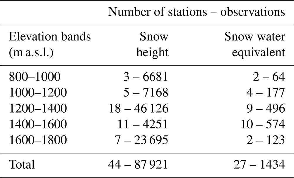
The in situ measurements come from a dense network of measurements sites which covers the entire study area. The measurement sites consist in 703 AWSs maintained by the Italian Civil Protection Department (Italian Civil Protection Department and CIMA Research Foundation, 2014) and 27 snow fields maintained by the Meteomont service (Rapisarda and Pranzo, 2021) (Fig. 1b). The variables provided by the AWSs are near-surface air temperature (∘C), relative humidity (%), wind speed (m s−1), incoming shortwave radiation (W m−2), precipitation (mm) and snow height (cm), while manual measurements provide snow height (cm) and the snowpack top layer density (kg m−3), which we used to derive the snowpack snow water equivalent (kg m−2) as described in the Supplement. Tables 1 and 2 show the number of measurement sites providing the above variables. The AWSs have an acquisition interval ranging between 15 min and 1 h, and they are sent to the Italian Civil Protection server every 15 min. We daily-averaged all observed variables, with the exception of precipitation, which we accumulated over 1 d, in order to set a common temporal framework. The snow height measurements are carried out with automatic ultra-sonic sensors, installed on 17 weather stations and located along the Italian central Apennines. Manual measurements in contrast are performed almost once per day every day for each Meteomont site; however the measurement frequency for snow seasons 2019/20 and 2020/21 was drastically reduced because of difficulties related to the COVID-19 pandemic.
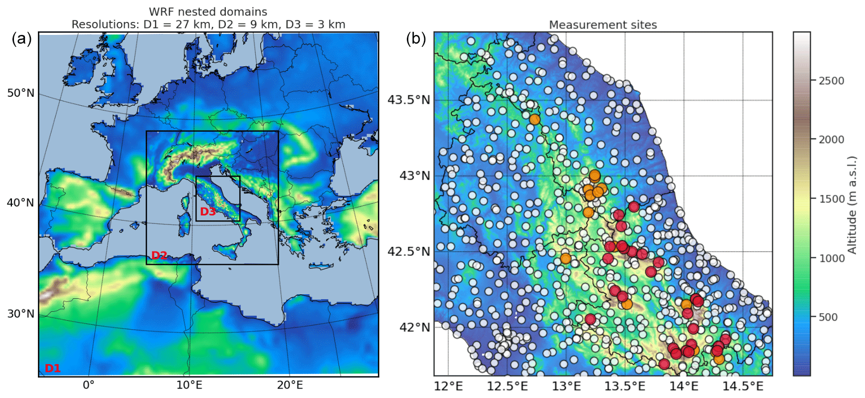
Figure 1(a) WRF nested domains D1, D2 and D3 with resolution 27, 9, and 3 km, respectively. (b) Atmospheric and snow measurement site locations in the D3 domain. The white circles represent automatic weather stations without a snow height sensor, while orange and red circles represent automatic weather stations with a snow height sensor and manual measurement sites, respectively.
Table 1Number of stations and observations for each of the analyzed variables at different elevation bands for the three snow seasons.
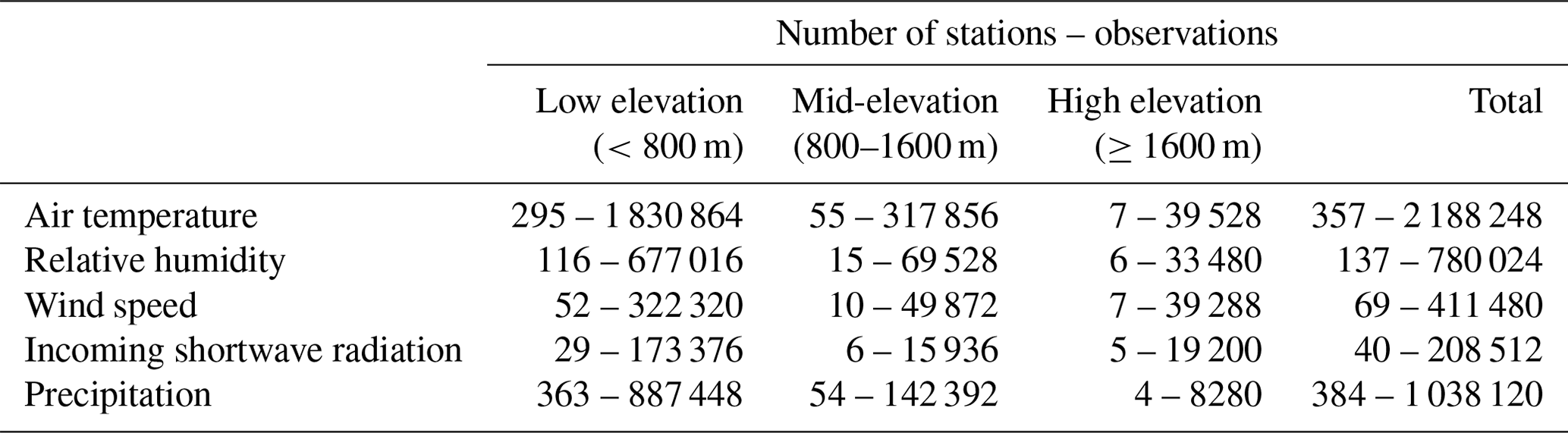
Table 2Number of snow stations and observations for different elevation bands for the three snow seasons.
Daily snow cover fraction is obtained from the MODIS Terra imaging sensor (product MOD10A1; Metsämäki et al., 2012). We used 275 maps of the snow cover fraction covering snow seasons 2018/19, 2019/20 and 2020/21. We first process MODIS maps in order to obtain cloud-free snow cover fraction maps as follows: the pixels classified as clouds are masked, and for each cloud pixel a linear interpolation between previous and consecutive images is carried out where the pixels are not cloud covered, in order to infer their fractional snow cover area. Then we regridded the cloud-free snow cover fraction maps on a regular grid of 3 km resolution.
In this section, we first introduce the weather forecast model, adopted and tuned to the study area of this work, as well as the two land surface models, specifically Noah LSM and Alpine3D. In the methodological paragraph we describe the error indices used to quantitatively evaluate the error statistics when comparing both WRF–Noah and WRF–Alpine3D with observational data.
3.2 Description of numerical models
The atmospheric and snow cover numerical models are here briefly described, highlighting the space–time setup and main physical parametrizations employed in this study.
3.2.1 Weather Research and Forecasting (WRF) model
The Weather Research and Forecasting (WRF) model is used in this work to describe the atmospheric evolution at the mesoscale. WRF is a regional non-hydrostatic meteorological model including several options for the parametrizations of atmospheric physical processes (Skamarock et al., 2008). As shown in Fig. 1a, the WRF atmospheric model is configured with three two-way nested domains. The largest domain has a 27 km spatial resolution, and the second domain has a 9 km spatial resolution, whereas the inner domain has a convection-permitting module at 3 km resolution. The vertical grid is constituted by 33 vertical levels extending from surface up to 50 hPa (about 20 km above the sea level) with the first level at 10 m from the surface.
The WRF main parametrizations include (i) the Yonsei University (YSU) scheme for the planetary boundary layer (Hong et al., 2006); (ii) the Rapid Radiative Transfer Model for general circulation model (RRTMG) for visible and infrared radiation (Iacono et al., 2008); (iii) the Thompson scheme for cloud microphysics (Thompson et al., 2008); and (iv) the Grell–Freitas scheme for cumulus convection (Grell and Freitas, 2014) with an exception for the cloud-resolving domain, where no cumulus parametrization is activated. The land cover classification used in WRF is based on the 20-class MODIS scheme.
The simulations cover three periods: (i) from 1 December 2018 to 28 February 2019, (ii) from 1 March 2019 to 30 April 2020 and (iii) from 1 November 2020 to 30 April 2021. For each season, the simulations start several days before the first snowfall occurred in all the measurement sites considered in order to spin up the surface and not introduce a bias into the evaluation of the performances of the land surface models, and to reduce the computational time.
Each season is simulated, concatenating several 60 h WRF simulations from which we discard the first 12 h as model spin-up. For each 60 h simulation the atmospheric conditions of the outer WRF domain are initialized with 6-hourly operational National Centers for Environmental Prediction (NCEP) analyses of 12:00 UTC at a resolution of 27 km, while for the nested domains, boundary conditions are derived from domain-1 and domain-2 simulations. This procedure is also used to initialize the land surface and soil properties for the first 60 h simulation of each snow season; in contrast the land surface and soil properties of the subsequent 60 h simulations of the season are obtained by the land surface and soil state at the end of the previous 60 h simulation. This procedure was chosen in order to avoid a discontinuous simulation of the snowpack in the study area. In order to improve the meteorological simulations, a spectral nudging toward NCEP analysis of wind, temperature and geopotential is applied in the outer domain above 850 hPa.
We have chosen this setup for WRF because it was revealed to be the best in simulating the main observed meteorological variables according to many preliminary sensitivity tests that we carried out.
3.2.2 Noah land surface model
Within the WRF model, land surface processes are simulated with Noah LSM (Chen and Dudhia, 2001). Noah LSM is a model that simulates skin temperature, snow height, snow water equivalent, snow density, soil moisture, soil temperature and surface energy balance. The snowpack is represented as a single layer of varying thickness; the soil is discretized in four layers of thickness 10, 30, 60 and 100 cm. Noah LSM is online-coupled with WRF, and it provides surface and latent heat fluxes as well as upward shortwave and longwave radiation to the parent model. The improvements in the Noah snowpack model introduced by Livneh et al. (2010) and Wang et al. (2010) were taken into account in our simulations.
As we discussed in the previous subsection, the initial conditions of Noah, for each snow season, are taken from the NCEP analysis, while for the rest of each season the land surface and soil state are simulated by the WRF–Noah chain. Starting the simulations of each snow season several days before the occurrence of the first snowfall at all the measurement sites, we obtain initial soil conditions representative of the initial soil state at those locations.
3.2.3 Alpine3D snow and soil model
Alpine3D is a three-dimensional snow cover, land surface and soil numerical model (Lehning et al., 2006). It includes the one-dimensional model SNOWPACK (Bartelt and Lehning, 2002; Lehning et al., 2002a, b) to simulate snow, land surface and soil properties; the SnowDrift module to simulate the wind transport of snow, the EBalance module to compute radiation fields taking into account topographic shading and reflection effects and a runoff module. SNOWPACK is the core of Alpine3D, it is developed using a Lagrangian scheme which permits to provide detailed description of snow stratigraphy, mass and energy balance, simulating up to 50 snow layers. In order to run an Alpine3D simulation, it is necessary to provide the initial state of snow and soil (if soil simulation is enabled), a digital elevation model, a land cover model and a meteorological input.
Alpine3D is not coupled with WRF so that it is necessary to interface the two models. First we had to re-project WRF output on a regular grid of 3 km resolution since Alpine3D does not support WRF curvilinear grid. In the Alpine3D configuration we used the digital elevation model and the land cover model also used for WRF simulations. We enabled in Alpine3D the soil simulation, creating four soil layers of 10, 30, 60 and 100 cm, respectively, and we initialized them using the soil condition extracted from Noah LSM at the first time-step of each snow season. For the remaining part of the simulation period, the land surface and soil state evolved according to Alpine3D. To drive Alpine3D, we use the air temperature, relative humidity, wind speed, incoming shortwave radiation, incoming longwave radiation, total precipitation, precipitation phase and ground surface temperature extracted and re-projected from WRF. WRF–Alpine3D hourly maps of snow height and snow water equivalent are then generated for each of the three snow seasons. A scheme of the described WRF–Alpine3D model chain is shown in Fig. 2.

Figure 2Flowchart of the model chain realized in this study. NCEP reanalyses are used to initialize the WRF model, which provides the atmospheric forcing data to drive WRF–Noah (online-coupled) and WRF–Alpine3D (offline-coupled) numerical models.
In our Alpine3D simulation setup, we turn off the SnowDrift and the EBalance modules: indeed, at the resolution of 3 km the wind transport of snow and the topographic shading and reflection effects have a negligible impact on the simulation results. Instead we enabled the canopy representation in the model, and after a sensitivity test (see Supplement), we opted for neutral atmospheric stability conditions for turbulent fluxes estimation as well as “Zwart” and “Lehning_1” parametrizations for new snow density and snow albedo, respectively (see Supplement for the parametrization descriptions). Since the soil simulation is active in Alpine3D, we can use the Richards water transport scheme instead of the more simple bucket scheme, even though it is more computationally demanding. Indeed in preliminary tests (not shown here), we observed that the Richards scheme increases the accuracy of Alpine3D in reproducing the observed snow height and snow water equivalent. Moreover, it is also known that the Richards scheme improves the performance of the model to estimate the meltwater runoff (Wever et al., 2014).
3.3 Evaluation methods
We here distinguish the error indices for atmospheric variable and snow height prediction from those used to estimate the discrepancy in the snow cover extension.
WRF skill in predicting the meteorological variables is evaluated comparing the output with in situ observations. The simulated air temperature, relative humidity, wind speed, incoming shortwave radiation and precipitation are bilinearly interpolated on the coordinates of the observed data. They are daily-averaged, with the exception of the precipitation rate, which is accumulated over 1 d. The simulated variables are statistically evaluated using mean bias error (MBE), mean absolute error (MAE) and the Pearson correlation coefficient (R) for three elevation bands (low elevation: <800 m, mid-elevation: 800–1600 m, high elevation: ≥1600 m).
The simulated snow height and snow water equivalent are bilinearly interpolated on the coordinates of the in situ observations and then re-sampled at a temporal resolution of 1 d. Starting from daily snow height, we derive the corresponding daily variations. In order to evaluate the model-based simulations of snow height, snow height variation and snow water equivalent, we use again MBE, MAE and R. For the snow height variation, the equitable threat score index (ETS) is also used (as proposed by Nurmi, 2003, and Schirmer and Jamieson, 2015) and quantify the skill of a forecast relative to chance, like snow height exceeding a certain threshold.
We are aware that the there is a strong scale mismatch between the point observations and kilometer resolution of the modeled data. And even if upscaling techniques have been proposed (Hou et al., 2022; Horton and Haegeli, 2022), we believe point measurements of snowpack properties are usually preferable, since they are directly taken on the field and their interpolation on a kilometer grid may even increase the degree of uncertainty in the evaluation of a model performances in reproducing the observations. Indeed, the interpolation of point snow measurements on a grid needs several assumptions about the wind transport of snow, vegetation interception, slope aspect and elevation which may also introduce uncertainty into the values used for validation. For these reasons, point data are widely used in the snow science community to validate model forecasts at kilometer resolution (Bellaire et al., 2011, 2013; Vionnet et al., 2012; Chen et al., 2014; Schirmer and Jamieson, 2015; Quéno et al., 2016; Luijting et al., 2018). Moreover, as suggested by Ikeda et al. (2010), Barlage et al. (2010) and Pavelsky et al. (2011), the scale mismatch between simulations at kilometer resolution and point observations can have a large impact if only one site is used for validation, but if a large number of validation sites are used, the mean model bias tends to be minimized, as the error at measurement sites tends to be randomly distributed. We also want to highlight that the measurement sites chosen in our paper are located in zones representative of large areas, in wide fields far from the canopy, and thus are particularly suitable to validate our simulations. However, in order to reduce the possible mismatch between the model resolution and the point observations, we divided the study domain into 200 m elevation bands, from 800 to 1800 m a.s.l. (Table 2), and for each elevation band we averaged the snow heights and snow water equivalents simulated and observed. We used the elevation-averaged values to calculate MBE, MAE and R evaluation indices.
The skill of WRF–Noah and WRF–Alpine3D model in reproducing the snow cover extent observed with MODIS is also evaluated. To this end, snow cover fraction maps are obtained for both WRF–Noah and WRF–Alpine3D from the following equation, equivalent to the empirical relation found by Koren et al. (1999):
where αs=2.6 is a distribution shape parameter, Ws is the simulated snow water equivalent, and Wmax is the snow-water-equivalent threshold above which the soil is 100 % covered with snow and varies locally according to MODIS land use classification (see Supplement). While Noah LSM already calculates the snow cover fraction according to Eq. (1), Alpine3D does not; thus we had to calculated it a posteriori using Eq. (1). By applying an arbitrary threshold of 51 %, we can build binary maps which indicate (i) snow absence if the snow cover fraction is below the threshold and (ii) snow presence if the snow cover fraction area is equal to or above the threshold. These binary maps are compared by using the Jaccard (J) index and the average symmetric surface distance (ASSD). The J index is equal to 1 if the binary maps perfectly overlap; alternatively it is equal to 0 if they do not overlap. The ASSD index ranges from 0 to ∞, and 0 means a perfect overlap of the boundaries of the binary maps. The application of ETS, J and ASSD to snowpack model validation is clearly described by Quéno et al. (2016).
From the snow cover binary maps of MODIS, WRF–Noah and WRF–Alpine3D, we finally calculate the respective snow cover area fraction, which is defined as the number of cells classified as snow divided by the total number of cells of the study domain. We compare the simulated snow cover area fractions with the one obtained from MODIS, and we evaluate them in terms of MBE, MAE and R. We also build and compare snow cover duration maps for MODIS, WRF–Noah and WRF–Alpine3D, counting the number of times that a cell was classified as covered with snow in the binary maps.
Both models, WRF–Noah and WRF–Alpine3D, are compared with observational data for the study area for snow seasons 2018/19, 2019/20, and 2020/21. The performance analysis is carried out in terms of the error indices, defined in the previous section, for both the atmospheric and the snow cover forecast.
4.1 Performance analysis of the atmospheric model
As a first validation, Fig. 3 shows the scatterplots of the comparison between simulated and measured daily air temperature, relative humidity, wind speed, incoming shortwave radiation and daily precipitation for the three snow seasons. The colors represent the observation density for each pixel; the brighter the color, the higher the density of observations for that pixel. The statistical scores, obtained from this intercomparison, are reported in Table 3 for the three elevation ranges defined in Sect. 3.3 and for all altitudes.
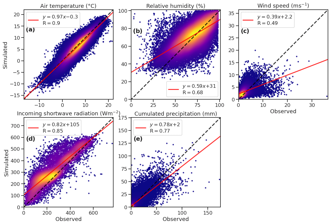
Figure 3Comparison of in situ observed data and WRF simulations of daily air temperature (a), relative humidity (b), wind speed (c), incoming shortwave radiation (d) and precipitation (e) for the three snow seasons. The density of observations for each pixel of the plot is represented with a color; the brighter the color, the higher the density of observations for that pixel.
Table 3WRF mean bias error (MBE), mean absolute error (MAE) and correlation coefficient (R) of air temperature, relative humidity, wind speed, incoming shortwave radiation and daily precipitation, for low elevation (<800 m), mid-elevation (800–1600 m) and high elevation (≥1600 m) bands for the three snow seasons.
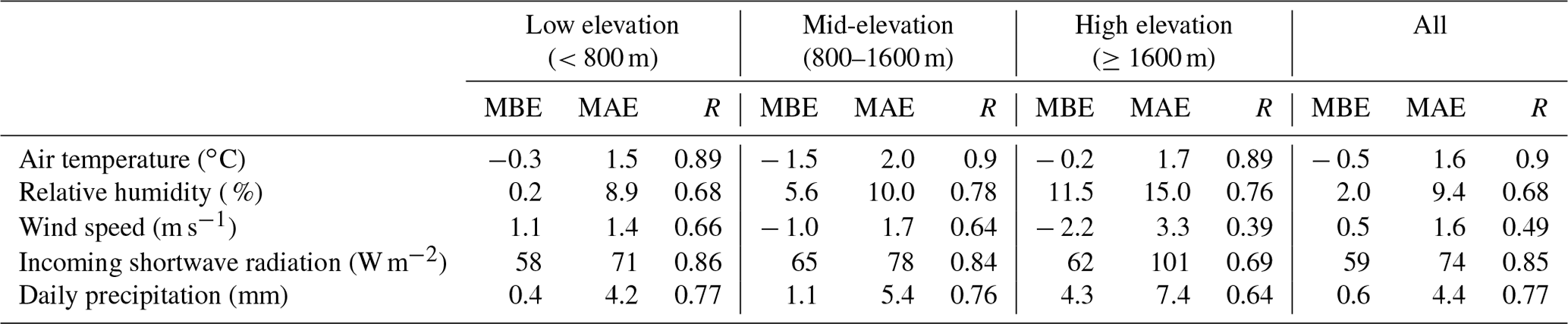
For the air temperature at all elevation ranges, WRF presents a correlation coefficient higher than 0.89, with an overall score of 0.9 (Fig. 3a). The WRF simulations exhibit a slightly negative MBE, especially for elevations between 800 and 1600 m, where they also show the highest MAE.
The relative humidity presents a correlation coefficient higher than 0.76 for mid-elevation and high-elevation bands but a lower one (0.68) for low elevations, with an overall score of 0.68 (Fig. 3b). The MBE and the MAE increase with the altitude.
From Fig. 3c we note that WRF in some cases drastically underestimates the wind speed. These points correspond to high-elevation measurement sites. Indeed at low elevations WRF shows a positive MBE, which decreases and becomes negative as the elevation increases. Clearly, the MAE shows an elevation dependence and increases from low to higher altitudes. Moreover, the correlation coefficient is minimum at high elevations and maximum at low elevations. The wind speed underestimation at high elevation is due to an underestimated elevation of the topography. Indeed the 3 km resolution of the model simulation smooths the highest peaks, causing a lower simulated wind speed at station locations (see Supplement for a comparison of model and real topography).
Figure 3d shows that WRF overestimates the incoming shortwave radiation. At high elevations, WRF has the highest MAE and the lowest correlation with the in situ observations. The general overestimation of incoming shortwave radiation is again partly due to the limited model horizontal resolution. Indeed the shading effect that influences the measured solar radiation may not be captured by the model, in which the topography is smoother and lower compared to reality.
Figure 3e highlights that WRF reproduces the daily precipitation with a correlation coefficient between 0.77 (for low elevations) and 0.64 (for high elevations). WRF shows the tendency to overestimate the precipitation as the altitude increases. Indeed, the bias is negligible below 800 m of altitude, but MBE reaches more than 4 mm at the high-altitude sites. This overestimation is likely due to the fact that rain gauges typically lose a precipitation fraction. When the precipitation is solid the underestimation is even larger because part of it is lost with sublimation, especially when the rain gauge is not heated.
In summary, for the WRF-simulated variables the overall correlation coefficient is above 0.68, except for the wind speed because as we already discussed, the strong negative bias at high elevations decreases the overall correlation to 0.49. On the other hand, it is well known that the wind speed field is particularly variable in complex orographic regions and a point-like in situ measurement cannot be representative of 3 km spatially averaged wind speed at the WRF model scales considered in this study.
4.2 Performance analysis of land surface models
4.2.1 Snow height
The time series intercomparison can be useful to show the temporal behavior of the two models with respect to in situ observations. The first row of Fig. 4 shows the mean snow height observed and simulated at all the measurement sites. Observations are indicated by a dashed gray line, while the numerical simulations are indicated by solid blue and red lines, corresponding to WRF–Noah and WRF–Alpine3D, respectively. The shaded areas correspond to the interval comprised between the minimum and maximum observed and simulated snow height.
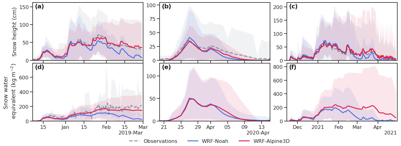
Figure 4Time series of observed and simulated snow height (a, b, c) and snow water equivalent (d, e, f) for the three snow seasons. Solid lines represent the mean of all available stations for each snow season considered: observations are indicated by a solid gray line, while simulations are indicated by solid blue and red lines, corresponding to WRF–Noah and WRF–Alpine3D, respectively. The shaded areas correspond to the maximum and minimum snow height and snow water equivalent observed or simulated. The low temporal frequency of the manual measurements for snow seasons 2019/20 and 2020/21 and the non-contemporaneity of the observations at different sites make the time series of the mean observed snow water equivalent noisy and uninformative; thus we decided to not show them in panels (e) and (f).
For snow season 2018/19 this comparison indicates that the mean snow height, simulated by the two models, is similar until mid-January, but during the last part of the snow season, WRF–Alpine3D better reproduces the observed snow height, also in terms of the settlement rate, while WRF–Noah underestimates the snow height, showing a faster settlement rate. In contrast for snow seasons 2019/20 and 2020/21, the differences in the mean snow heights simulated with WRF–Noah and WRF–Alpine3D are less evident, but especially in season 2020/21, it can be noticed that the snowpack shrinks faster in WRF–Noah simulations compared to the observation and WRF–Alpine3D simulations. This also has an impact on the maximum height simulated by the two models; indeed during the last part of each snow season, WRF–Noah largely underestimates the maximum snow height observed at the measurement sites, while WRF–Alpine3D has better skill in capturing the observed snow height variability between the measurement sites, simulating a maximum snow height closer to the observations. However, during April 2021 it can be noticed that WRF–Alpine3D overestimates the maximum snow height observed.
Another comparison of simulated and observed snow height for the three snow seasons is shown in the scatterplot of Fig. 5a, with blue indicating WRF–Noah and red WRF–Alpine3D. In order to reduce the possible mismatch between the model resolution and the point observations, observed and simulated values have been averaged for each of the elevation bands shown in Table 2. The plot shows that WRF–Alpine3D reproduces the snow height with more accuracy, especially when the observed snowpack is particularly thick. This results in a much higher correlation coefficient of WRF–Alpine3D compared to WRF–Noah (0.9 and 0.8, respectively) and in a negative bias of WRF–Noah in the snow height estimation (see Table 4 for all evaluation indices).
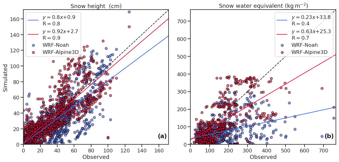
Figure 5Comparison of simulated and measured daily means of snow height (a) and snow water equivalent (b) averaged for each elevation band shown in Table 2 for the three snow seasons. Blue and red dots indicate WRF–Noah and WRF–Alpine3D, respectively. The blue and red lines represent the best linear fit of WRF–Noah and WRF–Alpine3D data.
Table 4WRF–Noah and WRF–Alpine3D mean bias error (MBE), mean absolute error (MAE) and correlation coefficient (R) for simulated snow height, daily snow height variation and snow water equivalent for the three snow seasons.

Snow height variation is an important indicator of the model skill in capturing the dynamical behavior of the snow cover. Thus, for the chosen AWSs, we compared simulated and observed snow height variations for the three snow seasons and we evaluated the model performances in terms of MBE, MAE and R. The results are shown in Table 4. In this case WRF–Alpine3D does not present better skills compared to WRF–Noah; indeed the models present almost the same correlation coefficient and MAE. A slight difference between the models can be seen in the MBE, which is slightly negative for WRF–Noah and positive for WRF–Alpine3D.
A more detailed view of the skill of WRF–Noah and WRF–Alpine3D in calculating the observed daily snow height variation comes from the analysis of Fig. 6a and b. Figure 6a shows the observed and modeled frequency distribution of daily snow height variation for the three snow seasons at the automatic validation sites used in this study. Gray columns represent the observed variations, and the blue and red columns represent the snow height variations simulated with WRF–Noah and WRF–Alpine3D, respectively. For the range of variations between [−20 cm, +30 cm), WRF–Noah and WRF–Alpine3D show similar performances, simulating a number of snow height variations for each class similar to the observations. Outside of this range, the behavior of the two models is clearly different. Below −20 cm, WRF–Alpine3D shows a better skill in reproducing the observed snow height variation, indeed variations in the interval [−30 cm, −20 cm) are missed from WRF–Noah. Instead for variations larger than 30 cm WRF–Noah seems to be more accurate in reproducing the observations compared to Alpine3D. The snow height variations observed in the range [40 cm, 50 cm) are not captured by both WRF–Noah and WRF–Alpine3D. Therefore, both models can well predict the central tendency of the distribution of the daily snow height variation, whereas they have more difficulties on the tails of the distribution. A further confirmation of this behavior comes from Fig. 6b, where the ETS index for different snow thresholds is reported. A look at Fig. 6b shows again that WRF–Noah and WRF–Alpine3D have similar scores between −1 cm and 10 cm thresholds, but they perform differently outside of this range. Indeed, compared to WRF–Alpine3D, WRF–Noah shows higher performances for snow height variations larger than 20 cm; however both models do not capture snow height variations larger than 40 cm. Instead, for variations smaller than −1 cm we can see that WRF–Alpine3D reaches scores larger than WRF–Noah. This suggests that WRF–Alpine3D has slightly better skills compared to WRF–Noah in predicting the observed snow settlement.
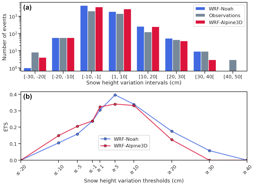
Figure 6(a) Observed and modeled frequency distribution of daily snow height variation for the three snow seasons obtained from the AWSs used in this study. The gray columns represent the observed variations, and the blue and red columns represent the snow height variations simulated with WRF–Noah and WRF–Alpine3D, respectively. (b) The ETS index for different snow thresholds with blue and red lines indicating WRF–Noah and WRF–Alpine3D scores, respectively.
4.2.2 Snow water equivalent
Snow water equivalent is a particularly interesting quantity because it represents the amount of mass stored in the snowpack. We derived snow-water-equivalent data combining manual measurements of snow height and snow density provided by the Meteomont service. The time series of the mean snow water equivalent, observed and simulated at all the manual sites, are shown in the second row of Fig. 4 for each snow season considered. Observations are indicated by a dashed gray line, while the numerical simulations are indicated by solid blue and red lines, corresponding to WRF–Noah and WRF–Alpine3D, respectively. The shaded areas correspond to the interval comprised between the minimum and maximum observed snow water equivalent.
As can be seen from Fig. 4d, during the snow season 2018/19, WRF–Noah and WRF–Alpine3D perform similarly during the accumulation phase, from December till mid-January, estimating a snow water equivalent really close to the observations. From mid-January till the end of the season, WRF–Alpine3D reproduces much better than WRF–Noah the snow-water-equivalent mean value and also its trend. Furthermore, especially during February, Alpine3D simulates maximum snow-water-equivalent values close to the observations, while WRF–Noah largely underestimates them. Unfortunately, during snow seasons 2019/20 and 2020/21, the manual measurements taken by the Meteomont service underwent a notable decrease because of the COVID-19 pandemic (Ciotti et al., 2020). The low temporal frequency and non-contemporaneity of the observations at different measurement sites make the time series of the mean observed snow water equivalent noisy and uninformative for the two snow seasons; thus we decided to not show it in Fig. 4e and f. Nevertheless, we can compare the two models, and we can observe that for snow season 2019/20 the mean snow water equivalents simulated by the two models almost overlap, but from 3 April WRF–Alpine3D simulates a larger maximum snowpack compared to WRF–Noah. In contrast during season 2020/21 the two models behave more similarly to season 2018/19; indeed it can be noticed that during the accumulation phase, from December till mid-January, the mean snow water equivalents simulated by the two models are very similar, but from mid-January till the end of the simulation, a much faster snowmelt in WRF–Noah compared to WRF–Alpine3D can be observed. The faster snowpack melt in WRF–Noah also has a large impact on the maximum snow water equivalent, which is much lower than in WRF–Alpine3D simulations, especially during March and April.
Looking again at the snow height time series shown in the first row of Fig. 4, we can notice that, in WRF–Alpine3D simulations, the snow height decrease does not correspond to a strong decrease in snow water equivalent (except for April 2021); instead in WRF–Noah a decrease in the snow height often corresponds to a large decrease in snow water equivalent. This means that the snowpack shrinking is mainly due to snow densification in WRF–Alpine3D and instead to snowmelt in WRF–Noah. The early melt of the snowpack observed in our WRF–Noah simulations during season 2018/19 at the chosen measurement sites is in line with the findings of Pavelsky et al. (2011), who for a case study on the Sierra Nevada, California, obtained an early snowmelt of 22–25 d in WRF–Noah simulations at 3 km resolution.
Another comparison of simulated and observed snow water equivalent for the three snow seasons is shown in the scatterplot of Fig. 5b, with blue indicating WRF–Noah and red WRF–Alpine3D. In order to reduce the possible mismatch between the model resolution and the point observations, observed and simulated values have been averaged for each of the elevation bands shown in Table 2. The plot shows that WRF–Alpine3D reproduces with more accuracy the snow water equivalent, especially for observed values between 150 and 350 kg m−2. This results in a much higher correlation coefficient of WRF–Alpine3D compared to WRF–Noah (0.7 and 0.4, respectively); however both models underestimate the snow water equivalent for observed values larger than 500 kg m−2 (see Table 4 for all evaluation indices).
4.2.3 Snow cover extent
The MODIS satellite snow product is an essential independent data set to evaluate the skill of WRF–Noah and WRF–Alpine3D in reproducing the observed snow cover area. As already described, the MODIS sensor provides the snow cover fraction (SCF) maps with 500 m resolution. Thanks to the applied cloud-removal algorithm, we have been able to also compare the snow cover extent for the days with a high cloud cover fraction.
As an example, Fig. 7a, b and c show the SCF maps obtained from MODIS, WRF–Noah and WRF–Alpine3D for 17 December 2018, which was one of the days with the largest observed snow cover area in snow season 2018/19. From the SCF maps, by applying a threshold of 51 %, we can derive the snow cover area (SCA), as shown in Fig. 7d, e and f. Forested areas, according to CORINE (European Union, Copernicus Land Monitoring Service 2018, European Environment Agency (EEA)) classification, are superimposed onto MODIS, WRF–Noah and WRF–Alpine3D data in order to qualitatively evaluate their impact on the snow cover area estimation. Snow cover within forested areas is a critical issue for snow mapping due to the forest signature on MODIS visible and near-infrared imagery, as highlighted by Gascoin et al. (2015). This results in an underestimation of the snow cover extent, especially during spring, when the snow is usually present below the forest but not on the trees, where it has already melted. Thus it cannot be excluded that WRF–Noah and WRF–Alpine3D overestimation of the snow cover area can be partially due to a MODIS underestimation of the snow cover area where forests are present.
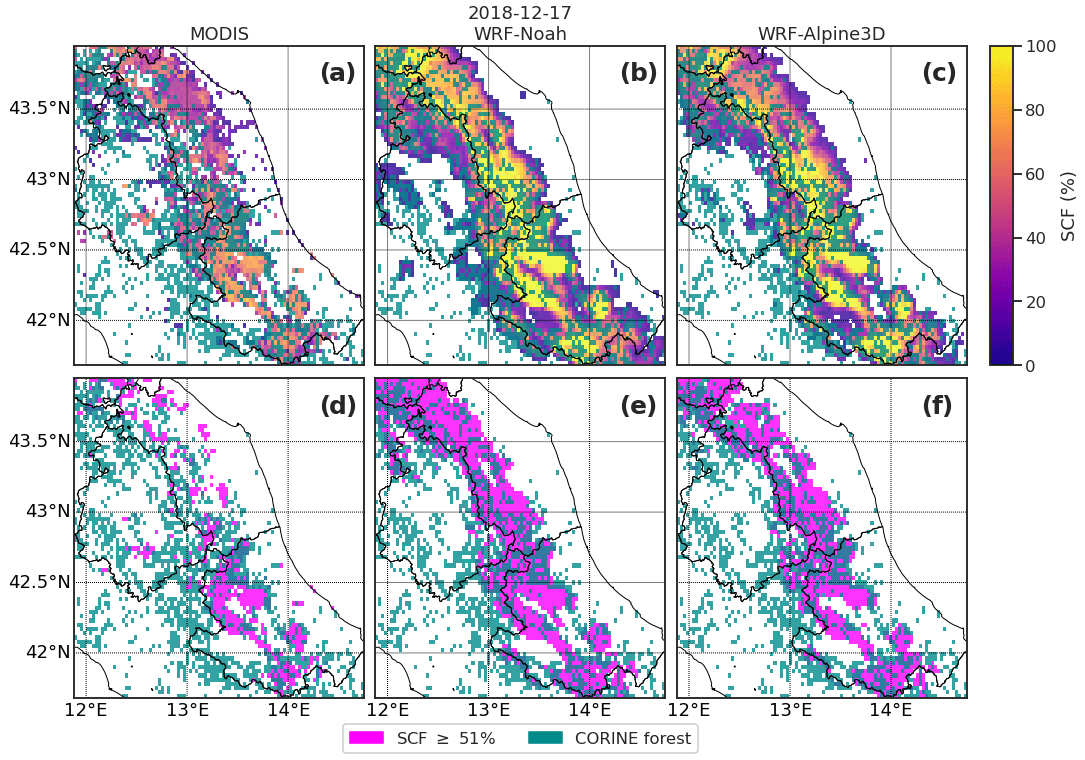
Figure 7(a, b, c) MODIS, WRF–Noah and WRF–Alpine3D snow cover fraction maps. (d, e, f) MODIS, WRF–Noah and WRF–Alpine3D snow cover area maps derived by applying a threshold of 51 % to the corresponding snow cover fraction maps. CORINE broadleaved-forest, coniferous-forest, and mixed-forest classes aggregated and reprojected from the original 100 m resolution to a 3 km resolution are also shown.
Duration of the snow cover is another important parameter, which has direct implications for many aspects, like local climate, water supply, and flora and fauna development. Figure 8 shows the observed and modeled snow cover duration maps, obtained counting the number of times that each cell is classified as covered with snow during the three snow seasons, within MODIS-, WRF–Noah- and WRF–Alpine3D-derived SCA maps. Figure 8 also shows the differences between the snow cover duration simulated with WRF–Noah and WRF–Alpine3D and the one obtained from MODIS. The difference between WRF–Alpine3D and WRF–Noah snow duration is also reported. These figures suggest that WRF–Noah and WRF–Alpine3D tend to simulate a longer snow cover duration over the entire central Apennines mountain range. The best agreement of the numerical models with the satellite-based observations is found at mountain tops and valley bottoms, as can be seen comparing Fig. 8 with the right panel of Fig. 1. By contrast, the largest differences emerge within middle-elevation zones, where both WRF–Noah and WRF–Alpine3D simulate a much longer snow cover duration. A closer inspection of Fig. 8d highlights noticeable differences between WRF–Noah and WRF–Alpine3D in the snow cover persistence. WRF–Noah simulates a more persistent snow cover when compared to WRF–Alpine3D over the northern part of the central Apennines, while WRF–Alpine3D predicts a longer snow cover duration in the southern part, especially in the Abruzzo region.

Figure 8(a, b, c) MODIS, WRF–Noah and WRF–Alpine3D snow cover duration maps derived from snow cover area maps for the three snow seasons. Panel (d) shows the differences in snow cover duration between WRF–Alpine3D and WRF–Noah, whereas panels (e) and (f) show the differences between MODIS and WRF–Noah and between MODIS and WRF–Alpine3D, respectively.
The snow cover area fraction (SCAF) can be computed over the chosen domain for each day of the study period, dividing the area classified as covered with snow by the total land area. The result of this calculation is reported in Fig. 9, and statistical indices obtained from this comparison are summarized in Table 5 for the three snow seasons. Both models reproduce the SCAF with a high correlation coefficient (0.89 and 0.88 for WRF–Noah and WRF–Alpine3D, respectively), but they overestimate the observed SCAF of 0.06. From these evaluations it emerges that the two models present almost identical performances in the estimation of the snow cover area fraction. However the SCAF does not take into account where the snow cover is present, and if observed and simulated snow patches are located in different places, the SCAF could be the same between observations and simulations.

Figure 9(a, b, c) Time series of snow cover area fraction derived from MODIS (gray line), WRF–Noah (blue line) and WRF–Alpine3D (red line) for the three snow seasons. (d) Comparison of simulated and observed snow cover area fraction for the three snow seasons, with blue and red dots indicating WRF–Noah and WRF–Alpine3D, respectively. The blue and red lines represent the best linear fit of WRF–Noah and WRF–Alpine3D data.
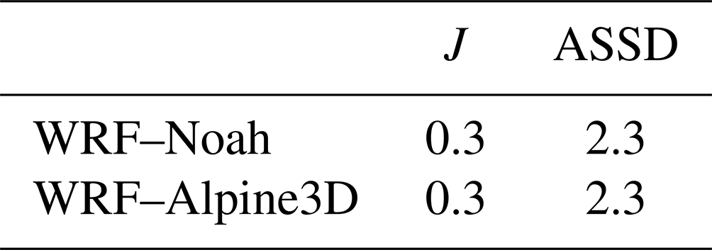
Thus, for each day of the three snow seasons, we have evaluated J and ASSD spatial indices, which also take into account where the snow patches are located, and we compared the SCA maps derived for WRF–Noah and WRF–Alpine3D with the ones derived from MODIS. J and ASSD time series are reported in Fig. 10, and their average values are summarized in Table 6. For J and ASSD WRF–Noah and Alpine3D exhibit identical mean values, confirming again that they have almost equal skills in reproducing the observed snow cover area.
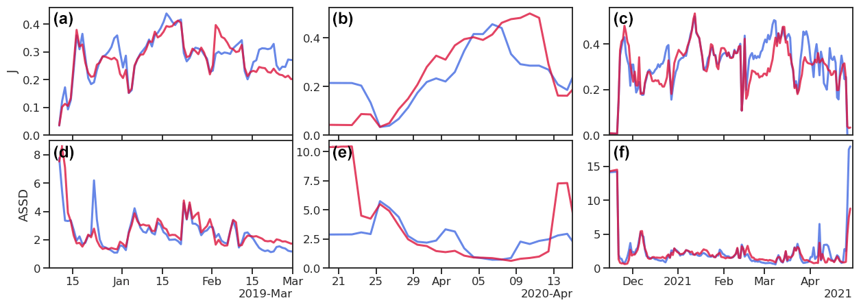
Figure 10Time series of the Jaccard index (a, b, c) and average symmetric surface distance index (d, e, f) computed for WRF–Noah (red line) and WRF–Alpine3D (blue line) for the three snow seasons.
Table 5WRF–Noah and WRF–Alpine3D mean bias error (MBE), mean absolute error (MAE) and correlation coefficient (R) for simulated snow cover area fractions for the three snow seasons.
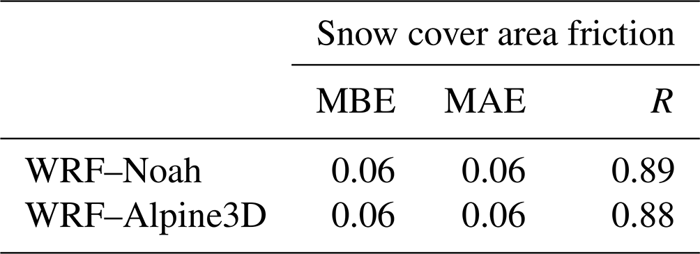
Table 6Mean values of the Jaccard index and average symmetric surface distance for WRF–Noah and WRF–Alpine3D for the three snow seasons.
We want to highlight that the SCF maps have been calculated in Noah with the inbuilt parametrization shown in Eq. (1) and in Alpine3D with the same parametrization but a posteriori. Moreover, we imposed the arbitrary threshold of 51 % to the SCF maps to derive the SCA maps (snow presence or absence), without performing a sensitivity test changing the threshold value. For these reasons, a change in the parametrization used for the calculation of the SCF maps or in the threshold applied to derive the SCA maps may lead to different model performances.
In this paper we have shown the different skills of Noah LSM and Alpine3D models in simulating the snow cover in the Italian central Apennines when forced with WRF atmospheric data during three snow seasons, going from December 2018 to April 2021. The study area is novel to snow cover studies, since most past works have focused on higher-latitude and higher-altitude mountain ranges or on cold regions. So far no study has focused on lower-latitude mountain ranges with peaks below 3000 m, like the central Apennines.
The performances of the WRF model in simulating air temperature, relative humidity, wind speed, incoming shortwave radiation and precipitation have first been evaluated, comparing them to observations derived from a dense network of automatic weather stations. The WRF model is capable of predicting the observed atmospheric variables with a correlation coefficient always higher than 0.68, except for the wind speed for which the model bias strongly increases with the altitude. We have also showed that during snow season 2018/19 WRF–Alpine3D is able to predict the observed snow height and snow water equivalent with higher accuracy compared to WRF–Noah, especially during February 2019. In general, during late-winter and spring periods, WRF–Alpine3D is able to reproduce the large snow height and snow water equivalent observed at some measurement sites, as opposed to WRF–Noah, which strongly underestimates it. We also observed that the snowpack shrinking is mainly due to snow densification in WRF–Alpine3D and instead to snowmelt in WRF–Noah. This is likely the reason why in WRF–Noah simulations the snowpack completely melts earlier than in the observations and WRF–Alpine3D simulations. In terms of daily snow height variation, WRF–Noah and WRF–Alpine3D present similar performances, with correlation coefficients slightly larger than 0.6, but still, the former shows a negative bias, while the latter shows a positive bias. The snow models are revealed to also have similar skills in predicting small daily snow height variations, but WRF–Noah performs slightly better at reproducing large positive daily variation, while WRF–Alpine3D has higher skills in predicting large negative variations.
Both models WRF–Noah and WRF–Alpine3D tend to overestimate the snow cover area fraction, provided by the MOD10A1 MODIS product. They present almost equal performances in the estimation of the snow cover area fraction. Also the comparison of the models through the Jaccard index (J) and the average symmetric surface distance (ASSD) confirmed that WRF–Noah and WRF–Alpine3D have almost the same skills in predicting shape, location and extension of the observed snow cover. However these findings strongly depend on the parametrization used to calculate the snow cover area fraction and on the threshold used to derive the snow cover area maps; thus using other parametrizations and thresholds may lead to different results.
Future work should be oriented to gather further in situ measurements of grain shape and grain size, necessary to quantify the abilities of WRF–Noah and WRF–Alpine3D to reproduce the observed snow microstructure. A way to improve WRF–Noah and WRF–Alpine3D performances would be to increase the horizontal spatial resolution of WRF simulations (e.g., from 3 km down to 1 km) in order to force the land surface models with more resolved atmospheric data. Increasing the WRF spatial resolution would also justify the activation in Alpine3D of the modules that take into account the eolian transport of snow, which redistributes the snow between adjacent cells of the domain according to the forecasted wind field, as well as the impact of the local topography on the energy balance through the effects of incoming shortwave radiation shading and longwave radiation increase. The WRF–Alpine3D simulation could also be improved by directly assimilating weather radar data in terms of the snowfall rate over the study domain in order to provide more realistic snow accumulation patterns. The approach for weather data assimilation, in terms of pointwise nudging or statistical variational techniques, is an interesting open issue.
The scripts developed within this work to interface and offline-couple WRF and Alpine3D numerical models are freely available at https://doi.org/10.5281/zenodo.7543614 (Raparelli, 2023).
The WRF–Noah and WRF–Alpine3D simulations are freely available at https://doi.org/10.5281/zenodo.7591394 (Raparelli and Tuccella, 2023). The automatic weather station data are provided upon request from the Italian Civil Protection Department and the hydrographic services of the Umbria, Marche, Abruzzo, Lazio and Molise regions. The manual snow measurements are freely provided from the Meteomont service. MODIS products are freely provided by the NASA National Snow and Ice Data Center. The CORINE Land Cover data set is freely provided by the Copernicus Land Monitoring Service.
The supplement related to this article is available online at: https://doi.org/10.5194/tc-17-519-2023-supplement.
ER carried out WRF–Alpine3D simulations; designed the work; and wrote the paper drafts leading the final version, including figures. PT carried out WRF simulations and contributed to designing the work as well as to writing and revising the paper. VC contributed to the climatological and meteorological description. FSM contributed to designing the work, as well as to writing and revising the paper, and managing the SMIVIA (Snow-mantle Modeling, Inversion and Validation using multi-frequency multi-mission InSAR in Central Apennines) project to co-fund the overall activity.
The contact author has declared that none of the authors has any competing interests.
Publisher’s note: Copernicus Publications remains neutral with regard to jurisdictional claims in published maps and institutional affiliations.
The authors are thankful to Mathias Bavay for support on the SNOWPACK and Alpine3D models; to Rossella Ferretti for the interesting discussions on numerical weather prediction modeling and for providing the computational resources to run Alpine3D simulations; to Massimo Pecci and Mauro Valt for sharing with us their experience in the interpretation of the snowpack properties.
This work was partially funded by the Italian Space Agency (Rome, Italy) within the SMIVIA project (contract no. 2021-9-U.0 CUP F85F21001230005).
This paper was edited by Emily Collier and reviewed by two anonymous referees.
Alberton, M.: Water Governance in Italy: From Fragmentation to Coherence Through Coordination Attempts, 355–368, Springer International Publishing, Cham, https://doi.org/10.1007/978-3-030-69075-5_15, 2021. a
Appiotti, F., Krželj, M., Russo, A., Ferretti, M., Bastianini, M., and Marincioni, F.: A multidisciplinary study on the effects of climate change in the northern Adriatic Sea and the Marche region (central Italy), Reg. Enviro. Change, 14, 2007–2024, https://doi.org/10.1007/s10113-013-0451-5, 2014. a
Barlage, M., Chen, F., Tewari, M., Ikeda, K., Gochis, D., Dudhia, J., Rasmussen, R., Livneh, B., Ek, M., and Mitchell, K.: Noah land surface model modifications to improve snowpack prediction in the Colorado Rocky Mountains, J. Geophys. Res.-Atmos., 115, D22, https://doi.org/10.1029/2009JD013470, 2010. a
Barnett, T. P., Adam, J. C., and Lettenmaier, D. P.: Potential impacts of a warming climate on water availability in snow-dominated regions, Nature, 438, 303–309, 2005. a
Bartelt, P. and Lehning, M.: A physical SNOWPACK model for the Swiss avalanche warning: Part I: numerical model, Cold Reg. Sci. Technol., 35, 123–145, https://doi.org/10.1016/S0165-232X(02)00074-5, 2002. a, b
Bebi, P., Kulakowski, D., and Rixen, C.: Snow avalanche disturbances in forest ecosystems – State of research and implications for management, Forest Ecol. Manage., 257, 1883–1892, https://doi.org/10.1016/j.foreco.2009.01.050, 2009. a
Belda, M., Holtanová, E., Halenka, T., and Kalvova, J.: Climate classification revisited: From Köppen to Trewartha, Clim. Res., 59, 1–13, https://doi.org/10.3354/cr01204, 2014. a
Bellaire, S. and Jamieson, B.: Forecasting the formation of critical snow layers using a coupled snow cover and weather model, Cold Reg. Sci. Technol., 94, 37–44, https://doi.org/10.1016/j.coldregions.2013.06.007, 2013. a
Bellaire, S., Jamieson, J. B., and Fierz, C.: Forcing the snow-cover model SNOWPACK with forecasted weather data, The Cryosphere, 5, 1115–1125, https://doi.org/10.5194/tc-5-1115-2011, 2011. a, b
Bellaire, S., Jamieson, J. B., and Fierz, C.: Corrigendum to ”Forcing the snow-cover model SNOWPACK with forecasted weather data” published in The Cryosphere, 5, 1115–1125, 2011, The Cryosphere, 7, 511–513, https://doi.org/10.5194/tc-7-511-2013, 2013. a, b
Bellaire, S., van Herwijnen, A., Mitterer, C., and Schweizer, J.: On forecasting wet-snow avalanche activity using simulated snow cover data, Cold Reg. Sci. Technol., 144, 28–38, https://doi.org/10.1016/j.coldregions.2017.09.013, 2017. a
Brunetti, M., Maugeri, M., and Nanni, T.: Variations of temperature and precipitation in Italy from 1866 to 1995, Theor. Appl. Climatol., 65, 165–174, https://doi.org/10.1007/s007040070041, 2000. a
Chen, F. and Dudhia, J.: Coupling an Advanced Land Surface–Hydrology Model with the Penn State–NCAR MM5 Modeling System. Part I: Model Implementation and Sensitivity, Mon. Weather Rev., 129, 569–585, https://doi.org/10.1175/1520-0493(2001)129<0569:CAALSH>2.0.CO;2, 2001. a, b
Chen, F., Barlage, M., Tewari, M., Rasmussen, R., Jin, J., Lettenmaier, D., Livneh, B., Lin, C., Miguez-Macho, G., Niu, G.-Y., Wen, L., and Yang, Z.-L.: Modeling seasonal snowpack evolution in the complex terrain and forested Colorado Headwaters region: A model intercomparison study, J. Geophys. Res.-Atmos., 119, 13795–13819, https://doi.org/10.1002/2014JD022167, 2014. a
Chiambretti, I. and Sofia, S.: Winter 2016–2017 snowfall and avalanche emergency management in Italy (Central Apennines) – A review, in: Proceedings of the International Snow Science Workshop, Innsbruck, Austria, 7–12, http://arc.lib.montana.edu/snow-science/item/2793 (last access: 5 February 2023), 2018. a
Ciotti, M., Ciccozzi, M., Terrinoni, A., Jiang, W.-C., Wang, C.-B., and Bernardini, S.: The COVID-19 pandemic, Crc. Cr. Rev. Cl. Lab. Sc., 57, 365–388, https://doi.org/10.1080/10408363.2020.1783198, 2020. a
Doms, G. and Schättler, U.: A description of the nonhydrostatic regional model LM, Part I: Dynamics and Numerics, Deutscher Wetterdienst, Offenbach, https://doi.org/10.5676/DWD_pub/nwv/cosmo-doc_6.00_I, 2002. a
Erfani, A., Mailhot, J., Gravel, S., Desgagné, M., King, P., Sills, D., McLennan, N., and Jacob, D.: The high resolution limited area version of the Global Environmental Multiscale model and its potential operational applications, 11th Conference on Mesoscale Processes, Session 1M, Mesoscale Model Development & Data Assimilation, Albuquerque, 2005. a
Fazzini, M., Cordeschi, M., Carabella, C., Paglia, G., Esposito, G., and Miccadei, E.: Snow Avalanche Assessment in Mass Movement-Prone Areas: Results from Climate Extremization in Relationship with Environmental Risk Reduction in the Prati di Tivo Area (Gran Sasso Massif, Central Italy), Land, 10, 1176, https://doi.org/10.3390/land10111176, 2021. a
Frigo, B., Bartelt, P., Chiaia, B., Chiambretti, I., and Maggioni, M.: A Reverse Dynamical Investigation of the Catastrophic Wood-Snow Avalanche of 18 January 2017 at Rigopiano, Gran Sasso National Park, Italy, Int. J. Disast. Risk. Sc., 12, 40–55, 2021. a
Gascoin, S., Hagolle, O., Huc, M., Jarlan, L., Dejoux, J.-F., Szczypta, C., Marti, R., and Sánchez, R.: A snow cover climatology for the Pyrenees from MODIS snow products, Hydrol. Earth Syst. Sci., 19, 2337–2351, https://doi.org/10.5194/hess-19-2337-2015, 2015. a
Gerber, F., Besic, N., Sharma, V., Mott, R., Daniels, M., Gabella, M., Berne, A., Germann, U., and Lehning, M.: Spatial variability in snow precipitation and accumulation in COSMO–WRF simulations and radar estimations over complex terrain, The Cryosphere, 12, 3137–3160, https://doi.org/10.5194/tc-12-3137-2018, 2018. a
Grell, G. A. and Freitas, S. R.: A scale and aerosol aware stochastic convective parameterization for weather and air quality modeling, Atmos. Chem. Phys., 14, 5233–5250, https://doi.org/10.5194/acp-14-5233-2014, 2014. a
Hall, A.: The Role of Surface Albedo Feedback in Climate, J. Climate, 17, 1550–1568, https://doi.org/10.1175/1520-0442(2004)017<1550:TROSAF>2.0.CO;2, 2004. a
Horton, S. and Haegeli, P.: Using snow depth observations to provide insight into the quality of snowpack simulations for regional-scale avalanche forecasting, The Cryosphere, 16, 3393–3411, https://doi.org/10.5194/tc-16-3393-2022, 2022. a
Horton, S. and Jamieson, B.: Modelling hazardous surface hoar layers across western Canada with a coupled weather and snow cover model, Cold Reg. Sci. Technol., 128, 22–31, https://doi.org/10.1016/j.coldregions.2016.05.002, 2016. a
Horton, S., Schirmer, M., and Jamieson, B.: Meteorological, elevation, and slope effects on surface hoar formation, The Cryosphere, 9, 1523–1533, https://doi.org/10.5194/tc-9-1523-2015, 2015. a
Hou, Y., Huang, X., and Zhao, L.: Point-to-Surface Upscaling Algorithms for Snow Depth Ground Observations, Remote Sens., 14, 4840, https://doi.org/10.3390/rs14194840, 2022. a
Iacono, M. J., Delamere, J. S., Mlawer, E. J., Shephard, M. W., Clough, S. A., and Collins, W. D.: Radiative forcing by long-lived greenhouse gases: Calculations with the AER radiative transfer models, J. Geophys. Res.-Atmos., 113, D13, https://doi.org/10.1029/2008JD009944, 2008. a
Ikeda, K., Rasmussen, R., Liu, C., Gochis, D., Yates, D., Chen, F., Tewari, M., Barlage, M., Dudhia, J., Miller, K., Arsenault, K., Grubišić, V., Thompson, G., and Guttman, E.: Simulation of seasonal snowfall over Colorado, Atmos. Res., 97, 462–477, https://doi.org/10.1016/j.atmosres.2010.04.010, 2010. a
ISPRA: Valori climatici normali di temperature e precipitazione in Italia, Stato dell’ambiente 55/2014, http://www.scia.isprambiente.it/wwwrootscia/Documentazione/rapporto_Valori_normali_def.pdf (last access: 2 February 2023), 2015. a
Italian Civil Protection Department and CIMA Research Foundation: The Dewetra Platform: A Multi-perspective Architecture for Risk Management during Emergencies, in: Information Systems for Crisis Response and Management in Mediterranean Countries, edited by: Hanachi, C., Bénaben, F., and Charoy, F., 165–177, Springer International Publishing, Cham, https://doi.org/10.1007/978-3-319-11818-5_15, 2014. a
Köppen, W.: Grundriss der klimakunde, Walter de Gruyter GmbH & Co KG, 1931. a
Koren, V., Schaake, J., Mitchell, K., Duan, Q.-Y., Chen, F., and Baker, J. M.: A parameterization of snowpack and frozen ground intended for NCEP weather and climate models, J. Geophys. Res.-Atmos., 104, 19569–19585, https://doi.org/10.1029/1999JD900232, 1999. a
Lafore, J. P., Stein, J., Asencio, N., Bougeault, P., Ducrocq, V., Duron, J., Fischer, C., Héreil, P., Mascart, P., Masson, V., Pinty, J. P., Redelsperger, J. L., Richard, E., and Vilà-Guerau de Arellano, J.: The Meso-NH Atmospheric Simulation System. Part I: adiabatic formulation and control simulations, Ann. Geophys., 16, 90–109, https://doi.org/10.1007/s00585-997-0090-6, 1998. a
Lehning, M., Bartelt, P., Brown, B., and Fierz, C.: A physical SNOWPACK model for the Swiss avalanche warning: Part III: meteorological forcing, thin layer formation and evaluation, Cold Reg. Sci. Technol., 35, 169–184, https://doi.org/10.1016/S0165-232X(02)00072-1, 2002a. a, b
Lehning, M., Bartelt, P., Brown, B., Fierz, C., and Satyawali, P.: A physical SNOWPACK model for the Swiss avalanche warning: Part II. Snow microstructure, Cold Reg. Sci. Technol., 35, 147–167, https://doi.org/10.1016/S0165-232X(02)00073-3, 2002b. a, b
Lehning, M., Völksch, I., Gustafsson, D., Nguyen, T. A., Stähli, M., and Zappa, M.: ALPINE3D: a detailed model of mountain surface processes and its application to snow hydrology, Hydrol. Process., 20, 2111–2128, https://doi.org/10.1002/hyp.6204, 2006. a, b
Lena, B., Antenucci, F., and Mariani, L.: Space and time evolution of the Abruzzo precipitation, Ital. J. Agrometeorol., 17, 5–20, 2012. a
Libertino, A., Ganora, D., and Claps, P.: Technical note: Space–time analysis of rainfall extremes in Italy: clues from a reconciled dataset, Hydrol. Earth Syst. Sci., 22, 2705–2715, https://doi.org/10.5194/hess-22-2705-2018, 2018. a
Livneh, B., Xia, Y., Mitchell, K. E., Ek, M. B., and Lettenmaier, D. P.: Noah LSM Snow Model Diagnostics and Enhancements, J. Hydrometeorol., 11, 721–738, https://doi.org/10.1175/2009JHM1174.1, 2010. a
Longobardi, A. and Villani, P.: Trend analysis of annual and seasonal rainfall time series in the Mediterranean area, Int. J. Climatol., 30, 1538–1546, https://doi.org/10.1002/joc.2001, 2010. a
Luijting, H., Vikhamar-Schuler, D., Aspelien, T., Bakketun, Å., and Homleid, M.: Forcing the SURFEX/Crocus snow model with combined hourly meteorological forecasts and gridded observations in southern Norway, The Cryosphere, 12, 2123–2145, https://doi.org/10.5194/tc-12-2123-2018, 2018. a, b
Lussana, C., Saloranta, T., Skaugen, T., Magnusson, J., Tveito, O. E., and Andersen, J.: seNorge2 daily precipitation, an observational gridded dataset over Norway from 1957 to the present day, Earth Syst. Sci. Data, 10, 235–249, https://doi.org/10.5194/essd-10-235-2018, 2018a. a
Lussana, C., Tveito, O. E., and Uboldi, F.: Three-dimensional spatial interpolation of 2 m temperature over Norway, Q. J. Roy. Meteor. Soc., 144, 344–364, https://doi.org/10.1002/qj.3208, 2018b. a
Mailhot, J., Bélair, S., Lefaivre, L., Bilodeau, B., Desgagné, M., Girard, C., Glazer, A., Leduc, A., Méthot, A., Patoine, A., Plante, A., Rahill, A., Robinson, T., Talbot, D., Tremblay, A., Vaillancourt, P., Zadra, A., and Qaddouri, A.: The 15‐km version of the Canadian regional forecast system, Atmos. Ocean, 44, 133–149, https://doi.org/10.3137/ao.440202, 2006. a
Marsh, C. B., Pomeroy, J. W., Spiteri, R. J., and Wheater, H. S.: A Finite Volume Blowing Snow Model for Use With Variable Resolution Meshes, Water Resour. Res., 56, e2019WR025307, https://doi.org/10.1029/2019WR025307, 2020a. a
Marsh, C. B., Pomeroy, J. W., and Wheater, H. S.: The Canadian Hydrological Model (CHM) v1.0: a multi-scale, multi-extent, variable-complexity hydrological model – design and overview, Geosci. Model Dev., 13, 225–247, https://doi.org/10.5194/gmd-13-225-2020, 2020b. a
Metsämäki, S., Mattila, O.-P., Pulliainen, J., Niemi, K., Luojus, K., and Böttcher, K.: An optical reflectance model-based method for fractional snow cover mapping applicable to continental scale, Remote Sens. Environ., 123, 508–521, https://doi.org/10.1016/j.rse.2012.04.010, 2012. a
Milbrandt, J. A., Bélair, S., Faucher, M., Vallée, M., Carrera, M. L., and Glazer, A.: The Pan-Canadian High Resolution (2.5 km) Deterministic Prediction System, Weather Forecast., 31, 1791–1816, https://doi.org/10.1175/WAF-D-16-0035.1, 2016. a
Ministero dei Lavori Pubblici: Carta della precipitazione nevosa media annua in Italia nel quarantennio 1921–1960: tavola rotonda della geografia della neve in Italia: Roma, 28–29 May 1973, https://books.google.it/books?id=QkCdoAEACAAJ (last access: 2 February 2023), 1973. a, b
Mott, R., Vionnet, V., and Grünewald, T.: The Seasonal Snow Cover Dynamics: Review on Wind-Driven Coupling Processes, Front. Earth Sci., 6, https://doi.org/10.3389/feart.2018.00197, 2018. a
Müller, M., Homleid, M., Ivarsson, K.-I., Koltzow, M. A. O., Lindskog, M., Midtbø, K. H., Andrae, U., Aspelien, T., Berggren, L., Bjorge, D., Dahlgren, P., Kristiansen, J., Randriamampianina, R., Ridal, M., and Vignes, O.: AROME-MetCoOp: A Nordic Convective-Scale Operational Weather Prediction Model, Weather Forecast., 32, 609–627, https://doi.org/10.1175/WAF-D-16-0099.1, 2017. a
Nurmi, P.: Recommendations on the verification of local weather forecasts, ECMWF Technical Memoranda, 430, 19 pp., https://doi.org/10.21957/y1z1thg5l, 2003. a
Pavan, V., Tomozeiu, R., Cacciamani, C., and Di Lorenzo, M.: Daily precipitation observations over Emilia-Romagna: mean values and extremes, Int. J. Climatol., 28, 2065–2079, https://doi.org/10.1002/joc.1694, 2008. a
Pavelsky, T. M., Kapnick, S., and Hall, A.: Accumulation and melt dynamics of snowpack from a multiresolution regional climate model in the central Sierra Nevada, California, J. Geophys. Res.-Atmos., 116, D16, https://doi.org/10.1029/2010JD015479, 2011. a, b
Petriccione, B. and Bricca, A.: Thirty years of ecological research at the Gran Sasso d’Italia LTER site: Climate change in action, Nature Conserv., 34, 9–39, https://doi.org/10.3897/natureconservation.34.30218, 2019. a
Piacentini, T., Calista, M., Crescenti, U., Miccadei, E., and Sciarra, N.: Seismically Induced Snow Avalanches: The Central Italy Case, Front. Earth Sci., 8, 507, https://doi.org/10.3389/feart.2020.599611, 2020. a
Pinna, M.: Contributo alla classificazione del clima d'Italia, Rivista Geografica Italiana, 77, 129–152, 1970. a
Quéno, L., Vionnet, V., Dombrowski-Etchevers, I., Lafaysse, M., Dumont, M., and Karbou, F.: Snowpack modelling in the Pyrenees driven by kilometric-resolution meteorological forecasts, The Cryosphere, 10, 1571–1589, https://doi.org/10.5194/tc-10-1571-2016, 2016. a, b, c
Raparelli, E: edrap/WRF2A3D: WRF-Alpine3D offline coupling script version 0.2.0-alpha, Zenodo [code], https://doi.org/10.5281/zenodo.7543614, 2023. a
Raparelli, E. and Tuccella, P.: WRF-Noah/Alpine3D simulations for 2018–2021 snow seasons in Italian Central Apennines, Zenodo [data set], https://doi.org/10.5281/zenodo.7591394, 2023. a
Rapisarda, A. and Pranzo, A. M. R.: Mapping the avalanche risk: from survey to cartographic production. The avalanche bulletin of the Meteomont Service of the Alpine Troops Command, Proc. Int. Cartogr. Assoc., 4, 92, https://doi.org/10.5194/ica-proc-4-92-2021, 2021. a
Romano, E. and Preziosi, E.: Precipitation pattern analysis in the Tiber River basin (central Italy) using standardized indices, Int. J. Climatol., 33, 1781–1792, https://doi.org/10.1002/joc.3549, 2013. a
Romeo, V. and Massimiliano, F.: La neve in Appennino. Prime analisi su 30 anni di dati meteonivologici, Neve e Valanghe, 63, https://issuu.com/aineva7/docs/nv63 (last access: 2 February 2023), 2008. a
Rossi, G.: Institutional Framework of Water Governance, 83–100, Springer International Publishing, Cham, https://doi.org/10.1007/978-3-030-36460-1_4, 2020. a
Schirmer, M. and Jamieson, B.: Verification of analysed and forecasted winter precipitation in complex terrain, The Cryosphere, 9, 587–601, https://doi.org/10.5194/tc-9-587-2015, 2015. a, b, c
Scorzini, A. R. and Leopardi, M.: Precipitation and temperature trends over central Italy (Abruzzo Region): 1951–2012, Theor. Appl. Climatol., 135, 959–977, https://doi.org/10.1007/978-3-030-36460-1_4, 2019. a
Seity, Y., Brousseau, P., Malardel, S., Hello, G., Bénard, P., Bouttier, F., Lac, C., and Masson, V.: The AROME-France Convective-Scale Operational Model, Mon. Weather Rev., 139, 976–991, https://doi.org/10.1175/2010MWR3425.1, 2011. a
Sharma, V., Gerber, F., and Lehning, M.: Introducing CRYOWRF v1.0: Multiscale atmospheric flow simulations with advanced snow cover modelling, Geosci. Model Dev. Discuss. [preprint], https://doi.org/10.5194/gmd-2021-231, in review, 2021. a
Skamarock, W. C., Klemp, J. B., Dudhia, J., Gill, D. O., Barker, D. M., Duda, M. G., Huang, X.-Y., Wang, W., and Powers, J. G.: A description of the advanced research WRF model version 3, National Center for Atmospheric Research: Boulder, CO, USA, p. 145, https://doi.org/10.5065/D68S4MVH, 2008. a, b
Thompson, G., Field, P. R., Rasmussen, R. M., and Hall, W. D.: Explicit Forecasts of Winter Precipitation Using an Improved Bulk Microphysics Scheme. Part II: Implementation of a New Snow Parameterization, Mon. Weather Rev., 136, 5095–5115, https://doi.org/10.1175/2008MWR2387.1, 2008. a
Vanat, L.: International Report on Snow & Mountain Tourism, https://www.vanat.ch/RM-world-report-2020.pdf (last access: 2 February 2023), 2020. a
Vionnet, V., Brun, E., Morin, S., Boone, A., Faroux, S., Le Moigne, P., Martin, E., and Willemet, J.-M.: The detailed snowpack scheme Crocus and its implementation in SURFEX v7.2, Geosci. Model Dev., 5, 773–791, https://doi.org/10.5194/gmd-5-773-2012, 2012. a, b
Vionnet, V., Dombrowski-Etchevers, I., Lafaysse, M., Quéno, L., Seity, Y., and Bazile, E.: Numerical Weather Forecasts at Kilometer Scale in the French Alps: Evaluation and Application for Snowpack Modeling, J. Hydrometeorol., 17, 2591–2614, https://doi.org/10.1175/JHM-D-15-0241.1, 2016. a
Vionnet, V., Martin, E., Masson, V., Lac, C., Naaim Bouvet, F., and Guyomarc'h, G.: High-Resolution Large Eddy Simulation of Snow Accumulation in Alpine Terrain, J. Geophys. Res.-Atmos., 122, 11005–11021, https://doi.org/10.1002/2017JD026947, 2017. a
Vionnet, V., Marsh, C. B., Menounos, B., Gascoin, S., Wayand, N. E., Shea, J., Mukherjee, K., and Pomeroy, J. W.: Multi-scale snowdrift-permitting modelling of mountain snowpack, The Cryosphere, 15, 743–769, https://doi.org/10.5194/tc-15-743-2021, 2021. a
Wang, Z., Zeng, X., and Decker, M.: Improving snow processes in the Noah land model, J. Geophys. Res.-Atmos., 115, D20, https://doi.org/10.1029/2009JD013761, 2010. a
Wever, N., Fierz, C., Mitterer, C., Hirashima, H., and Lehning, M.: Solving Richards Equation for snow improves snowpack meltwater runoff estimations in detailed multi-layer snowpack model, The Cryosphere, 8, 257–274, https://doi.org/10.5194/tc-8-257-2014, 2014. a