Mapping the extent of giant Antarctic icebergs with deep learning

Icebergs release cold, fresh meltwater and terrigenous nutrients as they drift and melt, influencing the local ocean properties, encouraging sea ice formation and biological production. To locate and quantify the fresh water flux from Antarctic icebergs, changes in their area and thickness have to be monitored along their trajectories. While the locations of large icebergs are operationally tracked by manual inspection, delineation of their extent is not. Here, we propose a U-net approach to automatically map the extent of giant icebergs in Sentinel-1 imagery. This greatly improves the efficiency compared to manual delineations, reducing the time for each outline from several minutes to less than 0.01 s. We evaluate the performance of our U-net and two state-of-the-art segmentation algorithms (Otsu and k-means) on 191 images. For icebergs larger than those covered by the training data, we find that U-net tends to miss parts. Otherwise, U-net is more robust in scenes with complex backgrounds – ignoring sea ice, smaller regions of nearby coast or other icebergs – and outperforms the other two techniques by achieving an F₁ score of 0.84 and an absolute median deviation in iceberg area of 4.1 %.

1 Introduction

Icebergs influence the environment along their trajectory through the release of cold, fresh water mixed with terrigenous nutrients (Duprat et al., 2016; Helly et al., 2011; Jenkins, 1999; Merino et al., 2016; Smith et al., 2007; Vernet et al., 2012). The more they melt, the higher the impact. However, this melting is not linear but depends on the surrounding ocean temperature, current speed and many other variables that are hard to model or observe (Bigg et al., 1997; Bouhier et al., 2018; England et al., 2020; Jansen et al., 2007; Silva et al., 2006). Calculating fresh water input from satellite observations is possible and can be partially automated. However, it requires manual delineations of the iceberg outlines to calculate the changes in the iceberg area and to collocate altimetry tracks with a map of initial iceberg thickness to estimate basal melting (Braakmann-Folgmann et al., 2021, 2022). Here, we present an automated approach using a U-net (Ronneberger et al., 2015) to segment giant Antarctic icebergs in Sentinel-1 images and hence to delineate their outline and area.

A number of methods including thresholding, edge-detection and clustering techniques have been proposed to automatically detect and segment icebergs in satellite radar imagery. Early work by Willis et al. (1996) was based on a thresholding technique and limited to certain iceberg sizes of a few hundred metres and certain wind conditions. Later, the constant false alarm rate (CFAR) thresholding technique was applied to detect icebergs in the Arctic (Frost et al., 2016; Gill, 2001; Power et al., 2001). Wesche and Dierking (2012) also used a threshold based on a K-distribution fitted to observed backscatter coefficients of icebergs, sea ice and open ocean followed by morphological operations. Mazur et al. (2017) developed an algorithm for iceberg detection in the Weddell Sea based on thresholds for, e.g. brightness, shape and size, at five scale levels applied to ENVISAT (Environmental Satellite) ASAR (Advanced Synthetic Aperture Radar) data. Apart from thresholding, edge-detection techniques have been applied. Williams et al. (1999) used a standard edge-detection technique followed by pixel bonding (Sephton et al., 1994) applied to European Remote-Sensing Satellite-1 (ERS-1) images during austral winter to detect and segment icebergs in East Antarctica. Silva and Bigg (2005) extended this to ENVISAT images and improved the algorithm by using another edge-detection technique. This was followed by a watershed segmentation and a classification step that takes area and shape into consideration but also requires manual interventions. A clustering technique was employed by Collares et al. (2018), who used the k-means algorithm (Macqueen, 1967) to segment icebergs, which were then manually tracked. Similarly, Koo et al. (2021) employed a built-in technique, similar to k-means, using Google Earth Engine to segment Sentinel-1 images and then applied an incidence-angle-dependent brightness threshold to find icebergs. They calculated the similarity of the distance to centroid histograms of all detected icebergs to the first instance, which was manually digitised, and then tracked one specific giant iceberg (B43). Finally, Barbat et al. (2019a) used a graph-based segmentation and ensemble forest committee classification algorithm with a range of hand-crafted (selected by a human operator) features.

Despite the quantity and variety of previous approaches, a range of limitations has hindered the operational application of an automated iceberg segmentation algorithm so far. One limitation is that previous studies have focused on smaller icebergs and performed worse for larger ones or were not even applicable to them (Mazur et al., 2017; Wesche and Dierking, 2012; Willis et al., 1996). Our work extends previous studies with the goal of delineating specific giant icebergs. Giant icebergs make up a very small part of the total iceberg population but hold the majority of the total ice volume (Tournadre et al., 2016), which makes them the most relevant for fresh water fluxes. Apart from iceberg size, there are many remaining challenges resulting from the variable appearance of icebergs and the surrounding ocean or sea ice in synthetic aperture radar (SAR) imagery (Ulaby and Long, 2014). The appearance of icebergs versus the surrounding ocean or sea ice depends on their surface roughness, the dielectric properties (e.g. moisture of the ice) and the satellite incidence angle (Ulaby and Long, 2014). Icebergs with dry, compact snow are usually bright targets in SAR images (Mazur et al., 2017; Wesche and Dierking, 2012; Young et al., 1998). While a calm ocean appears as a dark surface in SAR images, a wind-roughened sea appears brighter depending on the relative wind direction versus the satellite viewing angle (Young et al., 1998). Therefore, many studies report degrading accuracies in high-wind conditions (Frost et al., 2016; Mazur et al., 2017; Willis et al., 1996). Thin sea ice has a similar backscatter to a calm sea (Young et al., 1998), but rougher first-year ice already exhibits higher backscatter. Multiyear ice can reach backscatter values overlapping with the range of typical iceberg backscatter (Drinkwater, 1998). This explains why it is also mentioned that deformed sea ice or sea ice in general leads to false detections (Koo et al., 2021; Mazur et al., 2017; Silva and Bigg, 2005; Wesche and Dierking, 2012; Willis et al., 1996). Surface thawing can reduce the iceberg backscatter significantly (Young and Hyland, 1997). This means that those icebergs have the same backscatter as or lower backscatter than the surrounding ocean and sea ice, and appear as dark objects (Wesche and Dierking, 2012, see our Fig. 2, last column). Some of the existing techniques are therefore limited to austral winter images (Silva and Bigg, 2005; Williams et al., 1999), and dark icebergs remain a problem for all existing methods using SAR images. Furthermore, giant tabular icebergs can exhibit a gradient (Barbat et al., 2019a) due to variations in backscatter with the incidence angle (Wesche and Dierking, 2012) or appear heterogeneous due to crevasses (see Fig. 2, third and last column). This also complicates segmentation and differentiation from the surrounding ocean and sea ice. And finally, clusters of several icebergs and iceberg fragments too close to each other have been found to pose a problem (Barbat et al., 2019b; Frost et al., 2016; Koo et al., 2021; Williams et al., 1999). Our work aims to delineate icebergs in a variety of environmental conditions as accurately as possible using a deep learning technique.

Deep neural networks can encode the most meaningful features themselves and are able to learn more complex nonlinear relationships. Deep neural networks therefore outperform classic machine learning techniques in most tasks (LeCun et al., 2015; Schmidhuber, 2015). U-net is a neural network that was originally developed for biomedical image segmentation (Ronneberger et al., 2015). It has since been applied to many other domains including satellite imagery and polar science (Andersson et al., 2021; Baumhoer et al., 2019; Dirscherl et al., 2021; Kucik and Stokholm, 2023; Mohajerani et al., 2019, 2021; Poliyapram et al., 2019; Singh et al., 2020; Stokholm et al., 2022; Surawy-Stepney et al., 2023; Zhang et al., 2019). U-net works well with a few training examples, trains quickly and still achieves very good results (Ronneberger et al., 2015). A comparison between three network architectures (Deeplab, DenseNet and U-net) for river ice segmentation found that U-net provided the best balance between quantitative performance and good generalisation (Singh et al., 2020). Baumhoer et al. (2019) used a U-net architecture to automatically delineate ice shelf fronts in Sentinel-1 images with good success (108 m average deviation). The calving front to ocean boundary involves similar conditions and challenges to an iceberg to ocean boundary. Because of the many successful studies using U-net, including one with similar challenges (Baumhoer et al., 2019), we decided to also employ a U-net.

2 Data

This section describes the Sentinel-1 input data and generation of the manually derived outlines for training, validation and testing. The goal is to derive the outlines of Antarctic icebergs, which are large enough to receive a name and to be operationally tracked. Therefore, we generate a binary segmentation map in which the biggest iceberg present in the image is selected and everything else – including smaller icebergs, iceberg fragments and adjacent land ice – is considered as background. This approach differs from most previous work. In most previous work the goal was to find all icebergs. In contrast, our work is targeted to monitor changes in area of these large icebergs but also to track how the icebergs rotate and use their outline to automatically collocate altimetry overpasses (Braakmann-Folgmann et al., 2022).

2.1 Sentinel-1 input imagery

The Sentinel-1 satellites measure the backscatter of the surface beneath them using SAR. In contrast to optical imagery, SAR provides data throughout the polar night and independent of cloud cover (Ulaby and Long, 2014). The Sentinel satellites are an operational satellite system with free data availability (Torres et al., 2012). Sentinel-1a (2014–present) and Sentinel-1b (2016–2022) had a combined repeat cycle of 6 d (Torres et al., 2012), but the polar regions are sampled more frequently. We use the Level-1 Ground Range Detected (GRD) data at medium resolution. Depending on the geographic location around Antarctica, data are collected in either interferometric wide (IW) or extra wide (EW) swath mode. IW is a 250 km wide swath with 5 × 20 m native spatial resolution and EW is a 400 km wide swath with 20 × 40 m native resolution. We use both modes depending on availability. While HH-polarised (horizontal transmit and horizontal receive) data are available across the Southern Ocean, HV (horizontal transmit and vertical receive) data are only available in some parts. As icebergs drift across these acquisition masks and HH has been found to give the best results for iceberg detection (Sandven et al., 2007), we use the HH-polarised data only. Should both modes become available across the Southern Ocean in the future, their collective use might be advantageous. Icebergs and their surroundings cause different changes in polarisation, which could be exploited using e.g. the HH $/$ HV ratio.

We preprocess and crop the Sentinel-1 images before applying the segmentation techniques. Firstly, we apply the precise orbit file, remove thermal noise and apply a radiometric calibration. We also multilook the data with a factor of 6 to reduce speckle and image size, yielding a square pixel spacing of 240 m. Then we apply a terrain correction using the GETASSE30 (global earth topography and sea surface elevation at 30 arcsec resolution) digital elevation model and project the output on a polar stereographic map with a true latitude of 71^∘ S. These preprocessing steps are conducted on the Sentinel Application Platform (SNAP). All icebergs that are longer than 18.5 km (10 nautical miles) or that encompass an area of at least 68.6 km² (20 square nautical miles) are named and tracked operationally every week by the U.S. National Ice Center (NIC). These are referred to as “giant” icebergs (Silva et al., 2006). In addition, these and smaller icebergs (longer than 6 km) are tracked by Brigham Young University (Budge and Long, 2018), which releases daily positions every few years. Therefore, we have a good estimate of where each of these giant icebergs should be. We can firstly download targeted Sentinel-1 images containing these icebergs and secondly crop the images around the estimated central position to a size of 256 × 256 pixels. Hence, every input image contains a giant target iceberg. Some images contain several icebergs and in this case we are only interested in the largest one. To ensure that the largest icebergs fit within the image, we rescale images of icebergs with a major axis longer than 37 km (20 nautical miles). As the NIC also provides estimates of the semimajor axes lengths, we apply the rescaling based on this. The rescaled images have a pixel spacing of 480 m instead. For all input images, we scale the backscatter between the 1st and 99th percentile to enhance the contrast. In this step, we also replace pixels outside the satellite scene coverage with ones, and we create a mask to discard the same pixels from the predictions. The current implementation still requires the user to manually find and download Sentinel-1 images, but in principle this could also be automated with a script. All preprocessing steps only rely on position and length estimates from NIC rather than actual decisions that a user has to make, paving the way for a fully automated end-to-end system.

The overall dataset consists of 191 images, showing seven giant icebergs: B30, B31, B34, B35, B41, B42 and C34. The names are determined by the NIC and indicate which quadrant in Antarctica the iceberg calved from (A–D) followed by a number (e.g. B30 was the 30th iceberg on their record that calved between 90–180^∘ W). The seven icebergs used in our study are between 54 and 1052 km² in size. B30 is the only iceberg that is initially longer than 37 km, so we rescale the first 27 images to 480 m resolution, until its length drops below 37 km. A further two images of this iceberg are then used at 240 m resolution (Fig. 4 first column shows images of B30 at 480 m resolution and the last one at 240 m resolution). Spatially, we cover different parts of the Southern Ocean including the Pacific and Indian Ocean side with a focus on the Amundsen Sea (see Fig. 1). Temporally, our images span the years of 2014–2020 and are scattered across all seasons. For each iceberg, the individual images are roughly 1 month apart. Far higher temporal sampling would be possible in terms of satellite image availability, but we aim to cover a wide range of environmental conditions, seasons, and iceberg shapes and sizes, which are highly correlated in subsequent images. Table 2 gives the exact number of images per iceberg.

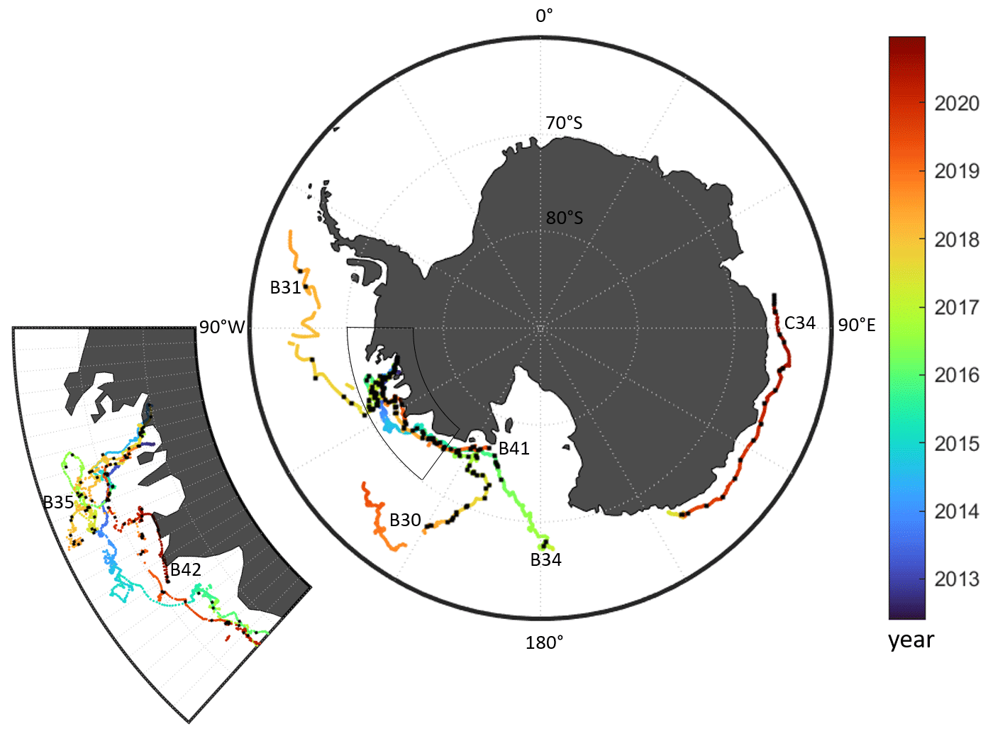
Figure 1 Spatial and temporal coverage of our dataset. The trajectories (by Budge and Long, 2018) of the seven selected icebergs are colour-coded according to time and the black squares indicate the locations of the images used in this study.

2.2 Grouping of input images according to environmental conditions

We visually group all input images into different categories to assess the performance in different potentially challenging conditions. These groups are open ocean, sea ice, fragments, other icebergs, coast and dark icebergs (Fig. 2 shows one example of each). We class an image as dark iceberg if the iceberg appears as dark or does not stand out from the background (Wesche and Dierking, 2012). Images are grouped into the coast category if they contain nearby ice shelves or glaciers on the Antarctic continent. Due to very similar physical conditions, ice shelves and icebergs are hard to differentiate. The category of other icebergs was introduced, because in some cases, several giant icebergs drift very close to each other and are (partially) visible in our cropped images. If another iceberg of similar size is present, the algorithms might pick the wrong iceberg and we class such images as other icebergs. There is also one case where a bigger iceberg is partially visible, but we are aiming to segment the largest iceberg that is fully visible (Fig. 5h). We assign images to the fragments category if they exhibit fragments close to the iceberg. Fragments occur frequently in the vicinity of icebergs, as icebergs regularly calve smaller fragments around their edges. When the fragments are close to the main iceberg, they are easily grouped together (Koo et al., 2021). The last challenge is sea ice. Young and flat sea ice usually appears homogenous and dark, meaning it does not pose a problem. However, older, ridged sea ice and other cases where the background appears grey rather than black with significant structure (Mazur et al., 2017) are grouped into this category. Images are grouped into the open ocean category if no obvious challenge is apparent to us. This includes cases where the sea ice is not visually apparent (i.e. young and flat) and the background appears as dark and relatively homogenous or where fragments are further away from the iceberg. If several challenges are present (e.g. if coast and sea ice are visible), we assign the image to the most relevant group. Table 3 gives the number of images per category.

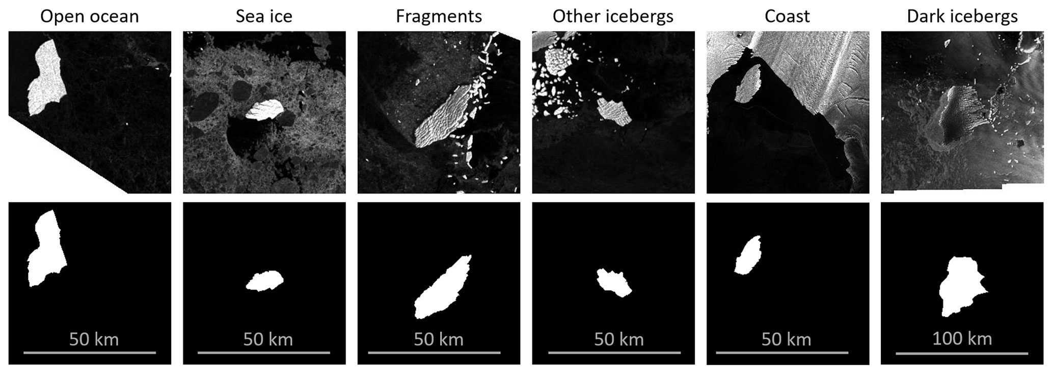
Figure 2 Examples of input images (top row) and segmentation maps based on manually derived delineations (bottom row) in different environmental conditions. From left to right these are B31 in open ocean, B41 surrounded by sea ice, B42 with nearby fragments, C34 and another similar sized iceberg, B41 close to the coast and B30 appearing dark.

2.3 Manual delineation of iceberg perimeters

Although the goal is to develop an automated segmentation technique, manual delineations of iceberg extent are required to train the U-net and for the evaluation of all methods. We manually digitise the iceberg perimeter in all 191 images using Geographic Information System (GIS) software to yield a polygon. The accuracy of such manual delineations is estimated to be 2 %–4 % of the iceberg area (Bouhier et al., 2018; Braakmann-Folgmann et al., 2021, 2022). We then create a binary map of the same size as the input image, where pixels within the manually derived polygon are defined as iceberg and everything else as background, to allow a rapid evaluation of performance. Fig. 2 shows some examples of input images and their corresponding segmentation maps based on the manual outlines. We regard the manually derived outlines as the most accurate. Therefore, we use these binary maps to train our neural network and to evaluate all automated segmentation techniques. When the area deviation of our automated segmentation techniques drops below 2 %–4 %, their prediction might be more accurate than the manual delineation. In any case, automated approaches are advantageous over manual delineations – especially when rolled out for numerous icebergs or in operational applications – as each outline takes several minutes to digitise manually.

3 Methods

This section describes the implementation of two standard segmentation methods and our U-net architecture. We also introduce the different performance metrics used to evaluate our results.

3.1 Iceberg segmentation with k-means and Otsu thresholding

We implement two standard segmentation techniques as a baseline: Otsu thresholding and k-means. In both cases, we mask out the areas that had no satellite scene coverage by setting them to zero (black). For the first segmentation technique, we smooth the input image with a 5×5 Gaussian kernel. Then we apply the Otsu threshold (Otsu, 1979), yielding a binary image. The Otsu threshold is determined automatically based on the grey-scale histogram of the image so that the within-class variance is minimised. To find an iceberg, we apply connected component analysis to the binary image and select the largest component. We also experimented with other thresholding techniques including adaptive mean and adaptive Gaussian thresholding, but we found that the Otsu threshold gave the best results (for the B42 iceberg we found F₁ scores of 0.58, 0.67 and 0.84). Although different thresholding techniques have been proposed for iceberg detection (Frost et al., 2016; Mazur et al., 2017; Power et al., 2001; Wesche and Dierking, 2012; Willis et al., 1996), to our knowledge none of them have used the Otsu method. The second technique is k-means (Macqueen, 1967), with k=2. K-means is a clustering technique which divides the data into k clusters iteratively. The initial cluster centres are chosen randomly and each observation is assigned to the nearest cluster. Then, in each iteration, new centroids (means) are calculated per cluster and all observations are assigned to the nearest cluster again. We run the algorithm for 20 iterations. We also repeat this 50 times with different initialisations and take the result with the best compactness. Afterwards, we perform a connected component analysis and select the largest component. K-means and a variation of it have also been applied to track selected icebergs by Collares et al. (2018) and Koo et al. (2021), respectively. Both our standard segmentation techniques are implemented using the OpenCV library (Bradski, 2000) for Python.

Figure 3 Modified U-net architecture as used in this paper.

3.2 Iceberg segmentation with U-net

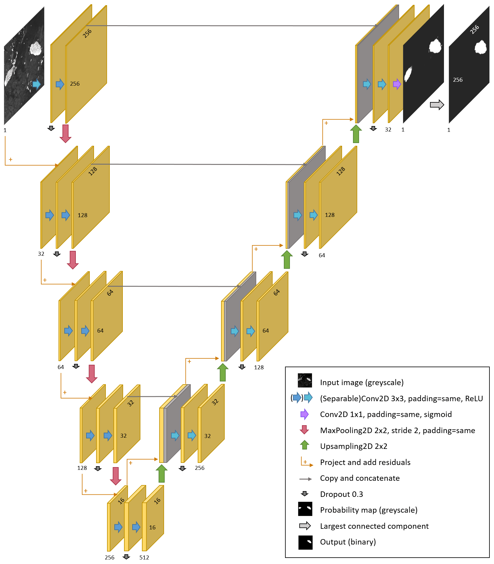
We implement a U-net architecture to segment Sentinel-1 input images into the largest iceberg and background, which is based on the original U-net (Ronneberger et al., 2015) with some modifications. The input images are 256 × 256 one-channel backscatter images (as Sect. 2.1. describes and Fig. 2 shows). The U-net is composed of an encoder that produces a compressed representation of the input image and a decoder that constructs a segmentation map from the compressed encoding with the same spatial resolution as the input (Fig. 3). The encoder uses a number of convolutional and pooling layers to generate feature maps at increasing levels of abstraction and spatial scale. The decoder uses further convolutional layers and upsampling to construct the required segmentation map. Cross-links convey feature maps from different spatial scales in the encoder to the respective decoder stage, where they are combined with contextual feature maps from the decoder layer below. This allows U-net to produce accurate segmentations whilst also considering contextual features. We use padding in the convolutions and pooling operations, so that the feature maps remain the same size as the input at each level (spatial scale) and are reduced by 50 % in height and width between encoder levels. We also use depth-wise separable convolutions (Chollet, 2017), which are more efficient. Furthermore, we added a dropout of 0.3 in between the two convolutions per level to avoid overfitting (Srivastava et al., 2014). We also added residual connections to aid the learning process and increase the accuracy (He et al., 2016). The outputs are one-channel 256 × 256 arrays, representing the probability that each pixel belongs to the iceberg class. During training, these output maps are compared with the segmentation maps from our manually derived outlines to alter the network parameters accordingly. When evaluating the validation and test data output, we convert the probability map to a binary output, where 1 corresponds to the iceberg class and 0 corresponds to the background (everything else), by thresholding it at 0.5. As we are only interested in the largest iceberg, smaller icebergs and iceberg fragments are removed by also applying a connected component analysis and selecting the largest component (Fig. 3).

We train and evaluate the network using cross-validation. This means that we train seven different neural networks and always retain the images of one iceberg for testing as an independent dataset. In the end, it allows us to evaluate the performance of our U-net across all seven icebergs, as each of them is used as (unseen) test data for one of the networks. The exact number of test images varies, as we have between 15 and 46 images per iceberg (Table 2). Although the images are roughly 1 month apart and cover a wide range of seasons and surroundings overall (e.g. near the calving front, surrounded by sea ice and within open ocean), we find that consecutive images of the same iceberg are often similar – concerning iceberg shape, size and appearance as well as the surrounding. Therefore, we do not mix training and test data. On the other hand, and for the same reason, we find that it stabilises the training process if we draw training and validation data from the same set of icebergs. To determine when to stop the learning process to avoid overfitting, we use 24 images as validation data. Depending on which iceberg was picked for testing, this leaves between 121 and 152 images for training. Other hyperparameters like network architecture, number of layers, optimiser, initial learning rate, loss function and batch size are the same for all seven networks and were set using the B42 iceberg as test data. We also tried to augment the data by flipping the training images vertically and horizontally, leading to a tripling of the training data, but we found a slightly degraded performance (F₁ score for the B42 iceberg used as test data is reduced from 0.88 to 0.79). We believe that this is because consecutive images already show a similar iceberg shape and size in similar conditions, but with varying rotation and translation through the natural drift. Therefore, in this case data augmentation does not help but rather leads to overfitting. We train the networks end-to-end using a binary cross-entropy loss function and a batch size of 1. Higher batch sizes had little impact on the performance and run time. The Adam optimiser (Kingma and Ba, 2015) is employed with an initial learning rate of 0.001. The learning rate is halved when the validation loss has not decreased for eight consecutive epochs. Training is stopped when the validation loss has not improved for 20 epochs. In practice, this means that the networks are trained for 57–193 epochs. The implementation is done in Python using Keras (Chollet et al., 2015). Training takes up to 20 min on a Tesla P100 GPU with 25 GB RAM (Google Colab Pro). Once trained, U-net can be applied without any user intervention and the prediction for 24 images takes 0.2 s.

3.3 Performance metrics

We evaluate the performance of the three methods compared with the manual delineations using a range of metrics. True positives (TP) are all correctly classified iceberg pixels and true negatives (TN) are all correctly classified background pixels. False positives (FP) are pixels that were classified as iceberg pixels but belong to the background according to manual delineations. And false negatives (FN) are iceberg pixels in the manually derived segmentation map, which the algorithm has missed and erroneously classified as background. These are the bases for most evaluation metrics including the overall accuracy, the F₁ score (also known as dice coefficient), misses (also known as the false negative rate) and false alarms (also known as the false positive rate). The detection rate is equal to the iceberg class accuracy and can be derived from 1 minus the misses; hence, we do not list it separately. The F₁ score is a number between 0 and 1, where 1 is best and means that the model can successfully identify both positive and negative examples. In the case of a large class imbalance, the F₁ score is much more meaningful than the overall accuracy. The iceberg class makes up only 5 % of all pixels, so we focus on the F₁ score but list the overall accuracy for completeness. Except for the F₁ score, all measures are given in percentages. In addition to these metrics commonly used to evaluate segmentation algorithms, we also examine the accuracy of the resulting area estimates a_i. We calculate the mean absolute error (MAE) in area, the mean error (area bias) and the median absolute deviation (MAD) in area. We focus on the MAD, as it is robust to a few complete failures. However, some previous studies (Barbat et al., 2021; Mazur et al., 2017) have reported the MAE in area but most (Silva and Bigg, 2005; Wesche and Dierking, 2012, 2015; Williams et al., 1999) have reported the area bias, so we also list these for completeness. Areas a_i and α_i are calculated as the sum of all iceberg pixels in the prediction and manually derived segmentation map, respectively, multiplied by the pixel area (240 × 240 m or 480 × 480 m). All area deviations are relative deviations and given as percentages compared with the iceberg area in the manually derived segmentation map. Due to the large size range (54–1052 km²), relative numbers are more meaningful. We also calculate the standard deviation for each metric. Only the MAD is given with the 25 % and 75 % quantiles instead.

$$\begin{array}{}\text{(1)}& {\displaystyle }{F}_{\mathrm{1}}={\displaystyle \frac{\mathrm{2}\mathrm{TP}}{\mathrm{2}\mathrm{TP}+\mathrm{FN}+\mathrm{FP}}}\text{(2)}& {\displaystyle }\text{Overall accuracy}={\displaystyle \frac{\mathrm{TN}+\mathrm{TP}}{\mathrm{TN}+\mathrm{TP}+\mathrm{FN}+\mathrm{FP}}}\text{(3)}& {\displaystyle }\text{Misses}={\displaystyle \frac{\mathrm{FN}}{\mathrm{FN}+\mathrm{TP}}}\text{(4)}& {\displaystyle }\text{False alarms}={\displaystyle \frac{\mathrm{FP}}{\mathrm{FP}+\mathrm{TN}}}\text{(5)}& {\displaystyle }\mathrm{MAE}={\displaystyle \frac{\mathrm{1}}{n}}\sum _{i=\mathrm{1}}^n{\displaystyle \frac{\mathrm{|}{a}_i-{\mathit{\alpha }}_i\mathrm{|}}{{\mathit{\alpha }}_i}}\text{(6)}& {\displaystyle }\text{Area bias}={\displaystyle \frac{\mathrm{1}}{n}}\sum _{i=\mathrm{1}}^n{\displaystyle \frac{a_i-{\mathit{\alpha }}_i}{{\mathit{\alpha }}_i}}\text{(7)}& {\displaystyle }\mathrm{MAD}=\mathrm{median}\left({\displaystyle \frac{\left|a_i-{\mathit{\alpha }}_i\right|}{{\mathit{\alpha }}_i}}\right)\end{array}$$

4 Results and discussion

In this section, we present and discuss the results from the three different approaches (U-net, Otsu and k-means). The best visualisation of the results can be found in the supplementary animations (Braakmann-Folgmann, 2023), showing all 191 images with the predicted iceberg outlines from all methods plotted on top. There is one animation per iceberg. Our analysis in the following is based mainly on statistics, but we also show some examples to allow for a visual, qualitative assessment. After an overall analysis, we assess the performance of the approaches on each iceberg and evaluate the impact of the iceberg size and different environmental conditions in the scenes. Finally, we compare our results to previous studies.

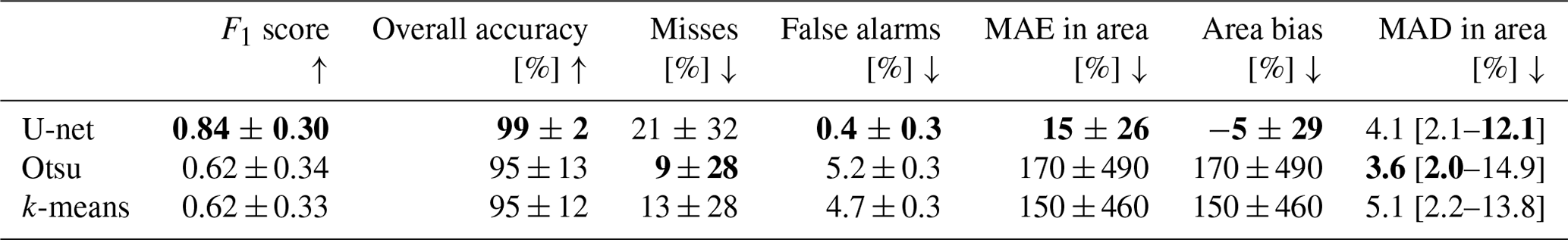
Table 1 Performance metrics with standard deviations of U-net, Otsu and k-means across all test datasets (191 images). The median absolute area deviation (MAD) is given with 25 % and 75 % quantiles instead of standard deviation. Arrows indicate whether high (up) or low (down) numbers are desirable. The best score per metric is highlighted in bold.

4.1 Performance of the three methods

Comparing the performance of all three techniques, we find that U-net outperforms Otsu and k-means in most metrics. It achieves a significantly higher F₁ score (0.84 compared to 0.62, Table 1) and generates much fewer false alarms (0.4 % instead of 4.7 % and 5.2 %). On the other hand, both standard segmentation methods have fewer misses than U-net (9 % and 13 % compared to 21 %). On this metric Otsu scores the best. In terms of iceberg area, the predictions by U-net are much closer to the manually derived outlines in terms of MAE and bias. Otsu and k-means clearly suffer from a few total failures with over 100 % deviation which bias these metrics in their cases. The MAD, which is less sensitive to such outliers, is similar for the three methods, with Otsu scoring the best (3.6 %), followed by U-net (4.1 %) and k-means (5.1 %). The 25 % quantiles are very similar for all three methods (2.0 %, 2.1 % and 2.2 %, respectively). On the 75 % quantiles, U-net achieves slightly better results (12.1 % area deviation, compared to 13.8 % and 14.9 % for k-means and Otsu, respectively). This means that 75 % of all U-net predictions deviate from the manually derived area by 12.1 % or less. Overall, U-net scores better in most categories but tends to miss parts and misclassify iceberg pixels as background.

4.2 Impact of iceberg size

Next, we evaluate how U-net performs for each of the seven different giant icebergs (Table 2, shaded in grey and Fig. 4) to assess the impact of the chosen test dataset and different iceberg sizes. Here, we find that B34 gives the best results. The number of images for this iceberg is the smallest (15 images), meaning that there are more images left for training and the background is usually not too challenging. B41 gives the lowest F₁ score. This dataset is the largest one, containing 46 images, and hence leaves the lowest number of images for training. Furthermore, B41 remains in close proximity to its calving position for over a year, which means that the first 13 images contain a significant amount of coast – often directly next to the iceberg (see Fig. 4's first three images or the supplementary animation for all images). In these cases all techniques pick the coast rather than the iceberg (as discussed later). The highest MAD and miss rate occur for iceberg B31. Because the images of B30 – our largest iceberg – are resized, this means that B31 appears largest in the images. Therefore, we believe that the large size of the iceberg, which U-net has not seen in the training data, causes U-net to miss parts of the iceberg (Figs. 4 and 5b, f). This is supported by the fact that U-net misses large parts of B31 in the beginning (first few images in Fig. 4) then misses smaller parts, and once the iceberg has decreased to a size similar to other icebergs, U-net is suitable (last four images of B31 in Fig. 4). In general, we find quite variable performance depending on which iceberg is retained as test data. This is because the same challenges (e.g. iceberg size, shape and surrounding) occur in subsequent images of the same iceberg, even when they are 1 month apart (best seen in the supplementary animations). It is also the reason why we decided to evaluate the methods using cross-validation, as this makes the analysis less sensitive to the choice of a single iceberg as test data.

Table 2 Performance of the three methods for each test dataset (iceberg). The number of images per iceberg and their minimum and maximum size are also given. Note that most images of B30 are rescaled, so it appears smaller in the images. Arrows indicate whether high (up) or low (down) numbers are desirable. The best scores per iceberg and metric are highlighted in bold.

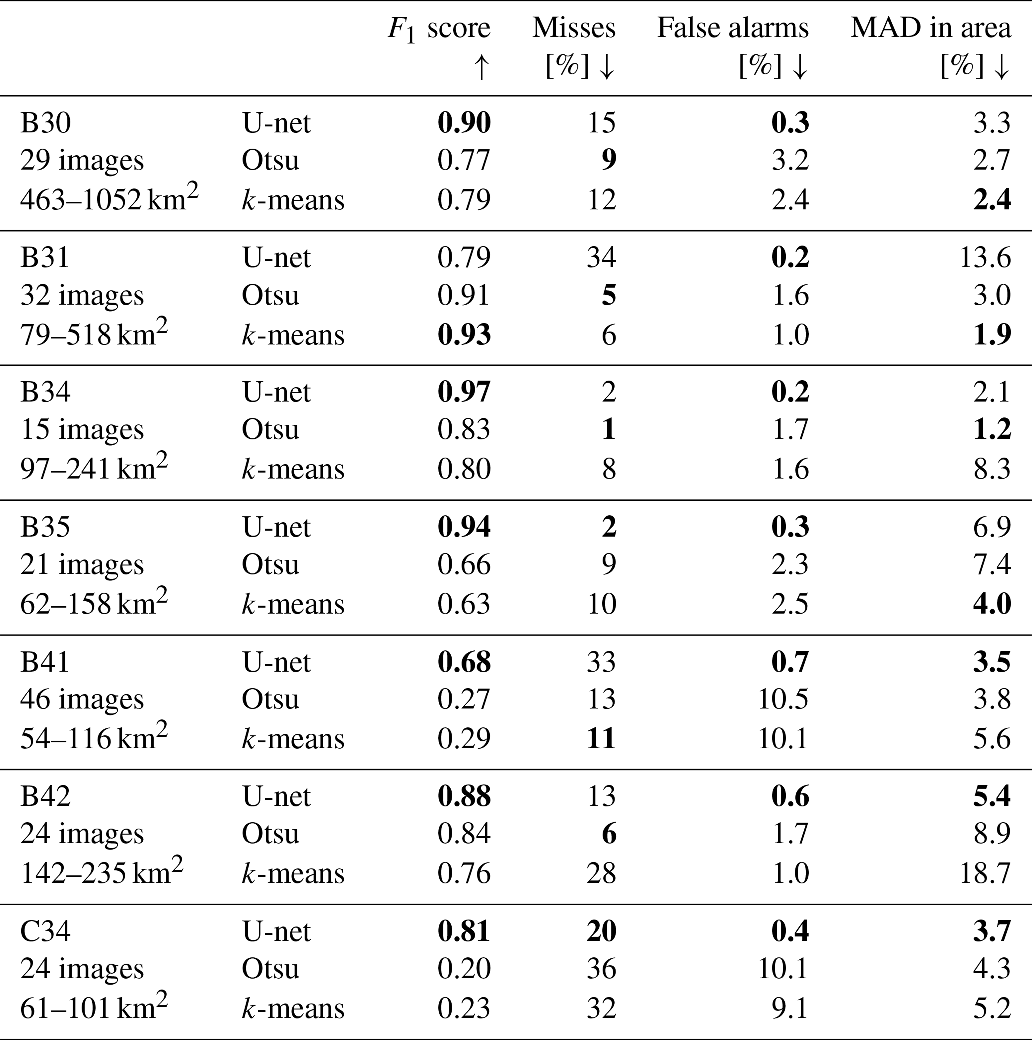
Also for Otsu and k-means the performance varies a lot depending on which iceberg is chosen as test data. The F₁ scores for Otsu range from 0.20–0.91, being the lowest for C34 and the highest for B31. Similarly, k-means also reaches the lowest F₁ score of 0.23 for C34 and the highest F₁ score of 0.93 for B31. Compared to that, U-net is more consistent, reaching F₁ scores between 0.68 and 0.97, but still exhibits significant variability. The fact that Otsu and k-means score so well for B31 also indicates that this dataset is not hard per se. We rather suspect that we are challenging U-net too much when the iceberg in the test data is bigger than any iceberg in the training data. Neural networks are known to struggle with a domain shift, where the test data are from a shifted version of the training data distribution, and even more with out-of-domain samples from outside the training data distribution (Gawlikowski et al., 2021). Both are caused by insufficient training data, not or barely covering these examples. Therefore, we recommend expanding the training data before operationally applying U-net to icebergs larger than those covered by the current training dataset. In contrast, iceberg B41, where U-net reaches the lowest F₁ score, poses an even greater problem to the other algorithms, meaning that this dataset is actually challenging. Finally, we observe that U-net achieves the lowest false alarm rate for each iceberg. Otsu generates the most false alarms (highest rate for six out of seven icebergs) but also achieves the lowest miss rate for four out of seven icebergs. Except for B31, U-net consistently achieves the highest F₁ score. In terms of MAD in area k-means and U-net score the best for three out of the seven icebergs each.

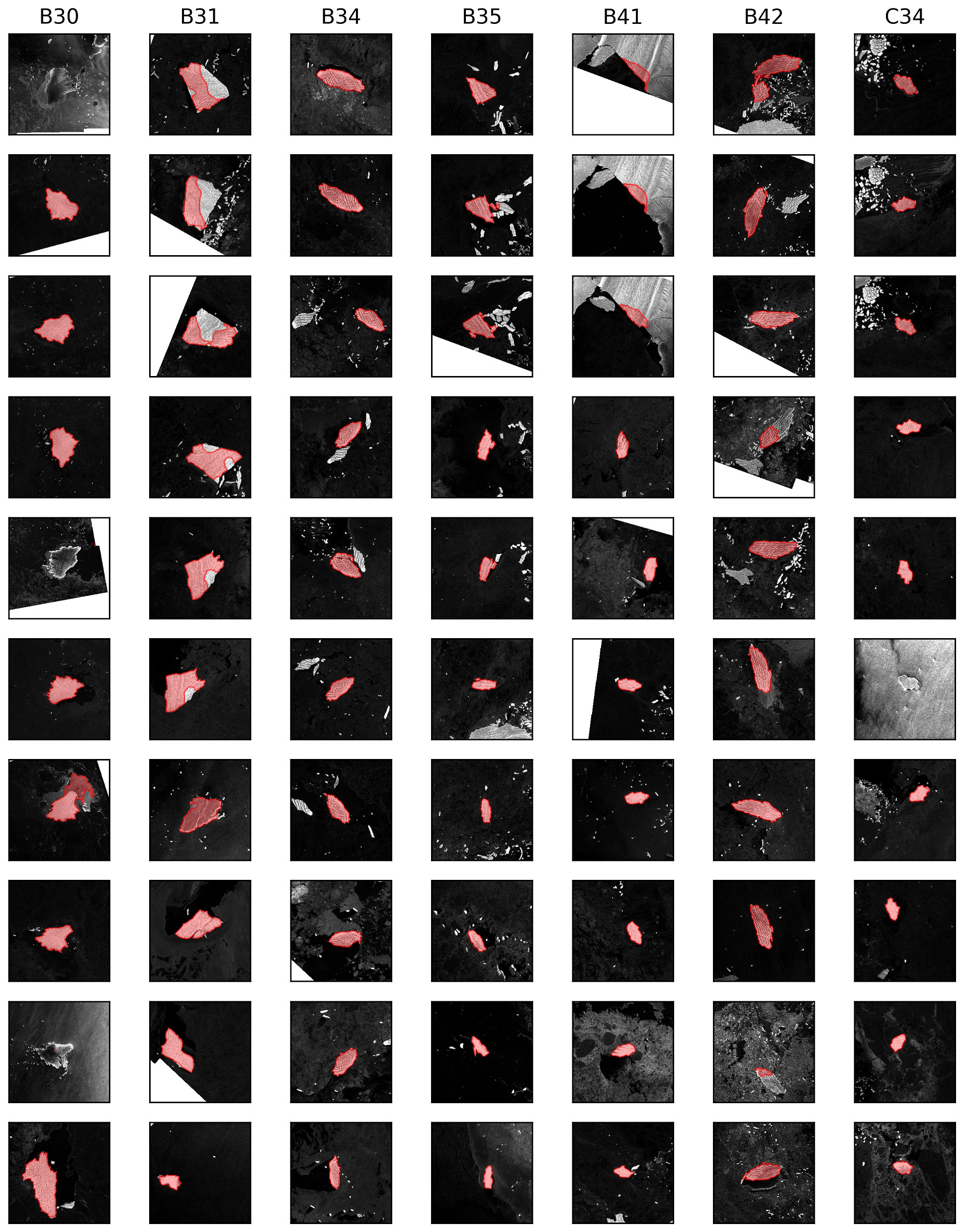
Figure 4 U-net-derived iceberg outlines (red) plotted on top of the input images for 10 images per iceberg (columns). We always include the first and last image from each time series and sample the others equally in between. As the number of images per iceberg ranges from 15–46, this means that the images of B34 are 1–2 months apart, while the images for B41 are 5 months apart in this figure. The full time series and results of all methods can be viewed in the supplementary animations (one per iceberg).

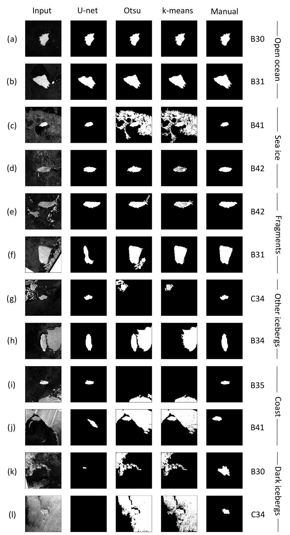
Figure 5 Examples of input images (first column) and segmentation maps generated by U-net (second column), Otsu (third column), k-means (fourth column) and manual delineations (last column). We picked these images for illustration to cover each category of environmental conditions twice and to include all icebergs (labelled on the right).

4.3 Impact of different environmental conditions

Grouping the images according to the surrounding environmental conditions (see Sect. 2.2.) allows us to judge how well each method can deal with the respective challenge (Fig. 5, Table 3). Open ocean makes up most of the images (46 %) and all methods perform very well with F₁ scores of 0.93–0.95 and MAD in area of 2.4 %–3.2 %. The Otsu threshold performs the best, but the differences between the methods are very small. The two sample images (Fig. 5a, b) also illustrate that the only problem in this category is that U-net generally tends to miss parts of B31 rather than open ocean in itself posing a problem.

Sea ice occurs in 14 % of our images. Overall, U-net achieves the best F₁ score (0.88 compared to 0.72 and 0.74), but the Otsu threshold gives a slightly better MAD in area (4.3 % rather than 4.8 % and 5.4 %). Visually, the U-net predictions seem to be the most robust, as sea ice is discarded reliably. In contrast, the two other methods sometimes connect patches of sea ice to the iceberg (Fig. 5c) but also work fine in other cases (Fig. 5d).

Table 3 Performance of the three methods in different environmental conditions. The first column also indicates how often these conditions occur in our dataset. Arrows indicate whether high (up) or low (down) numbers are desirable. The best values per category and metric are highlighted in bold.

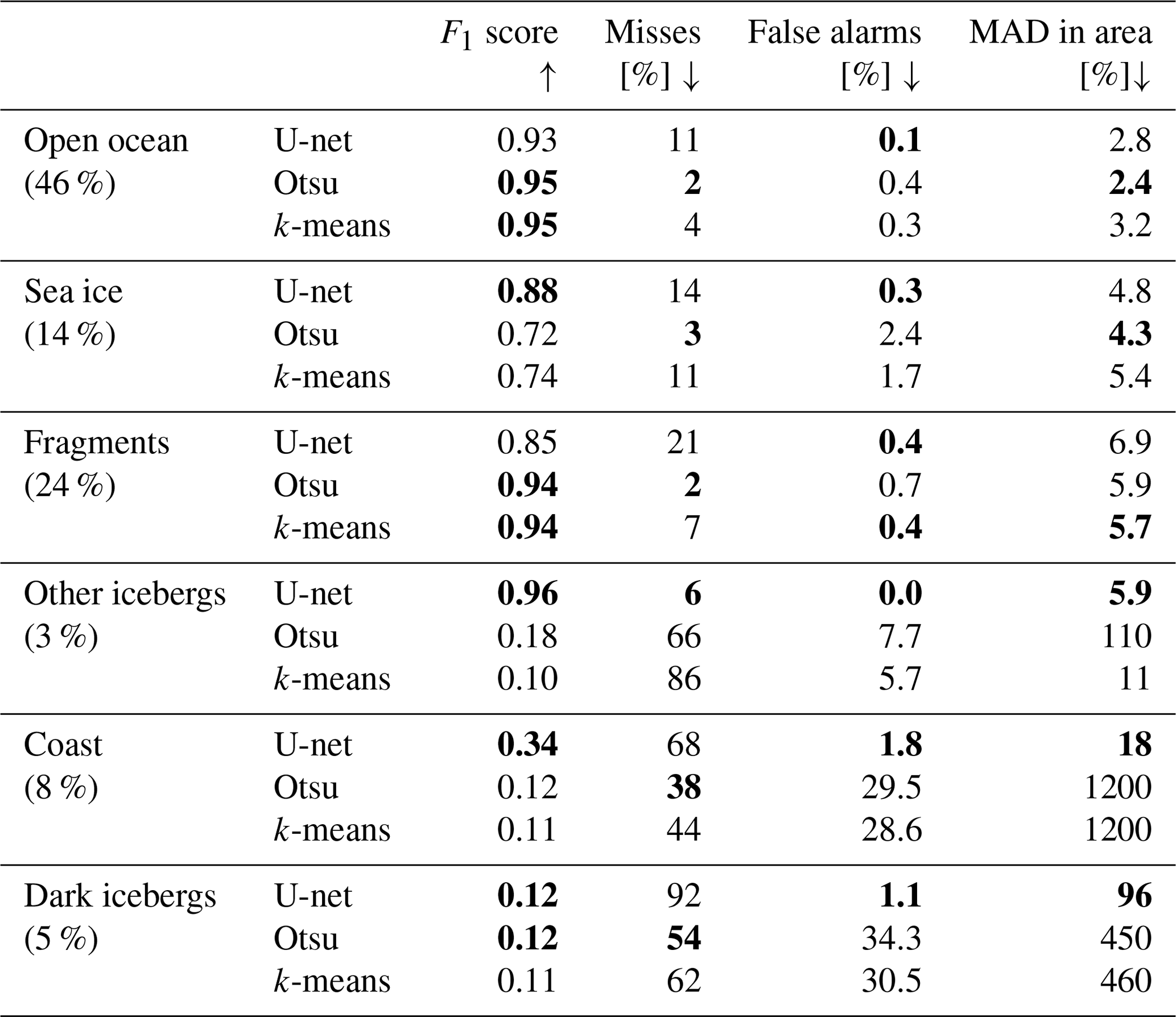
Iceberg fragments drifting in direct proximity to the target iceberg were found in 24 % of our images. Overall, k-means scores best in this category with a MAD of 5.7 % compared with 5.9 % and 6.9 %. In terms of the F₁ score, Otsu and k-means both reach 0.94, whereas U-net only reaches 0.85. Visually, there are a few instances where Otsu connects more fragments to the iceberg than k-means and U-net (Fig. 5e, f). This might be due to the Gaussian smoothing that we apply before the thresholding. We do not apply this step before k-means and find that k-means tends to rather oversegment images, leaving small holes on the inside (Fig. 5d, e). However, in the case of fragments, this turns out to be beneficial, as it allows k-means to reliably separate fragments from icebergs, even when they are very close by. The problem for U-net does not seem to be the actual fragments themselves, as it rarely connects any fragments to the iceberg (Fig. 5e, f). However, the images containing fragments are mostly from the large B31 and B42 icebergs, where U-net struggles due to their large extent. This can also be seen from the fact that U-net and k-means both only generate 0.4 % false alarms (fragments erroneously connected to the iceberg), but U-net has a much higher miss rate.

In 3 % of all images, another similar sized or bigger iceberg is (partially) visible. U-net scores the best in all categories, by a large margin, yielding an F₁ score of 0.96 compared to 0.12 and 0.11 and a MAD in area of 5.9 % compared to 11 % and 110 %. Visually, it also becomes clear that U-net reliably picks the target iceberg and discards any other ice, while Otsu and k-means often pick the wrong iceberg or connect the iceberg with other ice (Fig. 5g, h). However, considering iceberg shape and size in a tracking scenario could help mitigate this phenomenon (Barbat et al., 2021; Collares et al., 2018; Koo et al., 2021).

The coast is present in 8 % of all images and U-net outperforms the other techniques but also struggles in certain cases. The F₁ score is 0.34 for U-net and 0.12 and 0.11 for Otsu and k-means, respectively. While U-net achieves a MAD of 18 %, the other methods yield over 1000 % each. Figure 5j illustrates what is happening in these cases. If too much coast is present, all algorithms pick the coast rather than the iceberg (and this is much larger than the iceberg, hence 1000 % deviation). However, U-net discards smaller parts of the coast around the image edges (Fig. 5i). On the one hand, this is because of the sliding convolution window and, on the other hand, because U-net learns that the iceberg is usually in the centre (as we crop the images around the estimated position from operational iceberg tracking databases). Hence, U-net is able to correctly pick out the iceberg if not too much coast is present. For the same reason, it is easier for U-net to discard other icebergs at the image edges. Interestingly, even when a lot of coast is present, U-net does not pick the full coast but predicts either nothing or a small – almost iceberg-shaped – part of the coast (Fig. 5j). This could indicate that U-net even learns that only ice that is fully surrounded by water is an iceberg. A possible strategy to avoid misclassifications due to large amounts of coast would be the inclusion of a land mask (Barbat et al., 2019a; Collares et al., 2018; Frost et al., 2016; Mazur et al., 2017; Silva and Bigg, 2005). However, ice shelves and glaciers advance and retreat regularly; especially the calving of icebergs themselves significantly alters the land mask. Thus, just after calving, the iceberg would be within the former land mask and would not be picked up. A potential solution could be to always use the latest frontal positions from Baumhoer et al. (2023) as a dynamic land mask.

The last category of dark icebergs is the hardest and makes up 5 % of the overall dataset. In these cases, all methods fail with F₁ scores of 0.11–0.12 and the lowest MAD in area of 96 %. Again, it is interesting that U-net predicts either very small patches or nothing at all in these cases (Fig. 5k, l), while the other two methods segment large areas of brighter-looking ocean. Potentially, U-net could learn to segment dark icebergs with a lot more training examples, but we only had 10 such images in our overall dataset. Finally, we would like to stress that the occurrence of these different environmental conditions will vary and our dataset is not necessarily representative of all icebergs. We also find that the influence of iceberg size and environmental conditions cannot always be disentangled, as subsequent images of the same iceberg are often similar and the different environmental conditions are not spread equally across the different test datasets (individual icebergs). Therefore, the fact that U-net misses parts of B31 also impacts its performance in mainly the fragments and open ocean category. Apart from these misses, U-net scores at least as well as the other methods in the open ocean and fragments categories (lower or same false alarm rate) and outperforms them in the sea ice, other icebergs and coast categories. Dark icebergs and larger areas of coast remain a problem for all methods.

4.4 Comparison with previous studies

Previous studies state different accuracy measures. And due to the slightly different goal of detecting all icebergs in a scene rather than finding one giant iceberg and accurately predicting its outline and area, they are not directly comparable. Two studies employ the k-means algorithm (Collares et al., 2018) or a variation of it (Koo et al., 2021), so we have indirectly compared U-net to them, though none of them report any of our accuracy measures. Many of the previous approaches rely on some form of thresholding (Frost et al., 2016; Gill, 2001; Mazur et al., 2017; Power et al., 2001; Wesche and Dierking, 2012; Willis et al., 1996). We somehow covered these methods by comparing U-net to the Otsu threshold, but the exact approaches vary and none of them have applied the Otsu threshold. Two of the threshold-based methods report estimates for their area deviations. Wesche and Dierking (2012) state that the iceberg area was overestimated by 10 ± 21 % with their approach. In a following study, they find that for the correctly detected icebergs 13.3 % of the total area was missing (Wesche and Dierking, 2015), meaning a bias in the opposite direction. Mazur et al. (2017) find positive and negative area deviations of ±25 % on average. For edge-detection-based algorithms, Williams et al. (1999) find an overestimation of the iceberg area by 20 % and the approach of Silva and Bigg (2005) yields an underestimation of the iceberg area by 10 %–13 %. Again, these are biases and both approaches are limited to winter images. For U-net, we find a bias of −5.0 ± 29.1 %, which is lower than previous studies. But it comes with a relatively high standard deviation due to some complete failures where the iceberg is not found at all. Previous studies only compare iceberg areas where icebergs were detected successfully. Barbat et al. (2019a) report the lowest false positive (2.3 %) and false negative (3.3 %) rates and the highest overall accuracy (97.5 %) of all previous studies. While their false negative rate is lower than our false negative rate (21 %), U-net achieves a lower false positive rate of 0.4 % and a higher overall accuracy of 99 %. In a second study, Barbat et al. (2021) also analyse the area deviation of the detected icebergs and find average area deviations of 10±4 %, which is also the best score reported so far, though they only consider correctly detected icebergs in this metric. We find an MAE of 15±26 % for U-net, which is slightly higher, but it contains images where the iceberg was not found at all. These cases are not included in the estimates of Barbat et al. (2021). Our MAD, which is less sensitive to such outliers, is 4.1 %, with 25 % and 75 % quantiles of 2.1 % and 12.1 %, respectively. These metrics compare favourably to all previous studies. We also demonstrate in our study that the performance varies depending on the chosen test dataset; therefore, all measures and comparisons can only give an indication of the real performance. Judging from the data we have and comparing our results on this with previous studies as well as possible, U-net proves to be a very promising approach.

Qualitatively, previous studies have found degraded accuracies in challenging environmental conditions or excluded these from their datasets. Some studies report false detections due to sea ice (Koo et al., 2021; Mazur et al., 2017; Wesche and Dierking, 2012) or only applied their algorithm to sea-ice-free conditions (Willis et al., 1996). Moreover, several previous studies have also encountered problems with clusters of several icebergs and iceberg fragments too close to each other (Barbat et al., 2019a; Frost et al., 2016; Koo et al., 2021; Williams et al., 1999). U-net also shows slightly degraded performance in these situations (4.8 % and 6.9 % MAD in area, respectively, compared with 2.8 % in open ocean and F₁ scores of 0.88 and 0.85, respectively, compared with 0.93) but still achieves satisfying results in most of these cases. The challenge of other big icebergs does not occur in previous studies, since they were looking for all icebergs anyway. In terms of the coast, many previous studies have employed a land mask (e.g. Barbat et al., 2019a; Collares et al., 2018; Frost et al., 2016; Mazur et al., 2017; Silva and Bigg, 2005) but might miss newly calved icebergs due to that. Finally, the problem of dark icebergs has been described in several papers (Mazur et al., 2017; Wesche and Dierking, 2012; Williams et al., 1999) but was rarely mentioned in the evaluation. This is likely because most previous studies use visual inspection to identify misses and false alarms (e.g. Barbat et al., 2019a; Frost et al., 2016; Mazur et al., 2017; Wesche and Dierking, 2012; Williams et al., 1999). However, dark icebergs are hard to spot in SAR images even for manual operators. They might be missed by the visual inspection too unless, such as in our case, we know that there must be an iceberg of a certain size and shape that we are looking for. Others limit their method to winter images, when dark icebergs do not occur (Silva and Bigg, 2005; Williams et al., 1999; Young et al., 1998).

5 Conclusions

We have developed a novel algorithm to automatically segment giant Antarctic icebergs in Sentinel-1 images. It is the first study to apply a deep neural network for iceberg segmentation. Furthermore, it is also the first study specifically targeting giant icebergs. Comparing U-net to two state-of-the-art segmentation techniques (Otsu thresholding and k-means), we find that U-net outperforms them in most metrics. Across all 191 images, U-net achieves an F₁ score of 0.84 and a median absolute area deviation of 4.1 %. Only the miss rates of Otsu and k-means are lower than for U-net, as we find that U-net overlooks parts of the iceberg appearing largest in the images. In this case, all training samples show smaller icebergs. We believe that this issue could be resolved with a larger training dataset. U-net can reliably handle a variety of challenging environmental conditions including sea ice, nearby iceberg fragments, other icebergs and small patches of nearby coast, though it fails when too much coast is visible and when icebergs appear dark. In these cases, all existing algorithms fail, but such obvious errors could easily be picked out in a tracking scenario. Compared to previous studies, we also regard our results as promising. In the short term, further post-processing could be implemented to filter outliers for an operational application. But in the long run, we would suggest enlarging the training dataset before applying it to icebergs that are smaller or larger than those currently covered by the training data.