the Creative Commons Attribution 4.0 License.
the Creative Commons Attribution 4.0 License.
 | 21 Sep 2023
New estimates of pan-Arctic sea ice–atmosphere neutral drag coefficients from ICESat-2 elevation data
Alexander Mchedlishvili
Christof Lüpkes
Alek Petty
Michel Tsamados
Gunnar Spreen
The effect that sea ice topography has on the momentum transfer between ice and atmosphere is not fully quantified due to the vast extent of the Arctic and limitations of current measurement techniques. Here we present a method to estimate pan-Arctic momentum transfer via a parameterization that links sea ice–atmosphere form drag coefficients with surface feature height and spacing. We measure these sea ice surface feature parameters using the Ice, Cloud and land Elevation Satellite-2 (ICESat-2). Though ICESat-2 is unable to resolve as well as airborne surveys, it has a higher along-track spatial resolution than other contemporary altimeter satellites. As some narrow obstacles are effectively smoothed out by the ICESat-2 ATL07 spatial resolution, we use near-coincident high-resolution Airborne Topographic Mapper (ATM) elevation data from NASA's Operation IceBridge (OIB) mission to scale up the regional ICESat-2 drag estimates. By also incorporating drag due to open water, floe edges and sea ice skin drag, we produced a time series of average total pan-Arctic neutral atmospheric drag coefficient estimates from November 2018 to May 2022. Here we have observed its temporal evolution to be unique and not directly tied to sea ice extent. By also mapping 3-month aggregates for the years 2019, 2020 and 2021 for better regional analysis, we found the thick multiyear ice area directly north of the Canadian Archipelago and Greenland to be consistently above , while most of the multiyear ice portion of the Arctic is typically around .
- Article
(19609 KB) - Full-text XML
- BibTeX
- EndNote


Arctic sea ice is heterogeneous with respect to several characteristics, including its concentration, thickness and roughness (e.g., Thorndike et al., 1975; Bourke and Garrett, 1987). The understanding of how these parameters vary with space and time is important for several reasons, including its impact on human activities, e.g., navigation, and its impact on the physical system, e.g., the transfer of momentum and energy between the atmosphere and ocean.
Studies of Arctic sea ice have arguably focused more on constraining variability in concentration and thickness towards estimating sea ice volume and its variability in time and space. However, the surface roughness of sea ice also exhibits strong spatial and temporal variability (e.g., Andreas et al., 2010; Lüpkes et al., 2012; Castellani et al., 2014; Petty et al., 2017) that needs to be better understood. Surface roughness can be related to the neutral drag coefficient by applying the Monin–Obukhov theory. Since the roughness length for momentum and the scalar roughness length for heat and moisture also occur in the non-neutral transfer coefficients, surface roughness directly impacts not only momentum transport but also the transfer of heat and moisture between the atmosphere and the underlying surface. Rougher surfaces can create more turbulence and enhance mixing, thereby influencing the stability of the atmospheric boundary layer (e.g., Garratt, 1992; Schneider et al., 2022; Lüpkes and Gryanik, 2015). Due to its impact on momentum and heat transport over and below the sea ice layer, surface roughness is a fundamental parameter influencing the distribution of sea ice (e.g., Yu et al., 2020; Brenner et al., 2021). Its relevance for both heat and moisture transfer and momentum transfer are described by the Monin–Obukhov theory for the determination of turbulent fluxes, where surface roughness serves as an essential parameter (e.g., Lüpkes et al., 2012; Lüpkes and Gryanik, 2015). The process of becoming rough is driven in part by pressure ridging, which redistributes ice vertically, and the presence of snow features such as dunes and sastrugi (e.g., Arya, 1975; Hopkins, 1998; Petty et al., 2016). Summer melt can facilitate the smoothing of obstacles like ridges but can also increase roughness through ice melt (e.g., Andreas et al., 2010; Landy et al., 2015; Castellani et al., 2014). Rougher sea ice is generally found in the thick, multiyear ice regions north of the Arctic Archipelago and Greenland. Landfast rough ice in these areas is an important factor for determining transportation routes for local residents and industry (Dammann et al., 2018). Newly formed first-year ice is typically much smoother, although this division is complicated by the accumulation of snow and its ability to smooth out ice surface variability (e.g., Garbrecht et al., 2002). Observational (e.g., Castellani et al., 2014) and model studies (e.g., Tsamados et al., 2014) suggest that sea ice roughness varies more with space, e.g., between first-year ice and multiyear ice regions, than it does with time, e.g., between freeze-up and melt seasons. With the decline in rough multiyear ice due to recent sea ice minima (e.g., Stroeve et al., 2012), the central Arctic and areas north of Eurasia and Alaska are predominantly composed of first-year ice during winter months and are therefore smoother in comparison (e.g., Castellani et al., 2014; Petty et al., 2017).
The roughness of sea ice is heavily linked with its motion as a result of momentum and energy transfer between the ocean, sea ice and the atmosphere. Disregarding the proportionally little Arctic sea ice that is fastened to the surrounding landmasses, the remaining majority is subject to motion from the balance of drag forces from ocean currents and winds and internal forces (e.g., Thorndike and Colony, 1982; Steele et al., 1997). Ice motion redistributes ice and snow around the Arctic and controls the rate of discharge from the Arctic basin. The balance of forces governing this motion is described in the momentum balance equation for sea ice, in which the interactions between ice, atmosphere and ocean are quantified via drag coefficients. The turbulent surface flux of momentum τ that describes this interaction is as follows
where ρ is the air density, U(z) is the difference in air and ice velocities at a given height z, U(z) is its magnitude, is the vertical unit vector, and θ is the turning angle. The drag coefficient Cd is usually written as a product of the neutral drag coefficient and a surface-roughness-dependent stability function fm (e.g., Garratt, 1992; Birnbaum and Lüpkes, 2002; Lüpkes and Gryanik, 2015; Gryanik and Lüpkes, 2018). The height above sea level z is most commonly set to a reference height of 10 m to match the layer for which the Monin–Obukhov theory for the determination of turbulent fluxes is valid. It is furthermore nearest to the lowest height level of high-resolution climate and weather prediction models. The neutral drag coefficient assumes a neutrally stratified atmospheric surface layer and is the key parameter that is investigated in this study. The total drag coefficient over a given sea ice surface is commonly subdivided into a contribution from skin drag Cd,s caused by microscale roughness and a contribution by form drag Cd,f caused by large distinct obstacles (Arya, 1973, 1975). This division is the basis for the drag parameterization developed by Garbrecht et al. (2002). The derived parameterization is developed for estimating the form drag component of the total neutral 10 m drag coefficient from the distribution of distinct obstacles and their heights relative to the surface.
The difference in air and ice velocities U(z) varies in space and time, and thus the associated momentum transfer and drag forces also show a corresponding variability. Given the changing Arctic climate and the abovementioned shift from multiyear ice to first-year ice, we can expect that, with a changing distribution of spatial roughness, the associated drag forces will also change. It is therefore in our best interest to help constrain drag coefficients to better model sea ice–atmosphere momentum transfer and, in turn, the Arctic climate system. In this study, we will be focusing on the interaction between the atmosphere and sea ice and the related atmospheric (wind) drag force but will avoid extrapolating our findings to the equally important interaction between ocean and sea ice since our observations are limited to satellite and airborne measurements.
The Garbrecht et al. (2002) parameterization, discussed further in subsequent sections, has been used in various Arctic regions using airborne topographic data (Castellani et al., 2014; Petty et al., 2017). We now aim to extend the applicability of said parameterization onto the high-resolution pan-Arctic topographic data measured by the Advanced Topographic Laser Altimeter System (ATLAS) onboard NASA's Ice, Cloud and land Elevation Satellite-2 (ICESat-2) and better characterize the spatiotemporal variability in form drag. With this data product we hope to aid the development of future climate models with integrated form drag parameterization schemes (e.g., Tremblay and Mysak, 1977; Steiner et al., 1999; Tsamados et al., 2014; Yu et al., 2020; Elvidge et al., 2021). Model studies with integrated form drag schemes have been shown to better characterize both ice–atmosphere and ice–ocean interactions and inherent properties of sea ice like its thickness (e.g., Tsamados et al., 2016; Martin et al., 2016). However, the degree of uncertainty remains large primarily due to a lack of constraints in these form drag parameterization schemes. While airborne topographic data are perhaps the best record of measured sea ice drag coefficients in the Arctic, this cannot be reliably used to constrain model drag coefficients because of the incomplete temporal and spatial coverage. Satellite drag coefficient evaluations using topography data, on the other hand, have in the past been impractical due to their inability to detect sea ice roughness on sufficiently small scales (e.g., Landy et al., 2015; Castellani et al., 2014). With the launch of NASA's ICESat-2 laser altimeter satellite in 2018, which is able to collect topographic data over sea ice at a resolution that is higher than its predecessors (tens of meters – able to resolve distinct sea ice features), this study aims to make use of the advancements in satellite altimetry to estimate the neutral drag coefficients across the entire Arctic and highlight its regional and seasonal variability for the first time.
This section describes the datasets involved in this study and the parameterizations used to calculate drag coefficients.
2.1 ATLAS on ICESat-2
The Advanced Topographic Laser Altimeter System (ATLAS) is a lidar instrument onboard ICESat-2 that collects high-resolution surface elevation data using a sophisticated split-beam photon-counting laser system (Neumann et al., 2019). By determining the travel time of reflected laser pulses, ATLAS is able to accurately measure small changes in topography through differences in along-track elevation. The six laser beams are divided into three beam pairs consisting of a strong and a weak beam. The separation between each of the beam pairs is about 3.3 km across the track, whereas the separation between the strong and weak beams making up the pairs is 2.3 km along the track and 90 m across the track (Markus et al., 2017). At an altitude of 500 km, the 10 kHz laser pulses that ATLAS transmits result in roughly 11 m diameter laser footprints (Magruder et al., 2020, 2021) that are spaced 0.7 m apart. Here what we refer to as a footprint is the spatial extent of the laser energy illumination on the observed surface (Magruder et al., 2020).
In this study we focus on the along-track heights for sea ice and open-water leads (ICESat-2 ATL07/L3A level 3a data product). ATL07/L3A takes the global geolocated photon data (ATL03/L2) as input and further processes it to obtain information on sea ice topography (e.g., Kwok et al., 2021a, 2019b). For each of the six laser beams, estimates of sea ice surface heights are computed by applying various filters (to remove background photons) and a dual-Gaussian fit to segments of varying length, over which 150 signal photons are accumulated. This is done to reduce the vertical errors from ∼ 30 cm for each photon height to ∼ 2 cm (over flat surfaces) for each ATL07 segment height (Kwok et al., 2019a). The segment length varies based on surface type, which influences photon counts such that when photon counts are low, segment length is high and vice versa (Kwok et al., 2021a). The spatial resolution is then the sum of the segment length and beam footprint and are on average ∼ 30 m for the strong beams and ∼ 70 m for the weak beams (Kwok et al., 2019a). The strong beams (beams 1, 3 and 5) are roughly 4 times stronger in terms of pulse energy than the weak beams (beams 2, 4 and 6), which results in these segment length differences (Kwok et al., 2019b). As a result, we only use the three strong beams for this study to take advantage of the better resolution that they provide. The retrieved heights are referenced to the WGS84 ellipsoid and include various geophysical corrections (e.g., ocean tides, inverted barometer, mean sea surface). ATLAS distinguishes water and ice surfaces by utilizing the surface photon rate, the width of the photon distribution and the background rate (Kwok et al., 2021a). ATL07 is also restricted to regions of ice concentration greater than 15 % based on passive microwave data.
The ICESat-2 level 2 geolocated photon product ATL03 provides data at higher spatial resolution than the aggregated ATL07 dataset, but this comes at the cost of reduced precision and vastly increased data volume. The use of ATL03 and higher-resolution along-track aggregations has been shown to help better detect and resolve distinct pressure ridge sail heights compared to ATL07 (Ricker et al., 2023). However, for this study we opted to use the more readily available ATL07 dataset together with our Operation IceBridge downscaling to ensure that our ridge detection and form drag methodology can be directly applied to all existing and upcoming ICESat-2 sea ice elevation data.
2.2 ATM lidar on Operation IceBridge airplanes
The Airborne Topographic Mapper (ATM) is an instrument suite that contains two high-resolution conically scanning laser altimeters at 1.5 and 2.5∘ off-nadir angles that are able to measure surface elevation with swath widths 245 and 40 m, respectively (Studinger, 2020; MacGregor et al., 2021; Studinger et al., 2022). Like ATLAS, the lidar uses a 532 nm laser (the narrow scanner also uses a 1064 nm laser) and a 10 kHz pulse repetition frequency, with each laser spot having a footprint of ∼ 1 m and a vertical precision of ∼ 10 cm (Martin et al., 2012; Studinger et al., 2022). Here we use the wide scanner (1.5∘ off-nadir) to take advantage of its high data density at the edges of the swath. NASA carried out several airborne campaigns in the Arctic and Antarctic named Operation IceBridge (OIB) during recent years targeting land and sea ice observations (MacGregor et al., 2021). Throughout OIB the ATM lidar instrument was installed on board and carried by NASA aircraft (NASA P3-B and NASA DC8 aircraft) (Kwok et al., 2019a).
The OIB ATM dataset used in this study is from April 2019, when four of the flights over sea ice are near coincident in space and time with ICESat-2. This includes all data from 8, 12, 19 and 22 April 2019, throughout which coincidence was variable but sufficient for comparing observations of similar ice regimes (Kwok et al., 2019a). This dataset is used to derive a scaling factor via regression with ICESat-2 ATL07-derived drag coefficients as it is has a better spatial resolution and therefore better resolves sea ice features. By applying this factor to the ICESat-2 ATL07-derived drag coefficients using near-coincident OIB ATM data, we hope to mitigate the spatial sampling biases discussed in Sect. 3. In addition, the 6 and 20 April 2019 flights across sea ice that were not coincident with any ICESat-2 tracks are used to independently evaluate our ICESat-2 ATL07 monthly pan-Arctic neutral drag coefficient estimates. The OIB flight lines are outlined in Fig. 3a of Sect. 3.
2.3 Extracting sea ice feature data
The Garbrecht et al. (2002) sea ice drag parameterization requires obstacle (sea ice feature, e.g., pressure ridge, rubble field, hummock, snow dune, sastrugi) height and spacing for the calculation of drag coefficients. Regional averages of these quantities are derived from the ATL07 data over segments that are chunked prior to the sea ice feature extraction (please see Fig. A8 in Appendix A, where this chunking procedure, as well as the processing steps that follow, are depicted and further described). After experimenting with multiple segment sizes over which to calculate those regional averages, 10 km segments were chosen as in Castellani et al. (2014); 10 km is a typical grid length of a high-resolution regional climate model and is proposed to be a reasonable minimum for the drag parameterizations used (Garbrecht et al., 2002; Lüpkes et al., 2012). Importantly, the data are not equally spaced due to the influence of surface reflectivity on photon counts, and thus the along-track distance parameter (in meters) is used to chunk the data into 10 km segments. As a result, the 10 km segments end up having a similar but not equal amount of values. To see the typical spacing between Arctic-wide measurements and the spatial variability thereof, see Fig. A1b in Appendix A. Lastly, to increase the number of segments and the stability of drag estimates, the 10 km segments over which average sea ice feature statistics are calculated are shifted by 1 km along the track, meaning that they have large overlap and that only every 10th segment is fully uncorrelated. Importantly, 10 km segments with a measurement spacing that exceeds 1 km, a value that is sufficiently higher than what can be attributed to dark non-reflective surfaces, are assumed to have cloud contamination and are therefore omitted.
After segmentation, the surface level is subtracted from all values per 10 km segment. While the surface height estimates are referenced with respect to the mean sea surface (Kwok et al., 2021a), the drag calculations require obstacle heights above level ground and not the sea surface (freeboard). Thus, the sea ice heights are first binned (rounded to the nearest centimeter), and then the height of the surface level is calculated by computing the mode for all heights within the 10 km segment. By subtracting this mode, all heights are referenced to the regional ice level surface. For bimodal distributions, the higher mode is used so as to avoid modes associated with leads and young ice.
The produced 10 km segments of elevation from the regional sea ice surface are used to calculate average obstacle height and obstacle spacing per segment. A four-step process is applied to each segment to compute these regional parameters.
-
The first step involves finding local maxima, i.e., obstacle heights along the segment.
-
The second step is to omit obstacle heights that are below a chosen threshold value.
-
The third step is to distinguish individual features by omitting obstacles that do not fulfill the Rayleigh criterion (explained below).
-
Finally, the fourth step is to compute the spacing between the obstacles that fulfill the Rayleigh criterion.
The Rayleigh criterion states that two maxima (obstacles) must be separated by a minimum that is less than half the value of the higher maxima for them to be classified as two separate features (e.g., Hibler, 1975; Wadhams and Davy, 1986). After omitting all elevation maxima that do not fulfill the Rayleigh criterion, the obstacle heights and the spacing between them (both in meters) are averaged over each 10 km segment before calculating the neutral drag coefficients at this same scale.
While the chosen threshold value of 0.2 m elevation is expected to detect not only pressure ridges but also all topographic features like rubble fields and hummocks, here we define an obstacle as any series of connected elevation values above the cutoff. This is because all obstacles have the ability to impart form drag, and it is therefore not necessary to distinguish between them. Nevertheless, some cutoff must be introduced to effectively partition centimeter-scale roughness that is associated with skin drag and form drag associated with obstacles (in this case anything above the 20 cm cutoff), and we chose one which has been used before (e.g., Castellani et al., 2014; Petty et al., 2017) for a better comparison with previous evaluations of Arctic sea ice topography. A more pressure-ridge-focused threshold value of 0.8 m (used alongside 0.2 m in Castellani et al., 2014) was also tested and produced similar results (not shown).
As will be shown in Sect. 3, the higher-resolution OIB ATM data, which are able to better resolve sea ice features, are used to bias correct and account for sampling differences in ICESat-2 ATL07 data. Prior to extracting sea ice features, the conically scanned along-track topographic two-dimensional data from ATM must also be converted into a one-dimensional track. To do so, we adopt the methods from Petty et al. (2017), wherein using a given azimuth angle range we can isolate different parts of the conically scanned ATM swath. We use the ranges 355 to 5 and 175 to 185∘ to extract the outermost narrow parts of the full ATM swath with the highest data density. This narrow track is then ordered as a function of distance from the first data point and interpolated to fix the resolution at 1 m along the track. Once ordered, as with ICESat-2 ATL07 elevation data, the OIB ATM dataset undergoes the 10 km chunking and the four-step process outlined above.
The OIB ATM high-resolution airborne dataset is then processed, and drag coefficients are calculated from the sea ice feature statistics obtained for 10 km segments (see Sect. 2.4 for more about the calculation step). The processed OIB ATM data serve as an independent drag coefficient estimate to which we compare the processed ICESat-2 ATL07 data. The comparison is done on a regional scale by binning both output datasets onto a polar stereographic projection grid with nominal gridded resolution of 12.5 km. The polar stereographic projections are true at 70∘ north with up to 6 % distortion at the poles (Knowles, 1993), making them an ideal candidate for pan-Arctic maps. The resampling step for the two datasets is done to compare drag coefficients averaged over the same area; this is because the 10 km segments are not perfectly aligned with one another. Once all coincident grid cells are identified, the bivariate distribution of the two gridded data products is generated.
We use the OIB ATM data as reference to account for the spatial sampling differences with the lower-resolution ICESat-2 data. A Huber regressor is calculated from filled grid cells of near-coincident data, and model parameters are then used to linearly scale up the ICESat-2 ATL07 drag coefficient estimates. Unlike the traditional linear fit, the Huber regressor applies a linear loss to samples with an absolute error larger than a given threshold value ϵ (set to 1.35 to achieve 95 % statistical efficiency), thereby weighting “inliers” and “outliers” differently (Huber and Ronchetti, 2009). This is done to reduce the sensitivity of the loss function to outliers that are expected in the data due to the high level of uncertainty when comparing quantities averaged over large spatial scales. Importantly, OIB ATM data are taken as the independent true variable upon training the model, as ICESat-2 ATL07 is expected to underestimate obstacles due to its lower spatial resolution and therefore overestimate obstacle spacing because of the cutoff.
2.4 Calculating neutral form drag coefficient
With the extracted sea ice feature statistics, we apply the form drag parameterization developed in Garbrecht et al. (2002) to them. The parameterization is based on the formulation of Garbrecht et al. (1999), which itself is built upon findings by Arya (1973, 1975) and Hanssen-Bauer and Gjessing (1988) on momentum fluxes by single obstacles. While there are other parameterizations of surface drag (e.g., Lüpkes et al., 2012, 2013; Tsamados et al., 2014), here we focus on the one by Garbrecht et al. (2002) as it is optimized for one-dimensional data like ICESat-2 ATL07 and better suited for estimating drag due to obstacles over consolidated ice cover.
The generalized Garbrecht et al. (2002) formulation for the atmosphere–ice form drag coefficient is as follows:
where cw is the coefficient of resistance, zr is the reference height, z0 is surface roughness length and is the Monin–Obukhov stability correction function. Hr and Δx represent obstacle height and obstacle spacing, respectively, which, as in Garbrecht et al. (2002), we will generalize to ensemble mean values He and xe. We use a 10 m reference height zr since it is the widely accepted value and is often the lowest level available from atmospheric models. Computing drag coefficients without knowing the orientation of obstacles brings with it its own uncertainty, and the Garbrecht et al. (2002) parameterization accounts for this problem by reducing the form drag by a factor of given the assumption that obstacles are oriented randomly (Mock et al., 1972). An uncertainty of roughly ±20 % is introduced on account of this assumption (Castellani et al., 2014). Lastly, to simplify further, we estimate the atmospheric neutral drag coefficient only and do not consider the stability correction. The effect of the latter on form drag is explained in Birnbaum and Lüpkes (2002) and in more detail by Lüpkes and Gryanik (2015). With all the caveats taken into account and the integral having been evaluated, we get the equation as presented in Castellani et al. (2014):
This equation goes back to Garbrecht et al. (2002), but since only neutral atmospheric stability conditions are considered, the integrals in the corresponding equation can be solved analytically. Averaged obstacle height He and spacing xe are the two parameters that are extracted from the ICESat-2 sea ice height data as mentioned in the previous section. Here we use the Garbrecht et al. (2002) formulation for the coefficient of resistance and compute it as a function of obstacle height (where 0.147 is in m−1 so that cw is unitless).
To calculate the total neutral drag coefficient we follow (Arya, 1973, 1975) and add the skin drag coefficient using a value that has been derived by Garbrecht et al. (2002) from airborne turbulence measurements over very smooth sea ice. They obtained the value by use of
with the von Kármán constant κ=0.4 and m. This value has its own associated uncertainty (see Sect. 3.6). It is important to note that Eq. (2) and by extension Eq. (3) are only valid with the assumption of obstacle spacing being large enough such that the flow can return to its undisturbed state in between obstacles (Garbrecht et al., 2002). In Garbrecht et al. (2002), although the critical value of for which this condition is satisfied was exceeded by the observed aspect ratio, the parameterization that accounts for this effect (Hanssen-Bauer and Gjessing, 1988) was neglected since the resulting form drag was changed by less than 3 %. Similarly, in Castellani et al. (2014), including the sheltering effect leads to a modification of less than 0.05 % of the total drag coefficient. In this study, the sheltering function (e.g., Hanssen-Bauer and Gjessing, 1988; Lüpkes et al., 2012; Castellani et al., 2014) is multiplied by OIB ATM-derived form drag coefficient estimates (derived via Eq. 3) but not ICESat-2 ATL07 data because due to the smoothing effect overestimating obstacle spacing (discussed further in Sect. 3), the aspect ratio ends up predominantly being less than 0.015 Arctic-wide for ICESat-2. Despite this, we did conduct our own sensitivity study to see the effect of the sheltering function on ICESat-2 ATL07 topography data, and we elaborate further on this topic in Sect. 3.6.
2.5 Calculating total neutral drag coefficient
As the last step in our study, we also included the skin drag coefficient of open water and the form drag coefficient of floe edges . For the drag coefficient over open water , we use the constant value , which is multiplied by (1−A), where A is the sea ice concentration. is implemented using the parameterization of form drag by floe edges of Lüpkes et al. (2012), given in the most simplified form (hierarchy level 4) as , where the latter term (1−A) when multiplied by A peaks at 50 % sea ice concentration, signifying areas with both ice and water. The parameterization does not just represent a simple fit to observations but was instead derived from physical concepts and assumptions based upon the drag partitioning scheme by Arya (1973, 1975); for further information, please see Lüpkes et al. (2012). We use sea ice concentration from the AMSR2 microwave radiometer at 6.25 km grid resolution based on the ARTIST Sea Ice (ASI) algorithm (Melsheimer and Spreen, 2019; Spreen et al., 2008). The combined equation for the neutral 10 m sea ice–atmosphere drag, taken from Petty et al. (2017), is then as follows
where is the form drag coefficient caused by obstacles (e.g., pressure ridges, sastrugi) calculated from ICESat-2 elevation data with Eq. (3). All terms of Eq. (5) are referenced to a height of 10 m and thus so is . Equation (5) is evaluated on daily ICESat-2 ATL07 tracks, and we match daily ASI sea ice concentration maps to the ICESat-2 ATL07 tracks for the given day to ensure consistent sampling approaches from the different datasets.
The four-step process explained in Sect. 2.3 is evaluated on near-coincident OIB ATM data (Fig. 1a, b) and ICESat-2 ATL07 data (Fig. 1c). Local maxima are found, and those below the threshold of 20 cm (marked with a dashed red line in Fig. 1) are omitted (maxima that above the threshold are marked with a filled-in black circle in Fig. 1). Thereafter, the Rayleigh criterion is evaluated (those that fulfill the criterion are marked with a yellow “x”). This is why we see a lot of unmarked black circles on the side of obstacles, as the Rayleigh criterion assures that only the maximum of the whole feature is considered (most clearly visible in Fig. 1a). Figure 1a and b both depict the same 1 km long ATM segment from an OIB flight carried out on 19 April 2019. The segment chosen is along the 88th parallel north and spans the longitude range 170.60–170.85∘ E, putting it firmly within the central Arctic. The difference between Fig. 1a and b is that Fig. 1b has a moving average filter of 30 m box size applied. This is done to simulate the 30 m ICESat-2 ATL07 footprint (see Sect. 2.1), which, as a result of the dual-Gaussian fit needed to reduce vertical uncertainty, in effect also smooths out the topography. For a more detailed description and case study of this smoothing effect, the reader is referred to Ricker et al. (2023). Once the topography data are smoothed using this 30 m box filter, small clusters of narrow obstacles are viewed as one and the average distance between them for a given length scale is enlarged. In the case presented, average obstacle spacing xe increases by a factor of ∼ 5.2. Average obstacle height He comes out at 0.35 m for both plots. While the maximum obstacle height is larger in the original data, the smoothed data also have a smaller number of shorter obstacles that bring down the average. In general, we expect the height of tall narrow ridges to be underestimated due to sampling. We can observe the smoothing effect in Fig. 1c, wherein near-coincident ICESat-2 ATL07 data, with low spatial resolution relative to OIB ATM, also exhibit larger average obstacle spacing (factor of ∼ 3.5) and therefore lower drag coefficient. As Fig. 1 covers only a small distance of 1 km to demonstrate the obstacle peak finding method, values presented are likely not representative of all data.
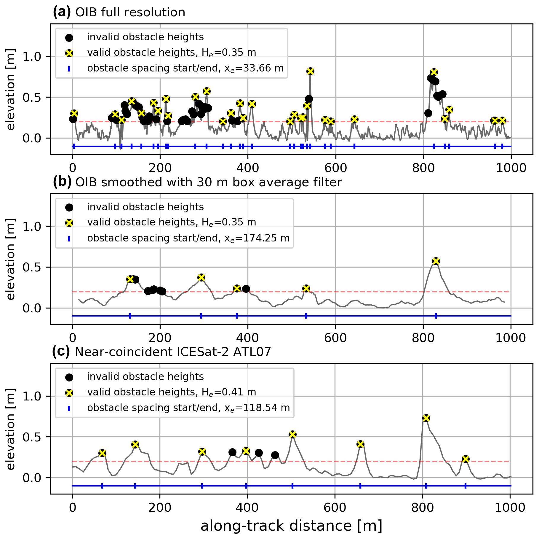
Figure 1(a) Sea ice feature statistics from a sample OIB ATM flight on 19 April 2019 (88.0∘ N, ∼ 170.7∘ E). Panel (b) is the same as (a) but smoothed to the ICESat-2 resolution via a moving average filter with box size of 30 m. (c) Sea ice feature statistics from a near-coincident ICESat-2 ATL07 track section. Black dots show all identified maxima; the yellow “x” symbols show maxima that satisfy the Rayleigh criterion, the dashed red line shows the 0.2 m threshold, the blue line with dividers shows identified obstacle spacing. All data are referenced to level ice (mode).
3.1 Drag coefficient regression with airborne lidar measurements
Taking the spring 2019 OIB/ICESat-2 underflights (4 d in 2019) that were near coincident with the measurements of ICESat-2, we can calculate drag coefficients from both datasets and compare the results. The shortest time lag during the underflight was less than 1 min for three of the flights (8, 12 and 19 April 2019) (Kwok et al., 2019a); however, 8 and 12 April are overlapping racetracks conducted for a time period of ∼ 8 h, and thus the time lag is highly variable (all legs were considered to maximize the total amount of data). The shortest time lag on 22 April, also used for this comparison, was ∼ 38 min (Kwok et al., 2019a). We used a subset of all OIB data that fell within the specified azimuthal angle range of the ATM scanner, which likely reduced the spatial coincidence as well. As a result, we did not simulate a one-to-one elevation comparison as has already been done in Kwok et al. (2019a) and Ricker et al. (2023), and thus we did not employ any drift correction. Since we look at 10 km averages for the purpose of comparing regional average form drag, it was sufficient to compare averaged data of similar ice regimes and not to focus on the coincidence itself. Since the averages are not aligned, the datasets are gridded to a 12.5 km grid, and the comparison takes place between matching filled-in grid cells (see Fig. 2).
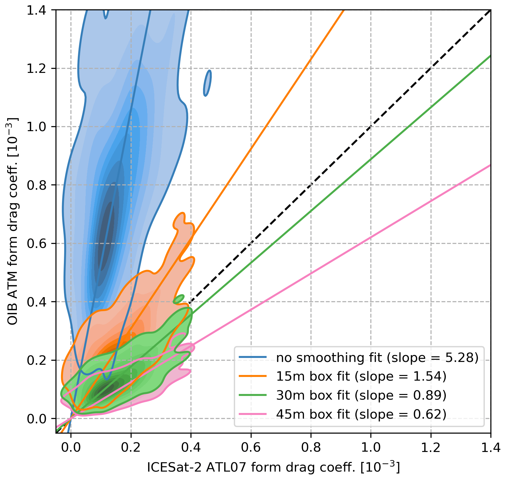
Figure 2Heat maps of 12.5 km grid resampled 10 km average ICESat-2 ATL07 form drag coefficients plotted against those computed from OIB ATM drag coefficients from 4, 8, 19 and 22 April 2019, which are resampled and calculated in the same manner. The blue heat map and line of best fit represent the base drag coefficients from ICESat-2 ATL07 and the full-resolution OIB ATM data; this regression is the basis for the scaling applied to ICESat-2 drag coefficients. The other three heat maps feature OIB ATM data smoothed by a moving average filter with window sizes of 15 m (in orange), 30 m (in green) and 45 m (in pink). The norm for each of the heat maps is different to show the full variability of each and avoid oversaturation. The lines represent Huber fits with color coding matching that of the bivariate heat maps (except for the dashed black line that represents the identity line).
Thus, Fig. 2 shows a comparison between form drag coefficients calculated from ICESat-2 ATL07 and OIB ATM segments (blue). This slope (in blue) is the scaling that is applied to the ICESat-2 ATL07 drag coefficients to amplify the retrieved signal, while the orange, green and pink lines are simply tests done to better explain the relation between the satellite and airborne datasets. As expected, the majority of form drag coefficients calculated from OIB ATM occupy a wider range (∼ 0.3–1.3 ) than their ICESat-2 ATL07 grid cell counterparts (∼ 0–0.3 ). As demonstrated in Fig. 1, we can simulate ICESat-2 ATL07 by passing all OIB ATM data through a moving average filter of varying box size (15, 30 and 45 m) and observe that we can get the line of best fit to match the one-to-one line depending on the size of the averaging box (Fig. 2). Smoothing with a box size of 30 m, which is comparable to the ATL07 strong beam ∼ 30 m spatial resolution (Kwok et al., 2019b), results in a line of best fit that is the closest match to the one to one line, which is encouraging. Box sizes of 15 and 45 m are shown for comparison's sake and are meant to demonstrate how both too little and too much of this smoothing can fail to produce values comparable to that of ICESat-2.
The beam used for model training is the second strong beam as it is in best spatial agreement with all four OIB ATM flight near-coincident datasets (Kwok et al., 2019a). Using the line of best fit from Fig. 2 (in blue), we correct the ICESat-2 ATL07 form drag coefficients towards the OIB ATM form drag coefficient range using the scaling factor 5.28. Here we focused on comparing the average drag coefficients from satellite and airborne instruments rather than the component parameters: obstacle height and obstacle spacing. The reason for this approach is because that is where the best regression was found. Regressing obstacle heights shows decent agreement, but evaluating the different box sizes on the OIB values shows very small differences. The differences are small because while the smoothing introduced in ATL07 effectively retrieves the tall narrow ridges as smaller than they really are, this also pushes a lot of small ridges below the cutoff, reducing the sample size. This reduction results in similar averaged values between the smoothed and high-resolution datasets, as can be seen in Fig. 1a and b, where the average obstacle height He is the same. The only exceptions are the features that are not detected at all (Ricker et al., 2023), which force the regression to be steeper than expected. With obstacle spacing, the smoothing gets in the way of extracting any meaningful relationship. As can be seen in Fig. 1a and b, the smoothing reduces the sample size, which is directly proportional to obstacle spacing, as fewer obstacles translate to a higher average spacing between them. It is only through evaluating Eq. (3) with the input parameters where we see a reasonable relationship. Comparing ICESat-2 ATL07 with OIB ATM form drags with varying box size smoothing applied also shows expected results (Fig. 2), further confirming to us that regressing form drags is the best approach.
The correlation found between the drag coefficients computed from the different instruments is 0.61 (blue heat map in Fig. 2), and the mean square error (MSE) between the OIB ATM drag coefficients and the ICESat-2 ATL07 coefficients with the scaling factor applied (5.28) is . Considering some ridges are not detected (Ricker et al., 2023) due to sampling issues and the lack of perfect coincidence, we do not expect perfect correlation. Moreover, we are looking at spatial averages here, where the smoothing has a very strong effect on the ridge spacing (as can be seen in Fig. 1); this is why a topography comparison where the sampling of ICESat-2 is simulated with the OIB ATM data can show better agreement, as in Kwok et al. (2019a). However, that is not our aim in this study, here we try to make the Garbrecht et al. (2002) parameterization applicable to ICESat-2 ATL07 data and correct for the sampling issues using OIB ATM. For comparison's sake, we try to simulate ICESat-2 ATL07 with OIB ATM data with the moving average filters in Fig. 2, but we chose not to simulate the elliptical footprint of ICESat-2 in detail as in Kwok et al. (2019a) and Ricker et al. (2023) for that is not needed for the monthly pan-Arctic drag coefficient product which is the end result of this study. Unsurprisingly, comparing the correlation and MSE with the OIB ATM data (in blue) to the smoothed version (30 m box, in green, which has the best agreement with the identity line), we have found a correlation of 0.72 and a MSE of (with the scaling factor 0.89 as in Fig. 2) for the latter. This better agreement is observed as here the OIB ATM data are sampled similar to how ICESat-2 ATL07 are, and making the methods identical will raise the correlation even higher, as in Kwok et al. (2019a). What we require for our study is for the drag coefficients to be calculated as in Castellani et al. (2014) and Petty et al. (2017), making use of high resolution and high sampling of the airborne datasets, and then regressing the OIB ATM values with estimates of the spatially averaged ICESat-2 drag coefficient. In this way, we aim to improve the ICESat-2 product and amplify the signal that is lower than expected due to sampling.
For an inter-comparison of the drag coefficients processed for each of the three strong beams, see Fig. A2 in Appendix A. Using the first and third strong beams we can produce a similar result despite the model being trained with the second strong beam (the most coincident beam). To incorporate the full available high-resolution dataset and minimize random sampling errors from here on we use all three strong beams for all ICESat-2 ATL07 parameter maps.
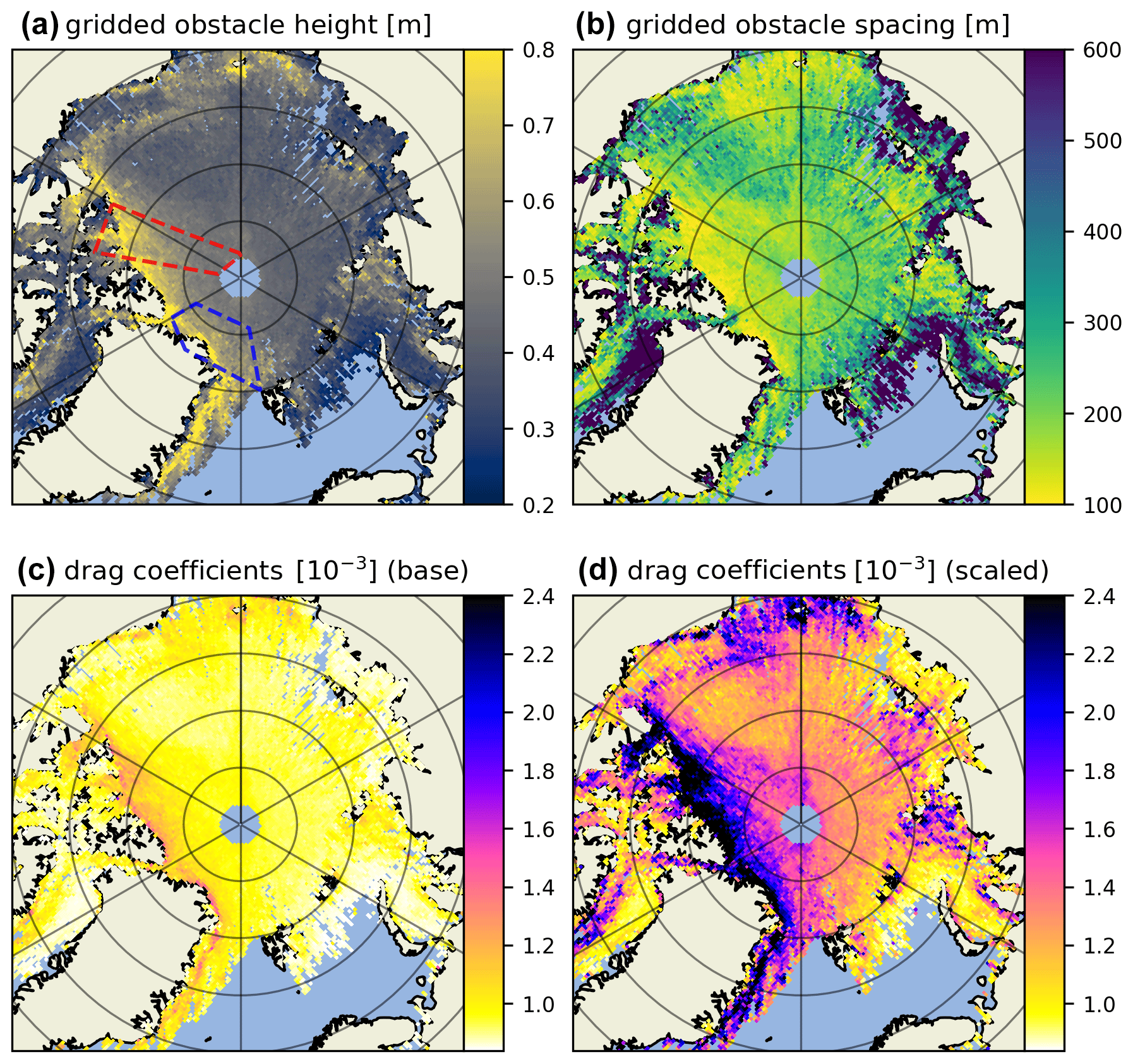
Figure 3Data computed from April 2019 ICESat-2 ATL07 tracks (all three strong beams): (a) average obstacle height, (b) average obstacle spacing, (c) total neutral 10 m atmospheric drag as computed with Eq. (3) from ICESat-2 average obstacle height and spacing. Panel (d) is the same as (c) but with the OIB ATM scaling factor (5.28) applied. In (a) zones marked in red and blue represent near-coincident OIB ATM topographic data used to generate the scaling factor via regression (8, 12, 19, 22 April 2019) and data used for evaluation (6, 20 April 2019), respectively.
In Fig. 3, we map average obstacle height and spacing used as input in Eq. (3) and the resulting obstacle form drag coefficient (), with the skin drag coefficient constant () added, for the month of April 2019. Here we do not scale with sea ice concentration (A) or consider floe edge and open-water drag components so as to focus on the difference between the scaled and base ICESat-2 ATL07 drag coefficients. The areas outlined in Fig. 3a represent the area where near-coincident OIB ATM flights took place (in red) and additional topographic data over sea ice from the month of April 2019 (6 and 20 April) that are used for the evaluation study in Sect. 3.2 (in blue). Looking just at the drag coefficients, in Fig. 3c and d we can see that with the OIB ATM scaling factor applied, the data product are in much better agreement with the pan-Arctic maps produced in Petty et al. (2017) and the regional drag assessments conducted in Castellani et al. (2014). The spatial variability across all parameters in Fig. 3 also confirms the expectation of multiyear ice that is predominantly north of Greenland and the Canadian Archipelago being more rough ( before scaling up; after) and as a consequence exhibiting a higher concentration of tall ridges (He>0.8 m) and thereby shorter spacing (xe<100 m) between them.
3.2 Evaluation study
We take advantage of OIB data from north of Greenland (outlined in blue in Fig. 3a) and collocate it to ICESat-2 ATL07 drag coefficient data produced for the month of April 2019 to perform an evaluation study of our product. In Fig. 4, we compare the drag coefficients computed from the OIB ATM dataset using the methods (see Sect. 2.3) that were used on the near-coincident “training” dataset (outlined in red in Fig. 3a) to matching grid cells from the 2019 ICESat-2 ATL07 drag coefficient map. Both the original values (Fig. 3c) in green and those multiplied by the OIB ATM scaling factor (Fig. 3d) in orange are shown along with the ones computed from the OIB ATM dataset. Notably, the distribution of the base drag coefficients is overall much narrower than the other two, with the main peak centered around ∼ and a secondary peak at ∼ . Meanwhile, the distribution of OIB ATM and scaled ICESat-2 ATL07 drag coefficients both show a similar distribution, with the main peaks centered around ∼ and smaller secondary peaks at ∼ . This suggests that our scaled ICESat-2 ATL07 drag coefficients perform reasonably well to represent the drag variability, at least for this part of the Arctic. Given that the two datasets are retrieved on different days (within the same month) with ice drifting in between, comparing them grid cell to grid cell is not meaningful as drag coefficients vary in time. If further ATM data become available from different regions in the Arctic, this evaluation should be extended.
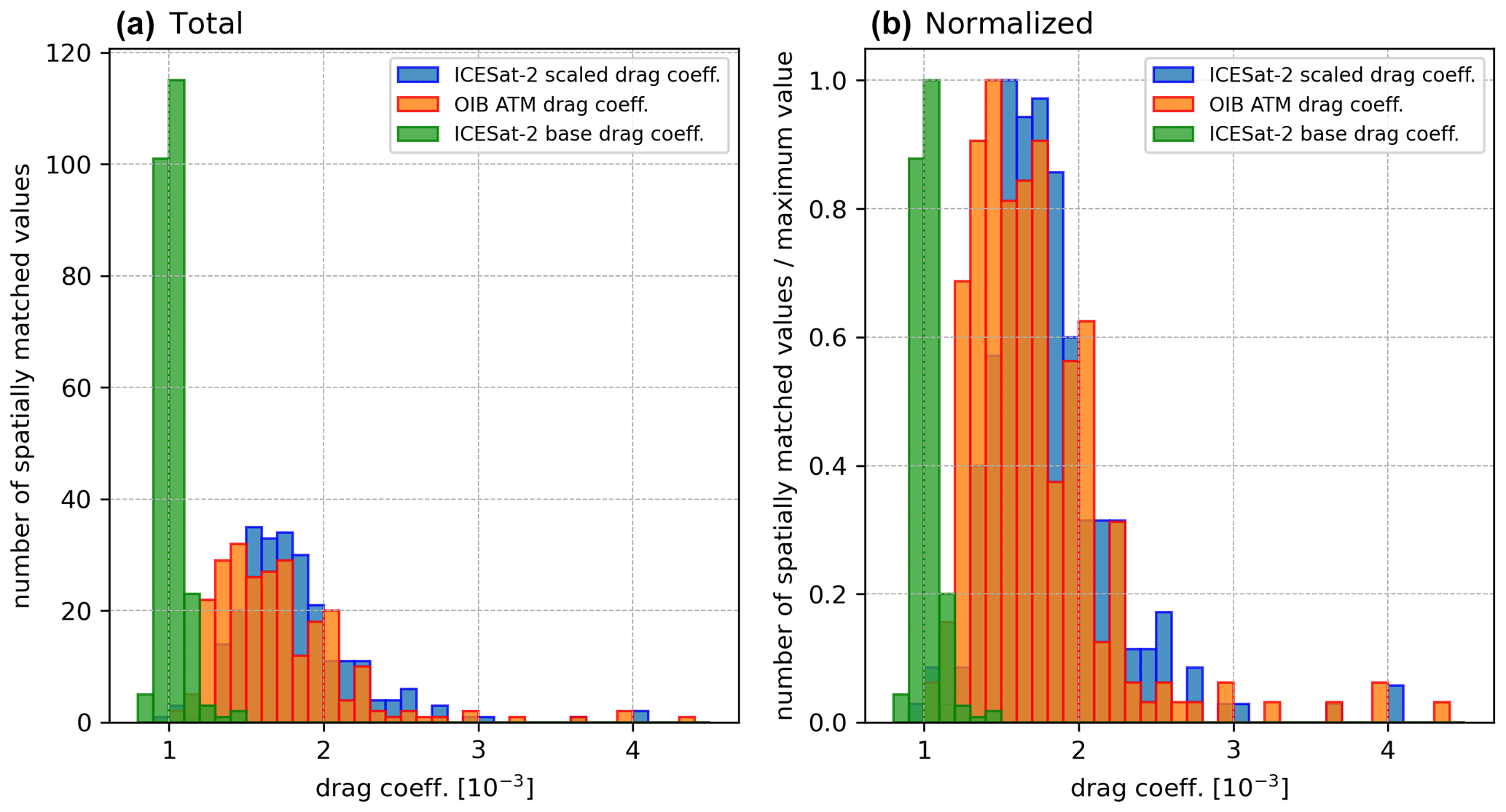
Figure 4Histograms of ICESat-2 ATL07 drag coefficients with (in blue) and without (in green) the scaling factor applied and the OIB ATM drag coefficients (in red). Here (a) shows the absolute number of matched grid cells within a given drag coefficient range, while (b) is normalized such that every value is divided by the maximum for each dataset.
3.3 Interannual drag coefficient estimates
To increase the temporal coverage of Fig. 3, we look at spatial variability in 3-month aggregates throughout 2019 in Fig. 5 (see Figs. A5 and A6 in Appendix A for the years 2020 and 2021). Here 3 months are chosen to be a reasonable time frame to maximize the data contained within individual maps on account of ICESat-2's 91 d repeat cycle (e.g., Kwok et al., 2021a, 2019b). All rows of maps within Fig. 5 contain obstacle height, spacing and drag coefficient for consecutive 3-month periods.
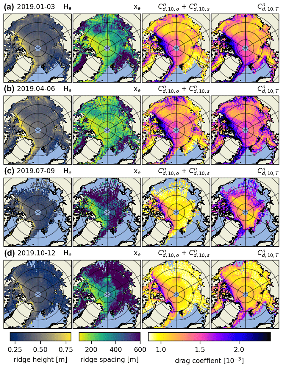
Figure 5The 2019 obstacle height (He); obstacle spacing (xe); drag coefficient as a sum of sea ice skin drag and form drag due to obstacles (); and total drag coefficient as a sum of the sea ice skin drag, form drag due to obstacles and floe edges, and open-water drag (). Importantly, the leftmost and center left columns are the obstacle heights and spacings as retrieved from ATL07, whereas in the center right and rightmost columns the form drag due to obstacles is multiplied by the OIB ATM scaling factor. The periods for which these parameters are calculated are January to March (a), April to June (b), July to September (c) and October to December (d) 2019.
In the rightmost column of Fig. 5, we include the floe edge and open-water drag coefficient terms according to Eq. (5); there we can observe drag coefficients along the marginal ice zone (MIZ). This combined parameterization is our best estimate for satellite-derived atmosphere–ice drag. It includes variable form drag due to obstacles and floe edges and constants for open-water and ice skin drag. However, drag due to floe edges next to frozen-over leads and at the edges of melt ponds in summer is not accounted for (which could be a future enhancement). By looking at the full year separated into 3-month aggregates, we can observe the spatiotemporal evolution of drag coefficients Arctic-wide. We observe a seasonal variability of up to in some multiyear ice regions, although there is a thin band of ice close to the Canadian archipelago that is consistently . Arctic-wide, this effect is comparatively smaller, but nevertheless a change of up to in total drag coefficient occurs in most areas of the Arctic. This is consistent for the years 2020 and 2021 as well (see Figs. A5 and A6 in Appendix A).
For both the center right and rightmost in Fig. 5 it is important to mention that the summer months likely exhibit higher levels of uncertainty, e.g., due to data gaps caused by clouds and due to melt ponds that can saturate the ICESat-2 photon detection system (Tilling et al., 2020). This is a consequence of melt ponds being highly specular and typically reflecting a large amount of signal photons. When ATLAS strong-beam timing channels receive more photons than they can handle within a dead time interval, they can no longer detect additional incoming photons, which can lead to short gaps in the topography data. See Tilling et al. (2020) for more information on how ICESat-2 views melt ponds.
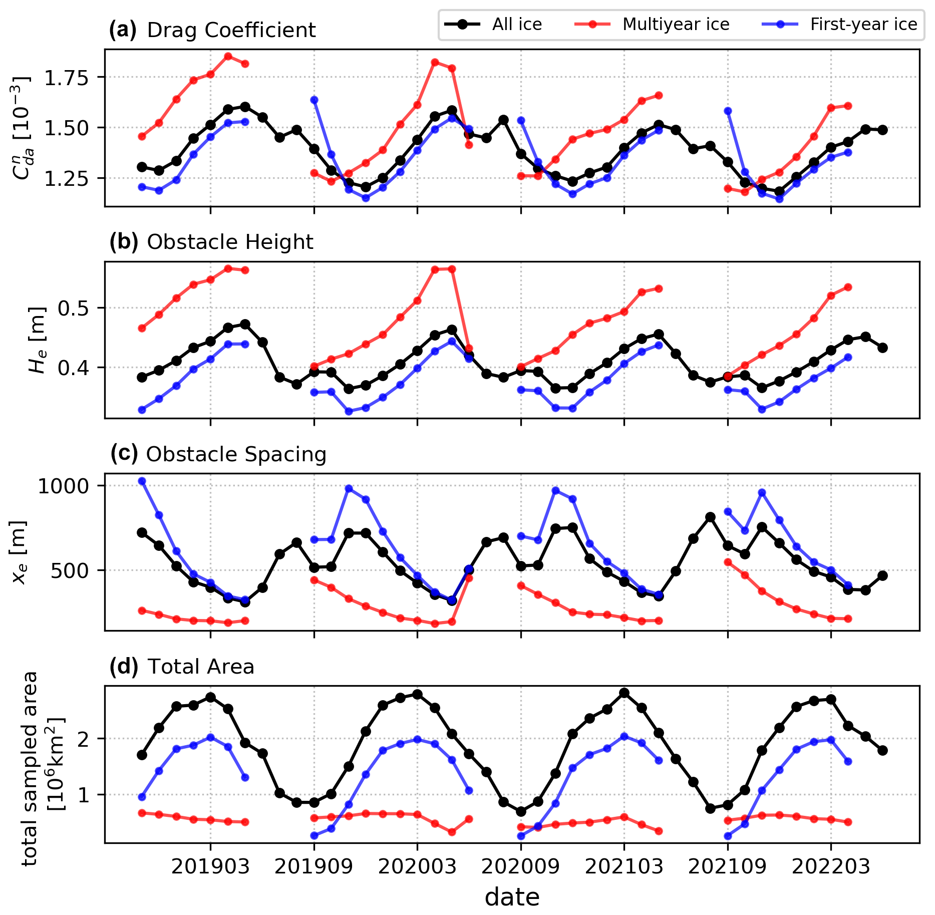
Figure 6Time series from November 2018 to June 2022 of total ICESat-2 drag coefficient (as computed in Eq. 5) with the OIB ATM scaling factor applied (a), obstacle height (b), obstacle spacing (c), and total area covered by ICESat-2 observations (d) for the whole Arctic (in black), multiyear ice (in red), and first-year ice (in blue).
To observe the seasonality as well as the monthly evolution of our best estimate of pan-Arctic total neutral drag coefficients on an interannual scale from November 2018 to June 2022, we plot the average drag coefficient, obstacle height and spacing for each month along with the total area of grid cells covered with ICESat-2 data in Fig. 6. Importantly, the total area covered is not the same as sea ice extent and is generally less than the latter due to clouds and returns with ice concentrations <15 % not being processed (Kwok et al., 2021b). Notably, both obstacle height and spacing are used to calculate the base ICESat-2 ATL07 drag coefficients; for these no corrections are applied, and thus it is expected that the heights are underestimated and the spacing overestimated as compared to OIB ATM due to smoothing by the larger ICESat-2 footprint. In addition to pan-Arctic averages, we also produce these statistics for multiyear ice (MYI) and first-year ice (FYI). Here, we make use of the MYI concentration retrieved using brightness temperatures from the microwave radiometer AMSR2 and radar backscatter from the C-band scatterometer ASCAT (Shokr et al., 2008; Ye et al., 2016a, b; Melsheimer et al., 2023). Sea ice area classified as below 50 % MYI according to the retrieval is considered FYI and used to compute FYI averages, and conversely all values equal to and above 50 % are used to compute MYI averages (see Fig. A7 for the distribution of MYI over 3-month time periods when available). By comparing the two ice types we can study the differences in their areal averages. As expected, we see higher drag coefficients (MYI: –; FYI: –) and obstacle heights (MYI: He≈0.4–0.6 m; FYI: He≈0.3–0.4 m) and conversely lower obstacle spacings (MYI: xe≈200–500 m; FYI: xe≈250–1000 m) in the averages from the MYI ice portion of the Arctic. The MYI concentration data product is only available for winter months, explaining the lack of data for the summer months in the time series. As a result this means we are unable to distinguish the FYI contribution of the form drag due to floe edges peak in August and can only estimate that upper bound given the full dataset. As for temporal evolution, there is an annual cycle in all three parameters such that the annual maximum (minimum) average drag coefficient and obstacle height (obstacle spacing) in May lags behind maximum sea ice extent, which is typically in March.
3.4 Spatial and temporal variability
Looking at our 3-monthly spatial analysis (Figs. 5, A5 and A6) and the monthly time series (Fig. 6), we corroborate the results found in Petty et al. (2017) with the MYI sea ice regions north of the Canadian Archipelago and Greenland exhibiting high drag () and the smooth FYI sea ice regions of the Beaufort (north of Alaska and western Canada), Chukchi (north of Fram Strait) and Siberian (north of Siberia) seas exhibiting low drag (). We corroborate Duncan and Farrell (2022) in terms of the distribution of spatial variability of 10 km average obstacle spacing, e.g., < 200 m near the Canadian Archipelago, for the winters of 2019, 2020, and 2022 that they have produced using the University of Maryland-Ridge Detection Algorithm. Based on the limited amount of data we analyzed, we also corroborate that the drag coefficient variability in space is larger than the variability across seasons as was found by others (Castellani et al., 2014; Tsamados et al., 2014).
We observed interesting features of ice topography, including a tongue of () sea ice that forms across the Beaufort Sea and towards a rough ice patch surrounding the Wrangel Island (near Fram Strait along the anti-meridian) only in select months (see Figs. 5b and A6b). Similarly, when Arctic sea ice extends across the Arctic Ocean and to Siberia, Severnaya Zemlya is often (but not always) surrounded by rough ice as well () (see Figs. 5b and A5b). These effects may be attributed to the movement of the Beaufort Gyre and to the tendency of ice to ridge near land. Notably, within the time span we analyzed, May is the month that repeatedly exhibits annual minimum obstacle spacing and annual maximum obstacle height and drag coefficient. This supports the notion that sea ice–atmosphere drag exhibits an annual cycle (e.g., Andreas et al., 2010). By also including drag due to floe edges, we also observe a smaller peak in August, when the ice–water boundary is at its longest. We observe a decrease in the yearly maximum average drag coefficient across all ice types during the 4 years we looked at, but given the short time frame we cannot attribute this decrease to anything more than natural variability.
3.5 Uncertainty due to sampling
While ICESat-2 has a very high resolution when compared with other laser altimeter satellites, it is still larger than the 1 m resolution of the OIB ATM data. The ATL07 segment length of about 30 m, over which 150 signal photons are obtained to lower noise in the height retrieval, smooths out the topography via the dual-Gaussian fit much like the moving average filter we applied to the OIB ATM data. This smoothing effect is discussed in detail in a recent study by Ricker et al. (2023) where coincident ICESat-2 ATL07 and airborne altimeter laser scanner (ALS) data from the MOSAiC (Multidisciplinary drifting Observatory for the Study of Arctic Climate) expedition were compared. Ricker et al. (2023) show that the ICESat-2 ATL07 strong beam could detect only 16 % of obstacles above the threshold of 0.6 m that were registered by ALS. A comparatively higher detection rate of 42 % was achieved by processing ATL03 using a higher-resolution topography dataset (Duncan and Farrell, 2022). Notably, neither of the two ICESat-2 sea ice height products were able retrieve the full extent of surface topography (Ricker et al., 2023). Assuming the lower threshold value of 0.2 m used in this study, we can expect these detection rates to rise but at some point hit a limit imposed by ICESat-2 ATL03's footprint of 11 m (Magruder et al., 2020, 2021) that is inferior to the resolution used in most modern airborne surveys looking at topography, e.g., OIB, ATM and ALS. Thus, for the purposes of our pan-Arctic study, we have chosen to stick with the publicly available and regularly updated ATL07 dataset, as either of these two data products will require some type of correction if realistic drag coefficient estimates are to be computed from them. While ATL07 has a lower obstacle detection rate locally and the obstacle height (spacing) is typically overestimated (underestimated), the spatial information on Arctic-wide obstacle distribution should be conserved according to our comparisons to airborne data (Sect. 3.1). That is why we use a regression transfer model that is trained by near-coincident OIB ATM to scale up these underestimated ICESat-2 drag values and obtain them closer to the expected form drag range estimated from higher-resolution airborne laser data.
How representative the scaling factor is for the whole of the Arctic is difficult to gauge, and with limited spatial and temporal near-coincident coverage we expect there to be some uncertainty. Despite these limitations, the racetrack OIB flights from 8 and 12 April 2019 were flown over two distinct ice types. The 8 April racetrack was 100 km north of the Sverdrup Islands (80.5∘ N) and the 12 April one was centered at 86.5∘ N in the central Arctic (Kwok et al., 2019a). As a result, the former was over thicker and rougher ice, while the latter was over thinner and smoother ice, giving us the opportunity to see how the drag coefficients compare between the two instruments in the different regimes. The scaling factors derived for the two different days are 4.42 and 5.36, respectively, resulting in an uncertainty that is in the range of ±17.5 %. This small discrepancy can also be explained by ATL07 sampling: with a smaller obstacle frequency over smooth ice, the likelihood of not detecting the few that are present increases (Ricker et al., 2023), thereby increasing the obstacle spacing used in the calculation of drag coefficients for every 10 km segment. Where the obstacle density is generally high, like in rough deformed areas near the Canadian Archipelago, there will always be an ample amount per 10 km segment to detect a higher drag coefficient signal despite the detection rate being low. Thus, the sampling issue with regard to computing drag coefficients from topography features is more prevalent over smooth ice than rough ice, and a higher correction is needed. As the 19 and 22 April OIB flights cover larger areas and the rougher deformed ice near the archipelago is rather small in extent, the scaling factor derived from all 4 d is closer to that of the 12 April racetrack and more representative of the whole Arctic, which is predominantly smoother than the ice surveyed on the 8 April.
3.6 Discussion and concluding remarks
In this study we used a combination of the Garbrecht et al. (2002) and Lüpkes et al. (2012) parameterizations to calculate obstacle drag coefficients. Although it is important to understand that this method has some uncertainty, it represents the state of the art. Currently, it is the only available parameterization of drag coefficients accounting for the effect of pressure ridges over closed sea ice cover and of floe edges in regions with fractional sea ice cover. In the following, we address the background and the uncertainties in the parameterizations, e.g., on the basis of results obtained with alternative formulations.
The parameterization idea for the effect of ridges (and other sea ice features over closed sea ice) was first tested by Garbrecht et al. (1999) on the basis of turbulence measurements made at the bow mast of RV Polarstern when the ship was drifting at different positions downstream of a large pressure ridge. Thus, this dataset was independent from the airborne turbulence data that were the main data source for Garbrecht et al. (2002). The latter dataset was validated once more in a thesis by Ropers (2013), who compared the Garbrecht et al. (2002) drag coefficients with drag coefficients derived from additional airborne turbulence and topography data. Furthermore, Castellani et al. (2014) showed that at least the average neutral 10 m drag coefficient, obtained from the Garbrecht et al. (2002) parameterization with parameters given in Sect. 2.4, agrees well with values for closed sea ice derived from Andreas et al. (2010) using SHEBA data.
It is important to understand that all available sea ice form drag parameterizations, including those for the effect of pressure ridges and of floe edges, are based on a similar formulation of dynamic pressure acting on these obstacles (Gryanik and Lüpkes, 2023). While the Lüpkes et al. (2012) approach, first formulated in a modified version by Hanssen-Bauer and Gjessing (1988), is a 2D approach, the Garbrecht et al. (2002) approach is only 1D. Ropers (2013) investigated if more complex assumptions for the latter scheme concerning the ridge geometry would improve the results, but the main conclusion was that more complex models require input variables, which are usually not available. It is furthermore important that the addition of ridge form drag to the scheme of Lüpkes et al. (2012) considered here does not represent a competing scheme. On the contrary, the formulation of Lüpkes et al. (2012) allowed the specification of the ridge component from the very beginning. Only for simplicity did they assume an average roughness of ridge-covered sea ice so that they could concentrate their work on just the edge effect. The latter was expected to be dominating in the MIZ and perhaps also in the inner Arctic under melt conditions with many leads and ponds.
The approach for floe edge form drag was also used in mesoscale modeling studies. Vihma et al. (2003) showed that the application of the scheme led to a very good agreement between modeled and observed meteorological mean variables and turbulent fluxes. Inclusion of form drag in the marginal sea ice zones using the Lüpkes et al. (2012) scheme with parameter values based on Elvidge et al. (2016) resulted in an improvement of atmospheric model results (Renfrew et al., 2019). Birnbaum and Lüpkes (2002) also investigated the effect of floe-edge-generated form drag in the marginal sea ice zone on meteorological parameters by applying a mesoscale nonhydrostatic model. They pointed to the importance of a proper choice of the coefficient of resistance cw to obtain realistic fluxes when the form drag parameterization was included. Finally, Martin et al. (2016) show that the inclusion of atmospheric form drag leads to improvements in the modeling of sea ice drift. The latter work addresses only floe edge form drag, but one can expect that further improvement is possible when ridge-generated form drag is included as well.
Thus, for the analysis of uncertainty we concentrate on the combined approach as described in Sect. 2.4. Naturally, the chosen values and formulations, e.g., for the coefficient of resistance, value of the skin drag coefficient and the inclusion of the sheltering function, contain their own uncertainties, especially when generalizing in time and space. As mentioned in Sect. 2.4, for the coefficient of resistance cw, we use an approach by Garbrecht et al. (2002) where cw depends linearly on the obstacle height He. The given coefficients in this parameterization 0.185 and 0.147 have some uncertainty because they have been derived from pressure measurements over only a few sea ice ridges. For this reason, we performed sensitivity studies with different cw formulations (e.g., Garbrecht et al., 1999; Ropers, 2013). Results are shown in Fig. A4 for April 2019 where the obstacle form drag coefficients have been calculated with the different formulations for the coefficient of resistance, taking into account necessary adjustments (modified aerodynamic roughness length and thus adjusted neutral skin drag coefficient, e.g., in the case of the Ropers (2013) version). The conducted studies showed that the principal results (geographic distribution) were unchanged, but small differences between drag coefficients are observed with the different formulations of the coefficient of resistance cw. The standard deviation (mean) was found to be (), () and () for the Garbrecht et al. (2002) formulation with the original coefficients (), the version with the natural logarithm () and the Ropers (2013) formulation (), respectively. These results are altogether not too different from the Garbrecht et al. (2002) formulation using ). The standard deviation (mean) amounts to (). Most importantly, the spatial distribution of high and low obstacle form drag regimes is conserved independent of the used cw parameterization.
Here, we tested a different hierarchy level of the Lüpkes et al. (2012) scheme than that which is used for this study (level 4). It is their level 2 parameterization which allows for specifying the measured grid-cell-averaged freeboard. Instead of the constant value 0.41 m that is implicitly used in the Lüpkes et al. (2012) version used in the previous sections, we considered the data from ATLAS/ICESat-2 L3B Daily and Monthly Gridded Sea Ice Freeboard, version 3 (ATL20), thereby implementing freeboard from satellite remote sensing measurements. Because of the smoothing imposed by sampling, the results did not show any significant improvement over using constant freeboard hf=0.41 m as recommended in Lüpkes et al. (2012) for the simpler level. Ideally, all components of floe edge form drag coefficients should be taken from remote sensing to better monitor the changing Arctic system; however, especially with regards to floe edge sizes, ICESat-2 cannot reliably determine this parameter Arctic-wide. Though it is beyond the scope of this study, we encourage future work in this direction with a multi-satellite approach that might remedy the limitations of each individual instrument. However, since in the Lüpkes et al. (2012) parameterization form drag still depends on the sea ice fraction A, the contribution of the form drag is rather small in regions with A near 1. This is the main reason why form drag is still underestimated by the level 2 scheme even when variable freeboard is allowed. This especially holds true near Greenland where ridges are tall. With respect to the application discussed here, the Lüpkes et al. (2012) floe edge form drag parameterization has uncertainties imposed by the limitations of satellite remote sensing. Namely, here we use ice concentration derived from passive microwave data (AMSR2 microwave radiometer in this case) as input, while frozen-over leads and ponds are not considered. As this freezing can already happen in August, the overall drag from floe edges is likely underestimated then. The proportionality coefficient of the Lüpkes et al. (2012) level 4 hierarchy parameterization carries with it its own uncertainty. It depends on, e.g., floe sizes and sea ice freeboard (see Lüpkes et al., 2012). Their uncertainty stems from the fact that the constant is region dependent. For this reason, sensitivity studies were carried out (not shown) in which these values were varied within realistic and recommended ranges given in Lüpkes et al. (2012) (see also Elvidge et al., 2016 and Srivastava et al., 2022). The result of this sensitivity study was that since the effect of ridge form drag was found to be much larger than the floe edge form drag, the variability in the abovementioned proportionality constant had only a small impact on the total drag coefficient.
The Garbrecht et al. (2002) approach in principle also contains the effect of sheltering by ridges. However, the sheltering function (e.g., Hanssen-Bauer and Gjessing, 1988; Lüpkes et al., 2012; Castellani et al., 2014), discussed in Sect. 2.4, was not applied to the main ICESat-2 ATL07 data after being tested to see if the data produced a non-negligible signal. By comparing the month of April 2019 (shown in Fig. 5), with and without the sheltering function implemented, the averaged absolute difference for all filled 25 km grid cells was . Thus, such a negligible difference further confirmed that the use of the sheltering function for ICESat-2 ATL07 data was not significant.
Our value for the skin drag differs from the one used in Lüpkes et al. (2012), since there the effects of ridges and other obstacles are included in the skin drag coefficient as mentioned. By using the smaller skin drag coefficient and a variable obstacle form drag coefficient (e.g., Castellani et al., 2014; Petty et al., 2017), we may introduce a more realistic obstacle form drag, since, as has been shown in this study, it varies a lot in time and space, whereas we can assume skin drag over smooth ice to be relatively constant in comparison. In the combined total drag (as derived in Eq. 5), the Garbrecht et al. (2002) obstacle form drag and Lüpkes et al. (2012) floe edge form drag parameterizations are meant to be used together to better assess pan-Arctic drag coefficients.
As mentioned previously in Sect. 1, the drag coefficient Cd also depends on the surface-roughness-dependent stability function fm, for which numerous versions exist (see, e.g., Gryanik and Lüpkes, 2018, 2023). For this study we have limited our research to assessing the neutral drag coefficients . In the case of stable stratification, Cd becomes smaller than , whereas unstable stratification with more turbulence causes Cd to be greater than (Lüpkes and Gryanik, 2015). The local near-surface stratification is heavily impacted by open water that facilitates upward heat fluxes (Andreas and Cash, 1999; Lüpkes and Gryanik, 2015) and as a result varies between the more ice-covered inner Arctic and the MIZ where open water is more common. Thus, it is in summer, where more open water is present across the Arctic ice cap, that our estimates of the neutral drag coefficients are likely below Cd. Conversely, over regions with large sea ice cover, the stratification is expected to be more stable in winter during polar nights (Lüpkes and Gryanik, 2015), which will act to offset the impact of higher form drag, suggesting our estimates of for winter are more representative of Cd.
3.7 Significance and novelty of the analysis
Using our best estimates, we have demonstrated that drag force between Arctic sea ice and the atmosphere varies annually throughout the year (see Fig. 6). The implication of this finding is that the turbulent surface flux of momentum, given in Eq. (1), also varies. In other words, depending on the month of the year, the ice is either more or less susceptible to movement depending on the amount of energy transferred to it via the atmosphere and by extension the ocean. We include the ocean here because the sources of atmospheric drag we looked at, primarily form drag due to obstacles, are closely related to the magnitude of oceanic form drag on account of pressure ridges having both a sail (the part above water) and a keel (the part below water) in roughly the same location (Timco and Burden, 1997; Tsamados et al., 2014). Similarly, form drag due to floe edges is also subject to energy transfer from the ocean for the majority of the ice edge that is below the water level. Thus both oceanic and atmospheric form drag are expected to be both temporally and spatially correlated to one another, wherein the oceanic drag is higher in magnitude (Tsamados et al., 2014). Form drag from melt pond edges, a parameter we did not look at here, we expect to be a unique component of total atmospheric drag.
We observe that MYI ice exhibits the highest drag in May (red line in Fig. 6a), due to an increase in the form drag due to obstacles, and FYI ice peaks sometime in July–August (according to the secondary peaks in the black line, i.e., all data, in Fig. 6a and the associated presumed trajectory of the blue line, i.e., FYI data) from a longer ice–water edge and the associated floe edge drag in summer months. Looking at the gridded data (Figs. 5, A5 and A6), we can further comment on developments on regional scales. Notably, it is the Lincoln Sea, north of Greenland, which exhibits the highest form drag due to obstacles with high drag coefficients (2–3× higher than smooth FYI areas, e.g., the East Siberian Sea) reaching as far north as 85∘ in the months of spring (panels a and b in each of the aforementioned figures). However this is not consistent throughout the year as these relatively high drag coefficients tend to retreat towards the Canadian archipelago throughout summer and autumn (panels c and d in each of the aforementioned figures). Interestingly, it is not consistent across all years either, as this behavior was not observed in 2021 (Fig. A6). Similarly, the neighboring Beaufort Sea and Fram Strait (mixture of MYI and FYI) also exhibit wide areas of higher form drag coefficients sometime in late spring (panel b in each of the aforementioned figures). All other Arctic seas (mostly FYI) primarily show an increase in form drag due to floe edges along the MIZ (see the rightmost column in the aforementioned figures) but also in small part higher form drag due to obstacles near land features. Thus, these data prove highly valuable in terms of identifying previously unknown spatial and temporal developments in pan-Arctic and regional drag. This analysis is the first of its kind as previous studies either assumed uniform drag across the Arctic or did not provide sub-yearly temporal information.
In terms of climate modeling, our findings show that assuming a constant drag coefficient in both space and time misrepresents the variability in momentum fluxes near the surface and thus the main forcing of sea ice drift. This misrepresentation might in turn cause many other deficiencies in air–ice interaction such as insufficient variability in the sea ice concentration. Accordingly, a suitable further development of drag parameterizations for a more realistic representation of form drag seems necessary. As for understanding Arctic sea ice, we believe these data have the potential to help with better understanding the interaction between sea ice, ocean, and atmosphere; to better predict the motion of sea ice; and to identify temporal and spatial variability in pan-Arctic drag coefficients on a monthly basis. Most importantly, this study helps us link yet another crucial sea ice parameter to remote sensing. This link, given ICESat-2 or similar future mission data are available for years to come, has the potential to help us better understand the multiannual changes in Arctic sea ice cover as the local climate warms at an unprecedented pace (e.g., Serreze and Barry, 2011; Stroeve et al., 2012).
This study makes use of measured sea ice topography to calculate atmospheric drag coefficients across the Arctic ice cap on monthly and 3-monthly temporal scales. To our knowledge, it is the first analysis of monthly pan-Arctic drag coefficient estimates of its kind. The sea ice topography is obtained from the ICESat-2 ATL07 data product at variable resolutions that depend on surface reflectivity but average around 30 m for the strong beams (Kwok et al., 2019b). Using methods developed in Garbrecht et al. (1999, 2002) according to the drag partitioning scheme proposed by Arya (1973, 1975), we obtain obstacle, i.e., ridges, height, and spacing averages for 10 km segments. We then combine the estimated form drag due to obstacles with sea ice skin drag, drag due to floe edges and a drag due to open water; all of which are incorporated as constants scaled differently with sea ice concentration.
In conclusion, from our analysis of pan-Arctic drag coefficients from the year 2019 and to a lesser extent 2018, 2020, 2021 and 2022, we have observed several noteworthy natural phenomena. Pan-Arctic form drag due to obstacles follows an annual cycle that is similar in both MYI and FYI regions. The yearly maximum average drag coefficient is not connected to the yearly maximum sea ice extent and seems to occur after the sea ice extent maximum. Form drag due to obstacles is primarily spatially variable (high in MYI regions and low in FYI regions) but nevertheless shows some temporal variability (maximum in May and minimum in December). Our results suggest that form drag due to floe edges is more prevalent during summer months when large areas are broken up and the MIZ expands, whereas form drag due to surface features peaks in late spring when its contribution is magnified from MYI regions north of the Canadian Archipelago and Greenland.
While it is beyond the scope this study, we propose the possibility of extending ICESat-2-based analysis to also estimate form drag due to floe edges from satellite measurements rather than using a constant as mentioned in Sect. 3.6. We encourage the open-water drag component to be derived from a parameterization that takes into account wind speed and therefore wave height that might cause additional form drag across water surfaces. We propose the use of lead and melt pond data to account for additional sources of drag not included in our study, e.g., lead and melt pond edges.
Using our methods, we obtain a sufficient amount of data to mostly fill a polar stereographic 25 km grid via bucket resampling for each month to produce a pan-Arctic monthly total neutral atmospheric drag coefficient analysis. On account of ICESat-2's near-polar orbit, the data density is highest around the pole hole and wanes at lower latitudes (see Fig. A1A). As a result, the regional drag coefficient estimates at higher latitudes are more representative of the time periods shown in Figs. 3, 5, A5 and A6, whereas those at lower latitudes are computed with fewer height measurements (often just a few select days). In other words, rather than a temporal mean of surface topography, it is a dataset that is sewn together with the best representation of the temporal mean near the pole hole. However, keep in mind that we do not see any discontinuities due to variable sampling in the final atmosphere–ice drag maps. In Fig. A1B one can observe the typical spacing between ATL07 height estimates, which is typically around ∼ 11–13 m but can be higher due to dark surfaces, over which up to 200 m might be needed to collect the sufficient signal photons Kwok et al. (2021a). Similarly, clouds can also increase the spacing as no measurements are retrieved beneath them.
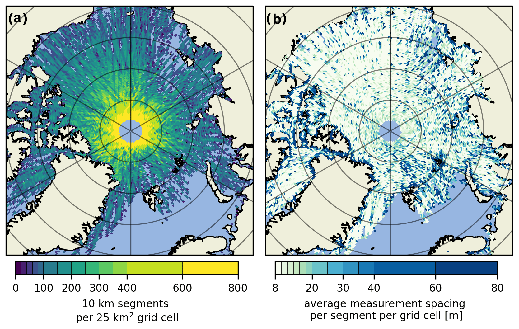
Figure A1The data distribution for the April 2019 drag coefficient map given as the number of 10 km segments from all strong beams per 25 km2 grid cell (a). The average point spacing within each 10 km segment per 25 km2 grid cell (b).
For a comparison between different beams, all of which we combine in our final data product, we refer the reader to Fig. A2. Inter-beam variability due to different range biases is present and was reported on by the ICESat-2 Project Science Office (PSO) in their preliminary analysis (e.g., Bagnardi et al., 2021). In addition, there is the 3.3 km inter-beam spacing, which suggests ridges and snow features captured by one beam might not be captured by the rest. At first glace Fig. A2d, the inter-beam standard deviation, suggests more variability in the MYI rough ice areas, but this is because the OIB ATM scaling factor applied to all data scales up all drag coefficients linearly, and hence the variability is increased in those areas as well.
Though it is not the subject of this study, we also briefly looked at the relation between the parameters extracted from ICESat-2 ATL07 which were used in Eq. (3) with respect to each other and the form drag due to obstacles derived from them. We corroborate Brenner et al. (2021), who looked at the keels instead of sails or ridges, that obstacle height and spacing indeed exhibit a negative correlation. Though not always associated with each other (Tin et al., 2003), sails and keels are predominantly spatially coincident and are therefore expected to exhibit proportional heights and depths and similar spacing. When looking at the nonlinear cutoff at 200 m for ridge spacing that can be seen in Fig. A3b and c, it is important to once again consider the “smoothing” and low obstacle detection rates (Ricker et al., 2023) of ICESat-2 ATL07 that are likely the cause of average obstacle spacing not being any lower than what is observed.
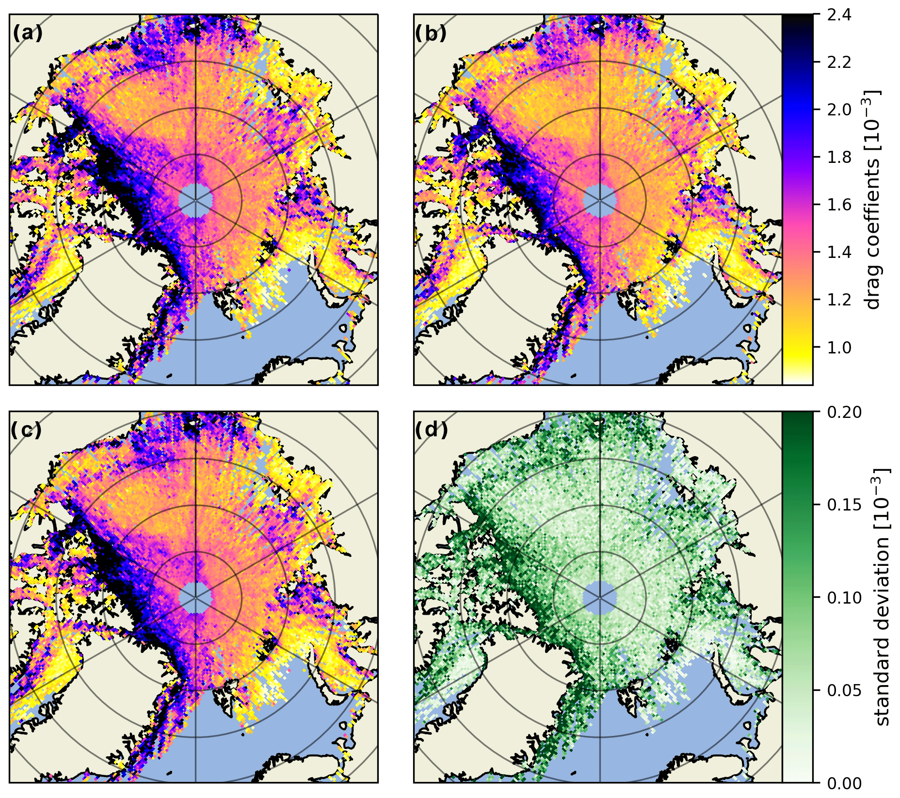
Figure A2Comparison between drag coefficient estimates (sea ice form drag plus skin drag) computed from the first (a) second (b) and third (c) strong beams and the standard deviation between them (d). All three examples have the OIB ATM scaling factor applied.
Here (Fig. A4) we also show the sensitivity studies done with different coefficient of resistance cw formulations.
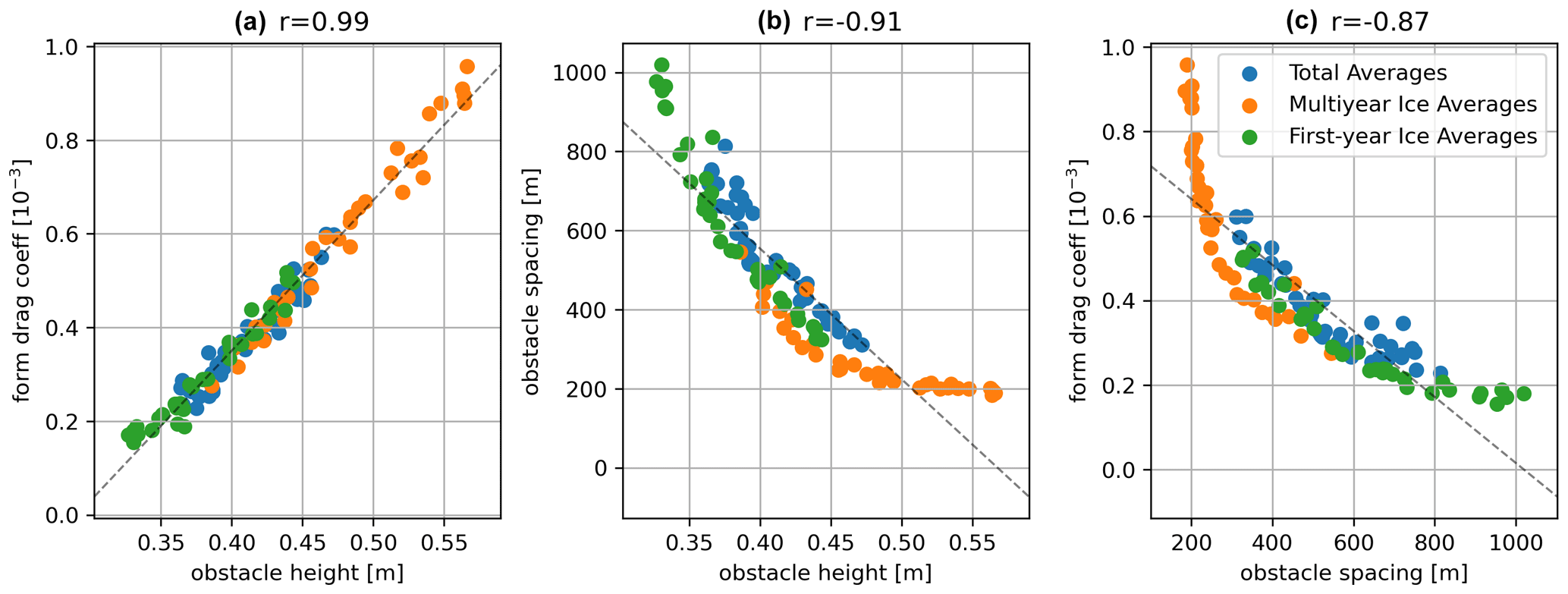
Figure A3Scatterplots between (a) obstacle height and form drag coefficient, (b) obstacle height and obstacle spacing, and (c) obstacle spacing and form drag coefficient. All values are taken from Fig. 6, such that blue dots represent the monthly pan-Arctic averages, orange dots represent monthly MYI averages and green dots represent monthly FYI averages.
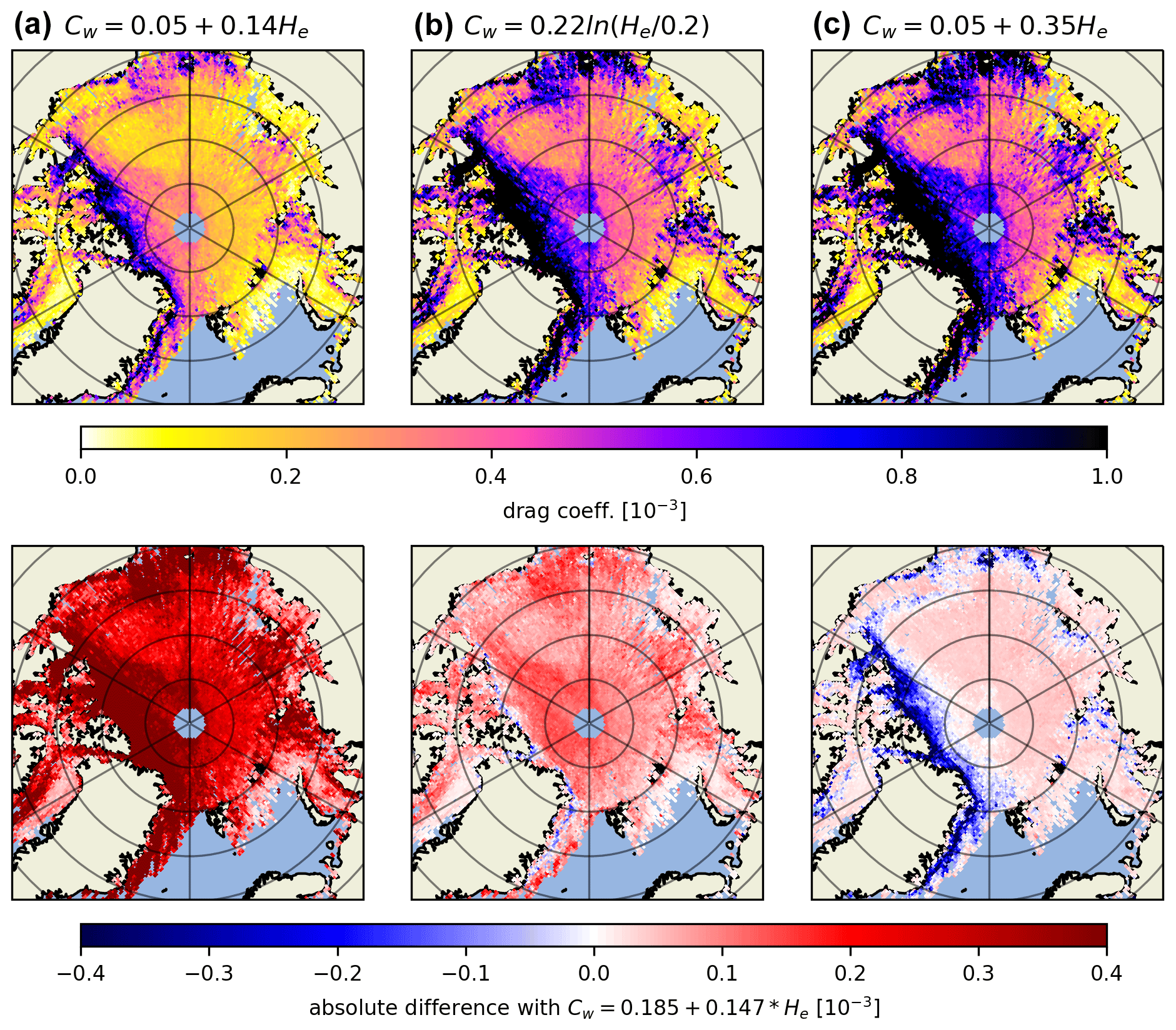
Figure A4Obstacle form drag coefficient monthly maps for April 2019 subdivided into columns labeled by the coefficient of resistance formulation used. Panel (a) uses (Banke and Smith, 1975; Garbrecht et al., 2002), panel (b) uses as suggested by Garbrecht et al. (1999) with all He values below 0.5 set to 0.2 to avoid very low and negative values, and panel (c) uses from Ropers (2013) with an adjusted aerodynamic roughness length of m. The second row shows the absolute difference between drag coefficients for each of these cw formulations as compared to the one used in this study, i.e., , with the modified coefficients from Garbrecht et al. (2002).
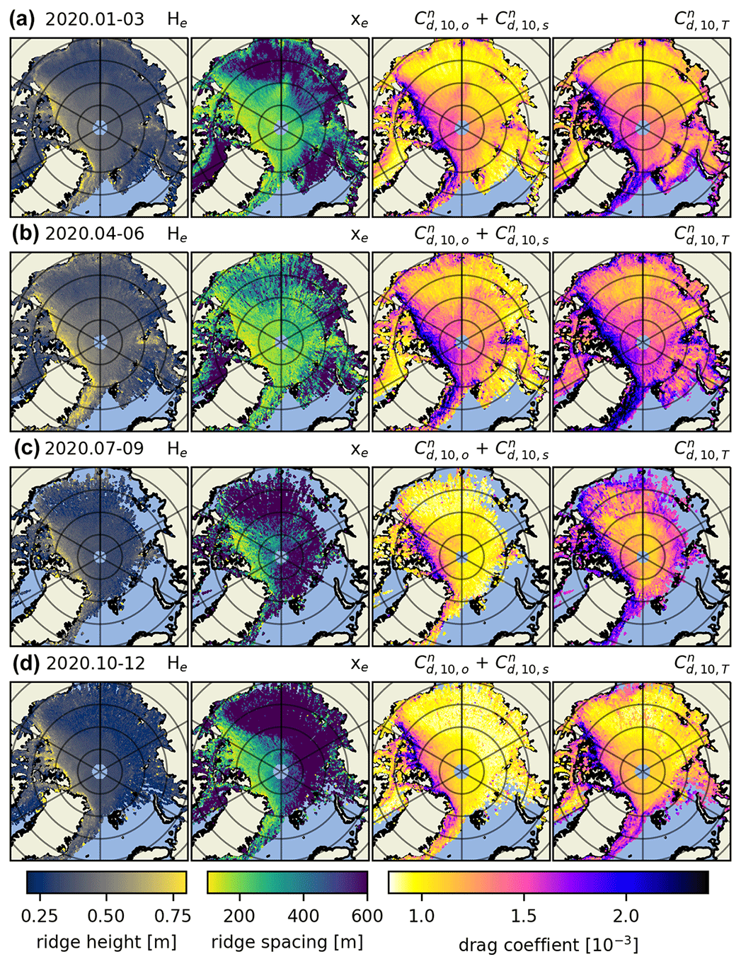
Figure A5The same as Fig. 5 but for 2020. Obstacle spacing (xe); drag coefficient as a sum of sea ice skin drag and form drag due to obstacles (); and total drag coefficient as a sum of the sea ice skin drag, form drag due to obstacles and floe edges, and open-water drag ().
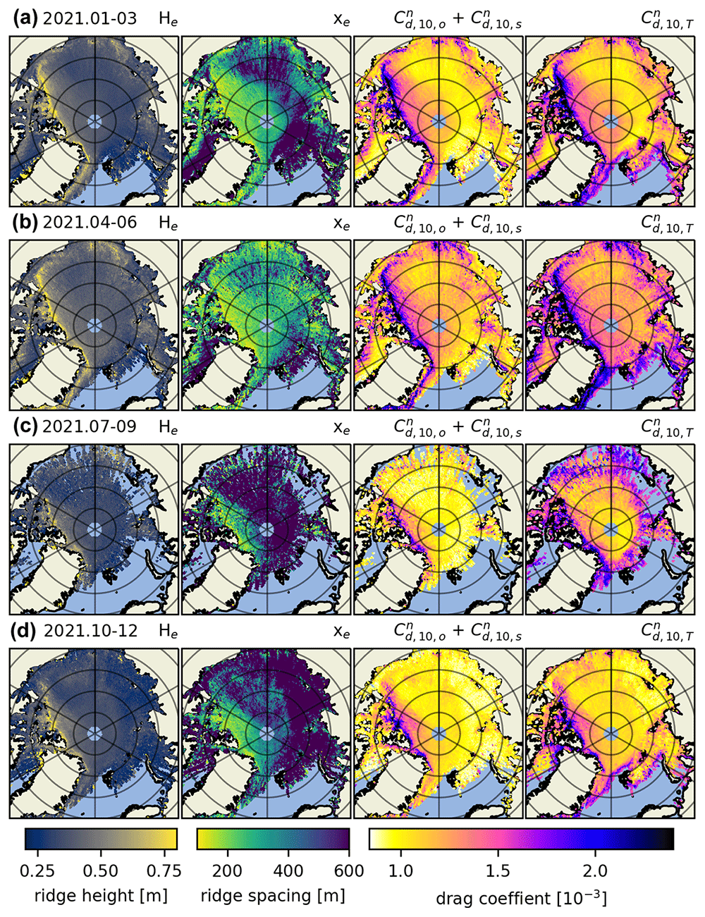
Figure A6The same as Fig. 5 but for 2021. Obstacle spacing (xe); drag coefficient as a sum of sea ice skin drag and form drag due to obstacles (); and total drag coefficient as a sum of the sea ice skin drag, form drag due to obstacles and floe edges, and open-water drag ().
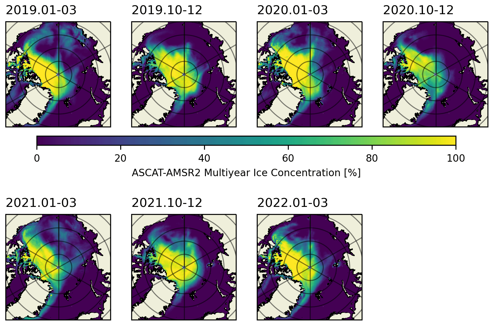
Figure A7ASCAT-AMRSR2 multiyear ice concentration winter 3-month averages for the period January 2019–March 2022.
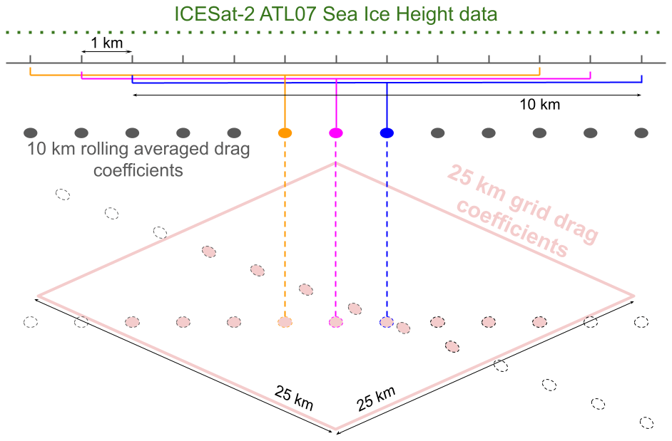
Figure A8Above is a schematic showing the data processing steps. The dotted green line indicates the ATL07 sea ice height data. The grey line shows 1 km increments, and the orange, pink and blue segments show typical 10 km windows over which the obstacle height and spacing are averaged (the drag coefficient is then calculated using these according to Eq. (3), depicted in the schematic as segments turning into dots). The resulting 10 km average drag coefficients are then gridded (e.g., the orange, pink and blue dots from the given ATL07 track are projected onto a polar stereographic grid, along with other values from the same track and those from other tracks from the same month). Finally, the values are bucket resampled to give a monthly 25 km gridded drag coefficient map (where an individual grid cell is highlighted in light red in the schematic, which is not to scale).
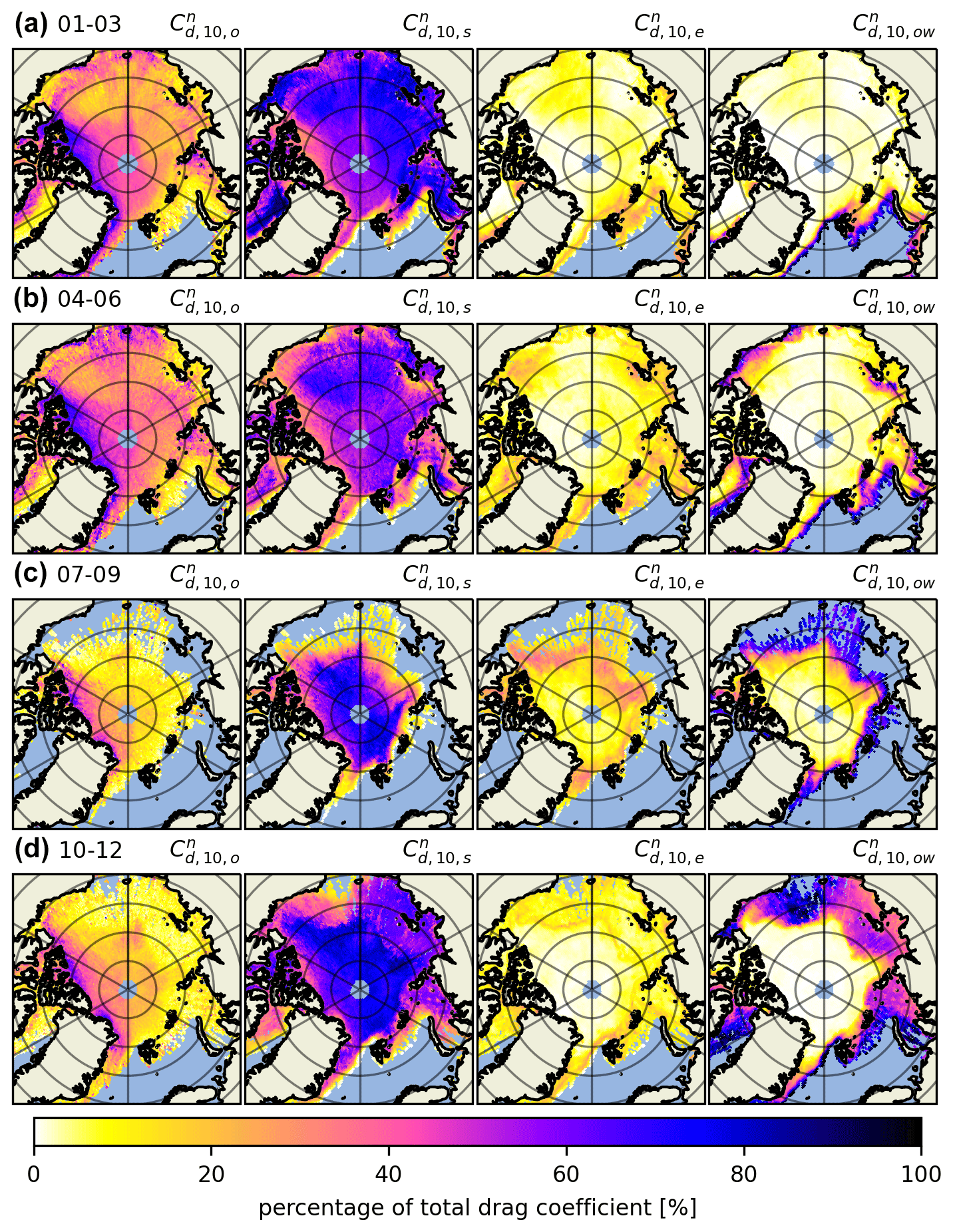
Figure A9The components of the total drag coefficient given as percentages where the columns are obstacle form drag (), sea ice skin drag (), floe edge form drag () and open-water skin drag (), respectively. These 3-monthly averages are from the year 2019 and depict the contribution of the four components of the total drag coefficient (rightmost column in Fig. 5).
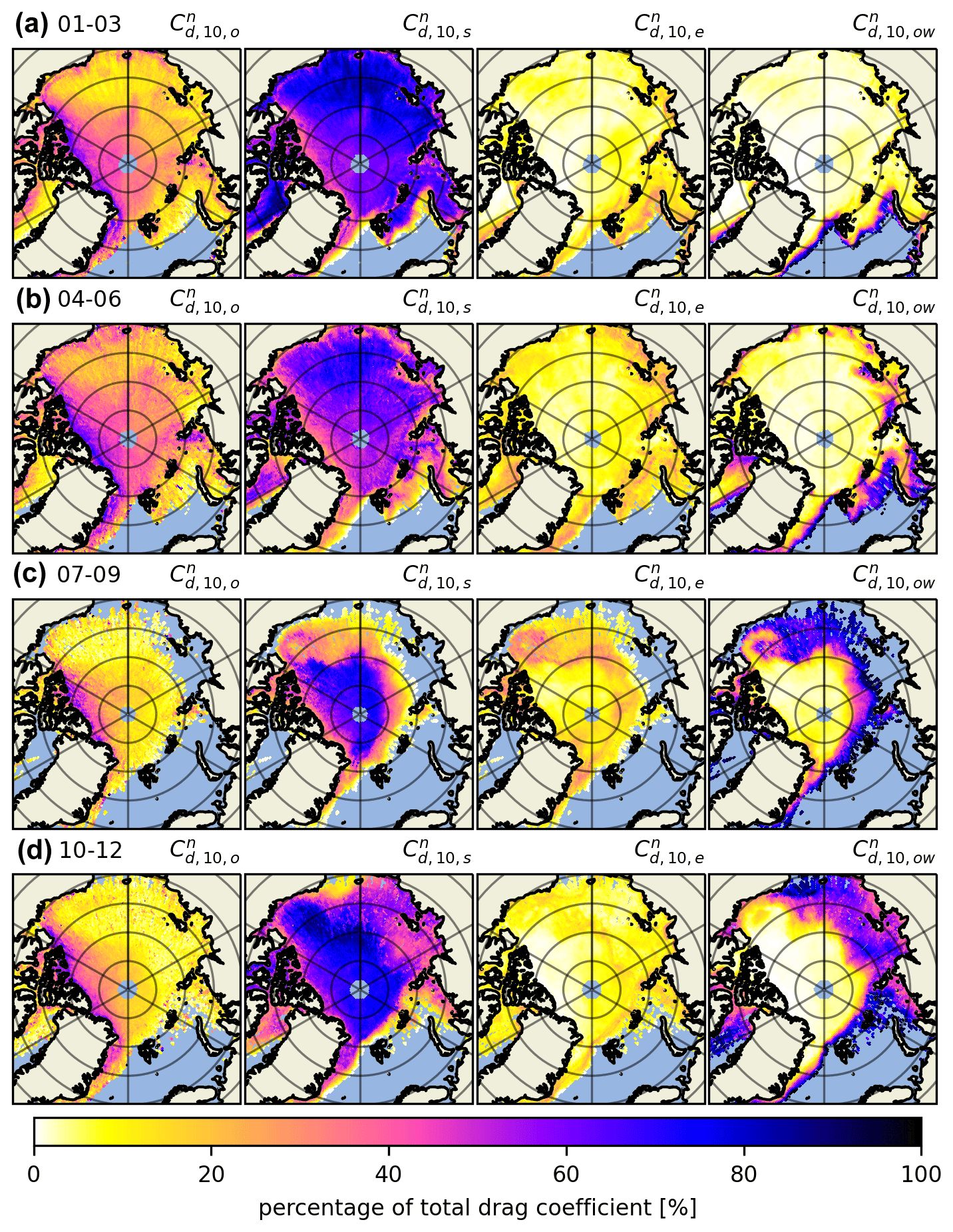
Figure A10The components of the total drag coefficient given as percentages where the columns are obstacle form drag (), sea ice skin drag (), floe edge form drag () and open-water skin drag (), respectively. These 3-monthly averages are from the year 2020 and depict the contribution of the four components of the total drag coefficient (rightmost column in Fig. A5).
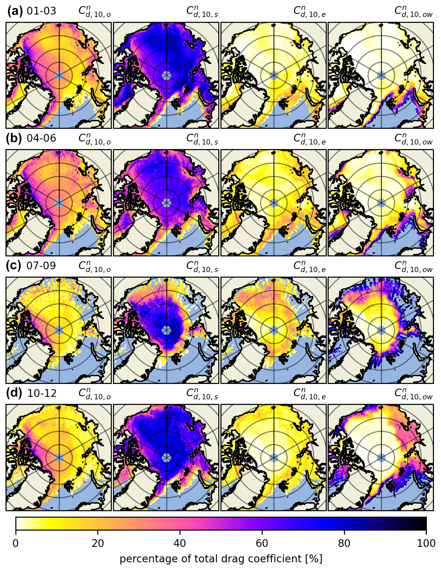
Figure A11The components of the total drag coefficient given as percentages where the columns are obstacle form drag (), sea ice skin drag (), floe edge form drag () and open-water skin drag (), respectively. These 3-monthly averages are from the year 2021 and depict the contribution of the four components of the total drag coefficient (rightmost in Fig. A6).
The AMSR2 ASI Sea Ice Algorithm sea ice concentration data product (https://doi.org/10.1594/PANGAEA.898399; Melsheimer and Spreen, 2019; Spreen et al., 2008) and AMSR2/ASCAT Multiyear ice concentration data product (Shokr et al., 2008; Ye et al., 2016a, b; Melsheimer et al., 2023) are used from local repositories and are publicly available at https://seaice.uni-bremen.de/data-archive/ (Remote Sensing for Polar Regions working group from the Remote Sensing department at the Institute of Environmental Physics, 2023).
The NASA ICESat-2 ATL07 sea ice height (version 5) data product is obtained from https://doi.org/10.5067/ATLAS/ATL07.005 (Kwok et al., 2021b). The NASA OIB ATM L1B elevation data product (version 2) is obtained from https://doi.org/10.5067/19SIM5TXKPGT (Studinger, 2013).
The processed data files used to produce the figures in this research can be found on PANGAEA (https://doi.org/10.1594/PANGAEA.959728, Mchedlishvili et al., 2022).
All authors contributed to the development of the methods used, description of relevant information, and the discussion and interpretation of the results. AM wrote most of the paper and the main algorithm for the analysis. CL provided his expertise for the parts of the paper dealing with the parameterization used and the general mathematical background behind the study. AP was conferred with for all ICESat-2-related matters, contributed to the programming behind the analysis and helped structure the paper. MT contributed to the programming and acted as supervisor during a brief research stay at University College London when this paper was in the works. GS acted as main supervisor and helped guide the development, analysis and writing stages of this study.
At least one of the (co-)authors is a member of the editorial board of The Cryosphere. The peer-review process was guided by an independent editor, and the authors also have no other competing interests to declare.
Publisher's note: Copernicus Publications remains neutral with regard to jurisdictional claims in published maps and institutional affiliations.
We thank NASA for providing ICESAt-2 and Operation IceBridge (OIB) data used in this study. We thank Marcus Huntemann, Robert Ricker, Marco Bagnardi, Giulia Castellani, Tom Johnson, Kyle Duncan and Sinead Farrell for their insightful discussions that helped in the preparation of this study.
This research was supported by the Deutsche Forschungsgemeinschaft (DFG, German Research Foundation) within the Transregional Collaborative Research Center TRR 172 “ArctiC Amplification: Climate Relevant Atmospheric and SurfaCe Processes, and Feedback Mechanisms (AC)3” (grant 268020496) and by European Union's Horizon 2020 research and innovation programme via project CRiceS (grant 101003826).
The article processing charges for this open-access publication were covered by the University of Bremen.
This paper was edited by Yevgeny Aksenov and reviewed by two anonymous referees.
Andreas, E. L. and Cash, B. A.: Convective heat transfer over wintertime leads and polynyas, J. Geophys. Res.-Oceans, 104, 25721–25734, https://doi.org/10.1029/1999JC900241, 1999. a
Andreas, E. L., Horst, T. W., Grachev, A. A., Persson, P. O. G., Fairall, C. W., Guest, P. S., and Jordan, R. E.: Parametrizing turbulent exchange over summer sea ice and the marginal ice zone, Q. J. Roy. Meteor. Soc., 136, 927–943, https://doi.org/10.1002/qj.618, 2010. a, b, c, d
Arya, S. P. S.: Contribution of form drag on pressure ridges to the air stress on Arctic ice, J. Geophys. Res., 78, 7092–7099, https://doi.org/10.1029/JC078i030p07092, 1973. a, b, c, d, e
Arya, S. P. S.: A drag partition theory for determining the large-scale roughness parameter and wind stress on the Arctic pack ice, J. Geophys. Res., 80, 3447–3454, https://doi.org/10.1029/JC080i024p03447, 1975. a, b, c, d, e, f
Bagnardi, M., Kurtz, N. T., Petty, A. A., and Kwok, R.: Sea Surface Height Anomalies of the Arctic Ocean From ICESat-2: A First Examination and Comparisons With CryoSat-2, Geophys. Res. Lett., 48, e2021GL093155, https://doi.org/10.1029/2021GL093155, 2021. a
Banke, E. and Smith, S.: Measurement of form drag on ice ridges, Aidjex Bull., 28, 21–27, 1975. a
Birnbaum, G. and Lüpkes, C.: A new parameterization of surface drag in the marginal sea ice zone, Tellus A, 54, 107–123, https://doi.org/10.3402/tellusa.v54i1.12121, 2002. a, b, c
Bourke, R. H. and Garrett, R. P.: Sea ice thickness distribution in the Arctic Ocean, Cold Reg. Sci. Technol., 13, 259–280, https://doi.org/10.1016/0165-232X(87)90007-3, 1987. a
Brenner, S., Rainville, L., Thomson, J., Cole, S., and Lee, C.: Comparing Observations and Parameterizations of Ice-Ocean Drag Through an Annual Cycle Across the Beaufort Sea, J. Geophys. Res.-Oceans, 126, e2020JC016977, https://doi.org/10.1029/2020JC016977, 2021. a, b
Castellani, G., Lüpkes, C., Hendricks, S., and Gerdes, R.: Variability of Arctic sea-ice topography and its impact on the atmospheric surface drag, J. Geophys. Res.-Oceans, 119, 6743–6762, https://doi.org/10.1002/2013JC009712, 2014. a, b, c, d, e, f, g, h, i, j, k, l, m, n, o, p, q, r, s
Dammann, D. O., Eicken, H., Mahoney, A. R., Saiet, E., Meyer, F. J., and George, J. C.: Traversing Sea Ice–Linking Surface Roughness and Ice Trafficability Through SAR Polarimetry and Interferometry, IEEE. J. Sel. Top. Appl., 11, 416–433, https://doi.org/10.1109/JSTARS.2017.2764961, 2018. a
Duncan, K. and Farrell, S. L.: Determining Variability in Arctic Sea Ice Pressure Ridge Topography with ICESat-2, Geophys. Res. Lett., 49, e2022GL100272, https://doi.org/10.1029/2022GL100272, 2022. a, b
Elvidge, A. D., Renfrew, I. A., Weiss, A. I., Brooks, I. M., Lachlan-Cope, T. A., and King, J. C.: Observations of surface momentum exchange over the marginal ice zone and recommendations for its parametrisation, Atmos. Chem. Phys., 16, 1545–1563, https://doi.org/10.5194/acp-16-1545-2016, 2016. a, b
Elvidge, A. D., Renfrew, I. A., Brooks, I. M., Srivastava, P., Yelland, M. J., and Prytherch, J.: Surface Heat and Moisture Exchange in the Marginal Ice Zone: Observations and a New Parameterization Scheme for Weather and Climate Models, J. Geophys. Res.-Atmos., 126, e2021JD034827, https://doi.org/10.1029/2021JD034827, 2021. a
Garbrecht, T., Lüpkes, C., Augstein, E., and Wamser, C.: Influence of a sea ice ridge on low-level airflow, J. Geophys. Res.-Atmos., 104, 24499–24507, https://doi.org/10.1029/1999JD900488, 1999. a, b, c, d, e
Garbrecht, T., Lüpkes, C., Hartmann, J., and Wolff, M.: Atmospheric drag coefficients over sea ice–validation of a parameterisation concept, Tellus A, 54, 205–219, https://doi.org/10.3402/tellusa.v54i2.12129, 2002. a, b, c, d, e, f, g, h, i, j, k, l, m, n, o, p, q, r, s, t, u, v, w, x, y, z, aa, ab, ac
Garratt, J. R.: The atmospheric boundary layer, Chap. 18, Cambridge University Press, p. 316, https://doi.org/10.1002/qj.49712051919, 1992. a, b
Gryanik, V. M. and Lüpkes, C.: An Efficient Non-iterative Bulk Parametrization of Surface Fluxes for Stable Atmospheric Conditions Over Polar Sea-Ice, Bound.-Lay. Meteorol., 166, 301–325, https://doi.org/10.1007/s10546-017-0302-x, 2018. a
Gryanik, V. M. and Lüpkes, C.: A Package of Momentum and Heat Transfer Coefficients for the Stable Surface Layer Extended by New Coefficients over Sea Ice, Bound.-Lay. Meteorol., 187, 41–72, https://doi.org/10.1007/s10546-022-00730-9, 2023. a
Hanssen-Bauer, I. and Gjessing, Y. T.: Observations and model calculations of aerodynamic drag on sea ice in the Fram Strait, Tellus A, 40A, 151–161, https://doi.org/10.1111/j.1600-0870.1988.tb00413.x, 1988. a, b, c, d, e
Hibler, W. D.: Characterization of Cold-Regions Terrain Using Airborne Laser Profilometry, J. Glaciol., 15, 329–347, https://doi.org/10.3189/S0022143000034468, 1975. a
Hopkins, M. A.: Four stages of pressure ridging, J. Geophys. Res.-Oceans, 103, 21883–21891, https://doi.org/10.1029/98JC01257, 1998. a
Huber, P. J. and Ronchetti, E. M.: Regression, Chap. 7, John Wiley & Sons, Ltd, p. 172, https://doi.org/10.1002/9780470434697.ch7, 2009. a
Knowles, K. W.: A Mapping and Gridding Primer: Points, Pixels, Grids, and Cells, https://nsidc.org/data/user-resources/help-center/mapping-and-gridding-primer-points-pixels-grids-and-cells (last access: 15 October 2022), 1993. a
Kwok, R., Kacimi, S., Markus, T., Kurtz, N. T., Studinger, M., Sonntag, J. G., Manizade, S. S., Boisvert, L. N., and Harbeck, J. P.: ICESat‐2 Surface Height and Sea Ice Freeboard Assessed With ATM Lidar Acquisitions From Operation IceBridge, Geophys. Res. Lett., 46, 11228–11236, https://doi.org/10.1029/2019GL084976, 2019a. a, b, c, d, e, f, g, h, i, j, k, l
Kwok, R., Markus, T., Kurtz, N. T., Petty, A. A., Neumann, T. A., Farrell, S. L., Cunningham, G. F., Hancock, D. W., Ivanoff, A., and Wimert, J. T.: Surface Height and Sea Ice Freeboard of the Arctic Ocean From ICESat-2: Characteristics and Early Results, J. Geophys. Res.-Oceans, 124, 6942–6959, https://doi.org/10.1029/2019JC015486, 2019b. a, b, c, d, e
Kwok, R., Petty, A., Bagnardi, M., Wimert, J. T., Cunningham, G. F., Hancock, D. W., Ivanoff, A., and Kurtz, N.: ICESat-2 Algorithm Theoretical Basis Document for Sea Ice Products (ATL07/ATL10), Release 005, Algorithm theoretical basis document (atbd) for sea ice products, National Aeronautics and Space Administration, Goddard Space Flight Center, Greenbelt, Maryland 20771, https://nsidc.org/sites/nsidc.org/files/technical-references/ICESat2_ATL07_ATL10_ATL20_ATL21_ATBD_r005.pdf (last access: 22 January 2023), 2021a. a, b, c, d, e, f
Kwok, R., Petty, A. A., Cunningham, G., Markus, T., Hancock, D., Ivanoff, A., Wimert, J., Bagnardi, M., Kurtz, N., and the ICESat-2 Science Team: ATLAS/ICESat-2 L3A Sea Ice Height, Version 5, NASA National Snow and Ice Data Center Distributed Active Archive Center [data set], https://doi.org/10.5067/ATLAS/ATL07.005, 2021b. a, b
Landy, J. C., Ehn, J. K., and Barber, D. G.: Albedo feedback enhanced by smoother Arctic sea ice, Geophys. Res. Lett., 42, 10714–10720, https://doi.org/10.1002/2015GL066712, 2015. a, b
Lüpkes, C. and Gryanik, V. M.: A stability-dependent parametrization of transfer coefficients for momentum and heat over polar sea ice to be used in climate models, J. Geophys. Res.-Atmos., 120, 552–581, https://doi.org/10.1002/2014JD022418, 2015. a, b, c, d, e, f, g
Lüpkes, C., Gryanik, V. M., Hartmann, J., and Andreas, E. L.: A parametrization, based on sea ice morphology, of the neutral atmospheric drag coefficients for weather prediction and climate models, J. Geophys. Res.-Atmos., 117, 205–219, https://doi.org/10.3402/tellusa.v54i2.12129, 2012. a, b, c, d, e, f, g, h, i, j, k, l, m, n, o, p, q, r, s, t, u, v, w
Lüpkes, C., Gryanik, V. M., Rösel, A., Birnbaum, G., and Kaleschke, L.: Effect of sea ice morphology during Arctic summer on atmospheric drag coefficients used in climate models, Geophys. Res. Lett., 40, 446–451, https://doi.org/10.1002/grl.50081, 2013. a
MacGregor, J. A., Boisvert, L. N., Medley, B., Petty, A. A., Harbeck, J. P., Bell, R. E., Blair, J. B., Blanchard-Wrigglesworth, E., Buckley, E. M., Christoffersen, M. S., Cochran, J. R., Csathó, B. M., De Marco, E. L., Dominguez, R. T., Fahnestock, M. A., Farrell, S. L., Gogineni, S. P., Greenbaum, J. S., Hansen, C. M., Hofton, M. A., Holt, J. W., Jezek, K. C., Koenig, L. S., Kurtz, N. T., Kwok, R., Larsen, C. F., Leuschen, C. J., Locke, C. D., Manizade, S. S., Martin, S., Neumann, T. A., Nowicki, S. M., Paden, J. D., Richter-Menge, J. A., Rignot, E. J., Rodríguez-Morales, F., Siegfried, M. R., Smith, B. E., Sonntag, J. G., Studinger, M., Tinto, K. J., Truffer, M., Wagner, T. P., Woods, J. E., Young, D. A., and Yungel, J. K.: The Scientific Legacy of NASA’s Operation IceBridge, Rev. Geophys., 59, e2020RG000712, https://doi.org/10.1029/2020RG000712, 2021. a
Magruder, L. A., Brunt, K. M., and Alonzo, M.: Early ICESat-2 on-orbit Geolocation Validation Using Ground-Based Corner Cube Retro-Reflectors, Remote Sens.-Basel, 12, 3653, https://doi.org/10.3390/rs12213653, 2020. a, b, c
Magruder, L. A., Brunt, K. M., Neumann, T., Klotz, B., and Alonzo, M.: Passive Ground-Based Optical Techniques for Monitoring the On-Orbit ICESat-2 Altimeter Geolocation and Footprint Diameter, Earth Space Sci., 8, e2020EA001414, https://doi.org/10.1029/2020EA001414, 2021. a, b
Markus, T., Neumann, T., Martino, A., Abdalati, W., Brunt, K., Csatho, B., Farrell, S., Fricker, H., Gardner, A., Harding, D., Jasinski, M., Kwok, R., Magruder, L., Lubin, D., Luthcke, S., Morison, J., Nelson, R., Neuenschwander, A., Palm, S., Popescu, S., Shum, C., Schutz, B. E., Smith, B., Yang, Y., and Zwally, J.: The Ice, Cloud, and land Elevation Satellite-2 (ICESat-2), Remote Sens. Environ., 190, 260–273, https://doi.org/10.1016/j.rse.2016.12.029, 2017. a
Martin, C. F., Krabill, W. B., Manizade, S. S., Russell, R. L., Sonntag, J. G., Swift, R. N., and Yungel, J. K.: Airborne Topographic Mapper Calibration Procedures and Accuracy Assessment, Tech. Rep. Technical Memorandum, 215891, National Aeronautics and Space Administration, Greenbelt, Maryland 20771, Goddard Space Flight Center, https://ntrs.nasa.gov/api/citations/20120008479/downloads/20120008479.pdf (last access: 10 April 2022), 2012. a
Martin, T., Tsamados, M., Schroeder, D., and Feltham, D. L.: The impact of variable sea ice roughness on changes in Arctic Ocean surface stress: A model study, J. Geophys. Res.-Oceans, 121, 1931–1952, https://doi.org/10.1002/2015JC011186, 2016. a, b
Mchedlishvili, A., Spreen, G., Lüpkes, C., Tsamados, M., and Petty, A.: Gridded pan-Arctic total neutral atmospheric 10-m drag coefficient estimates derived from ICESat-2 ATL07 sea ice height data, PANGAEA [data set], https://doi.org/10.1594/PANGAEA.959728, 2022. a
Melsheimer, C. and Spreen, G.: AMSR2 ASI sea ice concentration data, Arctic, version 5.4 (NetCDF) (July 2012–December 2019), PANGAEA [data set], https://doi.org/10.1594/PANGAEA.898399, 2019. a, b
Melsheimer, C., Spreen, G., Ye, Y., and Shokr, M.: First results of Antarctic sea ice type retrieval from active and passive microwave remote sensing data, The Cryosphere, 17, 105–126, https://doi.org/10.5194/tc-17-105-2023, 2023. a, b
Mock, S. J., Hartwell, A. D., and Hibler, W. D.: Spatial aspects of pressure ridge statistics, J. Geophys. Res., 77, 5945–5953, https://doi.org/10.1029/JC077i030p05945, 1972. a
Neumann, T. A., Martino, A. J., Markus, T., Bae, S., Bock, M. R., Brenner, A. C., Brunt, K. M., Cavanaugh, J., Fernandes, S. T., Hancock, D. W., Harbeck, K., Lee, J., Kurtz, N. T., Luers, P. J., Luthcke, S. B., Magruder, L., Pennington, T. A., Ramos-Izquierdo, L., Rebold, T., Skoog, J., and Thomas, T. C.: The Ice, Cloud, and Land Elevation Satellite – 2 mission: A global geolocated photon product derived from the Advanced Topographic Laser Altimeter System, Remote Sens. Environ., 233, 111325, https://doi.org/10.1016/j.rse.2019.111325, 2019. a
Petty, A. A., Tsamados, M. C., Kurtz, N. T., Farrell, S. L., Newman, T., Harbeck, J. P., Feltham, D. L., and Richter-Menge, J. A.: Characterizing Arctic sea ice topography using high-resolution IceBridge data, The Cryosphere, 10, 1161–1179, https://doi.org/10.5194/tc-10-1161-2016, 2016. a
Petty, A. A., Tsamados, M. C., and Kurtz, N. T.: Atmospheric form drag coefficients over Arctic sea ice using remotely sensed ice topography data, spring 2009–2015, J. Geophys. Res.-Earth., 122, 1472–1490, https://doi.org/10.1002/2017JF004209, 2017. a, b, c, d, e, f, g, h, i, j
Remote Sensing for Polar Regions working group from the Remote Sensing department at the Institute of Environmental Physics: Sea Ice Remote Sensing at the University of Bremen, https://seaice.uni-bremen.de/data-archive/, last access: 30 June 2023. a
Renfrew, I. A., Elvidge, A. D., and Edwards, J. M.: Atmospheric sensitivity to marginal-ice-zone drag: Local and global responses, Q. J. Roy. Meteor. Soc., 145, 1165–1179, https://doi.org/10.1002/qj.3486, 2019. a
Ricker, R., Fons, S., Jutila, A., Hutter, N., Duncan, K., Farrell, S. L., Kurtz, N. T., and Fredensborg Hansen, R. M.: Linking scales of sea ice surface topography: evaluation of ICESat-2 measurements with coincident helicopter laser scanning during MOSAiC, The Cryosphere, 17, 1411–1429, https://doi.org/10.5194/tc-17-1411-2023, 2023. a, b, c, d, e, f, g, h, i, j, k
Ropers, M.: Die Auswirkung variabler Meereisrauigkeit auf die atmosphaerische Grenzschicht, Phd thesis, University of Bremen, hdl:10013/epic.42983, 2013. a, b, c, d, e, f
Schneider, T., Lüpkes, C., Dorn, W., Chechin, D., Handorf, D., Khosravi, S., Gryanik, V. M., Makhotina, I., and Rinke, A.: Sensitivity to changes in the surface-layer turbulence parameterization for stable conditions in winter: A case study with a regional climate model over the Arctic, Atmos. Sci. Lett., 23, e1066, https://doi.org/10.1002/asl.1066, 2022. a
Serreze, M. C. and Barry, R. G.: Processes and impacts of Arctic amplification: A research synthesis, Global Planet. Change, 77, 85–96, https://doi.org/10.1016/j.gloplacha.2011.03.004, 2011. a
Shokr, M., Lambe, A., and Agnew, T.: A New Algorithm (ECICE) to Estimate Ice Concentration From Remote Sensing Observations: An Application to 85-GHz Passive Microwave Data, IEEE T. Geosci. Remote, 46, 4104–4121, https://doi.org/110.1109/TGRS.2008.2000624, 2008. a, b
Spreen, G., Kaleschke, L., and Heygster, G.: Sea ice remote sensing using AMSR-E 89-GHz channels, J. Geophys. Res.-Oceans, 113, C02S03, https://doi.org/10.1029/2005JC003384, 2008. a, b
Srivastava, P., Brooks, I. M., Prytherch, J., Salisbury, D. J., Elvidge, A. D., Renfrew, I. A., and Yelland, M. J.: Ship-based estimates of momentum transfer coefficient over sea ice and recommendations for its parameterization, Atmos. Chem. Phys., 22, 4763–4778, https://doi.org/10.5194/acp-22-4763-2022, 2022. a
Steele, M., Zhang, J., Rothrock, D., and Stern, H.: The force balance of sea ice in a numerical model of the Arctic Ocean, J. Geophys. Res.-Oceans, 102, 21061–21079, https://doi.org/10.1029/97JC01454, 1997. a
Steiner, N., Harder, M., and Lemke, P.: Sea-ice roughness and drag coefficients in a dynamic–thermodynamic sea-ice model for the Arctic, Tellus A, 51, 964–978, https://doi.org/10.3402/tellusa.v51i5.14505, 1999. a
Stroeve, J., Serreze, M., Holland, M., Kay, J., Malanik, J., and Barrett, A.: Atmospheric drag coefficients over sea ice–validation of a parameterisation concept, Climatic Change, 110, 1005–1027, https://doi.org/10.1007/s10584-011-0101-1, 2012. a, b
Studinger, M.: IceBridge ATM L1B Elevation and Return Strength, Version 2, National Snow and Ice Data Center [data set], https://doi.org/10.5067/19SIM5TXKPGT, 2013. a
Studinger, M.: IceBridge ATM L1B Elevation and Return Strength, Version 2, Tech. rep., National Aeronautics and Space Administration, Boulder, Colorado USA, NASA National Snow and Ice Data Center Distributed Active Archive Center [data set], https://doi.org/10.5067/19SIM5TXKPGT, 2013, updated 2020. a
Studinger, M., Manizade, S. S., Linkswiler, M. A., and Yungel, J. K.: High-resolution imaging of supraglacial hydrological features on the Greenland Ice Sheet with NASA's Airborne Topographic Mapper (ATM) instrument suite, The Cryosphere, 16, 3649–3668, https://doi.org/10.5194/tc-16-3649-2022, 2022. a, b
Thorndike, A. S. and Colony, R.: Sea ice motion in response to geostrophic winds, J. Geophys. Res.-Oceans, 87, 5845–5852, https://doi.org/10.1029/JC087iC08p05845, 1982. a
Thorndike, A. S., Rothrock, D. A., Maykut, G. A., and Colony, R.: The thickness distribution of sea ice, J. Geophys. Res., 80, 4501–4513, https://doi.org/10.1029/JC080i033p04501, 1975. a
Tilling, R., Kurtz, N. T., Bagnardi, M., Petty, A. A., and Kwok, R.: Detection of Melt Ponds on Arctic Summer Sea Ice From ICESat-2, Geophys. Res. Lett., 47, e2020GL090644, https://doi.org/10.1029/2020GL090644, 2020. a, b
Timco, G. W. and Burden, R. P.: An analysis of the shapes of sea ice ridges, Cold Reg. Sci. Technol., 25, 65–77, https://doi.org/10.1016/S0165-232X(96)00017-1, 1997. a
Tin, T., Jeffries, M. O., Lensu, M., and Tuhkuri, J.: Estimating the thickness of ridged sea ice from ship observations in the Ross Sea, Antarctic Sci., 15, 47–54, https://doi.org/10.1017/S0954102003001056, 2003. a
Tremblay, L.-B. and Mysak, L. A.: Modeling Sea Ice as a Granular Material, Including the Dilatancy Effect, J. Phys. Oceanogr., 27, 2342–2360, https://doi.org/10.1175/1520-0485(1997)027<2342:MSIAAG>2.0.CO;2, 1977. a
Tsamados, M., Feltham, D. L., Schroeder, D., Flocco, D., Farrell, S. L., Kurtz, N., Laxon, S. W., and Bacon, S.: Impact of Variable Atmospheric and Oceanic Form Drag on Simulations of Arctic Sea Ice, J. Phys. Oceanogr., 44, 1329–1353, https://doi.org/10.1175/JPO-D-13-0215.1, 2014. a, b, c, d, e, f
Tsamados, M., Feltham, D., Petty, A., Schroeder, D., and Flocco, D.: Processes controlling surface, bottom and lateral melt of Arctic sea ice in a state of the art sea ice model, Philos. T. R. Soc. A, 373, 20140167, https://doi.org/10.1098/rsta.2014.0167, 2016. a
Vihma, T., Hartmann, J., and Lüpkes, C.: A Case Study Of An On-Ice Air Flow Over The Arctic Marginal Sea-Ice Zone, Bound.-Lay. Meteorol., 107, 189–217, https://doi.org/10.1023/A:1021599601948, 2003. a
Wadhams, P. and Davy, T.: On the spacing and draft distributions for pressure ridge keels, J. Geophys. Res.-Oceans, 91, 10697–10708, https://doi.org/10.1029/JC091iC09p10697, 1986. a
Ye, Y., Heygster, G., and Shokr, M.: Improving Multiyear Ice Concentration Estimates With Reanalysis Air Temperatures, IEEE T. Geosci. Remote, 54, 2602–2614, https://doi.org/10.1109/TGRS.2015.2503884, 2016a. a, b
Ye, Y., Shokr, M., Heygster, G., and Spreen, G.: Improving Multiyear Sea Ice Concentration Estimates with Sea Ice Drift, Remote Sens.-Basel, 8, 397, https://doi.org/10.3390/rs8050397, 2016b. a, b
Yu, X., Rinke, A., Dorn, W., Spreen, G., Lüpkes, C., Sumata, H., and Gryanik, V. M.: Evaluation of Arctic sea ice drift and its dependency on near-surface wind and sea ice conditions in the coupled regional climate model HIRHAM–NAOSIM, The Cryosphere, 14, 1727–1746, https://doi.org/10.5194/tc-14-1727-2020, 2020. a, b