Deformation lines in Arctic sea ice: intersection angle distribution and mechanical properties

Despite its relevance for the Arctic climate and ecosystem, modeling sea-ice deformation, i.e., the opening, shearing, and ridging of sea ice, along linear kinematic features (LKFs) remains challenging, as the mechanical properties of sea ice are not yet fully understood. The intersection angles between LKFs provide valuable information on the internal mechanical properties, as they are linked to them. Currently, the LKFs emerging from sea-ice rheological models do not reproduce the observed LKF intersection angles, pointing to a gap in the model physics. We aim to obtain an intersection angle distribution (IAD) from observational data to serve as a reference for high-resolution sea-ice models and to infer the mechanical properties of the sea-ice cover. We use the sea-ice vorticity to discriminate between acute and obtuse LKF intersection angles within two sea-ice deformation datasets: the RADARSAT Geophysical Processor System (RGPS) and a new dataset from the Multidisciplinary drifting Observatory for the Study of Arctic Climate (MOSAiC) drift experiment. Acute angles dominate the IAD, with single peaks at ${\mathrm{48}}^{\circ }\pm \mathrm{2}$ and ${\mathrm{45}}^{\circ }\pm \mathrm{7}$. The IAD agrees well between both datasets, despite the difference in scale, time period, and geographical location. The divergence and shear rates of the LKFs also have the same distribution. The dilatancy angle (the ratio of shear and divergence) is not correlated with the intersection angle. Using the IAD, we infer two important mechanical properties of the sea ice: we found an internal angle of friction in sea ice of ${\mathit{\mu }}_{\mathrm{I}}=\mathrm{0.66}\pm \mathrm{0.02}$ and ${\mathit{\mu }}_{\mathrm{I}}=\mathrm{0.75}\pm \mathrm{0.05}$. The shape of the yield curve or the plastic potential derived from the observed IAD resembles a teardrop or a Mohr–Coulomb shape. With these new insights, sea-ice rheologies used in models can be adapted or redesigned to improve the representation of sea-ice deformation.

1 Introduction

Sea-ice deformation is a crucial process for the polar climate. It creates areas of open water that allow enhanced heat and gas exchange, and it also forms ridges that serve as a habitat for biota and provide barriers against winds and ocean currents. The deformation patterns of sea ice in the Arctic Ocean are dominated by narrow lines where deformation concentrates (Schall and van Hecke, 2010); these lines are known as linear kinematic features (LKFs), failure lines, or shear bands (Kwok, 2001). LKFs play a primary role in the mass and energy budget of the Arctic Ocean. First, the creation of thicker ice (ridges) or open water (leads), where sea-ice growth is enhanced in winter, takes place along LKFs (Stern et al., 1995; Hopkins, 1994; von Albedyll et al., 2020, 2022). Second, shear motion and sea-ice growth along LKFs influence the halocline through pycnocline upwelling and brine injection, respectively (McPhee et al., 2005; Itkin et al., 2015; Nguyen et al., 2012). Finally, despite their small total area, open leads govern the polar ocean–atmosphere heat and moisture exchange (Maykut, 1978; Untersteiner, 1961; Tetzlaff et al., 2015). Thus, LKFs are an essential component of the Arctic climate system and need to be accurately represented in regional models for reliable regional weather predictions, navigation charts, and services to Arctic communities.

LKFs emerge from the mechanical properties of sea ice. Sea ice is often described as a granular material (Overland et al., 1998; Tremblay and Mysak, 1997; Feltham, 2005) that exhibits brittle properties (Schulson, 2002; Dansereau et al., 2016). Important mechanical properties of sea ice are imprinted in the orientation of the failure lines relative to the stress direction. More specifically, two mechanical parameters are known to play a role in the orientation of the failure lines relative to the stress direction in granular materials (Vermeer, 1990): (1) the material's strength threshold to internal stress leading to deformation, especially the ratio of shear strength to compression strength, named the internal angle of friction (Coulomb, 1773), and (2) the dilatancy, or motion perpendicular to the slip line under which the ice undergoes plastic deformation (Roscoe, 1970). While the sea-ice motion (parameter 2) can be observed via satellite remote sensing, the internal stress magnitude and direction (parameter 1) cannot be observed via satellite remote sensing at the Arctic scale. Therefore, it is impossible to measure the orientation of the LKFs with respect to the stress direction directly. To overcome these shortcomings and still retrieve the mechanical properties from the orientation of the failure lines, the vorticity at the intersections of LKFs can be used instead. By describing the rotation of ice during deformation, vorticity can be utilized to infer the main stress direction and eventually link it to the intersection angles of the LKFs (Hutter et al., 2022).

Previous studies on LKF intersection angles report single intersection angles based on small sample sizes across large spatial scales (100 m–100 km), for example, 28^∘ (Marko and Thomson, 1977), $\mathrm{30}\pm {\mathrm{4}}^{\circ }$ (Erlingsson, 1988), 30^∘ (Walter and Overland, 1993), and 34–36^∘ (Cunningham et al., 1994). From the RADARSAT Geophysical Processor System (RGPS) sea-ice motion dataset (Kwok et al., 1998), sea-ice deformation data were obtained over the Arctic Ocean with a period of 3 d, allowing the automated extraction of LKF locations and angles (Hutter et al., 2019a; Linow and Dierking, 2017). Recent work based on an LKF tracking algorithm has reported an intersection angle distribution (IAD) of between 0^∘and 90^∘with a peak between 40 and 50^∘ (Hutter and Losch, 2020). Multi-scale directional analysis on the RGPS dataset also shows that small intersection angles are dominant (Mohammadi-Aragh et al., 2020).

None of the current sea-ice models can reproduce the observed distribution of LKF intersection angles (Hutter et al., 2022). LKFs in sea-ice models emerge from the rheological model, especially from the threshold of sea-ice mechanical properties. This threshold creates LKFs because it includes a change in mechanical properties between large deformations, in the LKFs, and small deformations, in between the LKFs, i.e., the viscosity maximum for viscous–plastic (VP) models (Hutchings et al., 2005) and the damage for brittle models (Dansereau et al., 2016). This hints that the current implementations of sea-ice rheological models are not accurate enough to describe the mechanical properties of sea ice. Most climate models today simulate sea ice as a VP medium with an elliptical yield curve and normal flow rule (Hibler, 1979; Stroeve et al., 2014; Keen et al., 2021). Diffuse small deformations are represented by viscous behavior, whereas the large deformations along LKFs are represented by plastic behavior (Hutchings et al., 2005). High-resolution sea-ice VP models can represent LKFs at scales 5–7 times larger than their horizontal grid spacing (Hutter et al., 2018; Bouchat et al., 2022; Hutter et al., 2022). In the VP rheology framework, the intersection angle of LKFs depends on the parameters that define the constitutive equation: the yield curve that defines the stress at failure and the plastic potential that defines the post-failure deformation, called the flow rule (Ringeisen et al., 2021, 2019). Thus, observations of LKF intersection angles can be used to constrain those parameters. Erlingsson (1991) proposed an internal angle of friction of $\mathit{\varphi }={\mathrm{15}}^{\circ }\pm {\mathrm{2}}^{\circ }$ based on their observations of LKF intersection angles, whereas Marko and Thomson (1977) proposed $\mathit{\varphi }\simeq {\mathrm{62}}^{\circ }$. Using a small set of LKF intersection angles and the assumption that the major principal direction of the sea-ice internal stress is perpendicular to the wind direction, Wang (2007) proposed the curved diamond yield curve. However, there seems to be a need for improvement. LKF-tracking algorithms show that the current VP models overestimate the intersection angles, with an IAD peaking at 90^∘ (Hutter et al., 2019a; Hutter and Losch, 2020). This behavior is shared by all other rheological models, as revealed by a recent comparison of state-of-the-art models (Hutter et al., 2022), and is also observed using multi-scale directional analysis (Mohammadi-Aragh et al., 2020). To improve the IAD in high-resolution sea-ice models, the presented IAD could be used to improve the definition of weakly constrained sea-ice rheological parameters: the yield curve and the plastic potential.

Studying the intersection angles can provide important insights into two key questions. First, is there a relationship between intersection angles and the divergence (opening or ridging) along the LKF? In other words, does the hypothesis of the normal flow rule (Ringeisen et al., 2019, 2021), as it is currently used in sea-ice VP models, hold? Second, does the observed IAD allows us to deduce the mechanical properties of sea ice and thereby constrain the shape of the yield curve or the plastic potential? To answer these questions, we see the need to revisit the IAD as it is presented in the literature. First, the angles reported in previous studies are given in the interval between 0 and 90^∘, without defining if these angles are acute (between 0 and 90^∘) or obtuse (between 90 and 180^∘) compared with the principal stress direction. Both cases need to be separated, as they are linked to different slopes of the yield curve/plastic potential and, hence, to different shapes of the yield curve/plastic potential (Ringeisen et al., 2019). Second, following the approach of Hutter et al. (2022), we consider only conjugate pairs of LKFs, i.e., intersecting LKFs that formed simultaneously under compressive forcing.

In this paper, we use satellite-derived sea-ice drift and deformation to address the gaps outlined above. Deformation concentrates along the LKFs, and vorticity identifies the LKFs formed under compressive force. Tracking of the LKFs allows for the identification of those that formed simultaneously. Therefore, we can distinguish between conjugate and non-conjugate intersection angles and discriminate between conjugate obtuse and acute intersection angles. We apply this method to the RGPS dataset and new high-resolution deformation data surrounding the 2019–2020 Multidisciplinary drifting Observatory for the Study of Arctic Climate (MOSAiC) expedition. Both datasets have different temporal and spatial coverage and resolution; thus, they indicate if intersection angles vary in the ice cover depending on the spatial scale and geographical location in the Arctic. We aim to obtain an IAD as a reference for high-resolution sea-ice models and to infer the mechanical properties of the sea-ice cover, e.g., the yield condition and/or the plastic potential.

The remainder of this paper is structured as follows: Sect. 2 presents the different datasets used in this study (Sect. 2.1) and the algorithm for the measurements of the angles between 0 and 180^∘ (Sect. 2.2); Sect. 3 presents the results of the intersection angles for the different datasets, the divergence along LKFs, seasonal variations, estimations of internal angles of friction, and an estimation of the shape of a yield curve for sea-ice modeling; and the discussion and conclusions follow in Sects. 4 and 5, respectively.

2 Methods and data

2.1 Datasets

In this study, we will use two satellite-based sea-ice drift datasets from which sea-ice deformation is derived. Thanks to the synthetic aperture radar (SAR) data from which the drift is calculated, the datasets are available independent of weather conditions and during the polar night. The high spatial resolution (1.4 km for MOSAiC and 12.5 km for RGPS) of the deformation datasets enables us to identify individual LKFs.

2.1.1 RADARSAT Geophysical Processor System

RGPS is a widely used drift and deformation dataset based on RADARSAT SAR images (Kwok et al., 1998). The dataset covers the Amerasian Basin of the Arctic Ocean (Fig. 1) for 12 winters from 1996 to 2008. Sea-ice drift is derived by tracking points that are spaced 10 km apart in SAR images. Deformation rates are computed from these Lagrangian drift paths and are interpolated to a regular 12.5 km grid. Hutter et al. (2019a) applied detection and tracking algorithms to the regular gridded dataset and extracted deformation features, which are publicly available (Hutter et al., 2019b) and are analyzed more closely in this study.

2.1.2 Sentinel (MOSAiC)

In addition, we compute ice drift and deformation based on Sentinel-1 SAR scenes (von Albedyll and Hutter, 2023). We base this dataset on horizontal–horizontal (HH)-polarized scenes with a spatial resolution of 50 m. The scenes are located along the drift of the MOSAiC expedition (Nicolaus et al., 2022) from 5 October 2019 to 14 July 2020 except for the period between 14 January and 15 March, during which the ship was north of the satellite coverage (Fig. 1). Typically, the time between two scenes was 1 d, with a few exceptions of 2–3 d, and the size of the scenes was on average 200 km × 200 km. We compute ice drift fields based on a pattern-matching ice-tracking algorithm introduced by Thomas et al. (2008, 2011) with substantial modifications by Hollands and Dierking (2011). We retrieve divergence, shear, total deformation, and vorticity from the regularly gridded sea-ice drift output at 1.4 km resolution following the approach described in von Albedyll et al. (2020) and Krumpen et al. (2021b).

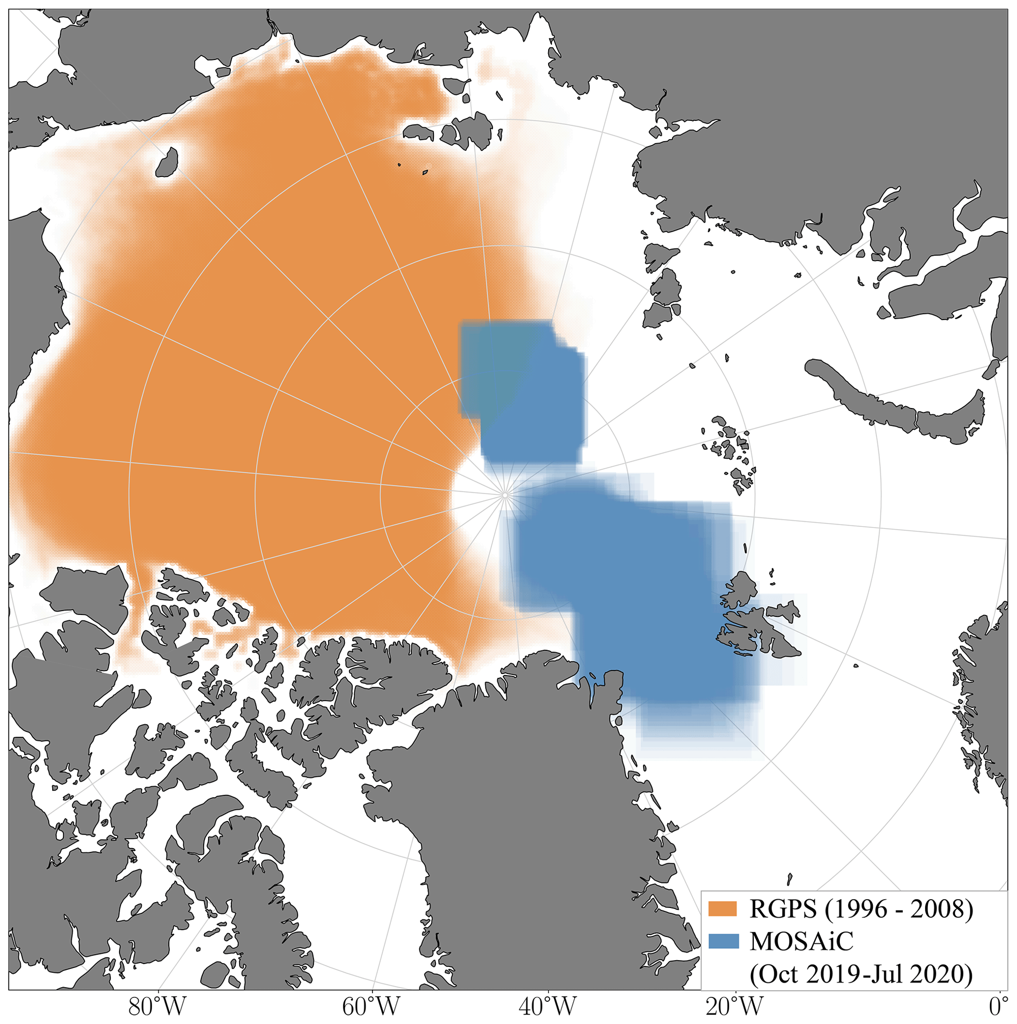
Figure 1 Coverage of the RGPS and MOSAiC LKF datasets. For the RGPS dataset, the transparency indicates the relative frequency of the coverage in the respective geographical regions.

2.2 LKF detection and angle measurement

2.2.1 LKF detection

We use the algorithms presented in Hutter et al. (2019a) to detect and track LKFs in both deformation datasets. Here, we provide a short summary of the algorithms and direct interested reader to the details in Hutter et al. (2019a). LKFs are detected in four steps: (1) pixels are marked as LKF if their deformation rates exceed the average deformation rate of the neighboring pixels, (2) all LKFs in the binary mask of LKF pixels are reduced to their skeleton using morphological thinning, (3) the binary map is divided into the smallest possible LKF segments, and (4) segments are reconnected to one LKF based on the probability of them belonging to the same LKF that is computed from their distance, orientation, and deformation rate magnitude differences. Next, the drift data are used to advect LKFs and track them over time. Note that, to exclude a direct influence of the coast, those regions are excluded from the RGPS dataset, whereas the MOSAiC dataset only covers pack ice (see Fig. 1).

For RGPS, we use the publicly available deformation data (Hutter et al., 2019b) employing the original version of the code (Hutter, 2019). For the higher-resolution MOSAiC data, we add two modifications to the original version of the detection code. First, we apply a directional filter to the input deformation rates to reduce grid-scale noise. The directional filter is a 1-D kernel spanning seven pixels that is rotated at each pixel over all directions to compute the variability along different directions. We choose the direction of lowest variability to apply the 1-D filter and compute the filtered deformation rates. This allows us to reduce noise but still preserve the linear structure of LKFs in the deformation data. Second, the morphological thinning routine was modified to align the LKF skeletons in the binary maps to the position of the highest deformation rates across the LKF. The details of both modifications can be found in the routines in dir_filter.py in the newly released version of the code (Hutter, 2023). The resulting Sentinel-1 LKF dataset is released in open-access (Hutter and von Albedyll, 2023).

2.2.2 Angle measurements

In both LKF datasets, pairs of LKF that intersect and are formed within the same time step are extracted, and the angle of intersection is measured following the approach of Hutter et al. (2019a) and Hutter et al. (2022). The angles are measured from points ca. 10 points away (in both directions) from the intersection point in order to avoid the effects of discrete orientations on a grid. In practice, because some LKFs are shorter, the number varies from 7 to 21 points. The number of 10 points was chosen to be a good compromise to get an accurate result and avoid discrete effects.

To differentiate between intersection angles that are acute ($<{\mathrm{90}}^{\circ }$) or obtuse ($>{\mathrm{90}}^{\circ }$), we use the vorticity $\left({\dot{\mathit{ϵ}}}_{\mathrm{vort}}=\frac{\mathrm{1}}{\mathrm{2}}\left(\frac{\partial u_{\mathrm{1}}}{\partial x_{\mathrm{2}}}-\frac{\partial u_{\mathrm{2}}}{\partial x_{\mathrm{1}}}\right)\right)$ along the LKFs, as shown in Fig. 2. From the vorticity information, we separate the dataset into two categories: the conjugate angles (acute and obtuse together) and the non-conjugate angles. For conjugate angles, the principal stress direction can be identified from the resulting ice motion. The ice flows from the most compressive to the least compressive principal stress. Note that, by convention, as compression is negative, the first principal stress direction is the direction with the lower compressive stress, while the second is the higher compressive stress. We do not consider the exact stresses here but rather only the principal stresses and their direction; therefore, this also includes bidirectional compression situations. The motion becomes obvious from the opposite sign of the vorticity along the intersecting LKFs (Fig. 2). In other words, for a conjugate pair of LKFs, the vorticity alternates between positive and negative along the segments of the two intersecting LKFs. For equal-sign vorticity along both LKFs, the ice motion field does not allow for the identification of the main stress direction, and we classify the intersecting pair as non-conjugate.

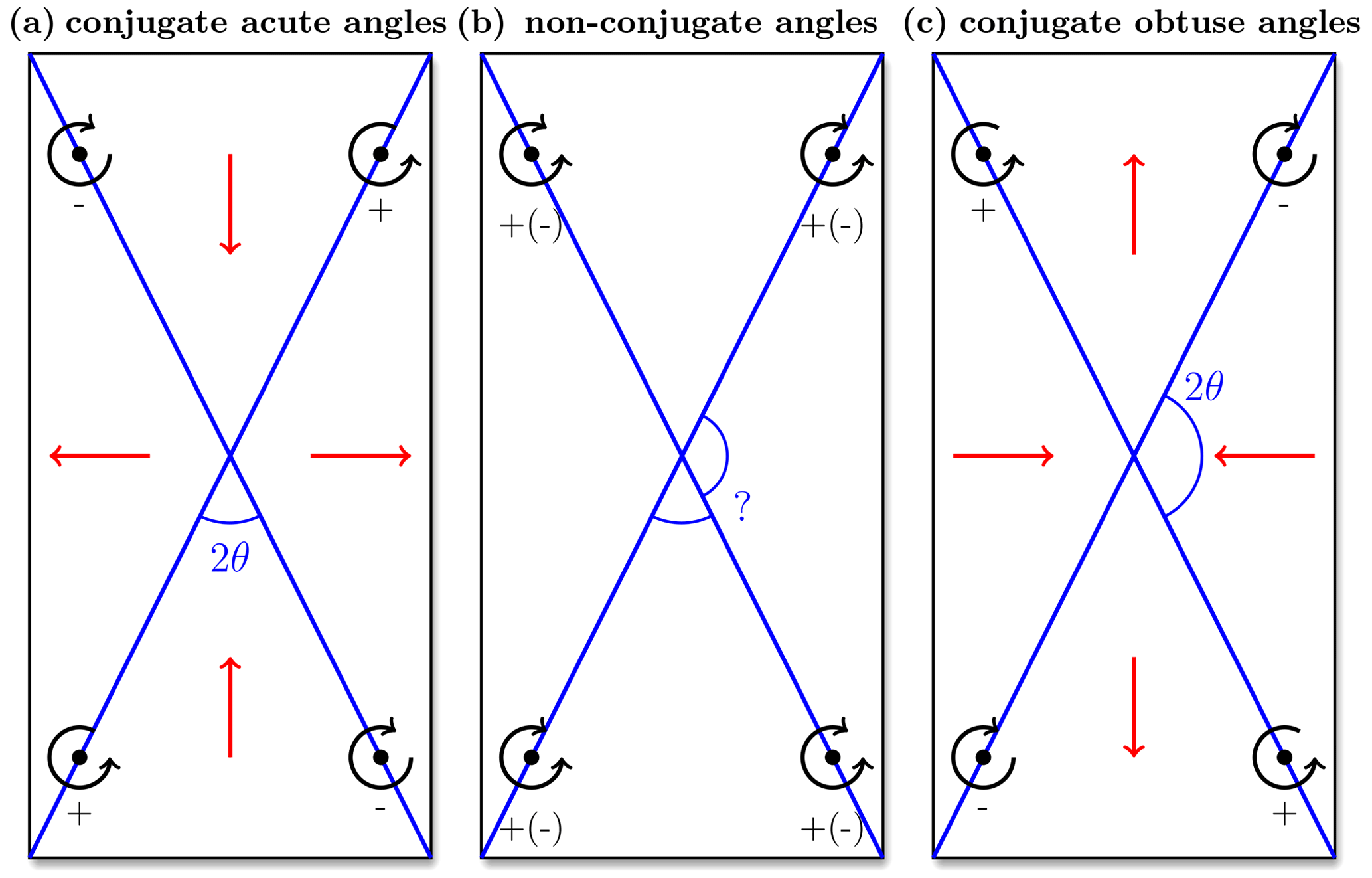
Figure 2 Schematics showing the difference between conjugate failure lines with acute and obtuse angles and those with non-conjugate failure lines. The vorticity of the ice motion (black circles with $+/-$ signs) indicates the direction of the principal stresses (red arrows), thereby differentiating between conjugate (a, c) and non-conjugate (b) failure lines.

While the generation of conjugate faults is explained by the failure of ice under compressive loading, the reasons for the existence of non-conjugate failure are less obvious. We show the distribution of the non-conjugate angles and explore reasons for these non-conjugate faults in Appendix A.

3 Results

In the following sections, we present the results of our investigation of intersection angles in both the MOSAiC and RGPS datasets. We compare the intersection angle distribution (IAD), the relationship between angles and dilatancy, and how these distributions inform us about sea-ice dynamics, especially the internal angle of friction, and the possible shape of the yield curve or the plastic potential for sea-ice VP models.

3.1 Examples of LKF intersections

Figure 3 presents three examples of LKF intersections from the MOSAiC dataset: one conjugate acute angle (Fig. 3a), one conjugate obtuse angle (Fig. 3c), and one non-conjugate angle (Fig. 3b). Especially for conjugate acute angles, we observe that LKFs with the same orientation have vorticities of the same sign (Fig. 3a). These patterns agree with the concept of fracture in diamond shapes, as shown in discrete element model (DEM) simulation (Wilchinsky et al., 2010; Heorton et al., 2018) and in theoretical works (Pritchard, 1988). For the non-conjugate and the obtuse angles, the fracturing pattern is more chaotic, which is a possible effect of heterogeneities in the ice strength, e.g., in the ice thickness field or rapidly changing forcing fields.

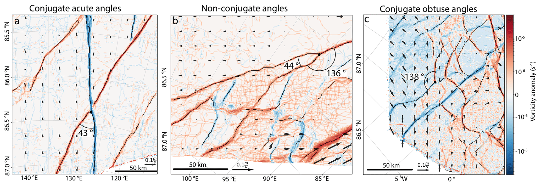
Figure 3 Examples of LKF intersections with the vorticity anomaly and sea-ice drift within the MOSAiC dataset. Panel (a) shows an intersection with an acute angle (1–2 January 2020), panel (b) shows an intersection with a non-conjugate angle (11–12 November 2019), and panel (c) shows an intersection with an obtuse angle (15–16 March 2020). The arrows indicate the velocity anomaly of the sea-ice drift calculated for the displayed data. Detected LKFs are plotted as thin black lines. The color bar of the vorticity anomaly is the same for all panels.

In the following, we focus on intersection angles between conjugate LKFs, which we can classify as acute or obtuse. We include only LKFs that formed during the same time step of observation.

3.2 Intersection angles

Figure 4 shows the probability density function (PDF) of the intersection angle of conjugate LKFs for the MOSAiC and RGPS datasets. The PDF of both datasets agrees remarkably well. Both IADs peak at acute angles, with a modal value in the range between 40 and 50^∘. Moreover, we find only a few large angles. For both datasets, around 80 % of the conjugate angles are acute, with around 25 % of them ranging between 30 and 60^∘.

To characterize the PDF, we fit both PDFs to an exponentially modified Gaussian (exGaussian) distribution with a maximum likelihood estimator (MLE). The parameters of the fit are given in the caption of Fig. 4. The formula of the exGaussian distribution is as follows:

$$\begin{array}{}\text{(1)}& f(x;\mathit{\mu },\mathit{\sigma },\mathit{\tau })={\displaystyle \frac{\mathrm{1}}{\mathrm{2}\mathit{\tau }}}{e}^{\frac{\mathrm{1}}{\mathrm{2}\mathit{\tau }}(\mathrm{2}\mathit{\mu }+\frac{{\mathit{\sigma }}^{\mathrm{2}}}{\mathit{\tau }}-\mathrm{2}x)}\mathrm{erfc}\left({\displaystyle \frac{\mathit{\mu }+\frac{{\mathit{\sigma }}^{\mathrm{2}}}{\mathit{\tau }}-x}{\sqrt{\mathrm{2}}\mathit{\sigma }}}\right),\end{array}$$

where

$$\begin{array}{}\text{(2)}& \mathrm{erfc}\left(x\right)={\displaystyle \frac{\mathrm{2}}{\sqrt{\mathit{\pi }}}}\underset{x}{\overset{\mathrm{\infty }}{\int }}{e}^{-t^{\mathrm{2}}}\mathrm{d}t.\end{array}$$

The goodness of the fit is tested with a Monte Carlo test with 10 000 different random subsamples, considering the discrete nature of intersection angles between LKFs that are defined on a regular grid (Hutter et al., 2019a), and using a Kolmogorov–Smirnov (KS) statistic (see details in Clauset et al., 2009; Hutter et al., 2019a). We also tested the logarithmic normal distribution and the skew normal distribution, but these fits failed the Monte Carlo test. The fitted exGaussian distributions show a modal peak at ${\mathrm{49}}^{\circ }\pm {\mathrm{1}}^{\circ }$ for the RGPS dataset and at ${\mathrm{42}}^{\circ }\pm {\mathrm{4}}^{\circ }$ for the MOSAiC dataset (Fig. 4). Considering the different spatial and temporal resolutions as well as the different ice regimes sampled, this agreement is remarkable and allows us to generalize conclusions on sea-ice properties.

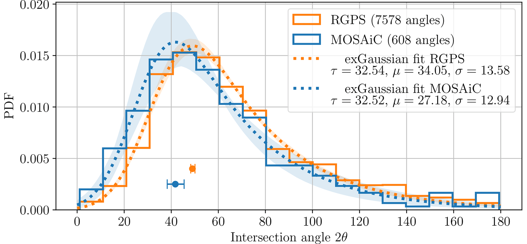
Figure 4 Probability density function of the conjugate intersection angles for the MOSAiC (blue) and RGPS (orange) datasets. The dashed lines show the MLE fit to an exponentially modified Gaussian (exGaussian) distribution (Eq. 1), and the fitted distribution parameters are shown in the legend. The shading shows the 1σ error of the distribution fits. We show the position of the distribution's peak with its 1σ error: ${\mathrm{49}}^{\circ }\pm {\mathrm{1}}^{\circ }$ for the RGPS dataset and ${\mathrm{42}}^{\circ }\pm {\mathrm{4}}^{\circ }$ for the MOSAiC dataset.

The PDF of the intersection angles does not vary seasonally for the RGPS dataset. For the MOSAiC dataset, there are too few intersection angles to study seasonal variations (not shown). Appendix A presents and discusses the PDF of non-conjugate intersection angles.

3.3 Divergence and convergence along leads

We extract the deformation rates from all pixels defined as part of an LKF to compare the characteristics of the deformation in the MOSAiC and RGPS datasets. As for the IAD, both the MOSAiC and RGPS datasets agree with respect to the shape of the distribution of the divergence, shear, and total deformation rates along LKFs (Fig. 5a, b, and c, respectively). As RGPS and MOSAiC differ with respect to their spatial resolution (by 1 order of magnitude) and deformation rates are known to be scale dependent, we normalize the divergence and shear to compare the relative frequencies. On average, we find more divergent ice motion along LKFs in the MOSAiC dataset compared with the RGPS dataset (Fig. 5a). We speculate that this reflects a generally more divergent regime in the Transpolar Drift compared with the Beaufort Gyre, which features more compressive settings. The RGPS dataset shows higher shear deformation that could potentially originate from the circular motion of the Beaufort Gyre. The higher shear rates also result in higher total deformation rates in the RGPS dataset.

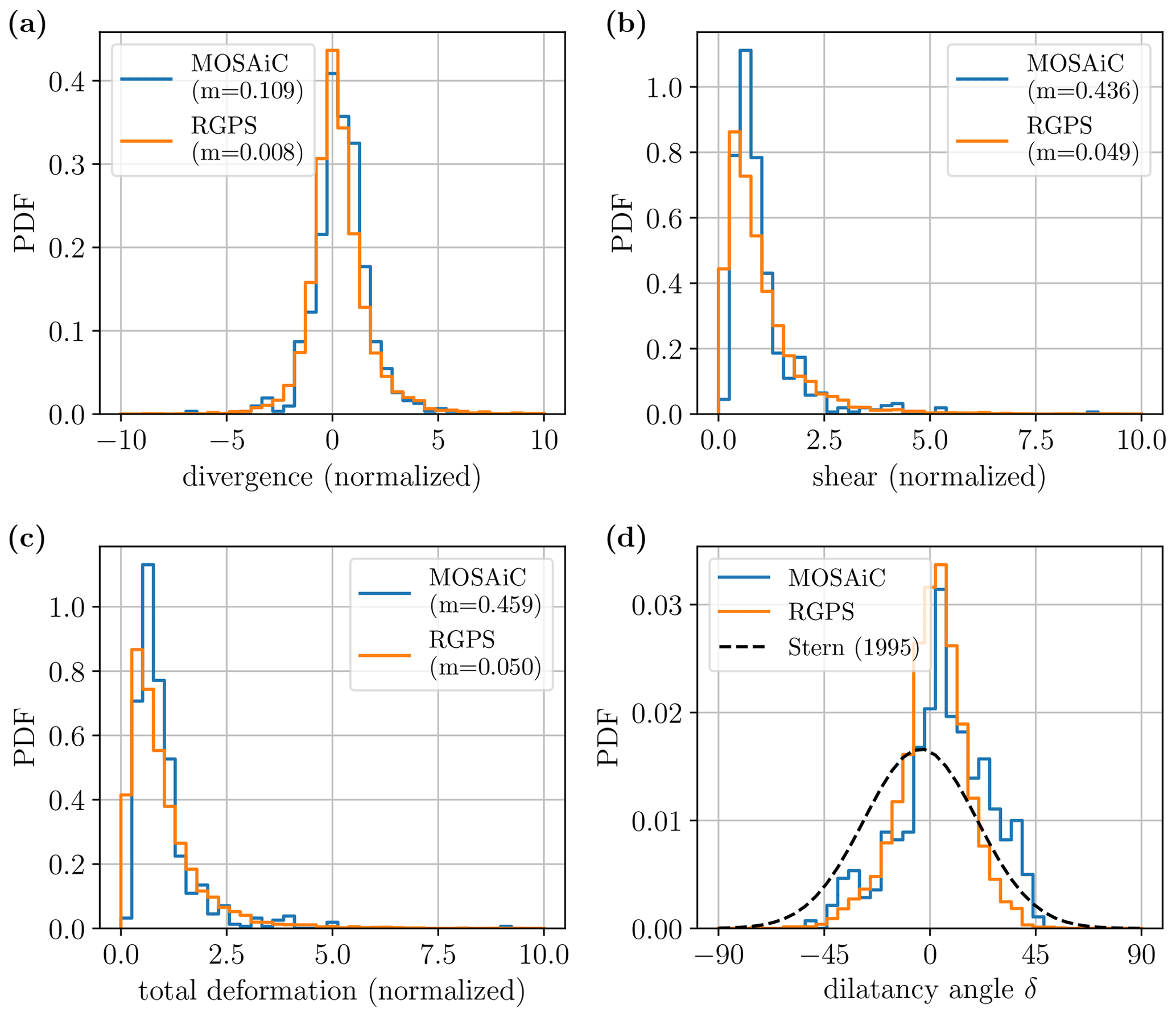
Figure 5 Probability distribution function of normalized convergence (a), normalized divergence (b), and normalized total deformation (c) along failure lines, as well as the dilatancy angle $\mathit{\delta }={\tan }^{-\mathrm{1}}\left(\frac{{\dot{\mathit{ϵ}}}_{\mathrm{div}}}{{\dot{\mathit{ϵ}}}_{\mathrm{shear}}}\right)$ (d). The means used for the normalization are given in parentheses in the legend. The black curve in panel (d) shows the Gaussian curve with the parameters presented in Stern et al. (1995, their Fig. 4) for comparison.

We can calculate the dilatancy angle along the LKF, δ, i.e., the angle of deformation defined by the ratio of shear and divergence $\tan \left(\mathit{\delta }\right)=\frac{{\dot{\mathit{ϵ}}}_{\mathrm{div}}}{{\dot{\mathit{ϵ}}}_{\mathrm{shear}}}$ (Tremblay and Mysak, 1997). Here, the divergence and shear are used before normalization. The presence of smaller dilatancy angles in the distribution (Fig. 5d) shows that divergence more frequently occurs in the MOSAiC dataset (Fig. 5d).

Further, we analyze the relationship between intersection angles and dilatancy angles (Fig. 6). We find a weak correlation between the intersection angle and the dilatancy angle, with a correlation coefficient of $\mathit{\rho }=-\mathrm{0.5}$ for MOSAiC and a very weak correlation of $\mathit{\rho }=-\mathrm{0.2}$ for RGPS. The theory of Roscoe angles θ_R (Roscoe, 1970) states that the dilatancy (i.e., the orientation of the flow rule) controls the orientation of the LKFs. In doing so, intersection angles 2θ can be described as a function of the dilatancy angle δ and vice versa by

$$\begin{array}{}\text{(3)}& \mathrm{2}\mathit{\theta }=\arccos \left(\tan \right(\mathit{\delta }\left)\right),\end{array}$$

shown as a red dashed line in Fig. 6. In contrast to theory, we find that both PDFs are not linked following this functional form (Fig. 6), showing only weak correlations (ρ_R=0.46 for MOSAiC and ρ_R=0.20 for RGPS) and even negative determination coefficients (R² values), meaning that a constant value would be a better fit than Eq. (3).

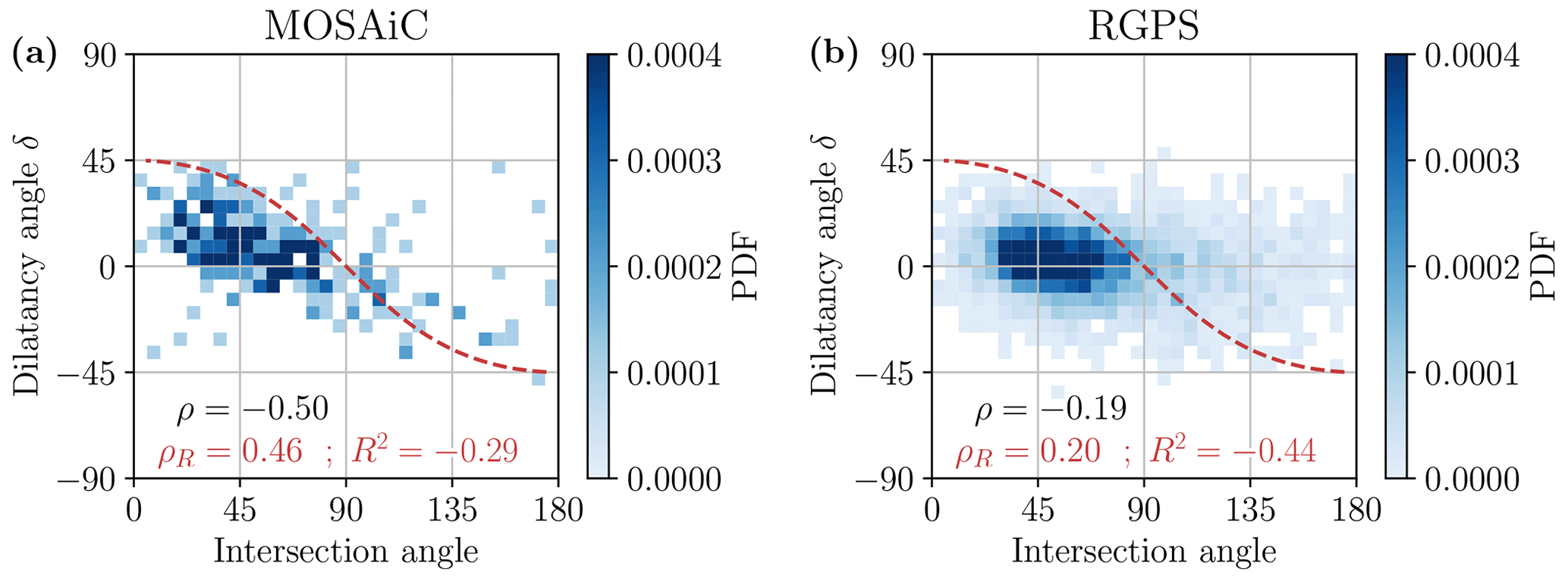
Figure 6 Scatterplot of the dilatancy angle δ versus the intersection angles between LKFs. The correlation between the intersection angle and the dilatancy angle is $\mathit{\rho }=-\mathrm{0.5}$ for MOSAiC and $\mathit{\rho }=-\mathrm{0.19}$ for RGPS. The dashed red line shows the relationship between dilatancy and angles expected following a normal flow rule or the Roscoe angle theory. The correlations between this prediction and the observed dilatancy angles are ρ_R=0.46 for MOSAiC and ρ_R=0.20 for RGPS. All correlations are significant.

These findings contradict the concept of the Roscoe angle θ_R and the idea of a normal flow rule, as we observe only weak correlations between intersection angles and dilatancy angles. However, we note that the MOSAiC dataset holds a higher correlation than the RGPS dataset. Thus, the non-correlations could arise from an observational bias due to the low temporal resolution. Therefore, increasing the temporal resolution might show a correlation, as it would resolve the deformation just after failure. Finally, we note that our observations confirm the theoretically expected range of the dilatancy angle: as expected from Roscoe's theory and the normal flow rule condition, dilatancy angles lower than 45^∘ and above 135^∘ are very rare in our observations (Figs. 5d and 6).

3.4 Mechanical properties of sea ice

3.4.1 Estimation of the internal angle of friction

The peak of the IAD shows a preferred angle of failure of sea ice that can be used to estimate the internal angle of friction of sea ice within the framework of the Mohr–Coulomb failure criterion (Coulomb, 1776). The internal angle of friction is the ratio of shear stress τ and normal stress σ at which the material yields.

The internal angle of friction is given by $\mathit{\varphi }=\frac{\mathit{\pi }}{\mathrm{2}}-\mathrm{2}\mathit{\theta }$, where 2θ is the peak of the IAD. Within the Coulombic framework, the internal angle of friction is linked to a Coulombic shear criterion, such as

$$\begin{array}{}\text{(4)}& \mathit{\tau }=\mathit{\mu }\mathit{\sigma }+{\mathit{\tau }}_{\mathrm{0}},\end{array}$$

where μ=tan (ϕ) and τ₀ is the cohesion, i.e., the shear strength. Similarly, the criterion can be translated in invariant stress space (σ_I,σ_II) for the construction of a yield curve (Ringeisen et al., 2019) and is given by

$$\begin{array}{}\text{(5)}& {\mathit{\sigma }}_{\mathrm{II}}={\mathit{\mu }}_{\mathrm{I}}{\mathit{\sigma }}_{\mathrm{I}}+c_{\mathrm{I}},\end{array}$$

where μ_I=sin (ϕ).

Using these formulas with the observed IAD from our study, we find the following:

• The peak intersection angle for the RGPS dataset of $\mathrm{2}\mathit{\theta }={\mathrm{49}}^{\circ }\pm {\mathrm{1}}^{\circ }$ implies an internal angle of friction of $\mathit{\varphi }={\mathrm{41}}^{\circ }\pm {\mathrm{1}}^{\circ }$, $\mathit{\mu }=\mathrm{0.87}\pm \mathrm{0.03}$, and ${\mathit{\mu }}_{\mathrm{I}}=\mathrm{0.66}\pm \mathrm{0.02}$.

• For the MOSAiC dataset, for the intersecting angle of $\mathrm{2}\mathit{\theta }={\mathrm{42}}^{\circ }\pm {\mathrm{4}}^{\circ }$, we get $\mathit{\varphi }={\mathrm{48}}^{\circ }\pm {\mathrm{4}}^{\circ }$, $\mathit{\mu }=\mathrm{1.12}\pm \mathrm{0.15}$, and ${\mathit{\mu }}_I=\mathrm{0.75}\pm \mathrm{0.05}$.

Note that we only take the peak of the IAD into account for this calculation, thereby neglecting the presence of other intersection angles in the PDF.

3.4.2 Estimation of the shape of a yield curve or a plastic potential

Instead of using only a single angle to derive the mechanical properties of sea ice, we can also use the complete PDF of the intersection angles (Fig. 4) to create an approximation of the shape of the yield curve or plastic potential within the VP framework. In the following, we consider that the curve that we derive can be a yield curve or a plastic potential, as there is still an open question regarding which of these mechanical properties sets the intersection angles of LKFs in sea-ice plastic models, although there are indications that the plastic potential could be responsible (Ringeisen et al., 2021). To reconstruct these curves from the IAD, we follow the results of Wang (2007), Ringeisen et al. (2019), or Ringeisen et al. (2021). The slope of different parts of the yield curve (Coulomb angle) or plastic potential (Roscoe angle) are linked to different intersection angles:

$$\begin{array}{}\text{(6)}& \mathrm{2}\mathit{\theta }=\arccos \left(-{\displaystyle \frac{\partial {\mathit{\sigma }}_{\mathrm{II}}}{\partial {\mathit{\sigma }}_{\mathrm{I}}}}\right),\end{array}$$

where the function σ_II(σ_I) defines the yield curve or the plastic potential in the invariant stress space (σ_I,σ_II). In the following, we hypothesize that the number of intersecting LKFs within a bin of angles is proportional to the length of the yield curve/plastic potential curve that creates this angle. Here, our underlying hypothesis is that all of the points on the yield curve/plastic potential are equally likely. An additional constraint is that the curve is required to be convex to agree with the convexity condition of Drucker's postulate of stability (Drucker, 1959).

For each bin of angles in the PDF of the intersection angles (Fig. 4), we compute a segment of the yield curve (or plastic potential) that has the length of the PDF value. Finally, we compute the slope given by the angle in the center of this bin θ_m by inverting Eq. (6):

$$\begin{array}{}\text{(7)}& {\displaystyle \frac{\partial {\mathit{\sigma }}_{\mathrm{II}}}{\partial {\mathit{\sigma }}_{\mathrm{I}}}}=-\cos \left(\mathrm{2}\mathit{\theta }\right).\end{array}$$

This process is illustrated in Fig. 7. We start the construction of the curve at the origin of the invariant stress (σ_I, ${\mathit{\sigma }}_{\mathrm{II}})=(\mathrm{0},\mathrm{0})$. We start from the smallest intersection angles of the distribution, as they are linked to the steepest curve slopes from Eq. (7), and iterate through the PDF, with the start point of each segment being the tip of the previous segment. Note that, as long as the intersection angles are either monotonically increasing or decreasing, our method necessarily leads to a convex yield curve. Finally, the curve values are normalized to have the tip at ${\mathit{\sigma }}_{\mathrm{I}}=-\mathrm{1}$. Figure 8 shows the resulting shape.

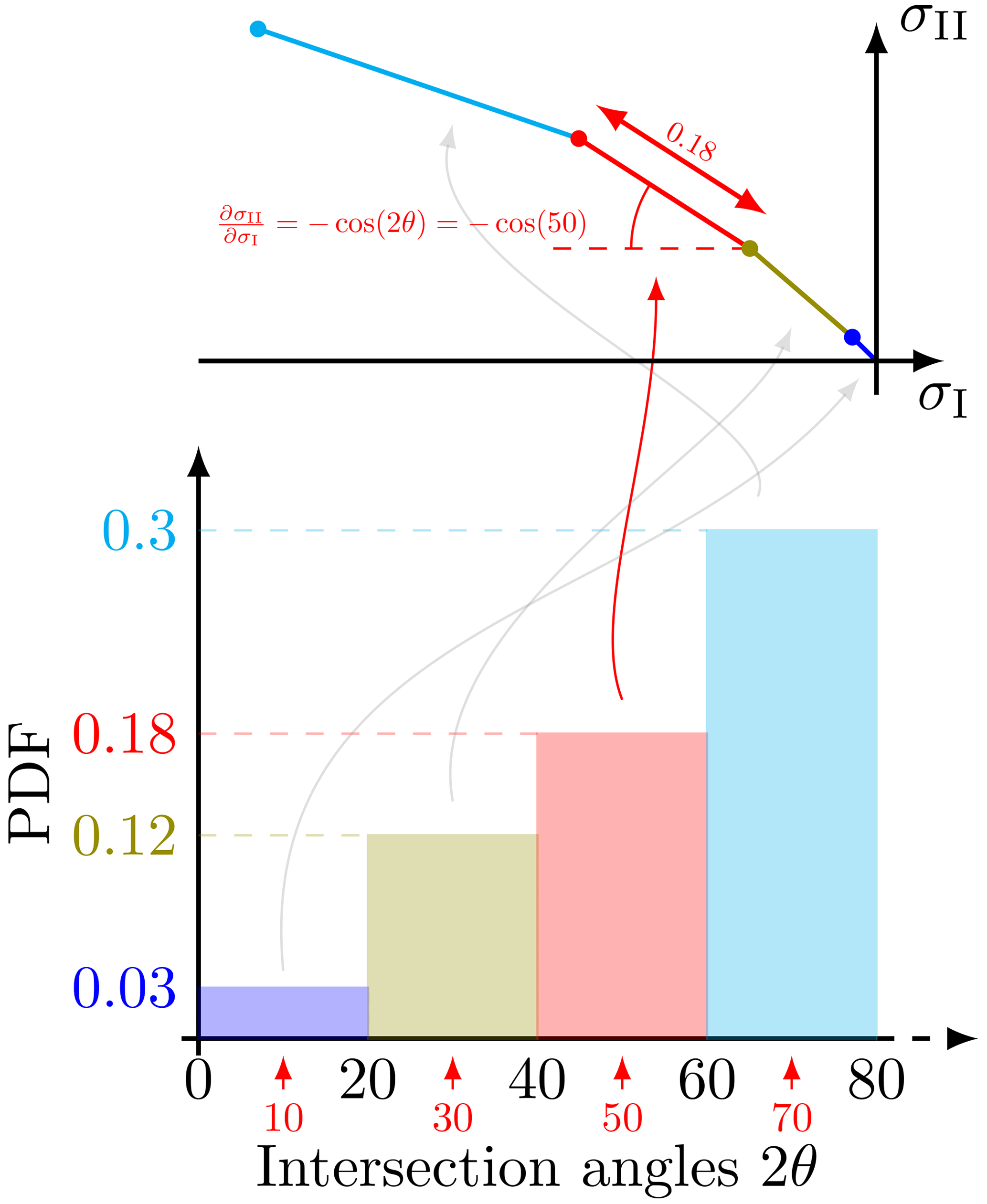
Figure 7 Example of the approximation method for the yield curve or plastic potential from the intersection angle distribution (IAD). Each bin of the distribution is used to create a segment of the curve with the length of the PDF value and the angle corresponding to the center of the bin, starting from the smaller bin.

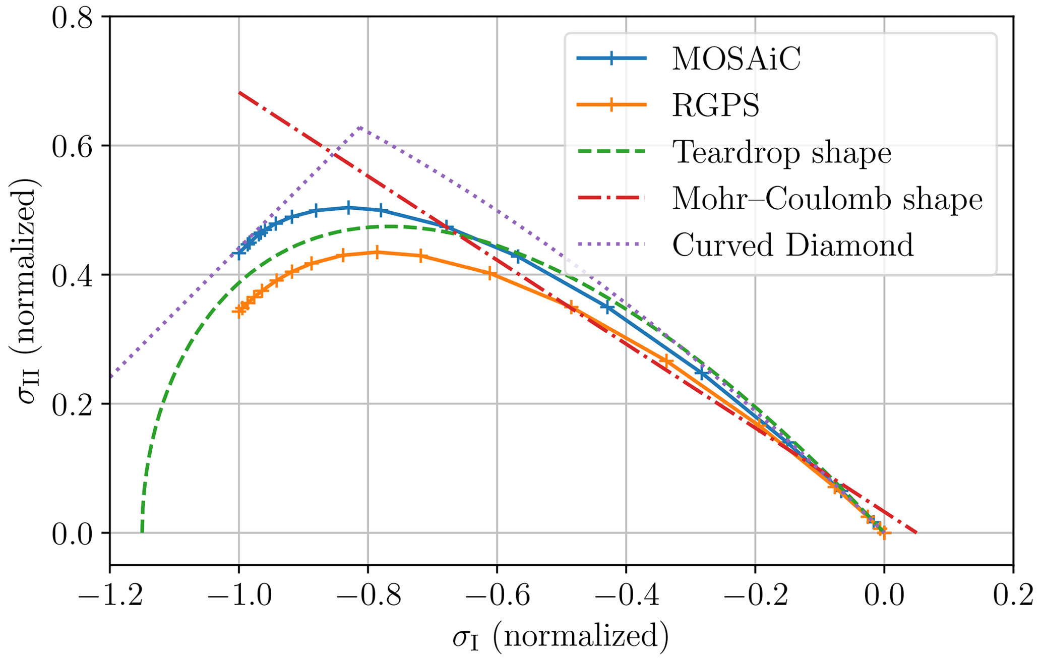
Figure 8 Yield curve or plastic potential constructed from the PDF of the intersection angles. The red dot-dash line, the green dashed line, and the violet dotted line show a Mohr–Coulomb yield curve (Tremblay and Mysak, 1997), a teardrop shape (Zhang and Rothrock, 2005; Ringeisen et al., 2022), and a curved diamond (Wang, 2007), respectively, for comparison. For the Mohr–Coulomb yield curve, the slope is μ=0.75, as derived in Sect. 3.4.1.

The estimations of the obtained curves for the RGPS and MOSAiC datasets resemble a teardrop yield curve (Zhang and Rothrock, 2005; Rothrock, 1975; Ringeisen et al., 2022), a Mohr–Coulomb yield curve (Ip et al., 1991), or (to a lesser extent) the curved diamond yield curve (Wang, 2007), but they clearly deviate from the elliptical yield curve (see Appendix B). For comparison, we added a teardrop, a Mohr–Coulomb, and a curved diamond yield curve in Fig. 8.

Note that the starting point of our curve is arbitrarily placed at the origin, as we did not consider tensile strength. However, adding tensile strength would not change the shape of the curve, which is central, but only the actual values of σ_I and σ_II. In other words, the shape of the curve is important, not its position in the (σ_I, σ_II) space.

In Appendix B, we present a proof of concept of this method. Using the IAD measured in three 2 km simulations with the Massachusetts Institute of Technology general circulation model (MITgcm; Hutter et al., 2022), we show that the yield curves reconstructed with the presented method agree well with the elliptical yield curves used in the simulations.

4 Discussion

We show the intersection angle distribution (IAD) of conjugate faults in Arctic sea ice during faulting events. The IAD shows the predominance of small intersection angles of 30 to 60^∘. The predominance of small angles agrees with the previous observations of intersection angles, which report angles between 28^∘ and 36^∘ (Erlingsson, 1988; Marko and Thomson, 1977; Walter and Overland, 1993; Cunningham et al., 1994). However, our observations show that wider angles, even obtuse angles, are also present in sea ice, although less frequently. The spread and shape of the IAD can be explained by the presence of heterogeneities in the ice (open or refrozen leads, ridges, and polynyas) that influence the orientation of LKFs (Wilchinsky and Feltham, 2011) or by variations in the internal confining pressure (Golding et al., 2010; Schulson et al., 2006). The heterogeneities serve as the preferred direction of ice failure and, therefore, can alter the intersection angle from the single angles of Mohr–Coulomb theory. We note that the IADs of the RGPS and MOSAiC datasets look very similar in shape. Given the different scales, times, and regions of the datasets, we conclude that the shape of the IAD seems to be a characteristic of sea ice. Future work should investigate how the shape of the IAD is linked to other typical characteristics of sea ice, like the shape of the floe size distribution (Rothrock and Thorndike, 1984; Stern et al., 2018) and the shape of the ice thickness distribution (von Albedyll et al., 2022; Thorndike et al., 1975).

Using the peak of the IAD, we made an estimation of the internal angle of friction from the Mohr–Coulomb framework. Our estimates of μ_I=0.66 and μ=0.75 agree well with previous estimates of the internal angle of friction $\mathit{\mu }\in [\mathrm{0.6},\mathrm{0.8}]$ by Schulson et al. (2006). In contrast, our estimates disagree with the findings of Erlingsson (1988, 1991). Applying a breaking index of i=2, defined by the Erlingsson (1988, 1991) methodological framework, the estimated internal angles of friction are $\mathit{\varphi }\simeq {\mathrm{25}}^{\circ }$ or μ≃0.13 and $\mathit{\varphi }\simeq {\mathrm{65}}^{\circ }$ or μ≃0.82. However, as we find that this framework does not agree with the creation of LKFs in sea-ice models, we rather focus on the Mohr–Coulomb framework. More importantly, we used the IAD to derive an approximation of a yield curve/plastic potential for sea-ice VP models. Wang (2007) used a similar method to create the curved diamond yield curve, although with fewer angle observations and a strong assumption about inferring the unknown stress direction from coastal geometry. Using the along-lead vorticity, we know the main stress direction and can do without such assumptions. The shape resulting from our analysis is similar to a teardrop shape (Rothrock, 1975; Zhang and Rothrock, 2005; Ringeisen et al., 2022), a Mohr–Coulomb shape (Ip et al., 1991), or (to a lesser extent) a curved diamond (Wang, 2007). In contrast, the shape that we obtain does not fit the elliptical shape (Hibler, 1979) or the parabolic lens shape (Zhang and Rothrock, 2005). These findings are of great relevance for designing new rheologies for sea-ice models. In this context, the observed IAD can be also used as a metric to assess models' capability to represent LKFs.

In VP models, the orientation of the LKFs is tightly linked to the flow rule, i.e., the dilatancy or post-failure deformation, at least for the elliptical yield curve and plastic potentials (Ringeisen et al., 2021). The observations presented here show no strong relationship between the observed dilatancy angle and the observed intersection angle nor between the dilatancy angles and the expected angles from Roscoe theory (Roscoe, 1970) or the normal flow rule. We consider insufficient observations or a general flaw in the VP rheological framework as potential reasons for this misfit between theory and observations. First, the temporal resolution of our observations might be insufficient to resolve double-sliding cycles with positive and negative dilatancy (Balendran and Nemat-Nasser, 1993). In that case, we would not see the immediate post-fracture deformation but rather the sliding of ice packs that alternate between dilatation and compression. This would lead to a random distribution of dilatancy angles and, thus, a decorrelation. We suggest further observational studies with a higher temporal resolution to confirm the decorrelation. Second, if confirmed by observations at higher temporal resolution, uncoupling between dilatancy and intersection angles would mean that the intersection angle is not influenced by the velocity characteristics of the medium. A confirmed uncoupling would question the capacity of the VP rheological framework to reproduce both the dilatancy and the LKF intersection angles simultaneously.

The presented results of the IAD are robust in scale, resolution, and geographic area. The RGPS dataset has low spatial and temporal resolution but a large spatial and time coverage, whereas the MOSAiC dataset has higher resolution but only covers the track of the MOSAiC drift experiment. The scale independence of the intersection angles agrees with the self-similarity and scaling properties of sea-ice deformation (Rampal et al., 2008; Weiss, 2013; Marsan et al., 2004; Bouchat and Tremblay, 2020; Hutchings et al., 2011). While the LKFs at the kilometer-scale resolution that we analyzed in this study are mostly systems of smaller-scale leads, a question remains regarding whether the observed deformation characteristics and IADs are still present at the floe scale (<100 m). Observational scaling studies analyzing sea-ice deformation derived from ship radar have shown that sea-ice deformation follows the same scaling behavior down to scales of 50 m (Oikkonen et al., 2017). This and laboratory experiments at a sub-meter scale (Schulson et al., 2006; Weiss and Dansereau, 2017) indicate similar failure behavior across scales and, therefore, no scale break. However, scaling characteristics are known to be only weakly linked to the representation of LKF intersection angles (Hutter et al., 2022) and, therefore, are potentially a poor proxy for the floe-scale IAD. Deformation derived from the shipborne ice radar from the MOSAiC drift experiment could bridge the gap in the scale analysis of the LKF intersection angle and give insight into the small-scale processes involved (rotation and reopening of leads), owing to its high temporal (2 s–10 min) and spatial (10 m) resolution in the proximity (approx. 9 km) of the ship (Krumpen et al., 2021a).

5 Conclusions

Using the vorticity in sea-ice deformation, we show that we can separate obtuse and acute intersection angles between sea-ice linear kinematic features (LKFs). Using this technique, we can now extract the probability density function (PDF) of the intersection angles between 0 and 180^∘, instead of being limited to the range between 0 and 90^∘. We investigate intersection angles within two different deformation datasets: the RADARSAT RGPS product (Hutter et al., 2019b) and the MOSAiC dataset from Sentinel-1A and -1B (von Albedyll and Hutter, 2023).

The PDFs of intersection angles show that acute angles dominate in both datasets, with PDFs peaking at 48^∘ (RGPS) and 45^∘ (MOSAiC). Both PDFs are described by an exponentially modified Gaussian distribution that agrees remarkably with respect to shape. Therefore, we conclude that the intersection angle distribution (IAD) is scale invariant. The distributions of divergence and shear rates along the LKFs also agree when taking the scaling of deformation rates into account. Both indicate scale-invariant behavior of fracture mechanics and intersection angles that remain to be tested at the floe scale. We do not find a relationship between the dilatancy angles along the leads and their corresponding intersection angles, which could be an artifact of the temporal resolution of a minimum of 1 d that might “smear” the deformation during instantaneous failure with post-fracture sliding. If not falsified with deformation data at very high temporal resolution, e.g., ship radar, the decorrelation of dilatancy and intersection angles contradicts the normal flow rule assumption used within the VP framework.

We infer the mechanical properties of sea ice from the observed IAD. Following methods from previous papers, we estimate the internal angle of friction to be ${\mathit{\mu }}_{\mathrm{I}}=\mathrm{0.66}\pm \mathrm{0.02}$ and ${\mathit{\mu }}_{\mathrm{I}}=\mathrm{0.75}\pm \mathrm{0.05}$ from the PDF peak for the MOSAiC and RGPS datasets, respectively. We outline a new method to derive the shape of the yield curve/plastic potential from the shape of the intersection angle PDF. The resulting shape agrees well with the shape of the teardrop yield curve (Zhang and Rothrock, 2005; Ringeisen et al., 2022), the Mohr–Coulomb curve (Ip et al., 1991), and (to a lesser extent) the curved diamond (Wang, 2007). We conclude that the popularly used elliptical yield (Hibler, 1979) is not backed by our observations.

Reproducing the observed patterns of LKFs in Arctic sea ice is one of the remaining challenges of the sea-ice modeling community (Hutter et al., 2022). Here, we provide an observed IAD that can be used as a metric for the evaluation of models, and we suggest replacing the elliptical yield curve in VP models with a teardrop yield curve for a better representation of simulated LKFs. Such a new setup will need to be tested in high-resolution Arctic simulations to determine if it represents the IAD observed in this study accurately.

Appendix A: Non-conjugate angles

In Sect. 3.4.1, we show that it is possible to separate the acute and the obtuse angles for 37 % of the intersection angles (28 % for MOSAiC and 38 % for RGPS). However, for many intersecting LKFs, the LKF vorticities are the same and it is not possible to separate between obtuse and acute angles (see Fig. 2b). Figure A1 shows the IAD for all angles, conjugate angles, and non-conjugate angles. Note that these PDFs are mirrored relative to 90^∘, as we cannot differentiate between obtuse and acute angles. For the RGPS dataset, extracting the non-conjugate angles leads to a very uniform IAD: there is still a peak in the IAD, but it is much less dominant. For the MOSAiC dataset, the non-conjugate angles feature many small angles, with peaks around 0 and 180^∘.

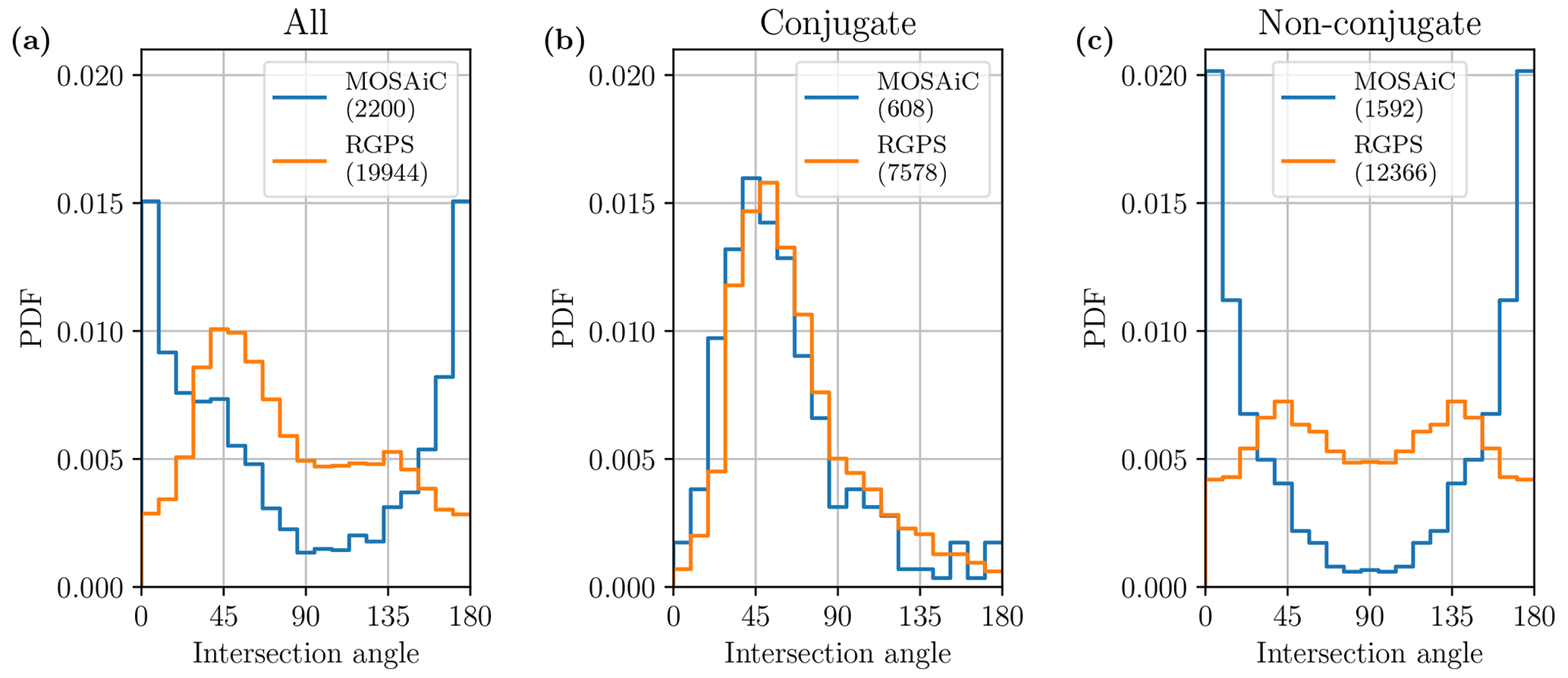
Figure A1 Probability density function (PDF) of the intersection angles in Arctic sea ice. The panels show the conjugate and non-conjugate angles for all (a), conjugate (b), and non-conjugate (c) angles, as defined in Fig. 2. The numbers in parenthesis show the numbers of intersection angles shown in the PDF.

The intersecting LKFs with the same vorticity can have several origins:

1. The time step of the observations is too large to resolve the actual vorticity during the deformation. The vorticity recorded over a (multi-)day-long period is not necessarily representative of the deformation rates during the formation. Even if two intersection LKFs are formed under compressive forcing, rapidly changing winds can induce a different ice motion. In this case, the initial failure allows the more mobile ice to deform in shear motion, which leads to the same vorticity sign. This behavior may be especially present for deformation data with a low temporal resolution, e.g., the RGPS dataset.

2. The presence of the same vorticity sign on both intersecting LKFs could emerge from rotation. LKF dynamics can involve rotation under shear (Wilchinsky and Feltham, 2004), which is a process also observed in granular materials (e.g., Oda and Kazama, 1998). This process seems more likely for small-scale observations, e.g., from the MOSAiC dataset with a spatial resolution of 1.4 km.

3. If an LKF is not detected properly and is cut into two parts, both parts will have the same sign vorticity and (due to their proximity) will be identified as intersecting LKFs in our analysis. We tuned the parameters of the detection algorithms to minimize this effect; however, especially for the MOSAiC data, we find instances of this effect.

Appendix B: Fracture angles from the elliptical yield curve

In the following, we show, as a proof of concept, that the method used in Sect. 3.4.2 allows for the reconstruction of the shape of the elliptical yield curve from the model deformation output. First, we compute the theoretical intersection angles' distribution from the yield curve shape. Then, we extract the intersection angles' distribution from 2 km resolution pan-Arctic simulations. Finally, we reconstruct the yield curve shape from the modeled intersection angles' distribution and show that it gives a shape very similar to the yield curve of the first step.

First, we compute the expected PDF of the intersection angles in a high-resolution sea-ice viscous–plastic model that uses an elliptical yield curve (Fig. B1a). For thousands of points on the yield curve, we compute the theoretical fracture angles, and we then use these points to create a theoretical intersection angle distribution. Figure B1c shows the results of this process for three different aspect ratios (e). The PDF of the intersection angles for e=2 peaks strongly at 90^∘. Using a smaller aspect ratio, such as e=0.7 (Bouchat and Tremblay, 2017) flattens the PDF. These PDFs are symmetrical relative to 90^∘, whereas the observations presented in this paper (Fig. 4) are strongly skewed towards small angles. Note that this process to estimate the IAD still uses the assumption that all parts of the yield curve are equally probable to be the subject of plastic deformation. An analysis of high-resolution sea-ice models would be necessary to see if this hypothesis is valid.

The histogram lines in Fig. B1c show the PDF of conjugate intersecting angles in a 2 km MITgcm simulation (Hutter et al., 2022) using the same method as described in Sect. 2.2. The histograms of simulated intersection angles show the same evolution of the PDF as expected from theory: a higher peak around 90^∘ for e=2 and a flatter PDF for e=1.0 and e=0.7. Furthermore, the PDFs of the models are close to being symmetrical with respect to 90^∘, despite using the algorithm to separate obtuse and acute angles.

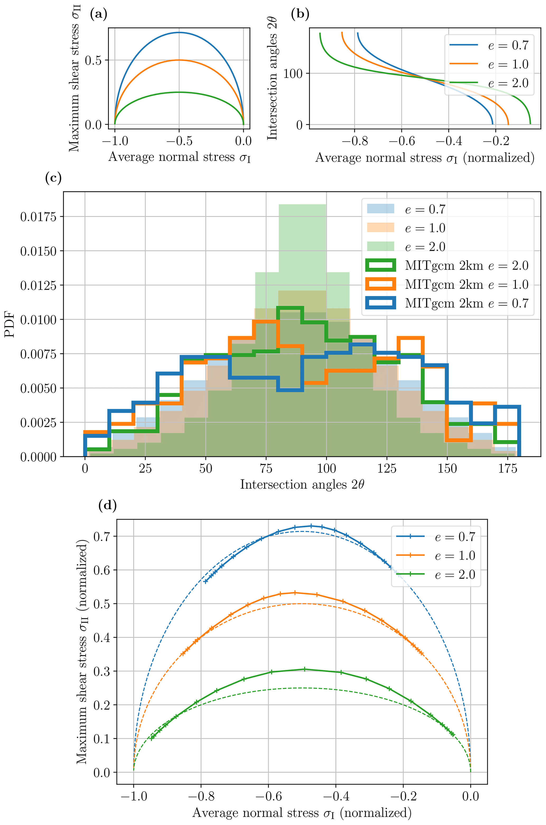
Figure B1 Elliptic yield curves in invariant space (a) and their theoretical fracture angle as a function of the first invariant σ_I (b); the PDF of the theoretical fracture angles, with the PDF of conjugate intersection angles from MITgcm 2 km resolution runs for the same ellipse ratios (c); and the reconstructed yield curve from the modeled IAD (d).

In Fig. B1d, we use the IAD from the simulations (Fig. B1c) to reconstruct the yield curve for all three values of e, as done in Sect. 3.4.2. The resulting yield curve fits well with the elliptical yield curve prescribed in the associated simulations. There is a larger difference for the e=2 case, and intersection angles around 90^∘ are less present than we would expect from the model. Globally, we see that all three PDFs of the modeled intersection angles are missing angles around 90^∘. This could be the results of a small departure from the hypothesis that all parts of the yield curve are equally probable. Note that LKF intersection angles can only be created when the slope of the yield curve is within the range $[-\mathrm{1},\mathrm{1}]$. A slope of −1 corresponds to an intersection angle of 0^∘, and a slope of +1 corresponds to an intersection angle of 180^∘. To take this into account, we start reconstructing the yield curve at the point [σ_I,σ_II], where $\frac{\partial {\mathit{\sigma }}_{\mathrm{II}}}{\partial {\mathit{\sigma }}_{\mathrm{I}}}=-\mathrm{1}$, and scale the rest of the yield curve to have the endpoint at σ_I, where the slope is $\frac{\partial {\mathit{\sigma }}_{\mathrm{II}}}{\partial {\mathit{\sigma }}_{\mathrm{I}}}=\mathrm{1}$.