the Creative Commons Attribution 4.0 License.
the Creative Commons Attribution 4.0 License.
 | 08 Sep 2023
Greenland and Canadian Arctic ice temperature profiles database
Kenneth D. Mankoff
Christian Zdanowicz
Gary D. Clow
Martin P. Lüthi
Samuel H. Doyle
Henrik H. Thomsen
David Fisher
Joel Harper
Andy Aschwanden
Bo M. Vinther
Dorthe Dahl-Jensen
Harry Zekollari
Toby Meierbachtol
Ian McDowell
Neil Humphrey
Anne Solgaard
Nanna B. Karlsson
Shfaqat A. Khan
Benjamin Hills
Robert Law
Bryn Hubbard
Poul Christoffersen
Mylène Jacquemart
Julien Seguinot
Robert S. Fausto
William T. Colgan
Here, we present a compilation of 95 ice temperature profiles from 85 boreholes from the Greenland ice sheet and peripheral ice caps, as well as local ice caps in the Canadian Arctic. Profiles from only 31 boreholes (36 %) were previously available in open-access data repositories. The remaining 54 borehole profiles (64 %) are being made digitally available here for the first time. These newly available profiles, which are associated with pre-2010 boreholes, have been submitted by community members or digitized from published graphics and/or data tables. All 95 profiles are now made available in both absolute (meters) and normalized (0 to 1 ice thickness) depth scales and are accompanied by extensive metadata. These metadata include a transparent description of data provenance. The ice temperature profiles span 70 years, with the earliest profile being from 1950 at Camp VI, West Greenland. To highlight the value of this database in evaluating ice flow simulations, we compare the ice temperature profiles from the Greenland ice sheet with an ice flow simulation by the Parallel Ice Sheet Model (PISM). We find a cold bias in modeled near-surface ice temperatures within the ablation area, a warm bias in modeled basal ice temperatures at inland cold-bedded sites, and an apparent underestimation of deformational heating in high-strain settings. These biases provide process level insight on simulated ice temperatures.
- Article
(7424 KB) - Full-text XML
-
Supplement
(280 KB) - BibTeX
- EndNote


With the tremendous social implications of sea level change, the past decade has seen a proliferation of simulations of the current and future geometry and dynamics of the Greenland ice sheet (Bindschadler et al., 2013; Goelzer et al., 2020; Aschwanden et al., 2021). These present-day complex ice flow models build upon the legacy of simpler past thermomechanical models (Letréguilly et al., 1991; Huybrechts et al., 1991; Funk et al., 1994; Calov and Hutter, 1996). Due to the high sensitivity of ice viscosity to ice temperature, the thermal state of the ice sheet is a critical element of these simulations (Colgan et al., 2015). At present, however, the englacial temperature fields of even cutting-edge ice sheet simulations remain largely unevaluated against observed temperatures (Aschwanden et al., 2019). While recent studies show potential for deriving internal ice temperatures from satellite or airborne data (Macelloni et al., 2019; Jezek et al., 2022), these techniques are not yet widely employed. There are consequently diverse opinions on Greenland's basal thermal state across the current generation of thermomechanical ice flow models (MacGregor et al., 2016, 2022).
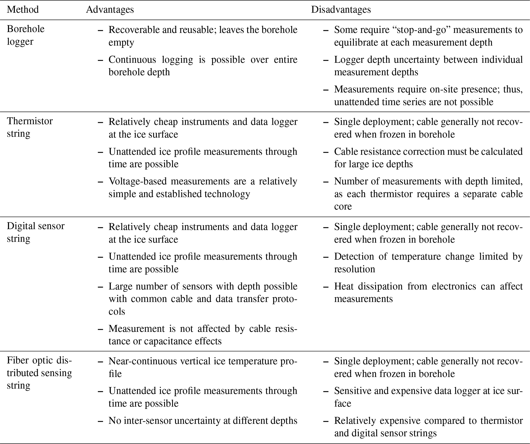
Several different methods for measuring ice temperatures have been used on the Greenland ice sheet and in the Canadian Arctic. The methods include the following: borehole logging, where a temperature sensor is moved up or down the borehole, measuring either “continuously” as the probe moves or stopping to measure at every depth (known as “stop-and-go”; Johnsen et al., 1995; Clow, 2008); sensor strings (this term includes both digital and analog), where thermistors are frozen into the ice, and ice temperatures are recorded at various depths at the same time (Iken et al., 1993; Ryser et al., 2014); and fiber optic distributed temperature sensing (DTS), where the ice temperature is measured near-continuously along the full cable length (Law et al., 2021). We summarize the methods and their advantages and disadvantages in Table 1.
Ice temperature profiles collected in Greenland and the Canadian Arctic have not been systematically compiled into a coherent database. In particular, many pre-1990 ice temperature profiles languished in non-digitized reports or gray literature. This presented a clear motivation to assemble ice temperature measurements into a consistent and comprehensive community resource. Here, we describe our compilation of ice temperature profiles from Greenland and the Canadian Arctic into an open-access database, with well-documented and uniform metadata for each entry. We include Canadian Arctic ice caps in our predominantly Greenland database, as these regions reside within the domain of some Greenland ice flow models (e.g., Tarasov and Peltier, 2004; Gowan et al., 2021).
The earliest temperature profile in our database is from 1950, when a 125 m profile was measured at Camp VI in West Greenland (Heuberger, 1954). Earlier temperature profiles may exist, and incorporating these profiles into the database is an ongoing process. We restrict our database to ice temperature profiles extending well below the depth of the seasonal temperature cycle. At cold, dry sites, this is often approximated to be 10 to 15 m below the surface (Cuffey and Paterson, 2010). Similar to a recent effort to compile surface mass balance observations into a readily accessible common framework (Machguth et al., 2016), we aim to create a community resource that facilitates comparisons between simulated and observed ice temperatures. Here, we describe the format of the database and the sources of our ice temperature data and metadata. We also discuss best practices for comparing observed ice temperatures with simulated ice temperatures from a 3-D thermomechanical model. Finally, we make an appeal to community colleagues to continually update this dataset and provide instructions for them to do so.
Table 1Advantages and disadvantages of the main methods for measuring deep-ice temperatures. This compilation ignores the absolute accuracy of the ice temperature sensor, which can vary greatly within any one method type.
The temperature database currently comprises a total of 95 temperature profiles. In two instances, the same borehole was logged twice at different times (Thomsen et al., 1991). Other boreholes which have been logged more than once also include GISP2-D, GISP2-G, NGRIP-2, NGRIP-S2, and NEEM-D; however, these are currently not included in the database. The database also contains partial temperature profiles, which are considered to make up one profile. This is the case for the two sites of FOXX6 and GULL1 (Ryser et al., 2014). Furthermore, five partial profiles at one site (Lüthi et al., 2002), all situated less than 25 m from one another, were also regarded as one borehole. This means that the 95 temperature profiles in the database are considered to originate from 85 unique boreholes.
See Fig. 1 for an overview of the drill site locations and the database for the complete list of borehole IDs. Borehole IDs denote the general location of the borehole, project-specific borehole IDs if multiple boreholes exist at that location, and the year of the measurement. Borehole temperature records were entered into the database in two different formats, namely (a) tabulated original measurements, provided either by community members or obtained from historical reports, or (b) published graphics of measured temperature profiles digitized using the publicly available digitization tool WebPlotDigitizer (https://automeris.io/WebPlotDigitizer, last access: 3 March 2022; Rohatgi, 2021).
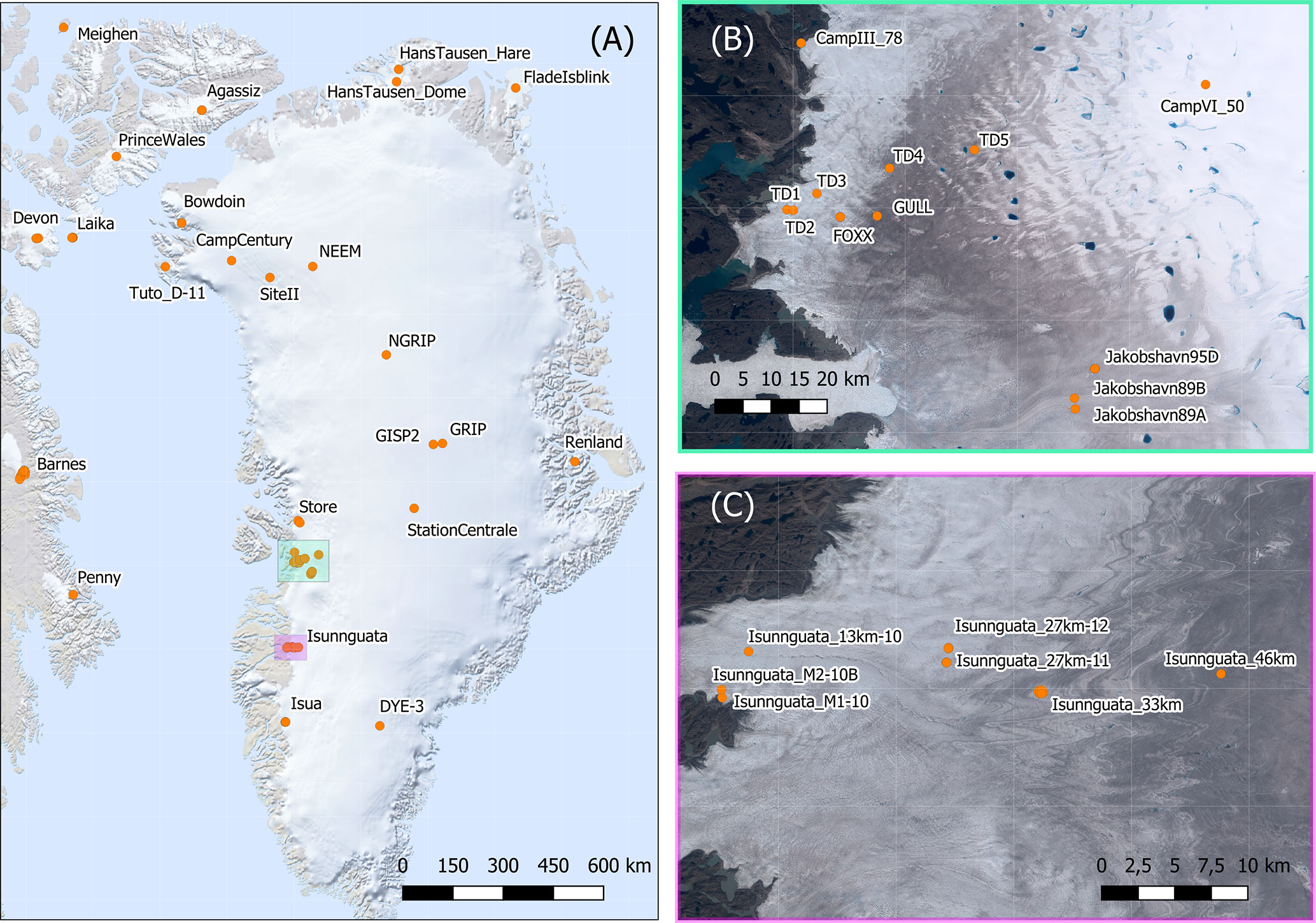
Figure 1(a) Overview of the drill site locations of temperature profiles contained in the database (plot created using QGreenland software; Moon et al., 2021). Note that for locations where several drill sites exist close to each other, only the common name is shown, e.g., Agassiz. The green and purple boxes indicate regions where numerous profiles have been drilled. (b) Enlarged view of the region near Jakobshavn Glacier. (c) Enlarged view of the region near Isunnguata Sermia glacier. Panels (b) and (c) show positions plotted on top of Sentinel-2 multispectral satellite imagery, with 10 m resolution, from 2019 (MacGregor et al., 2020). All maps are displayed in EPSG:3413 polar stereographic projection, with the easting and northing coordinates given in meters.
Overall, 71 of the 95 profiles were available as tabulated temperature measurements (Heuberger, 1954; Classen, 1977; Stauffer and Oeschger, 1979; Clarke et al., 1987; Thomsen et al., 1991; Iken et al., 1993; Hansson, 1994; Cuffey et al., 1995; Thomsen et al., 1996; Cuffey and Clow, 1997; Dahl-Jensen et al., 1998; Fischer et al., 1998; Lüthi et al., 2002; Kinnard et al., 2006; Buchardt and Dahl-Jensen, 2007; Kinnard et al., 2008; Lemark and Dahl-Jensen, 2010; Rasmussen et al., 2013; Ryser et al., 2014; Harrington et al., 2015; Hills et al., 2017; Zekollari et al., 2017; Doyle et al., 2018b; Seguinot et al., 2020; Hubbard et al., 2021a; Harper and Meierbachtol, 2021; Law et al., 2021). The remaining 24 profiles were digitized from figures (Hansen and Landauer, 1958; Davis, 1967; Paterson, 1968; Classen, 1977; Paterson et al., 1977; Colbeck and Gow, 1979; Gundestrup and Hansen, 1984; Blatter and Kappenberger, 1988; Gundestrup et al., 1993).
Here, we describe both the initial Dataverse database release (Mankoff et al., 2022) and the GitHub living repository (Mankoff, 2022). The Dataverse database (Mankoff et al., 2022) contains four curated files, namely two comma-separated value (CSV) files with temperature and depth-normalized temperature at each site, a Keyhole Markup Language (KML) file of borehole locations, and a metadata file. The GitHub living repository (Mankoff, 2022) is where raw data are collected, curated, and documented in order to create the final data. The repository is termed “living” because it is also the entry point for new data in future database versions.
The GitHub living repository (Mankoff, 2022) consists of high-level, post-processed CSV files ready for use and low-level folders with original sources and notes for each temperature profile. The CSV files include two data files combining all profiles, where one file has depth in units of meters with a step size of 1 m, and another file has normalized depth as 0–1 with a step size of 0.01. This standardization of the profiles from coarse discrete measurements to uniformly finely spaced values was done by interpolating between points, using cubic spline interpolation with no overshoot. A third CSV file combines all metadata for each profile, and finally, a geographic information system (GIS) file (format KML) provides borehole locations. Folders also contain a file named “data.csv” with the original data at the original depth resolution, a README.org file with any relevant notes, including “cleaned” email correspondence when personal communications were involved in recovering the data, or other files detailing the data acquisition.
Where ice temperature profiles are derived from a graphic (Barnes_(B4,D4)_1974, Barnes_T0(975_1976, 91_1977, 81_1978, 61_1977, and 20_1979), Camp Century, Devon72, Devon73, DYE-3, Isua_10-14, Laika_75a-75e, Meighen67, SiteII, and Tuto_D-11), the graphic is included in the folder. These folders also include a *.tar or *.JSON file which can be opened in WebPlotDigitizer; the file contains the digitized profile and shows the digitization method. Graphical temperature data were digitized in the following way: the figure was loaded into WebPlotDigitizer as an xy plot. The axis of the figure was then calibrated by defining two points on each axis, with these definition points preferably being as far away from each other as possible. The program has two options for digitizing, namely “manual” or “automatic” extraction, and typically a combination of both methods was used. Using the automatic mode, profiles were defined by creating a mask, and an automatic extraction was used to produce an initial set of points. The manual mode was then used to adjust these points where necessary to fine-tune a visual match to the graphic. For figures that contained both in situ temperature points and a fitted temperature line, only the points were detected using WebPlotDigitizer's “blob detector” automatic algorithm.
Digitizing data from graphics can introduce non-trivial digitization uncertainty associated with the potentially improper alignment of the defining axes (systematic uncertainty) and/or the improper alignment of the data points (random uncertainty). The magnitude of this digitization uncertainty is proportional to the sizes of the graphic and data range, which vary from profile to profile. To highlight the potential importance of the digitization uncertainty, we propagate the uncertainty associated with a ±2 pixel error in each of the axes, thus defining points for both temperature and depth in the digitized profiles with the thinnest ice (Tuto_D-11; 48 m) and the thickest ice (DYE-3; 2038 m). The Tuto_D-11 graphic (Davis, 1967; Fig. 2a) is ∼1000 pixels tall and spans 47.5 m, which yields a ±2 pixel depth uncertainty of ±0.15 m. The Tuto_D-11 graphic is ∼600 pixels wide and spans 32 ∘C, which yields a ±2 pixel temperature uncertainty of ±0.1 ∘C. In comparison, the DYE-3 graphic (Gundestrup and Hansen, 1984; Fig. 2b) is ∼1200 pixels tall, spans 2200 m and yields a ±2 pixel depth uncertainty of ±3.6 m. The DYE-3 graphic, ∼900 pixels wide, spans 8 ∘C and yields a ±2 pixel temperature uncertainty of ±0.02 ∘C. These end-member scenarios highlight how digitization uncertainty varies from graphic to graphic.
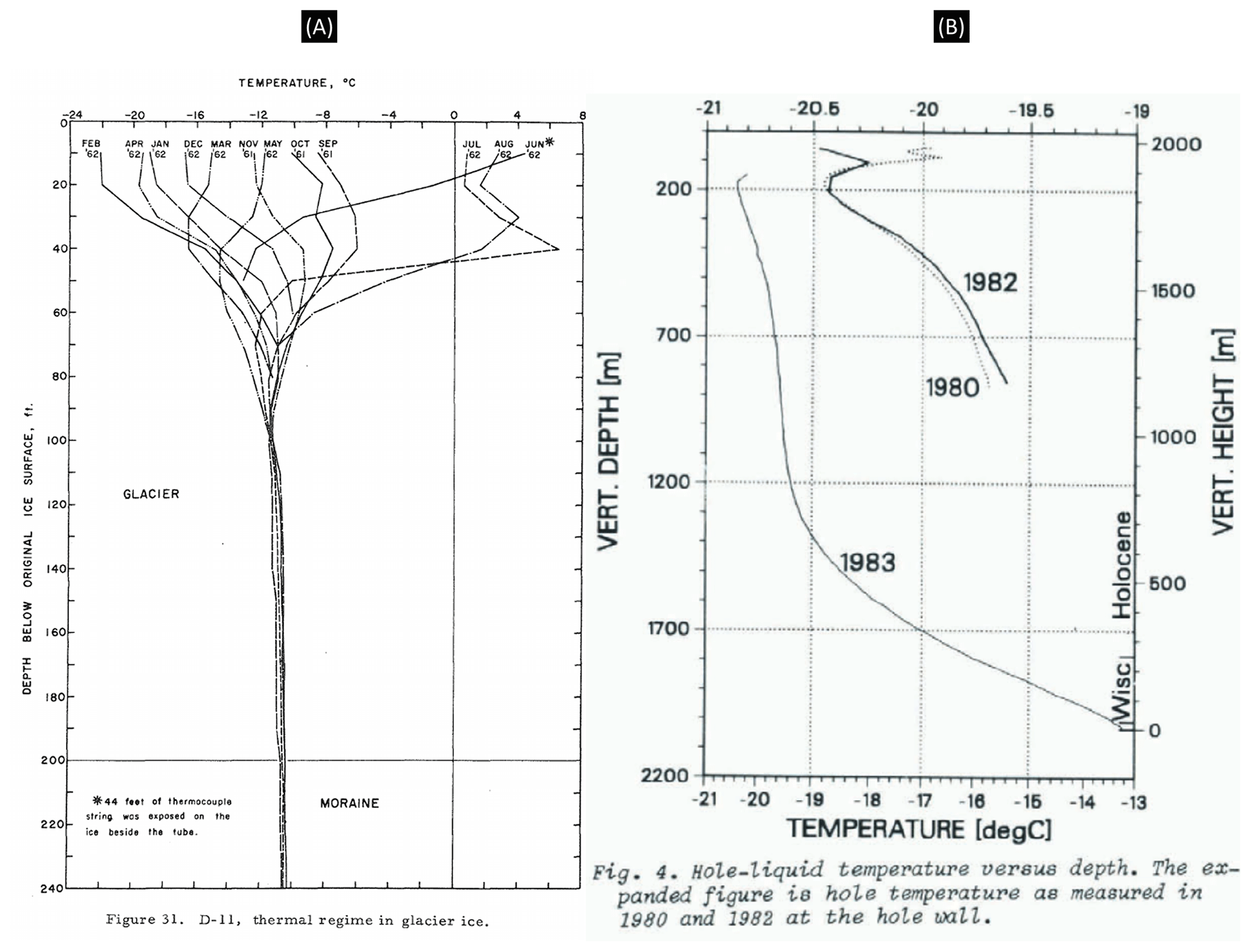
Figure 2(a) Graphic from which the Tuto_D-11 profile is digitized (Davis, 1967). This figure is reproduced from a U.S. government publication. (b) Graphic from which the DYE-3 profile is digitized (Gundestrup and Hansen, 1984). This figure is reproduced with permission from the International Glaciology Society.
All ice temperature profiles – from both digitized and tabulated sources – were standardized by interpolating between points, using cubic spline interpolation with no overshoot, in order to resolve the two common depth scales, namely the absolute depth scale at 1 m vertical resolution (Fig. 3a, c, e) and the normalized depth scale at non-dimensional 0.01 vertical resolution (Fig. 3b, d, f). The latter allows easy comparison between sites of different ice thicknesses and is useful for overcoming slight differences in ice thickness when comparing observed and modeled temperature profiles. The normalized depth-scale temperature file is named “temperature_dnorm.csv”. The absolute depth-scale temperature file, which is expressed as temperature with depth from the surface, is named “temperature.csv”. In each file, “NaN” means that no temperature data are available at the given depth, and in the absolute depth file, “−999” refers to an elevation below bedrock. Ice thicknesses vary significantly across the database profiles, from 3085 m at NGRIP to 48 m at Tuto_D-11, so the number of −999 below-bed null values varies between sites. This is because the temperature vector length is constant across the database entries, but the ice thickness varies across database entries.
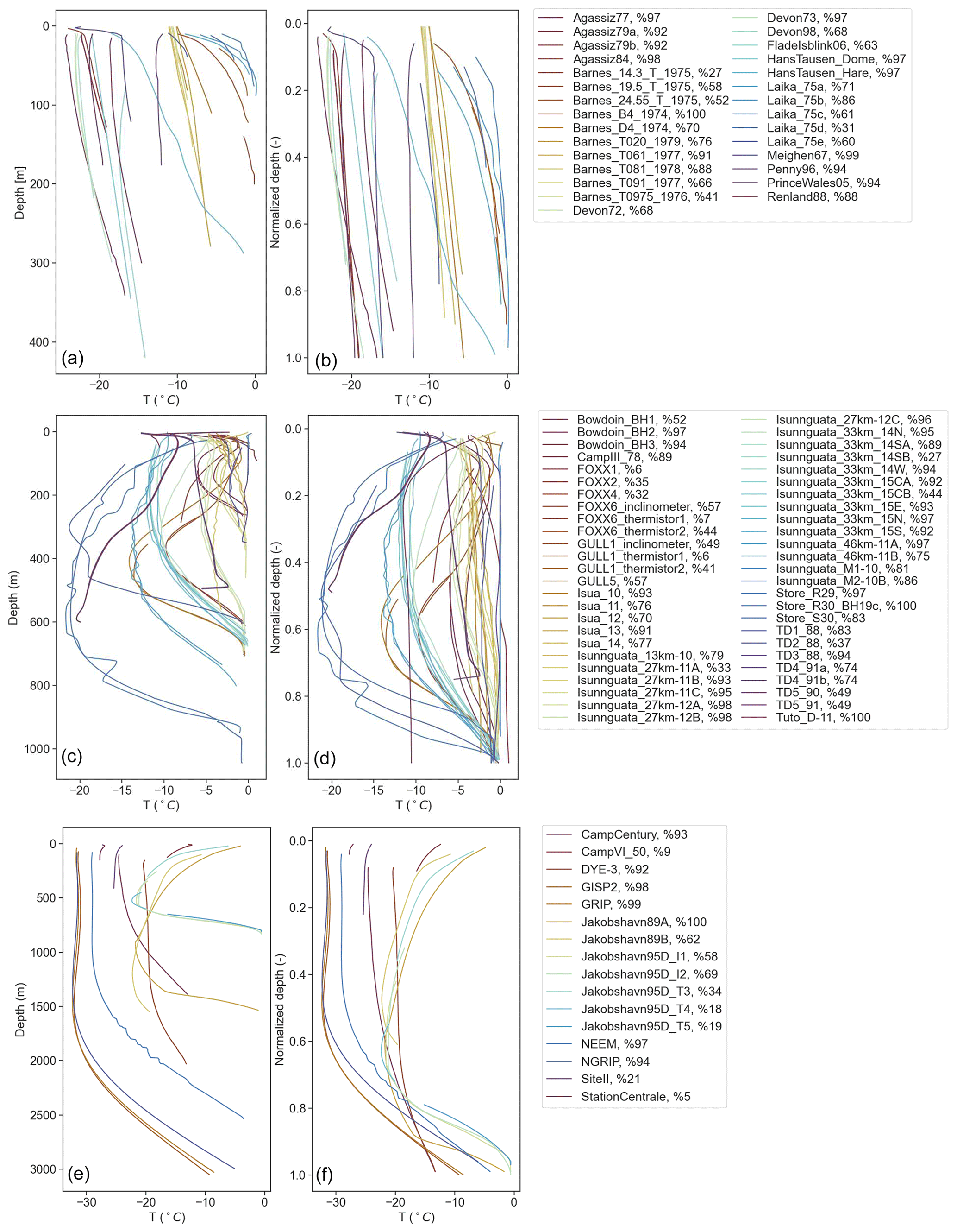
Figure 3Overview of all ice temperature profiles in the database expressed in both absolute depth (a, c, e) and normalized depth (b, c, f). For visibility, the profiles are divided into local ice caps (a, b), marginal ice sheet sites (c, d), and inland ice sheet sites (e, f). The local ice thickness coverage of each individual profile is given as a percentage.
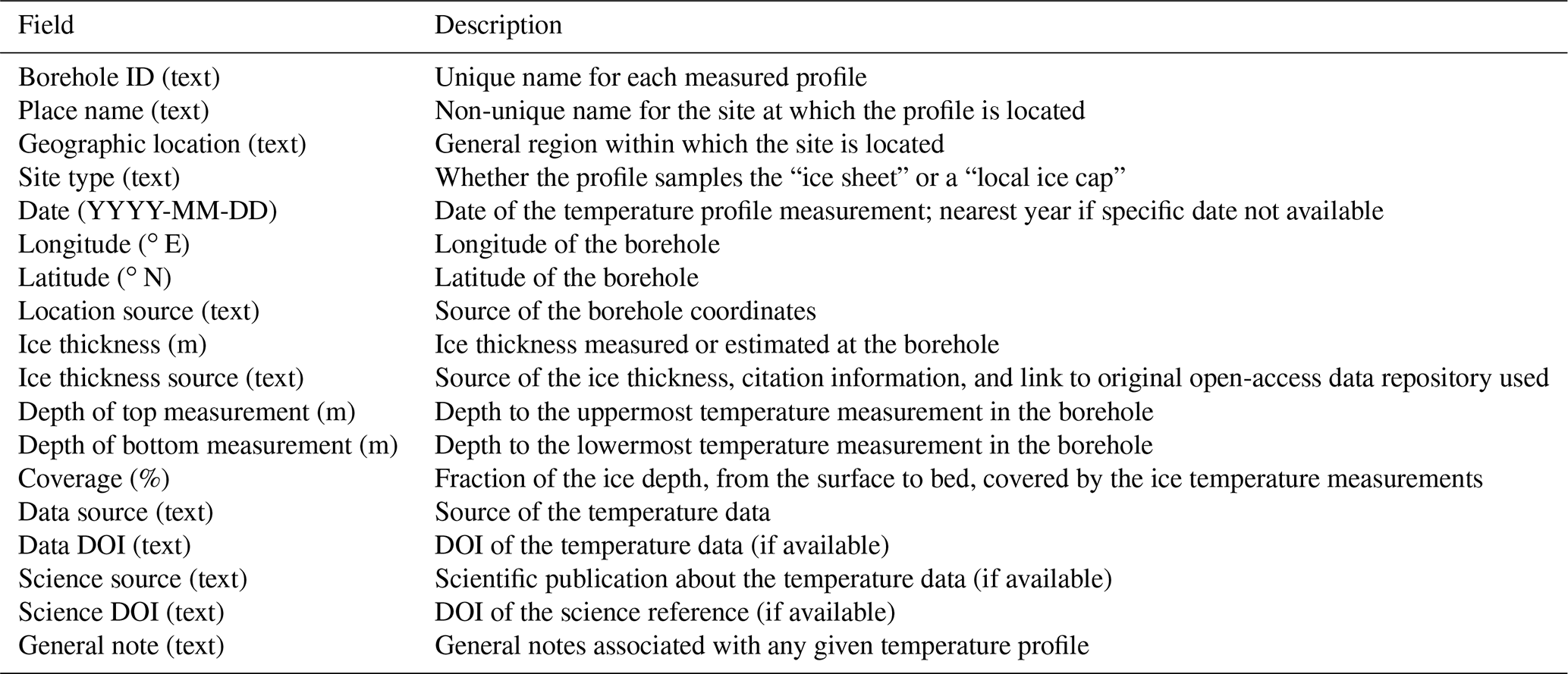
The database includes additional supplementary information. For each borehole, this information is stored in the file “meta.csv”, which contains a total of 18 metadata fields (Table 2). Every measurement entry in the database is labeled with a unique borehole ID, and a non-unique, alternative, and more descriptive place name. This alternative place name was deemed useful as, in some cases, ice temperature profiles have been measured over different campaigns by different people who have used different nomenclature for the same sites. Furthermore, borehole IDs are generally defined by either the group carrying out the measurements or by the site of the measurement. These borehole IDs are somewhat inconsistent, however, based on the differing conventions used by previously published studies.
Whenever specific locations are available, then that of each ice temperature borehole is provided in degrees east longitude and degrees north latitude. In some cases, locations have been shown in figures in the accompanying literature from which approximate locations were georeferenced. In addition to the position of the borehole, three further sets of information are provided relating to geographic setting. The site type describes whether the profile samples the Greenland ice sheet or a local ice cap. The geographic location provides a more descriptive general location of borehole sites using recognized regional geographic names. Last, the source of the location information is given.
The local ice thickness at the borehole location is provided in meters, along with the ice thickness source. When the original literature does not report the local ice thickness, an estimate is provided using BedMachine v3 (Morlighem et al., 2017). In these instances, the ice thickness is useful for determining the fraction of the ice depth, from the surface to the bed, covered by the given temperature profile and given as the percentage coverage in another field. Also listed are the depth in meters from the surface of the ice sheet to the uppermost temperature measurement of a given profile (depth of top) and the lowermost temperature measurement (depth of bottom).
For each profile, the data source describes the source of the temperature data, including links to open-access data repositories used by authors to share the original data, and the science source lists any original scientific publication that describes or mentions the temperature data. The related DOIs for both the data and science source categories are also reported when available. The date describes the common era year during which the temperature profile was measured. In the best cases, this includes the month and day that a given profile was measured. Finally, a field for additional notes is included, presenting any further information (relating to, for example, temperature, thickness, or location) that does not fit into the above categories.
Despite the best efforts of our community, there are some missing metadata fields in the database that are indicated with a question mark. The database is being continually updated. Any additional information, such as missing, updated, or new temperature data, may be added to the database by contacting the author team here or opening a GitHub issue at https://github.com/GEUS-Glaciology-and-Climate/greenland_ice_borehole_temperature_profiles/issues (last access: 1 March 2022). We use GitHub issues to resolve and identify and clarify problems in the ice temperature datasets, and we also welcome any new or missing data into the database via GitHub issues.
Of the 95 deep-ice temperature profiles making up the database, 70 originate from Greenland and 25 from the Canadian Arctic (Fig. 1). Of the 70 profiles from Greenland, 66 are from the ice sheet, and 4 are from peripheral glaciers and ice caps. All 29 peripheral glaciers and ice cap temperature profiles are plotted together in Fig. 3a and b. The peripheral glacier and ice cap profiles are relatively shallow; the deepest one reaches 420 m at a site where the ice thickness is estimated to be 520 m. Profiles from the ice sheet are divided into 50 marginal profiles (Fig. 3c and d) and 16 inland profiles (Fig. 3e and f), according to proximity to the main flow divide. The profile at GISP2, reaching bedrock at depth 3053 m and with a local ice thickness coverage of 98 %, is the deepest measurement in the database. Overall, 9 of the 95 profiles reach depths >1000 m.
The inland profiles also exhibit the coldest temperatures, with temperatures reaching a minimum of around −32 ∘C halfway down the profile at normalized depth 0.48. In total, 34 of the database's 95 profiles are from locations characterized as “cold bedded”, where the ice appears to be frozen to the bedrock. This characterization is assigned based on the observed bottom values of the profile. At some sites, we cannot speculate on the basal thermal state based on temperature observation alone. A total of eight of these cold-bedded profiles extend to >95 % of the local ice thickness (i.e., database coverage >95 %). This contrasts with 56 “warm-bedded” sites where the ice at the bed is at pressure melting point. In total, 15 of these warm-bedded profiles extend to >95 % of local ice thickness. The basal thermal state of the three sites, CampIII_78, CampVI_50, and SiteII, cannot be characterized, as these boreholes covered less than 25 % of the local ice thickness. Overall, 39 of the 95 profiles have a depth coverage >90 %.
The temporal distribution of the profiles shows how the number of available ice temperature measurements has increased over time (Fig. 4). The temperature profiles span a period of 70 years. This implies that the shallow measurement points cannot necessarily be expected to reflect current ice temperatures. Arctic air temperatures have warmed markedly during the past 7 decades. The response time for deep-ice temperature variations, however, is usually much longer than 70 years (Cuffey and Paterson, 2010). For example, at a low-accumulation site in the ice sheet interior, a surface air temperature signal from ca. 50 years ago can likely influence present-day ice temperatures at >50 m below the ice sheet surface (Muto et al., 2011; Karlsson et al., 2020).
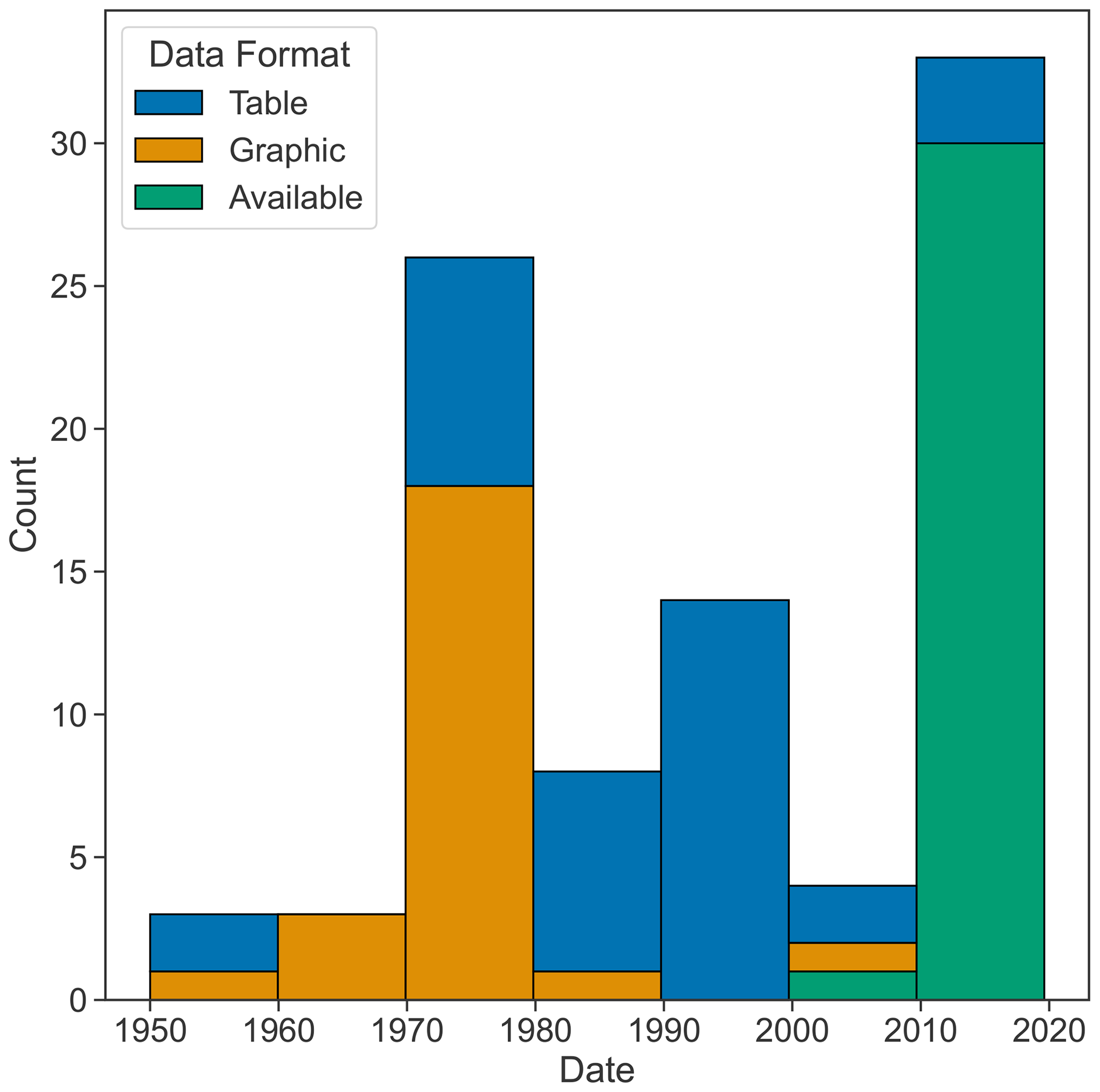
Figure 4Histogram showing the temporal distribution of the temperature profile measurements, which are color coded based on the format in which the original data were available. The profiles entered into the database were available as a digitized graphic (orange), a digitized table (blue), or already published and digitally available (green).
The majority of the ice temperature profiles presented here have not been previously available in digital format. Profiles from only 31 boreholes (ca. 36 % of the database) have been previously published in open-access data repositories (Ryser et al., 2014; Harper, 2017; Doyle et al., 2018a; Seguinot et al., 2020; Hubbard et al., 2021b; Law et al., 2021). The public availability of these profiles highlights the laudable open-science trend in the natural sciences. While we present derived products of these profiles, we provide links to the open-access repositories in which the data were originally deposited and encourage database users to recognize and cite these previous data repository sources where applicable. Profiles from 54 boreholes (ca. 64 % of the database) are made digitally available here for the first time. This includes profiles from 24 boreholes that were provided as tabulated data by community members, profiles from 24 boreholes that were digitized from previously published graphics, and 6 that were previously available as published tables.
Borehole ice temperature measurements are associated with at least three main sources of uncertainty, including measurement uncertainty, depth uncertainty, and disturbance uncertainty. There are other sources of uncertainty that we do not consider here, such as self-heating of the sensor, sensor calibration, and leakage path, to name a few (e.g., Clow et al., 1996; Clow, 2008). Measurement uncertainty reflects the accuracy with which a temperature sensor can measure ice temperature. This uncertainty is influenced by both the design and calibration of the temperature sensor. It is reasonable to suggest that the temperature sensor accuracy has improved by at least an order of magnitude from 1950 to today (from perhaps ±0.1 ∘C in the 1950s to an effective limit of better than ±0.01 ∘C today). This trend primarily reflects improvements in the down-borehole technology deployed in glaciological applications and not the absolute accuracy of temperature sensors available for public purchase.
The issue of depth uncertainty is greatest in ice temperature profiles measured by manually deployed loggers. Manual loggers can have a characteristic depth uncertainty of ±1 %. By contrast, automated winch-deployed loggers typically use rotary encoders to measure logger depth with an uncertainty better than ±0.01 %. For example, the GISP2 borehole has a drill depth of 3053 m but a logger depth of only 3050 m, which represents a discrepancy of ±0.001 % (Cuffey et al., 1995). At deep interior sites, the temperature gradient in the lower part of the ice column is typically of the order of 0.02 K m−1 (see Fig. 3e and f). At fast-moving sites, the temperature gradient may be even larger (see Fig. 3c and d), thus increasing the temperature uncertainty associated with depth uncertainty. At shallow sites, temperature gradients are typically small (see Fig. 3a and b), making the depth uncertainty negligible. For example, at Camp Century, the temperature profile was likely measured with a depth accuracy higher than ±0.1 %. With a measured basal temperature gradient of 17.5 ∘C km−1, this is equivalent to an ice temperature uncertainty of ±0.025 ∘C at the maximum borehole depth of 1388 m. There are, however, some site settings – especially when using manually deployed loggers, logging non-vertical boreholes, or measuring extreme basal temperature gradients – in which depth uncertainty can actually play a larger role in ice temperature uncertainty than temperature sensor accuracy.
Disturbance uncertainty, which is associated with ice temperatures equilibrating after drilling, is a third source of measurement uncertainty. In boreholes filled with drilling fluid, the disturbance uncertainty can include the development of convection cells within the equilibrating drilling fluid. Convection cells are expected to occur when the temperature gradient in the ice exceeds a critical value dependent on the sum of a lapse rate term and the critical potential-temperature gradient (Clow, 2014). The size and strength of convection cells is a poorly defined function of drilling fluid density, borehole diameter, and ice temperature gradient. In the Agassiz77 borehole, slight thermal instabilities in the drilling fluid produced temperature offsets of ±0.05 ∘C around the mean ice temperature gradient. In the NEEM 2011 profile, however, the convection cells between 1500 and 2000 m depth reach ca. 50 m vertical length scale and produce ±0.5 ∘C offsets around the mean ice temperature gradient (Fig. 5). The GISP-D temperature log (not presented here) also shows pronounced laminar convection cells between 1600 and 2000 m depth (Clow et al., 1996).
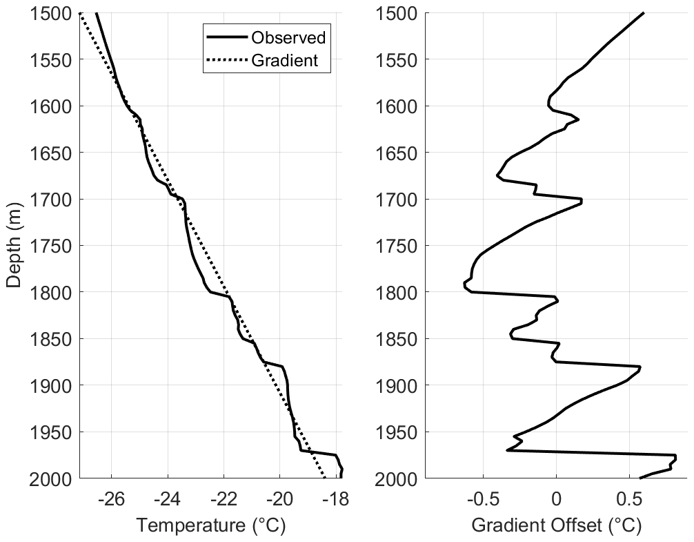
Figure 5Offsets from the mean ice temperature gradient highlight the influence of large (ca. 50 m) convection cells forming in the borehole fluid in a deep section of the NEEM ice temperature profile measured in 2011. These borehole fluid convection cells contribute to the disturbance uncertainty associated with an equilibrating borehole temperature profile when the borehole-logging technique is used. This uncertainty is avoided when sensors or cables are frozen into the ice in other measurement techniques.
Given the ultra-low density of air, air-filled boreholes cannot support analogous convection cells. The disturbance uncertainty associated with convection cells is accordingly negligible in air-filled boreholes. However, temperature disturbances due to changes in atmospheric pressure have been observed in air-filled bore holes in Antarctica. This effect is largest in the top 20 m of the borehole, just below the ice surface, with magnitudes on the order of up to ±0.003 ∘C (Clow et al., 1996). In water-filled boreholes, such as those created by hot-water drilling, the disturbance uncertainty is associated with the sensible heat released from hot drilling water and the latent heat released by borehole refreezing. This thermal disturbance of hot-water drilling often requires many months to fully dissipate, as the latent energy released by the refreezing borehole warms the surrounding ice. Empirical cooling curves of temperature measurements collected multiple times post-drilling can usually constrain this thermal disturbance effect to better than ±0.1 ∘C (Humphrey and Echelmeyer, 1990; Ryser et al., 2014; McDowell et al., 2021). Mechanically drilled ice core holes also experience thermal disturbance, resulting primarily from the sensible heat carried into the hole by the drill fluid. The associated disturbance uncertainty is, however, much smaller than for hot-water drilled holes (Clow, 2015). The temperature disturbance caused by mechanical drilling with fluid-filled boreholes dissipates to the level of precision within 5 d (Zagorodnov et al., 2012).
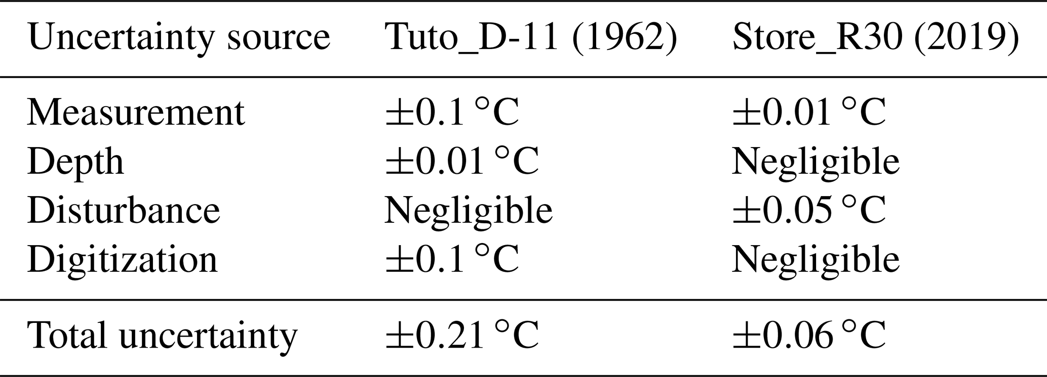
The total measurement uncertainty varies substantially between profiles in this database. Generally, these sources of uncertainty can be viewed as being independent from each other and therefore summed to estimate the total measurement uncertainty for a given ice temperature profile. Assessing this total measurement uncertainty is most critical for studies focused on absolute temperature, for example, when remeasuring present-day ice temperatures to compare with past ice temperatures at a specific site. We provide guidance for assessing the total measurement uncertainty by contrasting the uncertainty budgets of an older (Tuto_D-11; 1962) and younger (Store_R30; 2019) ice temperature profile (Table 3). The Tuto_D-11 ice temperature profile is from an air-filled borehole in which the ice temperature was measured with ca. 60-year-old sensor technology using a manually deployed logger. The Tuto_D-11 data also include an additional graphical digitization uncertainty (described in Sect. 2). The Store_R30 ice temperature profile was measured using a fiber optic string frozen into a hot-water drilled borehole that was continuously monitored to establish empirical cooling curves. The contrasting uncertainty budgets of these two boreholes (see Table 3) highlights the value of consulting the original science source publication for site-specific uncertainty assessments.
Table 3Contrasting total measurement uncertainty budgets for the Tuto_D-11 and Store_R30 ice temperature profiles. The conversion of depth uncertainty into a temperature uncertainty is done, assuming a characteristic temperature geothermal gradient of 20 ∘C km−1. Here, the word “Negligible” means that the uncertainty is <0.01 ∘C.
Numerical ice flow models are critical tools for projecting the future sea level rise contribution from the Greenland ice sheet. While the simulated initial states are typically evaluated against observed ice sheet form (i.e., thickness) and flow (i.e., velocity), the relative paucity of ice temperature data means that they are typically not evaluated against the observed ice sheet thermal state (Goelzer et al., 2020). Given the sensitivity of ice viscosity to ice temperature, biases in the thermal state of ice sheet simulations likely contribute to biases between simulated and observed recent Greenland ice loss (Goelzer et al., 2017; Aschwanden et al., 2019; Law et al., 2021). Identifying and addressing these biases in thermal state is critical for improving projections of Greenland ice loss (Aschwanden et al., 2021). To help shape a best practice for using the database that we present, we describe an approach for evaluating a contemporary ice sheet simulation against all observed Greenland deep-ice temperature observations.
Several process level studies of potential heat sources have been performed, which compare individual observed temperature profiles from local areas with temperature profiles modeled by a thermal, or thermomechanical, ice flow model (Iken et al., 1993; Lüthi et al., 2002; Harrington et al., 2015; Lüthi et al., 2015; Meierbachtol et al., 2015; McDowell et al., 2021; Law et al., 2021; Maguire et al., 2021). Although these studies featured different local areas, the comparisons generally showed that models tend to underestimate englacial temperatures and thus need to incorporate additional heat sources in order to reproduce the observed ice temperature profiles. Suggested additional heat sources include cryo-hydrological warming – which transfers latent heat when surface meltwater flows through englacial pathways and refreezes – deformational heating, and basal water heat flux (Funk et al., 1994; Wohlleben et al., 2009; Phillips et al., 2013; Lüthi et al., 2015; Zekollari et al., 2017; Karlsson et al., 2020). Modeled ice temperatures are likely also influenced by the choice of geothermal heat flow map, however, there is a diversity of opinion regarding the magnitude and spatial distribution of geothermal heat flow beneath the ice sheet (Rezvanbehbahani et al., 2017; Colgan et al., 2022).
The contemporary thermomechanical ice sheet simulation we adopt is the Parallel Ice Sheet Model (PISM; Bueler and Brown, 2009) simulation of Aschwanden et al. (2016). This simulation represents the form, flow, and thermal state of the Greenland ice sheet in ca. 1990, following a 125 kyr paleoclimatic spin-up and followed by another 2 kyr of transient equilibrium, with mass flux adjustment forcing to minimize the misfit against the observed ice sheet thickness and extent. This ice sheet simulation has a horizontal resolution of 900 m and a vertical resolution of 20 m. The geothermal heat flow map by Shapiro and Ritzwoller (2004), variable in space but not time, was used as a basal thermal boundary condition. PISM uses an enthalpy scheme for the conservation of energy calculation, in order to accommodate heat transfer in both freezing and temperate ice (Aschwanden et al., 2012). While the spin-up is meant to approximate the Greenland ice sheet at a specific time slice (ca. 1990), we are comparing this simulated thermal state with the temperature profiles observed over a 70-year time span. Shallow profiles located close to the margin can experience significant changes in ice thickness and temperature on this timescale.
At locations of observed temperature profiles, modeled vertical temperature profiles were extracted from the PISM simulation based on the nearest-neighbor grid point. Only temperature profiles from the Greenland ice sheet were included in this analysis. The PISM vertical temperature profiles were transformed from the height above bed to the normalized depth below surface and linearly interpolated to the vertical resolution of the normalized depth field of the database. Furthermore, at a few drill site locations, the modeled ice was too thin and did not have enough vertical grid points to interpolate the modeled temperatures to a proper normalized depth axis. It was therefore necessary to exclude profiles from the analysis where the simulated ice thickness was fewer than five vertical grid points (50 m). Additionally, in cases of temporally repeated observed profiles, only the most recent measurement was included in this analysis (see Table 4).
Out of the 95 temperature profiles from the temperature database, 66 were ultimately suitable for inclusion in this comparative analysis of observed and modeled ice temperatures. The observed temperature profiles were divided based on three characteristic regimes. First, whether the profiles were located in the accumulation area (16 profiles) or ablation area (38 profiles). Second, whether the basal thermal state of the profiles was considered warm bedded (44 profiles) or cold bedded (9 profiles). Finally, whether profiles were located in high-strain regions (10 profiles) or low-strain regions (46 profiles). The surface mass balance regime is determined by whether the borehole is located below the snow line, in the ablation area, or above the snow line, in the accumulation area, in contemporary satellite imagery (Fig. 1). The basal thermal state regime is based on whether the ice–bed interface is measured to be below the pressure melting point temperature (i.e., cold bedded) or not (i.e., warm bedded). In instances where the borehole does not reach the bed, we extrapolate the basal thermal state where reasonable (i.e., FladeIsblink06 is likely cold bedded), or we list the basal thermal state as being “unknown” where the extrapolation distance seems unreasonable (i.e., CampVI_50 is unknown). Finally, the ice dynamic regime is classified as being high strain when the ice flow is channelized and low strain when sites are located in sheet flow or divide flow. Figure 6 shows the observed temperature profiles for each of the three regimes.
Table 4Overview of the number of profiles in the three regimes before and after excluding profiles not usable for the model comparison analysis.
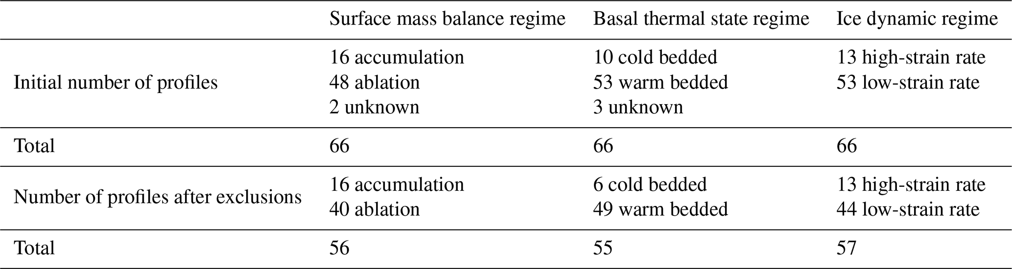
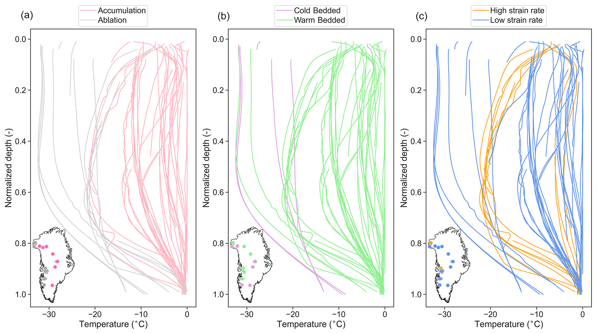
Figure 6Observed temperature profiles on a normalized depth scale for three characteristic regimes. (a) Surface mass balance regime with profiles located in the ablation area (pink) or the accumulation area (gray). (b) Basal thermal state regime with profiles either cold bedded (purple) or warm bedded (green). (c) Ice dynamic regime with profiles located either in high-strain-rate regions (orange) or low-strain-rate regions (blue).
The difference between the modeled and observed profiles was calculated at 0.01 normalized vertical resolution and then aggregated into coarser vertical layers at 0.1 normalized vertical resolution (Fig. 7). This method of examining profiles in vertical sections provides better insight to the depth variations in model bias than reducing every profile into a single metric of best fit. This vertical box plot analysis can also provide some insight with respect to which terms in the energy balance – advection, diffusion, heat production, or latent heat transfer – may be responsible for the differences between modeled and the observed profiles, as the relative importance of these terms varies with depth. Where our comparison box plots show negative temperature differences, modeled temperature values are smaller than the observed temperatures, implying that this PISM run is underestimating temperatures. The reverse occurs where box plot temperature differences are larger than 0 ∘C.
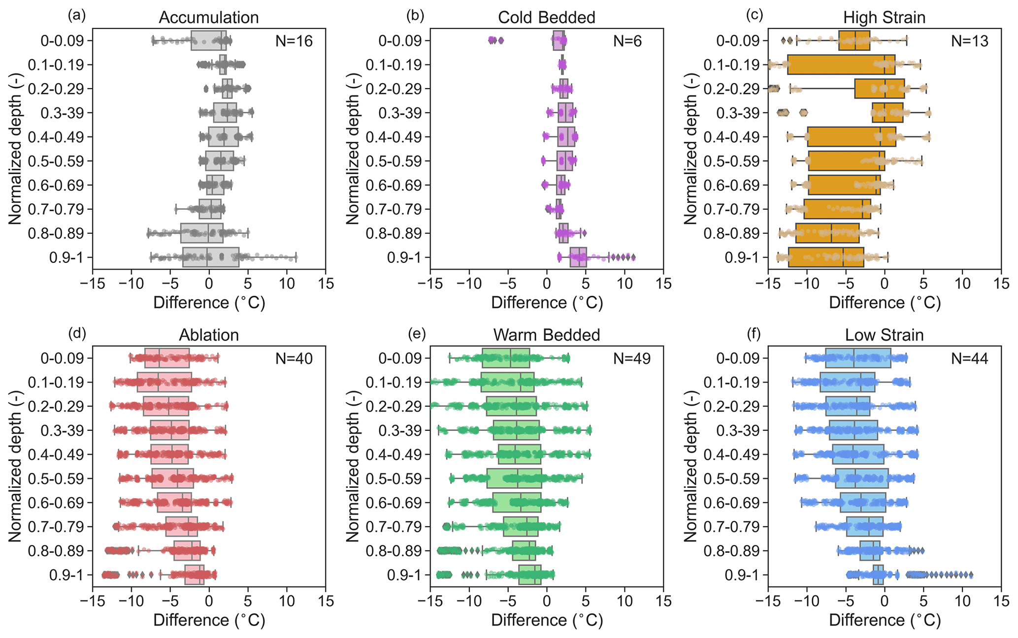
Figure 7Each plot shows the difference between the modeled minus observed normalized depth profiles aggregated into coarser vertical layers of 0.1 resolution. (a, d) Surface mass balance regime. (b, e) Basal thermal state regime. (c, f) Ice dynamic strain regime. The N value shows the number of profiles that the box plot is based on. Points plotted on top of each box plot show individual temperature difference values for all of the profiles at that depth within that category.
The surface mass balance regime comparison generally highlights a better PISM fit to observations in the accumulation area than the ablation zone (Fig. 7). This is generally expected, since the accumulation area more closely represents the theoretical steady-state temperature profiles upon which classic ice flow heat equations are predicated. The accumulation box plot shows that the mean difference value shifts from being positive in the upper part of the profile to negative, with a greater spread in differences, in the bottom 20 % of the profile. In comparison, both the ablation and temperate box plots, which share strong overlap in comprising profiles, are clearly less well captured by PISM. These warmer ablation area profiles show a larger spread in difference values throughout the entire vertical profile. Importantly, both box plots show a systematic negative mean difference at all depths, meaning that the simulation consistently underestimates ice temperatures. This may suggest that one or more heat sources are being poorly represented in warmer ablation areas in this particular PISM simulation. This is a general problem for solving the heat equation in all ice flow models. Previous studies similarly showed poor representation of the ablation area and the need to include additional heating sources to reproduce the higher observed englacial temperatures (McDowell et al., 2021).
After excluding profiles for which the modeled thickness is less than 50 m, the cold-bedded regime box plot represents the smallest sample size of just five profiles (Camp Century, Dye-3, GISP2, GRIP, and Station Central). These profiles are all drilled at inland locations where the ice is moving relatively slowly. This generally limits the role of horizontal heat advection at these sites. In contrast to the warm-bedded and ablation box plots, the cold-bedded box plot shows a systematic positive mean difference over all vertical layers, meaning that the modeled temperatures generally overestimate the observed temperatures over the entire column of ice. The largest differences between modeled and observed temperatures (+4 ∘C on average), however, are found near the ice sheet bed. Here, where vertical ice advection becomes small, the diffusion of geothermal flow should be the most influential term of the heat equation. As heat diffusion is generally well-represented and well-constrained in all ice flow models, this may suggest that this particular PISM simulation employs too high a geothermal heat flow into the ice sheet base. We note that the geothermal flow is poorly constrained under the Greenland ice sheet (Rezvanbehbahani et al., 2017; Colgan et al., 2022) and over long spin-up periods, so even small deviations in the geothermal heat flow can result in large variations in ice temperature.
The shape of temperature profiles in fast-flowing, high-strain regions is expected to have a C shape associated with strong horizontal advection of upstream ice temperatures (Cuffey and Paterson, 2010; Iken et al., 1993). While this advection of relatively cold upstream ice cools the middle depths of the ice temperature profile, in comparison to the surface boundary condition, the deformational heating warms the lower depths (Cuffey and Paterson, 2010). The high-strain box plot shows that the PISM simulation appears to systematically underestimate ice temperatures in the lowermost 50 % of the ice sheet. This bias reaches up to −5 ∘C, on average, between 80 % and 90 % depth. This underestimation of ice temperatures near the bed may result from this particular PISM simulation underestimating the strain heating associated with enhanced ice deformation in softer Last Glacial Period ice (e.g., Lüthi et al., 2002; Karlsson et al., 2013). Generally, however, it is challenging to simulate temperature profiles in high-strain ice flow regimes, as this requires correct parameterization of both local and upstream heat budgets, as well as the horizontal advection profile linking these heat budgets, in order to correctly represent steep gradients in the ice temperature profile (Cuffey and Paterson, 2010).
The low-strain box plot shows a systematic negative mean difference value across all ice depths. This suggests that, in slow-flowing regions, the model generally underestimates ice temperatures. This might be explained by this particular PISM simulation employing a spin-up surface boundary condition that had either an air temperature that is too cold or an accumulation rate that is too high. As vertical ice advection is dependent on the accumulation rate, overestimated accumulation rates can result in overestimated vertical advection rates, which enhance the advection of relatively cold near-surface ice deeper into the ice sheet. The low-strain regime profiles are diverse, however, and comprise both ablation and accumulation area profiles, with both cold and warm beds. The low-strain regime generally has the largest spread of difference values. This makes it difficult, in comparison to the other box plots presented here, to interpret a process level mechanism for the systematic cold bias across these diverse sites.
In this modeled run, the key parameters influencing the modeled temperatures are the enthalpy, which requires understanding of the liquid water fraction in the ice column and its evolution in time; the geothermal heat flow, which also has the potential to affect the presence of water in a given location; and the surface boundary conditions, i.e., accumulation rate, which control vertical temperature advection, and ice surface temperatures. These parameters are all very difficult to constrain; however, this is especially the case for the enthalpy and the geothermal heat flow parameter.
We have compiled 95 ice temperature profiles from 85 individual boreholes from Greenland and the Canadian Arctic into a comprehensive and consistent community resource. This constitutes an increase of +54 ice temperature profiles over what was previously available in open-access data repositories (64 % of the database). The scientific community is encouraged to contribute missing or new data or metadata to the database either by contacting the author team or using the GitHub issue pathway. While we expect the primary use of this database to be evaluating simulated 3-D ice temperature fields from thermomechanical ice flow models, there may soon be a sufficient number of ice temperature profiles from the Greenland ice sheet and peripheral ice caps to use machine learning approaches to spatially interpolate ice temperatures between boreholes on the basis of independent geophysical variables. This database may possibly serve as a modest first step towards addressing this emerging challenge, and other challenges, associated with understanding the thermal state of ice in Greenland and the Canadian Arctic.
We provide an initial comparison between observed ice temperature profiles and those simulated by the PISM ice flow model. This comparison highlights the inherent challenge of comparing 1-D observational datasets with an uneven spatial distribution to a simulated 3-D temperature field. These challenges include the uneven ice thickness between modeled and observed geometry, especially at marginal sites; resolving the difference between the systematic biases and random error in the modeled temperature profiles; and confronting the fundamental uncertainty in the basal thermal state due to complex processes. In this comparison, the poor representation of cryo-hydrological warming, or the transfer of latent energy, appears to be contributing to a model cold bias at peripheral ice sheet sites. Similarly, the poor representation of deformational heating and vertical ice stratigraphy appears to be contributing to a model cold bias at high-strain-rate sites. Clearly, thermomechanical models provide the most reliable solution to the heat equation in low-strain, cold-bedded inland areas.
The Greenland deep-ice temperature database described here is available at https://doi.org/10.22008/FK2/3BVF9V (Mankoff et al., 2022). The source or inputs to the database are available at https://github.com/GEUS-PROMICE/greenland_ice_borehole_temperature_profiles (last access: 3 March 2022; Mankoff, 2022). The supplementary metadata described in this article, including profile classification, are available in the Supplement.
Users of this product should cite the data repository (Mankoff et al., 2022) and this descriptive data article. Users of this product should also cite the original “Data Source” and “Data DOI” repositories when they are available. We encourage data users to similarly consult the relevant “Science Source” articles, which can be found in the metadata for each profile. Furthermore, data users who are generating derivative products from database entries are requested to invite collaboration with the “Science Source” team associated with the database entries being utilized.
The supplement related to this article is available online at: https://doi.org/10.5194/tc-17-3829-2023-supplement.
Conceptualization by WTC and KDM; data curation by WTC, KDM, HHT, GDC, DF, CZ, MPL, BMV, DDJ, IM, HZ, TM, SHD, AA, BeH, RL, JH, NH, BrH, PC, MJ, and JS; formal analysis by AL, SHD, AA, RL, and JH; funding acquisition by JH, BrH, and PC; investigation by AL, SHD, AA, RL, JH, BrH, and PC; interpretation by AL, AS, HHT, GDC, MPL, NBK, HZ, SHD, RL, JH, BrH, and PC; methodology by AL, KDM, WTC, GDC, NBK, RL, JH, BrH, and PC; project administration by KDM, WTC, RSF, SAK, JH, BrH, and PC; resources by RSF and SAK; software by KDM; supervision by KDM, WTC, JH, BrH, and PC; validation by AL, KDM, WTC, AS, NBK, and SHD; visualization by AL and KDM; and pre-submission writing by AL, KDM, WTC, GDC, NBK, HZ, SHD, RL, BrH, and PC.
At least one of the (co-)authors is a member of the editorial board of The Cryosphere. The peer-review process was guided by an independent editor, and the authors also have no other competing interests to declare.
Publisher's note: Copernicus Publications remains neutral with regard to jurisdictional claims in published maps and institutional affiliations.
We thank Baptiste Vandercrux and Joseph A. MacGregor for their discussion during the development of this database. We also note that Fig. 2 is reprinted from the Journal of Glaciology, with the permission of the International Glaciological Society. We thank Brice Van Liefferinge (Université Libre de Bruxelles) and one anonymous reviewer for providing insightful feedback on this work. We also thank Carlos Martin (British Antarctic Survey) for serving as the scientific reviewer for this paper.
The development of this database by the Geological Survey of Denmark and Greenland (GEUS) has been supported by the Programme for Monitoring of the Greenland Ice Sheet (http://www.promice.dk, last access: 4 September 2023), the Independent Research Fund Denmark award (IRFD; grant no. 8049-00003B), and a Villum Foundation award (grant no. 00022885). Ice coring on the Canadian Arctic ice caps has been primarily supported by the Polar Continental Shelf Project and the Geological Survey of Canada (Natural Resources Canada), with additional funding from the Canadian Foundation for Climate and Atmospheric Science (Prince of Wales Icefield 2005) and Japan's Science and Technology Agency (Penny Ice Cap, 1996). Harry Zekollari received funding from the Fonds de la Recherche Scientifique – FNRS (postdoctoral grant – chargé de recherches) and PROTECT, which has received funding from the European Union's Horizon 2020 research and innovation programme (grant no. 869304). Ice temperature measurements on Store Glacier have been supported by the European Union's Horizon 2020 research and innovation programme (grant no. 683048; RESPONDER), the National Environment Research Council (NERC; SAFIRE grant nos. NE/K006126 and NE/K005871/1), and an Aberystwyth University Capital Equipment grant. Andy Aschwanden has been supported by NASA (grant no. 20-CRYO2020-0052). Robert Law received funding from a NERC Doctoral Training Partnership studentship (grant no. NE/L002507/1). Mylène Jacquemart received funding from the Swiss National Science Foundation (grant no. SNSF 184634; PROGGRESS). Joel Harper, Neil Humphrey, Toby Meierbachtol, Ian McDowell, and Benjamin Hills have been funded by the U.S. National Science Foundation, Office of Polar Programs (grant nos. 1203451 and 0909495). Gary D. Clow received funding from the U.S. Geological Survey and the U.S. National Science Foundation, Office of Polar Programs. Martin P. Lüthi received funding from the Swiss National Science Foundation (grant no. 200021-127197). Julien Seguinot received funding from the Swiss National Science Foundation (SNSF; grant nos. 200020-169558 and 200021-153179/1) to Martin Funk (ETHZ) and the Trond Mohn Stiftelse (TMS) and University of Bergen (UiB) start-up (grant no. TMS2022STG03) to Suzette Flantua (UiB).
This paper was edited by Carlos Martin and reviewed by Brice Van Liefferinge and one anonymous referee.
Aschwanden, A., Bueler, E., Khroulev, C., and Blatter, H.: An enthalpy formulation for glaciers and ice sheets, J. Glaciol., 58, 441–457, https://doi.org/10.3189/2012JoG11J088, 2012. a
Aschwanden, A., Fahnestock, M. A., and Truffer, M.: Complex Greenland outlet glacier flow captured, Nat. Commun., 7, 1–8, https://doi.org/10.1038/ncomms10524, 2016. a
Aschwanden, A., Fahnestock, M. A., Truffer, M., Brinkerhoff, D. J., Hock, R., Khroulev, C., Mottram, R., and Khan, S. A.: Contribution of the Greenland Ice Sheet to sea level over the next millennium, Sci. Adv., 5, eaav9396, https://doi.org/10.1126/sciadv.aav9396, 2019. a, b
Aschwanden, A., Bartholomaus, T. C., Brinkerhoff, D. J., and Truffer, M.: Brief communication: A roadmap towards credible projections of ice sheet contribution to sea level, The Cryosphere, 15, 5705–5715, https://doi.org/10.5194/tc-15-5705-2021, 2021. a, b
Bindschadler, R. A., Nowicki, S., Abe-Ouchi, A., Aschwanden, A., Choi, H., Fastook, J., Granzow, G., Greve, R., Gutowski, G., Herzfeld, U., Jackson, C., Johnson, J., Khroulev, C., Levermann, A., Lipscomb, W. H., Martin, M. A., Morlighem, M., Parizek, B. R., Pollard, D., Price, S. F., Ren, D., Saito, F., Sato, T., Seddik, H., Seroussi, H., Takahashi, K., Walker, R., and Wang, W. L.: Ice-sheet model sensitivities to environmental forcing and their use in projecting future sea level (the SeaRISE project), J. Glaciol., 59, 195–224, https://doi.org/10.3189/2013JoG12J125, 2013. a
Blatter, H. and Kappenberger, G.: Mass balance and thermal regime of Laika ice cap, Coburg Island, NWT, Canada, J. Glaciol., 34, 102–110, 1988. a
Buchardt, S. L. and Dahl-Jensen, D.: Estimating the basal melt rate at NorthGRIP using a Monte Carlo technique, Ann. Glaciol., 45, 137–142, https://doi.org/10.3189/172756407782282435, 2007. a
Bueler, E. and Brown, J.: Shallow shelf approximation as a “sliding law” in a thermodynamically coupled ice sheet model, J. Geophys. Res., 114, F03008, https://doi.org/10.1029/2008JF001179, 2009. a
Calov, R. and Hutter, K.: The thermomechanical response of the Greenland Ice Sheet to various climate scenarios, Clim. Dynam., 12, 243–260, https://doi.org/10.1007/BF00219499, 1996. a
Clarke, G. K., Fisher, D. A., and Waddington, E. D.: Wind pumping: a potentially significant heat source in ice sheets, International Association of Hydrological Sciences Publication, 170, 169–180, 1987. a
Classen, D.: Temperature profiles for the Barnes Ice Cap surge zone, J. Glaciol., 18, 391–405, 1977. a, b
Clow, G.: A Green's function approach for assessing the thermal disturbance caused by drilling deep boreholes in rock or ice, Geophys. J. Int., 203, 1877–1895, https://doi.org/10.1093/gji/ggv415, 2015. a
Clow, G. D.: USGS polar temperature logging system, description and measurement uncertainties, Tech. rep., US Department of the Interior, US Geological Survey, https://doi.org/10.3133/tm2E3, 2008. a, b
Clow, G. D.: Temperature data acquired from the DOI/GTN-P Deep Borehole Array on the Arctic Slope of Alaska, 1973–2013, Earth Syst. Sci. Data, 6, 201–218, https://doi.org/10.5194/essd-6-201-2014, 2014. a
Clow, G. D., Saltus, R. W., and Waddington, E. D.: A new high-precision borehole-temperature logging system used at GISP2, Greenland, and Taylor Dome, Antarctica, J. Glaciol., 42, 576–584, 1996. a, b, c
Colbeck, S. and Gow, A.: The margin of the Greenland Ice Sheet at ISUA, J. Glaciol., 24, 155–165, 1979. a
Colgan, W., Sommers, A., Rajaram, H., Abdalati, W., and Frahm, J.: Considering thermal-viscous collapse of the Greenland Ice Sheet, Earth's Future, 3, 252–267, https://doi.org/10.1002/2015EF000301, 2015. a
Colgan, W., Wansing, A., Mankoff, K., Lösing, M., Hopper, J., Louden, K., Ebbing, J., Christiansen, F. G., Ingeman-Nielsen, T., Liljedahl, L. C., MacGregor, J. A., Hjartarson, Á., Bernstein, S., Karlsson, N. B., Fuchs, S., Hartikainen, J., Liakka, J., Fausto, R. S., Dahl-Jensen, D., Bjørk, A., Naslund, J.-O., Mørk, F., Martos, Y., Balling, N., Funck, T., Kjeldsen, K. K., Petersen, D., Gregersen, U., Dam, G., Nielsen, T., Khan, S. A., and Løkkegaard, A.: Greenland Geothermal Heat Flow Database and Map (Version 1), Earth Syst. Sci. Data, 14, 2209–2238, https://doi.org/10.5194/essd-14-2209-2022, 2022. a, b
Cuffey, K. M. and Clow, G. D.: Temperature, accumulation, and ice sheet elevation in central Greenland through the last deglacial transition, J. Geophys. Res.-Oceans, 102, 26383–26396, https://doi.org/10.1029/96JC03981, 1997. a
Cuffey, K. M. and Paterson, W. S. B.: The physics of glaciers, Academic Press, ISBN 978-0123694614, 2010. a, b, c, d, e
Cuffey, K. M., Clow, G. D., Alley, R. B., Stuiver, M., Waddington, E. D., and Saltus, R. W.: Large arctic temperature change at the Wisconsin-Holocene glacial transition, Science, 270, 455–458, 1995. a, b
Dahl-Jensen, D., Mosegaard, K., Gundestrup, N., Clow, G. D., Johnsen, S. J., Hansen, A. W., and Balling, N.: Past temperatures directly from the Greenland Ice Sheet, Science, 282, 268–271, 1998. a
Davis, R.: Approach roads, Greenland 1960–1964, Tech. rep., Cold Regions Research and Engineering Lab Hanover NH, https://apps.dtic.mil/sti/citations/AD0726914 (last access: 4 September 2023), 1967. a, b, c
Doyle, S., Hubbard, B., Christoffersen, P., Young, T. J., Hofstede, C., Bougamont, M., Box, J., and Hubbard, A.: SAFIRE borehole, AWS and GPS datasets (Version 1), figshare [data set], https://doi.org/10.6084/m9.figshare.5745294.v1, 2018a. a
Doyle, S. H., Hubbard, B., Christoffersen, P., Young, T. J., Hofstede, C., Bougamont, M., Box, J., and Hubbard, A.: Physical conditions of fast glacier flow: 1. Measurements from boreholes drilled to the bed of Store Glacier, West Greenland, J. Geophys. Res.-Earth Surf., 123, 324–348, https://doi.org/10.1002/2017JF004529, 2018b. a
Fischer, H., Werner, M., Wagenbach, D., Schwager, M., Thorsteinnson, T., Wilhelms, F., Kipfstuhl, J., and Sommer, S.: Little ice age clearly recorded in northern Greenland ice cores, Geophys. Res. Lett., 25, 1749–1752, https://doi.org/10.1029/98GL01177, 1998. a
Funk, M., Echelmeyer, K., and Iken, A.: Mechanisms of fast flow in Jakobshavns Isbræ, West Greenland: Part II. Modeling of englacial temperatures, J. Glaciol., 40, 569–585, 1994. a, b
Goelzer, H., Robinson, A., Seroussi, H., and Van De Wal, R. S.: Recent progress in Greenland Ice Sheet modelling, Current climate change reports, 3, 291–302, https://doi.org/10.1007/s40641-017-0073-y, 2017. a
Goelzer, H., Nowicki, S., Payne, A., Larour, E., Seroussi, H., Lipscomb, W. H., Gregory, J., Abe-Ouchi, A., Shepherd, A., Simon, E., Agosta, C., Alexander, P., Aschwanden, A., Barthel, A., Calov, R., Chambers, C., Choi, Y., Cuzzone, J., Dumas, C., Edwards, T., Felikson, D., Fettweis, X., Golledge, N. R., Greve, R., Humbert, A., Huybrechts, P., Le clec'h, S., Lee, V., Leguy, G., Little, C., Lowry, D. P., Morlighem, M., Nias, I., Quiquet, A., Rückamp, M., Schlegel, N.-J., Slater, D. A., Smith, R. S., Straneo, F., Tarasov, L., van de Wal, R., and van den Broeke, M.: The future sea-level contribution of the Greenland ice sheet: a multi-model ensemble study of ISMIP6, The Cryosphere, 14, 3071–3096, https://doi.org/10.5194/tc-14-3071-2020, 2020. a, b
Gowan, E. J., Zhang, X., Khosravi, S., Rovere, A., Stocchi, P., Hughes, A. L., Gyllencreutz, R., Mangerud, J., Svendsen, J.-I., and Lohmann, G.: A new global ice sheet reconstruction for the past 80 000 years, Nat. Commun., 12, 1–9, https://doi.org/10.1038/s41467-021-21469-w, 2021. a
Gundestrup, N. and Hansen, B. L.: Bore-hole survey at Dye 3, south Greenland, J. Glaciol., 30, 282–288, 1984. a, b, c
Gundestrup, N., Dahl-Jensen, D., Hansen, B., and Kelty, J.: Bore-hole survey at Camp Century, 1989, Cold Reg. Sci. Technol., 21, 187–193, 1993. a
Hansen, B. and Landauer, J.: Some results of ice cap drill hole measurements, IASH Publ., 47, 313–317, 1958. a
Hansson, M. E.: The Renland ice core. A northern hemisphere record of aerosol composition over 120,000 years, Tellus B, 46, 390–418, 1994. a
Harper, J.: Ice temperatures measured in a grid of boreholes, Western Greenland, 2014–2016, Arctic Data Center [data set], https://doi.org/10.18739/A24746S04, 2017. a
Harper, J. and Meierbachtol, T.: Western Greenland Ice Sheet ice temperature profiles, 2010–2012, Arctic Data Center [data set], https://doi.org/10.18739/A2QV3C51Q, 2021. a
Harrington, J. A., Humphrey, N. F., and Harper, J. T.: Temperature distribution and thermal anomalies along a flowline of the Greenland ice sheet, Ann. Glaciol., 56, 98–104, https://doi.org/10.3189/2015AoG70A945, 2015. a, b
Heuberger, J. C.: Expéditions Polaires Françaises: Missions Paul-Emil Victor. Glaciologie Groenland Volume 1: Forages sur l'inlandsis, Tech. Rep. 1214, 1954. a, b
Hills, B. H., Harper, J. T., Humphrey, N. F., and Meierbachtol, T. W.: Measured horizontal temperature gradients constrain heat transfer mechanisms in Greenland ice, Geophys. Res. Lett., 44, 9778–9785, https://doi.org/10.1002/2017GL074917, 2017. a
Hubbard, B., Christoffersen, P., Doyle, S. H., Chudley, T. R., Schoonman, C. M., Law, R., and Bougamont, M.: Borehole-based characterization of ceep mixed-mode crevasses at a Greenlandic outlet glacier, AGU Adv., 2, e2020AV000291, https://doi.org/10.1029/2020AV000291, 2021a. a
Hubbard, B., Christoffersen, P., Doyle, S. H., Chudley, T. R., Schoonman, C. M., Law, R., and Bougamont, M.: Supporting data for “Borehole-based characterization of deep crevasses at a Greenlandic outlet glacier” published in AGU Advances, figshare [data set], https://doi.org/10.6084/m9.figshare.13400072.v2, 2021b. a
Humphrey, N. and Echelmeyer, K.: Hot-water drilling and bore-hole closure in cold ice, J. Glaciol., 36, 287–298, https://doi.org/10.3189/002214390793701354, 1990. a
Huybrechts, P., Letreguilly, A., and Reeh, N.: The Greenland ice sheet and greenhouse warming, Palaeogeogr. Palaeoclimatol., 89, 399–412, https://doi.org/10.1016/0031-0182(91)90174-P, 1991. a
Iken, A., Echelmeyer, K., Harrison, W., and Funk, M.: Mechanisms of fast flow in Jakobshavns Isbræ, West Greenland: Part I. Measurements of temperature and water level in deep boreholes, J. Glaciol., 39, 15–25, https://doi.org/10.3189/S0022143000015689, 1993. a, b, c, d
Jezek, K. C., Yardim, C., Johnson, J. T., Macelloni, G., and Brogioni, M.: Analysis of ice-sheet temperature profiles from low-frequency airborne remote sensing, J. Glaciol., 68, 1–11, https://doi.org/10.1017/jog.2022.19, 2022. a
Johnsen, S. J., Dahl-Jensen, D., Dansgaard, W., and Gundestrup, N.: Greenland palaeotemperatures derived from GRIP bore hole temperature and ice core isotope profiles, Tellus B, 47, 624–629, https://doi.org/10.3402/tellusb.v47i5.16077, 1995. a
Karlsson, N. B., Dahl-Jensen, D., Prasad Gogineni, S., and Paden, J. D.: Tracing the depth of the Holocene ice in North Greenland from radio-echo sounding data, Ann. Glaciol., 54, 44–50, https://doi.org/10.3189/2013AoG64A057, 2013. a
Karlsson, N. B., Razik, S., Hörhold, M., Winter, A., Steinhage, D., Binder, T., and Eisen, O.: Surface accumulation in Northern Central Greenland during the last 300 years, Ann. Glaciol., 61, 214–224, https://doi.org/10.1017/aog.2020.30, 2020. a, b
Kinnard, C., Zdanowicz, C. M., Fisher, D. A., and Wake, C. P.: Calibration of an ice-core glaciochemical (sea-salt) record with sea-ice variability in the Canadian Arctic, Ann. Glaciol., 44, 383–390, https://doi.org/10.3189/172756406781811349, 2006. a
Kinnard, C., Koerner, R. M., Zdanowicz, C. M., Fisher, D. A., Zheng, J., Sharp, M. J., Nicholson, L., and Lauriol, B.: Stratigraphic analysis of an ice core from the Prince of Wales Icefield, Ellesmere Island, Arctic Canada, using digital image analysis: High-resolution density, past summer warmth reconstruction, and melt effect on ice core solid conductivity, J. Geophys. Res.-Atmos., 113, D24120, https://doi.org/10.1029/2008JD011083, 2008. a
Law, R., Christoffersen, P., Hubbard, B., Doyle, S. H., Chudley, T. R., Schoonman, C. M., Bougamont, M., des Tombe, B., Schilperoort, B., Kechavarzi, C., Booth, A., and Young, T. J.: Thermodynamics of a fast-moving Greenlandic outlet glacier revealed by fiber-optic distributed temperature sensing, Sci. Adv., 7, eabe7136, https://doi.org/10.1126/sciadv.abe7136, 2021. a, b, c, d, e
Lemark, A. and Dahl-Jensen, D.: A study of the Flade Isblink ice cap using a simple ice flow model, Master's thesis, Niels Bohr Institute, Copenhagen University, 2010. a
Letréguilly, A., Reeh, N., and Huybrechts, P.: The Greenland ice sheet through the last glacial-interglacial cycle, Palaeogeogr. Palaeocl., 90, 385–394, https://doi.org/10.1016/S0031-0182(12)80037-X, 1991. a
Lüthi, M., Funk, M., Iken, A., Gogineni, S., and Truffer, M.: Mechanisms of fast flow in Jakobshavn Isbræ, West Greenland: Part III. Measurements of ice deformation, temperature and cross-borehole conductivity in boreholes to the bedrock, J. Glaciol., 48, 369–385, https://doi.org/10.3189/172756502781831322, 2002. a, b, c, d
Lüthi, M. P., Ryser, C., Andrews, L. C., Catania, G. A., Funk, M., Hawley, R. L., Hoffman, M. J., and Neumann, T. A.: Heat sources within the Greenland Ice Sheet: dissipation, temperate paleo-firn and cryo-hydrologic warming, The Cryosphere, 9, 245–253, https://doi.org/10.5194/tc-9-245-2015, 2015. a, b
Macelloni, G., Leduc-Leballeur, M., Montomoli, F., Brogioni, M., Ritz, C., and Picard, G.: On the retrieval of internal temperature of Antarctica Ice Sheet by using SMOS observations, Remote Sens. Environ., 233, 111405, https://doi.org/10.1016/j.rse.2019.111405, 2019. a
MacGregor, J. A., Fahnestock, M. A., Catania, G. A., Aschwanden, A., Clow, G. D., Colgan, W. T., Gogineni, S. P., Morlighem, M., Nowicki, S. M., Paden, J. D., Price, S. F., and Seroussi, H.: A synthesis of the basal thermal state of the Greenland Ice Sheet, J. Geophys. Res.-Earth Surf., 121, 1328–1350, https://doi.org/10.1002/2015JF003803, 2016. a
MacGregor, J. A., Fahnestock, M. A., Colgan, W. T., Larsen, N. K., Kjeldsen, K. K., and Welker, J. M.: The age of surface-exposed ice along the northern margin of the Greenland Ice Sheet, J. Glaciol., 66, 667–684, https://doi.org/10.1017/jog.2020.62, 2020. a
MacGregor, J. A., Chu, W., Colgan, W. T., Fahnestock, M. A., Felikson, D., Karlsson, N. B., Nowicki, S. M. J., and Studinger, M.: GBaTSv2: a revised synthesis of the likely basal thermal state of the Greenland Ice Sheet, The Cryosphere, 16, 3033–3049, https://doi.org/10.5194/tc-16-3033-2022, 2022. a
Machguth, H., Thomsen, H. H., Weidick, A., Ahlstrøm, A. P., Abermann, J., Andersen, M. L., Andersen, S. B., Bjørk, A. A., Box, J. E., Braithwaite, R. J., Bøggild, C. E., Citterio, M., Clement, P., Colgan, W., Fausto, R. F., Gleie, K., Gubler, S., Hasholt, B., Hynek, B., Knudsen, N. T., Larsen, S. H., Mernild, S. H., Oerlemans, J., Oerter, H., Olesen, O. B., Smeets, C. J. P. P., Steffen, K., Stober, M., Sugiyama, S., van As, D., van den Broeke, M. R., and van de Wal, R. S.: Greenland surface mass-balance observations from the ice-sheet ablation area and local glaciers, J. Glaciol., 62, 861–887, https://doi.org/10.1017/jog.2016.75, 2016. a
Maguire, R., Schmerr, N., Pettit, E., Riverman, K., Gardner, C., DellaGiustina, D. N., Avenson, B., Wagner, N., Marusiak, A. G., Habib, N., Broadbeck, J. I., Bray, V. J., and Bailey, S. H.: Geophysical constraints on the properties of a subglacial lake in northwest Greenland, The Cryosphere, 15, 3279–3291, https://doi.org/10.5194/tc-15-3279-2021, 2021. a
Mankoff, K. D.: Greenland deep ice temperature database, github, https://github.com/GEUS-Glaciology-and-Climate/greenland_ice_borehole_temperature_profiles (last access: 4 September 2023), 2022. a, b, c, d
Mankoff, K., Løkkegaard, A., Colgan, W., Thomsen, H., Clow, G., Fisher, D., Zdanowicz, C., Lüthi, M. P., Vinther, B., MacGregor, J. A., McDowell, I., Zekollari, H., Meierbachtol, T., Doyle, S., Law, R., Hills, B., Harper, J., Humphrey, N., Hubbard, B., Christoffersen, P., and Jacquemart, M.: Greenland deep ice temperature database, V1, GEUS Dataverse [data set], https://doi.org/10.22008/FK2/3BVF9V, 2022. a, b, c, d
McDowell, I. E., Humphrey, N. F., Harper, J. T., and Meierbachtol, T. W.: The cooling signature of basal crevasses in a hard-bedded region of the Greenland Ice Sheet, The Cryosphere, 15, 897–907, https://doi.org/10.5194/tc-15-897-2021, 2021. a, b, c
Meierbachtol, T. W., Harper, J. T., Johnson, J. V., Humphrey, N. F., and Brinkerhoff, D. J.: Thermal boundary conditions on western Greenland: Observational constraints and impacts on the modeled thermomechanical state, J. Geophys. Res.-Earth Surf., 120, 623–636, https://doi.org/10.1002/2014JF003375, 2015. a
Moon, T., Fisher, M., Harden, L., and Stafford, T.: QGreenland (v1. 0.1), Zenodo [software], https://doi.org/10.5281/zenodo.4558266, 2021. a
Morlighem, M., Williams, C. N., Rignot, E., An, L., Arndt, J. E., Bamber, J. L., Catania, G., Chauché, N., Dowdeswell, J. A., Dorschel, B., Fenty, I., Hogan, K., Howat, I., Hubbard, A., Jakobsson, M., Jordan, T. M., Kjeldsen, K. K., Millan, R., Mayer, L., Mouginot, J., Noël, B. P. Y., O'Cofaigh, C., Palmer, S., Rysgaard, S., Seroussi, H., Siegert, M. J., Slabon, P., Straneo, F., van den Broeke, M. R., Weinrebe, W., Wood, M., and Zinglersen, K. B.: BedMachine v3: Complete bed topography and ocean bathymetry mapping of Greenland from multibeam echo sounding combined with mass conservation, Geophys. Res. Lett., 44, 11051–11061, https://doi.org/10.1002/2017GL074954, 2017. a
Muto, A., Scambos, T. A., Steffen, K., Slater, A. G., and Clow, G. D.: Recent surface temperature trends in the interior of East Antarctica from borehole firn temperature measurements and geophysical inverse methods, Geophys. Res. Lett., 38, L15502, https://doi.org/10.1029/2011GL048086, 2011. a
Paterson, W.: A temperature profile through the Meighen ice cap, Arctic Canada, International Association of Scientific Hydrology, Publication, 79, 440–449, 1968. a
Paterson, W., Koerner, R., Fisher, D., Johnsen, S., Clausen, H., Dansgaard, W., Bucher, P., and Oeschger, H.: An oxygen-isotope climatic record from the Devon Island ice cap, arctic Canada, Nature, 266, 508–511, 1977. a
Phillips, T., Rajaram, H., Colgan, W., Steffen, K., and Abdalati, W.: Evaluation of cryo-hydrologic warming as an explanation for increased ice velocities in the wet snow zone, Sermeq Avannarleq, West Greenland, J. Geophys. Res.-Earth Surf., 118, 1241–1256, https://doi.org/10.1002/jgrf.20079, 2013. a
Rasmussen, S. O., Abbott, P. M., Blunier, T., Bourne, A. J., Brook, E., Buchardt, S. L., Buizert, C., Chappellaz, J., Clausen, H. B., Cook, E., Dahl-Jensen, D., Davies, S. M., Guillevic, M., Kipfstuhl, S., Laepple, T., Seierstad, I. K., Severinghaus, J. P., Steffensen, J. P., Stowasser, C., Svensson, A., Vallelonga, P., Vinther, B. M., Wilhelms, F., and Winstrup, M.: A first chronology for the North Greenland Eemian Ice Drilling (NEEM) ice core, Clim. Past, 9, 2713–2730, https://doi.org/10.5194/cp-9-2713-2013, 2013. a
Rezvanbehbahani, S., Stearns, L. A., Kadivar, A., Walker, J. D., and van der Veen, C. J.: Predicting the Geothermal Heat Flux in Greenland: A Machine Learning Approach, Geophys. Res. Lett., 44, 12271–12279, https://doi.org/10.1002/2017GL075661, 2017. a, b
Rohatgi, A.: Webplotdigitizer: Version 4.5, https://automeris.io/WebPlotDigitizer (last access: 4 September 2023), 2021. a
Ryser, C., Lüthi, M. P., Andrews, L. C., Hoffman, M. J., Catania, G. A., Hawley, R. L., Neumann, T. A., and Kristensen, S. S.: Sustained high basal motion of the Greenland ice sheet revealed by borehole deformation, J. Glaciol., 60, 647–660, https://doi.org/10.3189/2014JoG13J196, 2014. a, b, c, d, e
Seguinot, J., Funk, M., Bauder, A., Wyder, T., Senn, C., and Sugiyama, S.: Englacial warming indicates deep crevassing in Bowdoin glacier, Greenland, Front. Earth Sci., 8, 65, https://doi.org/10.3389/feart.2020.00065, 2020. a, b
Shapiro, N. M. and Ritzwoller, M. H.: Inferring surface heat flux distributions guided by a global seismic model: particular application to Antarctica, Earth Planet. Sc. Lett., 223, 213–224, https://doi.org/10.1016/j.epsl.2004.04.011, 2004. a
Stauffer, B. and Oeschger, H.: Temperaturprofile in Bohrlöchern am Rande des grönländischen Inlandeises, Eidg. Tech. Hochschule, Zurich Versuchsanst. Wasserbau, Hydrol. Glaziol. Mill, 41, 301–313, 1979. a
Tarasov, L. and Peltier, W.: A geophysically constrained large ensemble analysis of the deglacial history of the North American ice-sheet complex, Quaternary Sci. Rev., 23, 359–388, https://doi.org/10.1016/j.quascirev.2003.08.004, 2004. a
Thomsen, H., Olesen, O. B., Braithwaite, R. J., and Bøggild, C. E.: Ice drilling and mass balance at Pâkitsoq, Jakobshavn, central West Greenland, Rapport Grønlands Geologiske Undersøgelse, 152, 80–84, https://doi.org/10.34194/rapggu.v152.8160, 1991. a, b
Thomsen, H. H., Reeh, N., Olesen, O. B., and Jonsson, P.: Glacier and climate research on Hans Tausen Iskappe, North Greenland–1995 glacier basin activities and preliminary results, Bulletin Grønlands Geologiske Undersøgelse, 172, 78–84, 1996. a
Wohlleben, T., Sharp, M., and Bush, A.: Factors influencing the basal temperatures of a High Arctic polythermal glacier, Ann. Glaciol., 50, 9–16, https://doi.org/10.3189/172756409789624210, 2009. a
Zagorodnov, V., Nagornov, O., Scambos, T. A., Muto, A., Mosley-Thompson, E., Pettit, E. C., and Tyuflin, S.: Borehole temperatures reveal details of 20th century warming at Bruce Plateau, Antarctic Peninsula, The Cryosphere, 6, 675–686, https://doi.org/10.5194/tc-6-675-2012, 2012. a
Zekollari, H., Huybrechts, P., Noël, B., van de Berg, W. J., and van den Broeke, M. R.: Sensitivity, stability and future evolution of the world's northernmost ice cap, Hans Tausen Iskappe (Greenland), The Cryosphere, 11, 805–825, https://doi.org/10.5194/tc-11-805-2017, 2017. a, b