Unveiling spatial variability within the Dotson Melt Channel through high-resolution basal melt rates from the Reference Elevation Model of Antarctica

The intrusion of Circumpolar Deep Water in the Amundsen and Bellingshausen Sea embayments of Antarctica causes ice shelves in the region to melt from below, potentially putting their stability at risk. Earlier studies have shown how digital elevation models can be used to obtain ice shelf basal melt rates at a high spatial resolution. However, there has been limited availability of high-resolution elevation data, a gap the Reference Elevation Model of Antarctica (REMA) has filled. In this study we use a novel combination of REMA and CryoSat-2 elevation data to obtain high-resolution basal melt rates of the Dotson Ice Shelf in a Lagrangian framework, at a 50 m spatial posting on a 3-yearly temporal resolution. We present a novel method: Basal melt rates Using REMA and Google Earth Engine (BURGEE). The high resolution of BURGEE is supported through a sensitivity study of the Lagrangian displacement. The high-resolution basal melt rates show a good agreement with an earlier basal melt product based on CryoSat-2. Both products show a wide melt channel extending from the grounding line to the ice front, but our high-resolution product indicates that the pathway and spatial variability of this channel is influenced by a pinning point on the ice shelf. This result emphasizes the importance of high-resolution basal melt rates to expand our understanding of channel formation and melt patterns. BURGEE can be expanded to a pan-Antarctic study of high-resolution basal melt rates. This will provide a better picture of the (in)stability of Antarctic ice shelves.

1 Introduction

Ice shelves in the Amundsen Sea Embayment of Antarctica are subject to intrusion of warm Circumpolar Deep Water, which is one of the processes that can cause basal melting (Noble et al., 2020). This can lead to ice shelf thinning, grounding line retreat, and a reduction in the ice shelf resistive forces on the tributary glaciers (Schoof, 2007). The thinning and force reduction put the tributary glaciers at risk, particularly in regions with a retrograde bed slope where marine ice sheet instability processes might be initiated (Schoof, 2007; Ritz et al., 2015). Furthermore, Morlighem et al. (2021) show that the location of temporal changes in basal melt of ice shelves in the Amundsen Sea sector of Antarctica matters for glacier-wide mass balances, making spatially detailed elevation changes and basal melt rates important. Therefore, it is important to monitor basal melting and ice shelf thinning to gain additional knowledge about the potential destabilization of ice shelves. Monitoring can be done in situ from ice-penetrating radar (Berger et al., 2017; Lindbäck et al., 2019), phase-sensitive radars (Lindbäck et al., 2019; Vaňková and Nicholls, 2022), or direct ocean measurements of conductivity and temperature at depth (Vaňková and Nicholls, 2022) or remotely through satellite observations of changes in ice shelf surface elevation in combination with information about ice flow and surface processes (Berger et al., 2017; Adusumilli et al., 2020). The in situ measurements can provide melt and thinning rates at a high accuracy, but they are usually restricted to a few point measurements and a temporal resolution defined by fieldwork constraints, though it should be noted that autonomous phase-sensitive radars provide continuous point measurements with fewer ties to fieldwork constraints for an extended period of time. Remote sensing observations, on the other hand, can provide a high spatial and temporal resolution but come with a series of assumptions needed to turn surface elevation measurements into thinning and melt rates.

Previous studies have shown how various satellite techniques can be used to obtain ice shelf thinning and basal melt rates (Rignot et al., 2013; Adusumilli et al., 2020; Shean et al., 2019; Berger et al., 2017; Gourmelen et al., 2017). This can be done by using, e.g., stereo imagery (Shean et al., 2019), synthetic aperture radar (Berger et al., 2017), altimetry (Rignot et al., 2013; Moholdt et al., 2014; Gourmelen et al., 2017), or by a combination of the different techniques (Shean et al., 2019; Adusumilli et al., 2020). Common to all remote-sensing-based basal melt rate products is that they assume hydrostatic equilibrium to translate remotely sensed surface elevations into ice thickness, from which basal melt rate estimates can be obtained through a mass conservation approach. This is often done in a Lagrangian framework where the basal mass balance of an ice parcel is assessed, in contrast to the Eulerian framework where the basal mass balance of a given point in space is assessed. Applying a Lagrangian framework thus allows one to assess the thinning and basal melt rate of a given ice parcel over time and takes the ice flow into consideration. The study by Berger et al. (2017) was one of the first providing high-resolution Lagrangian basal melt rates of an Antarctic ice shelf. They used surface elevations based on satellite imagery from the twin synthetic aperture radar satellite mission TanDEM-X, from which digital elevation models (DEMs) were generated by co-registering the TanDEM-X elevations with a CryoSat-2 DEM (Helm et al., 2014). This approach allowed the assessment of basal melt rates of the Roi Baudouin Ice Shelf at a 10 m spatial posting, which revealed several small-scale melt channels. Shean et al. (2019) used stereo imagery from the WorldView and GeoEye satellites to generate high-resolution digital surface models of the Pine Island Glacier ice shelf, which were converted to DEMs by co-registering with laser altimetry measurements from ICESat and NASA Operation IceBridge. The resulting DEMs from 2008 to 2015 were used to obtain 32–256 m multi-scale posting basal melt rates. Earlier, also Dutrieux et al. (2013) assessed the basal melt rate of the Pine Island Glacier ice shelf using a similar approach but using the slightly coarser resolution SPIRIT DEMs. Gourmelen et al. (2017) took on a different approach by only using altimetry measurements. They used CryoSat-2 swath measurements (Gray et al., 2013) to obtain 500 m posting melt rates of the Dotson Ice Shelf over the period from 2010–2016. They revealed a ∼5 km wide channel extending from the area around the grounding zone all the way to the ice shelf front.

A general concern when assessing ice shelf basal melt rates using a mass conservation approach is the temporal and spatial resolution. This is not only determined by elevation data availability, but also by the availability and resolution of, e.g., ice velocity, firn, and surface mass balance data. Both the temporal and spatial resolution will put a constraint on the information level of the resulting basal melt rates since the basal melt pattern may vary on seasonal to inter-annual timescales (Watkins et al., 2021; Wearing et al., 2021; Dutrieux et al., 2013; Stanton et al., 2013). Unfortunately, high temporal and spatial resolution does not always go hand in hand. Altimetry can provide quasi-monthly basal melt rates (Adusumilli et al., 2020) but at the cost of the spatial resolution. In contrast, high-resolution stereo imagery is temporally currently mostly limited to inter-annual, or coarser, timescales. Focusing further on the drawbacks of the different elevation measurement techniques, there is one clear limitation to relying fully on satellite radar altimetry measurements, which is the fact that in many regions, mountainous terrain near the ice shelf margins prevents the satellite radar signal from reaching all parts of the ice shelf (Dehecq et al., 2013). On the other hand, high-resolution products come with challenges regarding data volume and availability/accessibility. For example, the TanDEM-X, WorldView, and GeoEye data are not directly publicly available, which puts a major limitation on the accessibility. Also, transforming the raw satellite imagery into digital surface models is tedious and may serve as a limit for the temporal coverage of a study. In this study, we exploit the Reference Elevation Model of Antarctica (REMA Howat et al., 2019) as an alternative. REMA provides 2 or 8 m resolution digital surface model strips generated from satellite imagery from the WorldView and GeoEye satellites from 2011–2017. In contrast to the raw satellite imagery, REMA is publicly available, thereby providing opportunities for researchers without direct access to the underlying data.

Chartrand and Howat (2020) have shown that REMA in combination with ICESat and IceBridge can be used to derive basal melt rates and study channel evolution on the Getz Ice Shelf. However, it is also evident that using REMA to derive high spatial and temporal resolution basal melt rates introduces a new set of problems, in particular the co-registration of the individual digital surface strips and the Lagrangian ice parcel tracking. First, co-registering the REMA digital surface model strips and transforming them into DEM strips requires several processing steps. Absolute elevation data from, e.g., altimetry are needed to correct the relative REMA elevation data (Berger et al., 2017; Shean et al., 2019), but the REMA data are from a period at the very end of the ICESat mission (2003–2009) and before the ICESat-2 launch in 2018. In between, only Operation IceBridge and CryoSat-2 surface elevation data are available for co-registration. Operation IceBridge carries a laser altimeter among other instruments and was initialized to fill the gap between ICESat and ICESat-2 but at a drastically reduced spatial and temporal coverage. CryoSat-2, on the other hand, carries a radar altimeter which allows elevation measurements even under cloudy conditions, which makes it suitable as a reference for co-registration. Chartrand and Howat (2020) used Operation IceBridge where available to co-register the REMA strips and CryoSat-2 otherwise. Second, the Lagrangian thinning and melt rates rely on co-registering the DEMs, either by feature tracking between two DEMs (e.g., Berger et al., 2017) or by displacing the DEMs using an existing velocity field (e.g., Moholdt et al., 2014). Both methods come with errors which will propagate into the resulting thinning and basal melt. The accuracy of the displacement thereby also influences the highest possible spatial resolution and signal-to-noise ratio of both the Lagrangian elevation change and basal melt rate.

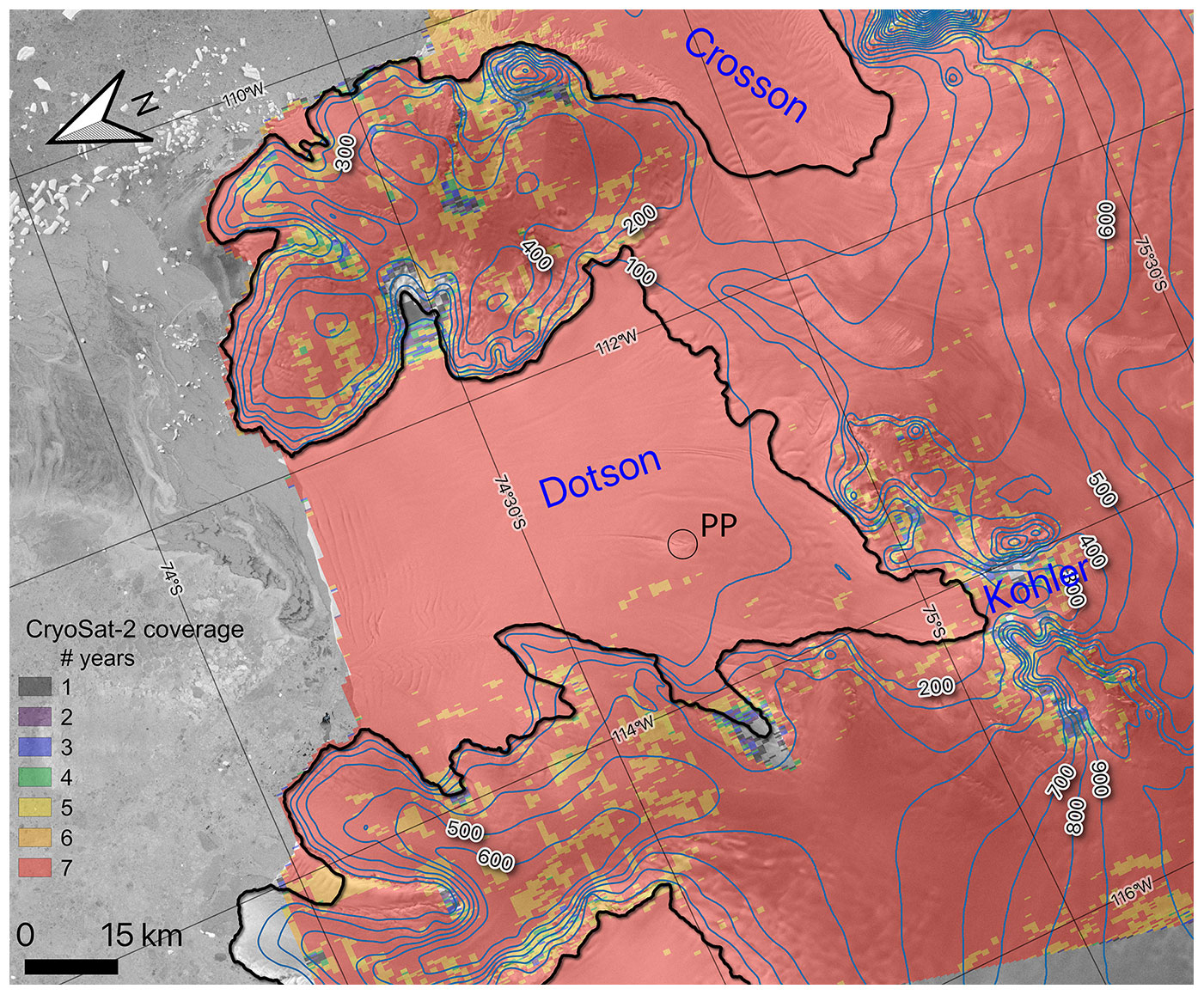
Figure 1 Overview of the test site with the Dotson and Crosson ice shelves marked along with the Kohler Glacier feeding the Dotson Ice Shelf. A pinning point on the ice shelf is marked with a circle and PP. The background image is the Radarsat Antarctic Mapping Project mosaic which has been overlaid with surface elevation contour lines (blue), the ASAID grounding line (black, Bentley et al., 2014), and the CryoSat-2 Swath coverage in the period from 2010–2016 with colors showing how many years are represented in each pixel (Matsuoka et al., 2021).

In this study we use the REMA strips in combination with CryoSat-2 measurements to obtain thinning and basal melt rates of the Dotson Ice Shelf at a 50 m spatial posting and a 3-yearly temporal resolution in the period from austral summer 2010/11 to 2017/18. We present and assess the high-resolution Basal melt rates Using REMA and Google Earth Engine (BURGEE) method. BURGEE is run on the Google Earth Engine (GEE), thereby allowing easy access to the data and fast processing on the GEE cloud computing platform (Gorelick et al., 2017). Furthermore, the use of GEE, REMA, and CryoSat-2 allows for easy upscalability. We use Dotson (Fig. 1) as a test site since there already exists a detailed basal melt rate study for comparison (Gourmelen et al., 2017). As mentioned, Gourmelen et al. (2017) relied fully on radar altimetry, which has limited coverage in mountainous regions. From Fig. 1 it is clear that this is an issue on parts of Dotson, which also becomes evident in the spatial coverage of the basal melt rates obtained in Gourmelen et al. (2017). For example the Kohler grounding zone (see Fig. 1) is poorly constrained, although here high melt rates are to be expected due to the intrusion of warm Circumpolar Deep Water into the ice shelf cavity (Jacobs et al., 1992). To investigate the highest feasible posting, we will perform a sensitivity study assuming that the highest uncertainties are related to the quality of the Lagrangian displacement. We will, furthermore, compare our results to the basal melt rates of Gourmelen et al. (2017) and discuss the different features we observe and the possible influence of a pinning point on basal channel formation and melt rates.

2 Theory

The basal mass balance and elevation change of an ice shelf can be observed in both a Eulerian and a Lagrangian framework. The Eulerian framework is fixed in space and provides information about the basal mass balance or elevation change at a given point in space. The Lagrangian framework, on the other hand, follows a given ice parcel and assesses the basal mass balance or elevation change of that parcel between two places in time, thereby taking the ice flow into consideration. In both cases the basal mass balance can be calculated through a mass conservation approach, which in a Lagrangian framework can be expressed as

$$\begin{array}{}\text{(1)}& {\displaystyle \frac{\text{D}H}{\text{D}t}}=-H(\mathrm{\nabla }\cdot \mathit{u})+{\dot{M}}_{\mathrm{s}}-{\dot{M}}_{\mathrm{b}},\end{array}$$

where $\frac{\text{D}H}{\text{D}t}$ is the Lagrangian ice thickness change; H is the ice thickness; ∇⋅u is the divergence of the ice flow; ${\dot{M}}_{\mathrm{s}}$ is the surface mass balance; and ${\dot{M}}_{\mathrm{b}}$ is the basal mass balance, defined as positive for melt. By assuming hydrostatic equilibrium, a constant ice density of ρ_i=917 kg m⁻³, and a constant seawater density of ρ_w=1025 kg m⁻³, the ice thickness can be approximated by

$$\begin{array}{}\text{(2)}& H=(h-h_{\mathrm{f}}){\displaystyle \frac{{\mathit{\rho }}_{\mathrm{w}}}{{\mathit{\rho }}_{\mathrm{w}}-{\mathit{\rho }}_{\mathrm{i}}}},\end{array}$$

where h is the ice shelf surface elevation and h_f the firn air content in meters of ice equivalent. Substituting Eq. (2) into Eq. (1) leads to

$$\begin{array}{}\text{(3)}& {\displaystyle \frac{\text{D}h}{\text{D}t}}-{\displaystyle \frac{\text{D}{h}_{\mathrm{f}}}{\text{D}t}}=(h-h_{\mathrm{f}})(\mathrm{\nabla }\cdot \mathit{u})+({\dot{M}}_{\mathrm{s}}-{\dot{M}}_{\mathrm{b}})\left({\displaystyle \frac{{\mathit{\rho }}_{\mathrm{w}}-{\mathit{\rho }}_{\mathrm{i}}}{{\mathit{\rho }}_{\mathrm{w}}}}\right),\end{array}$$

from which we can obtain the basal mass balance:

$$\begin{array}{}\text{(4)}& {\dot{M}}_{\mathrm{b}}={\dot{M}}_{\mathrm{s}}-\left({\displaystyle \frac{\text{D}h}{\text{D}t}}-{\displaystyle \frac{\text{D}{h}_{\mathrm{f}}}{\text{D}t}}+(h-h_{\mathrm{f}})(\mathrm{\nabla }\cdot \mathit{u})\right){\displaystyle \frac{{\mathit{\rho }}_{\mathrm{w}}}{{\mathit{\rho }}_{\mathrm{w}}-{\mathit{\rho }}_{\mathrm{i}}}}.\end{array}$$

3 Data

As can be seen from the basal mass balance Eq. (4), several auxiliary data sets are required to extract basal melt rates. In this section, we discuss the different data sets used in BURGEE to obtain and evaluate thinning and basal melt rates of the Dotson Ice Shelf.

3.1 Surface elevation

To obtain surface elevations of high temporal and spatial resolution we make use of the Reference Elevation Model of Antarctica (REMA, Howat et al., 2019). REMA consists of numerous digital surface model strips of either 2 or 8 m spatial resolution. They are based on stereo imagery from the WorldView and GeoEye satellites and acquired between 2010 and 2017. The strips are referenced to the WGS84 ellipsoid and are not co-registered. We have chosen to exclude all strips generated using the GeoEye satellites since they suffer from inconsistencies in the surface topography in the form of a striped pattern perpendicular to the satellite flight direction. Besides the strips, a REMA mosaic, made from multiple strips that have been co-registered with CryoSat-2 and ICESat (Howat et al., 2019), will be used as a reference surface to exclude outliers.

To correct the REMA strips for tilt and bias, elevation measurements from the radar altimeter aboard CryoSat-2 are used. CryoSat-2 was launched in 2010 and is the only ice-sheet-focused altimeter-carrying satellite which has been active throughout our entire study period ranging from austral summer 2010/11 to 2017/18. To transform the waveforms of the CryoSat-2 Level-1B SARin Baseline-D product to elevations with respect to the WGS84 ellipsoid, we use the leading-edge maximum gradient retracker presented in Nilsson et al. (2016). CryoSat-2 elevations are corrected for ocean loading tide, solid earth tide, geocentric polar tide, and dry and wet tropospheric and ionospheric effects using the data provided by ESA. Furthermore, the measurements are filtered using the ESA-provided quality flags. Additional ice-shelf-specific corrections are outlined in Sect. 4.1. The downside of using CryoSat-2 is that the radar signals may penetrate into the snowpack, thereby not measuring the direct surface but some depth into the snowpack. To study this effect, we compared CryoSat-2 measurements to those of the laser altimeter aboard ICESat-2 in the period from 2018 to 2021. From a comparison between neighboring measurements within 50 m and 5 d, we found a mean penetration depth of −0.4 m with a standard deviation of 2.1 m. We therefore assume that CryoSat-2 elevations can be considered to represent surface elevations.

Both the REMA strips and CryoSat-2 elevations are filtered for outliers by masking out elevations that differ more than 30 m from the REMA mosaic. This might filter out the advection of some large crevasses. However, since the REMA mosaic of Dotson is composed of REMA strips from mainly 2015 and 2016, this should mostly affect strips from the early years, if at all. After this filtering, both the REMA and CryoSat-2 elevation data are referenced to the Earth Gravitational Model 2008 geoid (Pavlis et al., 2012).

3.2 Surface velocity

Surface velocities are needed to calculate the ice flow divergence in the basal mass balance Eq. (4) and to perform a first-order displacement of the DEMs in the chain process of performing the Lagrangian displacement. The surface velocity data are obtained from the MEaSUREs ITS_LIVE data product (Gardner et al., 2022). These 120 m resolution surface velocities are generated using feature tracking of optical Landsat imagery. Since the velocity field of Dotson has shown no significant change throughout our study period (Lilien et al., 2018), we use the 120 m ITS_LIVE composite. Furthermore, we assume that the ice velocity does not vary with depth.

3.3 Surface mass balance

Since part of the observed ice shelf thickness change, or lack thereof, may be related to surface processes, monthly surface mass balance values (${\dot{M}}_{\mathrm{s}}$ in Eq. 4) are obtained from the regional climate model RACMO 2.3p3 (van Wessem et al., 2018). The output from RACMO is given in millimeters of water equivalent and translated into meters of ice equivalent by using an ice density of 917 kg m⁻³. We perform a spatial extrapolation since the 27 km grid does not cover the entire ice shelf. This is done by applying a linear extrapolation over a distance of 5 pixels. Finally, the data are interpolated onto the DEM grid from the original 27 km resolution grid using a bicubic interpolation.

3.4 Firn air content

To obtain the local ice equivalent thickness of the ice shelf, the presence of air in the firn layer needs to be taken into account (h_f in Eq. 2). Estimates of firn air content are obtained from the 27 km resolution IMAU-FDM v1.2A (Veldhuijsen et al., 2023) on a 10 d basis. The IMAU-FDM is forced with climate data from RACMO, which is why they share the same resolution. This also means that we apply an identical spatial extrapolation for the firn air content as for the surface mass balance (see Sect. 3.3) to ensure coverage over the entire ice shelf, followed by a bicubic interpolation onto the DEM grid.

3.5 Basal melt rate comparison products

To evaluate BURGEE we compare our results with two existing melt products, based on remote sensing and an ocean model, respectively. The remote-sensing-based product is obtained from CryoSat-2 swath measurements resulting in a mean basal melt rate product in the period from 2010–2016 at a 500 m resolution (Gourmelen et al., 2017, Fig. 6b). The ocean modeling product (LADDIE) is obtained by a 2D dynamical downscaling of the 3D ocean model MITgcm resulting in basal melt rates at a 500 m resolution (Lambert et al., 2023, Fig. 6c).

To investigate the basal melt pattern we further focus on the thermal forcing and the friction velocity provided by LADDIE, since basal melt can be approximated by the product of these two terms (e.g., Favier et al., 2019). The thermal forcing is the difference in temperature between the ocean water just below the ice shelf and the freezing point and can thereby be interpreted as the available heat to melt the ice. The friction velocity, defined as the time-mean ocean velocity just below the ice shelf, describes how effectively the heat is transported to the ice.

4 Methods

In the following sections we describe the methodology applied in BURGEE to calculate the basal melt rate using Eq. (4). Firstly, the REMA strips have to be transformed to digital elevation models by first accounting for dynamic and static corrections such as tides (see Sect. 4.1) and thereafter through a co-registration with CryoSat-2 (Sect. 4.2). A schematic overview of this procedure can be seen in Fig. 2. The resulting DEMs are then used to obtain both Eulerian (Sect. 4.3) and Lagrangian surface elevation changes (Sect. 4.5). The latter, along with ice flow divergences (Sect. 4.4), are used in the basal melt rate calculation (Sect. 4.5). Finally, a sensitivity study (Sect. 4.6) is performed to assess the highest feasible posting.

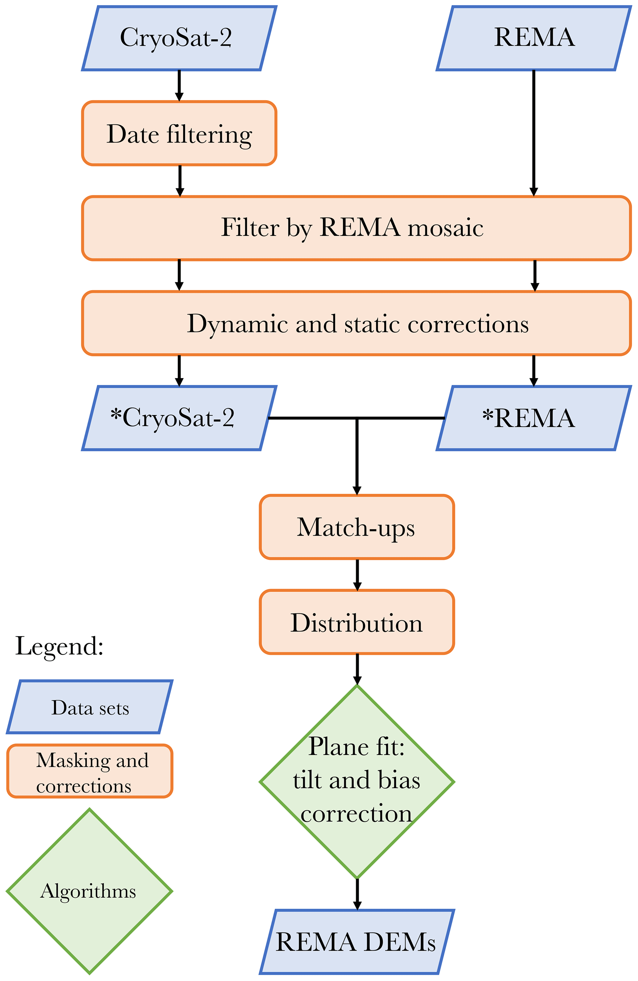
Figure 2 Flow chart showing the procedure going from WGS84-referenced CryoSat-2 and REMA digital surface model elevations to fully co-registered DEMs. The dynamic and static corrections are tides, mean dynamic topography, inverse barometer effect, and referencing to the geoid. The asterisk (*) denotes intermediate CryoSat-2 and REMA data sets, before merging the two and applying the two-fold co-registration as described in Sect.  4.2. One being with respect to the CryoSat-2 elevations and the other with respect to overlapping strips from the same period.

4.1 Dynamic and static corrections

Dynamic and static corrections have to be applied to both the REMA strips and the CryoSat-2 elevations to bring all elevations to the same reference frame regardless of variations in sea level.

Due to the underlying ocean beneath the ice shelf, tides (Δh_t), mean dynamic topography (Δh_mdt), and the inverse barometer effect (Δh_ibe) should also be taken into consideration in the ice shelf elevation corrections. Just like the geoid, the mean dynamic topography is a static correction, for which we use DTU15MDT, which is an updated version of DTU13MDT (Andersen et al., 2015). Tidal heights are obtained from the CATS2008 model on a 6 h interval at a ∼3 km spatial resolution for the REMA strips. Tidal heights for CryoSat-2, however, are obtained at their point locations and acquisition times. The inverse barometer effect was corrected for by using the 6 h NCEP/NCAR sea level pressure reanalysis data (Kalnay et al., 1996), from which residuals were calculated by using a mean sea level pressure of 1013 hPa. The residuals are then scaled by ∼0.9948 cm hPa⁻¹ to obtain the inverse barometer effect (Wunsch, 1972). The correction for the tide and inverse barometer effect are based on the acquisition time of the first stereo image. Since the ocean-induced corrections are only applicable to the ice shelf itself, the corrected surface elevation is obtained through

$$\begin{array}{}\text{(5)}& h=h_{\mathrm{data}}-\mathrm{\Delta }{h}_{\mathrm{geoid}}-\mathit{\alpha }\left(\mathrm{\Delta }{h}_{\mathrm{t}}+\mathrm{\Delta }{h}_{\mathrm{mdt}}+\mathrm{\Delta }{h}_{\mathrm{ibe}}\right),\end{array}$$

where h_data is either the CryoSat-2 or REMA surface elevations, Δh_geoid is the offset to the geoid, and α is a coefficient ensuring a smooth transition from grounded to floating ice as in Shean et al. (2019). This transition is a function of the distance to the grounding line (l), based on the ASAID product of Bentley et al. (2014):

$$\begin{array}{}\text{(6)}& \mathit{\alpha }\left(l\right)=\left\{\begin{array}{ll}\mathrm{0}& l\le \mathrm{0}\mathrm{km}\\ \frac{\mathrm{1}}{\mathrm{3}}l& \mathrm{0}\mathrm{km}<l\le \mathrm{3}\mathrm{km}\\ \mathrm{1}& l>\mathrm{3}\mathrm{km}\end{array}\right..\end{array}$$

Once the corrections have been applied the elevation data are at the stage marked with an asterisk (*) in Fig. 2.

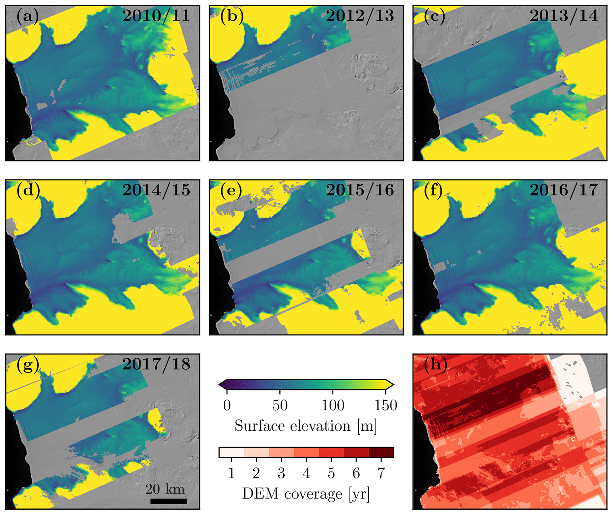
Figure 3 Yearly co-registered DEM mosaics ranging from 2010/11 (a) to 2017/18 (g). Notice that there are no data from 2011/12. (h) Heat map showing the total DEM coverage.

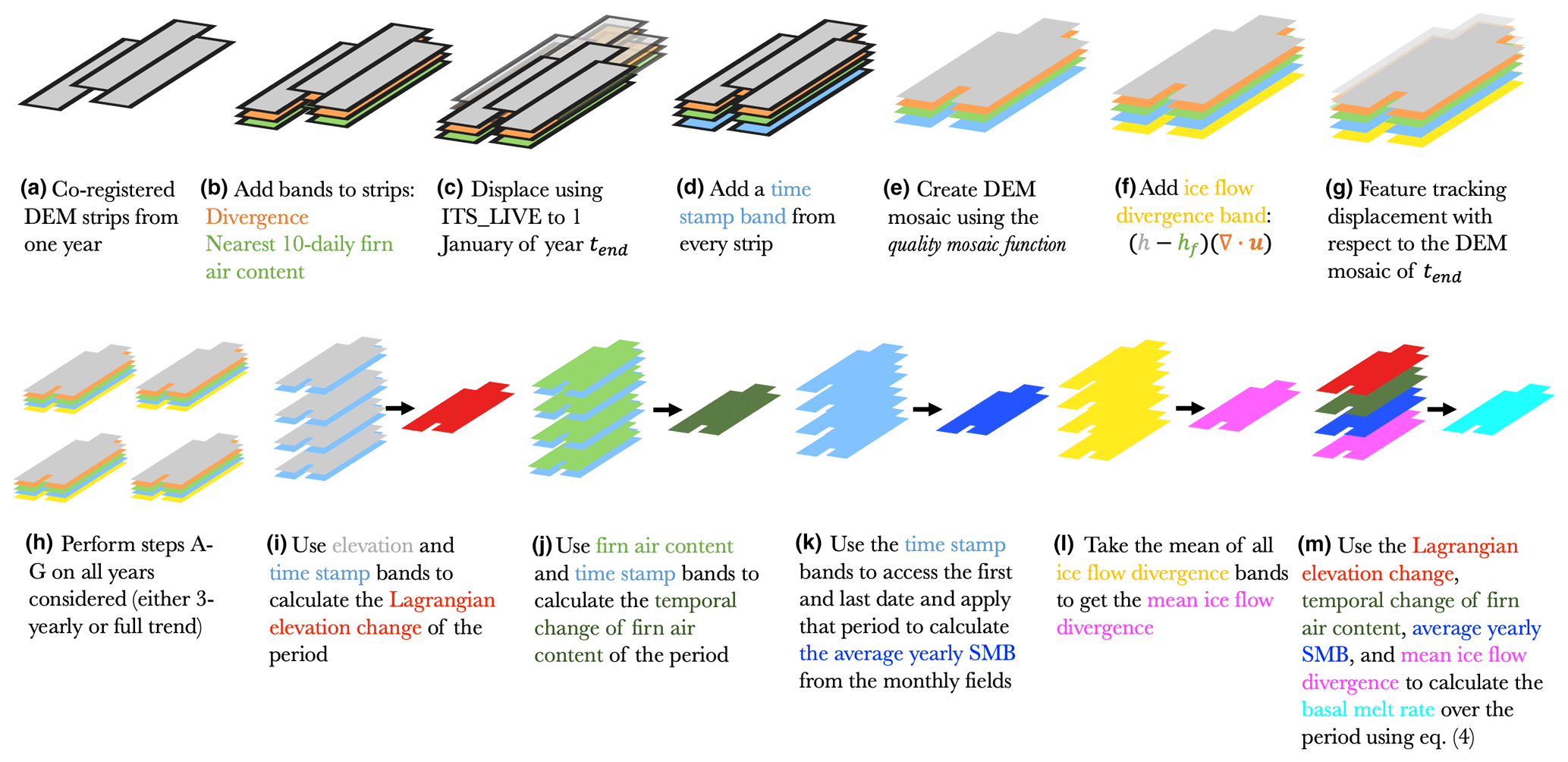
Figure 4 The workflow used to go from co-registered DEM strips in panel (a) to Lagrangian displaced DEM mosaics in panel (g), with all Lagrangian displaced mosaics in panel (h) used to assess the Lagrangian elevation change in panel (i) and the basal melt rate in panel (m).

4.2 Co-registration

Since the REMA strips have not been co-registered with the actual surface elevation, strips might be both tilted and vertically misplaced. A co-registration with actual surface elevations therefore is needed. Here, the co-registration of the REMA strips is performed by using two consecutive plane-fit co-registration approaches: first with respect to the CryoSat-2 measurements and second with respect to overlapping REMA strips. The double co-registration is performed to improve the quality, as there might still be small offsets between strips where they overlap. The co-registration with CryoSat-2 is done by correcting for tilt and vertical bias after fitting a plane through the residuals between CryoSat-2 and the individual REMA strips.

Before the co-registration of a REMA strip with CryoSat-2 can be performed, we defined four criteria that should be fulfilled in the given order: (i) the CryoSat-2 elevations used to perform the co-registration have to be within 1 month of the acquisition date of the REMA strip to ensure that the CryoSat-2 elevations are representative of the elevations when the strip was acquired; (ii) for each and every REMA strip the number of available CryoSat-2 measurements/matchups that have fulfilled criterion (i) should be at least 80 to ensure that we perform a representative plane fit. This threshold has been set through trial and error and is a balance between good-quality co-registration while keeping a sufficient number of REMA strips; (iii) the northernmost and southernmost CryoSat-2 points should be at least 60 km apart. Likewise, the CryoSat-2 points furthest separated in the longitudinal direction should be at least 10 km apart. This third criterion ensures that the CryoSat-2 measurements are evenly distributed over the REMA strip. This is a rather conservative threshold, which may filter out smaller but good-quality REMA strips. However, in this way we ensure the best possible DEM quality, which is crucial to resolve small-scale features.

The second co-registration is performed on a yearly basis by co-registering all DEMs that overlap at least 25 % with the yearly median DEM. The yearly median DEM is the median of all overlapping REMA DEM strips per year, with 1 July defined as the first day of the year. The residuals between the DEM strips and the median DEM are thus used to perform the plane fit. The second co-registration is thereby not applied to all strips.

The co-registered DEM strips range from austral summer 2010/11 to 2017/18 and have a yearly coverage of up to 98 % in 2016/17 (see Fig. 3).

4.3 Eulerian elevation change

Besides the Lagrangian elevation change which is needed to calculate the basal mass balance, we also assess the elevation change in a Eulerian framework. This provides information about where the ice shelf is thinning and thickening.

The Eulerian elevation change is calculated as a linear trend on a tri-yearly basis and throughout the entire study period. A tri-yearly period is chosen as the highest temporal resolution due to the limited to no DEM coverage in 2011/12 and 2012/13 (Fig. 3), along with the limited coverage of the center part of the ice shelf in 2015/16 and 2017/18 (Fig. 3). In this study, 1 July is defined as the start of the year, putting the austral summer in the middle of a year, with the first year of our study period being 2010/11 and the last year 2017/18. The Eulerian elevation change is thus calculated from the co-registered DEMs by applying a linear fit to the DEM strips and their corresponding time stamp, where the latter may vary from pixel to pixel. This implies that both the tri-yearly and entire study period trends are produced from all strips available in the period considered. The Eulerian elevation change is further cleaned from possible outliers by removing points with a surface elevation change rate of more than ±15 m yr⁻¹.

4.4 Divergence of the velocity field

Berger et al. (2017) illustrated the impact different methods of calculating the velocity gradients have on the resulting divergence. They found regularized divergences (Chartrand, 2011) to be the best choice, since this method suppresses noise while keeping the data signal (Chartrand, 2011; Berger et al., 2017). In this study we use total-variation regularization (Chartrand, 2017), which is an updated version of the regularization method presented in Chartrand (2011) made especially for multidimensional data, to compute the gradients of the 120 m resolution ITS_LIVE velocity field. Due to our previous assumption of a constant velocity field in time, we also assume that the resulting divergence field of Dotson is constant in time. Finally, the divergence field is linearly interpolated onto the DEM grid.

4.5 Lagrangian elevation change and basal melt rate

As for the Eulerian elevation change, both the Lagrangian elevation change and the basal mass balance are calculated on a tri-yearly basis and as a linear trend throughout the entire study period. The whole process of obtaining the Lagrangian elevation change from the co-registered DEM strips and further steps to assess the basal mass balance is shown in Fig. 4 and is further outlined in this section.

The Lagrangian displacement is performed on a yearly basis using 1 July as the start of the year, putting the austral summer in the middle of a year. Together with the DEM strips, we also displace the velocity divergence and the nearest 10-daily firn air content from IMAU-FDM (Fig. 4b).

The most common approach to perform the Lagrangian displacement of DEMs is using a velocity field (i.e., Moholdt et al., 2014) or applying a feature tracking algorithm (i.e., Berger et al., 2017). The first approach requires velocities of high quality and resolution and puts strong restrictions on the spatial resolution of the final product. It is, however, computationally efficient, whereas the latter approach is computationally heavy but allows for a higher output spatial resolution. In BURGEE we want to keep the spatial resolution high, while keeping the computational cost low to allow for future study region upscaling. To do so, we first apply a velocity displacement, after which we perform a final correction through feature tracking. This decreases the search window needed in the feature tracking process, thus reducing the computational time.

The initial displacement of the DEM strips is performed by using the ITS_LIVE surface velocities, where all DEMs from the year considered are displaced to 1 January of the final year (t_end) in the trend period (Fig. 4c). For the Lagrangian elevation change of the entire period, t_end is thus 1 January 2018, and for the tri-yearly 2010/11–2013/14, t_end will be 1 January 2014. This means that all DEMs are roughly aligned to where they would be located at t_end. However, surface features such as crevasses may not be perfectly aligned, for which the second displacement is needed.

Before the second displacement is performed, all DEM strips are accompanied with a time stamp band (Fig. 4d), and a DEM mosaic of the given year is created using the quality mosaic function in GEE (Fig. 4e). This is done to reduce the computational requirements of the feature tracking algorithm. The resulting elevation, firn air content, and velocity divergence mosaics are used to add an ice flow divergence band (Fig. 4f) according to the ice flow divergence term ($(h-h_{\mathrm{f}})(\mathrm{\nabla }\cdot \mathit{u})$) in Eq. (4).

This second and final displacement is performed by using the built-in feature tracking algorithm displacement in GEE, which uses orientation correlation. In this displacement, the DEM mosaic of the given year is referenced to that of t_end, thereby aligning all surface features to their position in the DEM mosaic from t_end (Fig. 4g). The built-in feature tracking algorithm on the GEE takes in three adjustable parameters: patch width, max offset, and stiffness, which were set to 100 m, 300 and 3, respectively. The patch width defines the size of the patches/regions to search for within the distance given by max offset, whereas the stiffness parameter defines how much distortion/warping is allowed. Since ice features may very well change in shape, a lower less rigid stiffness parameter is desired.

The above-mentioned steps (Fig. 4a–g) are then performed on all years considered, and the Lagrangian elevation change using the displaced DEM mosaics is then obtained similarly to the Eulerian elevation change by applying a linear fit to the DEM mosaics and their corresponding time stamp (Fig. 4i), which in this case may vary from pixel to pixel. The same outlier criterion of 15 m yr⁻¹ is used to mask out the remaining possible outliers. This filter could possibly filter out fast, small-scale processes like rift opening, which is acceptable for this study, given our focus on the basal melt rates.

To calculate the final basal melt rate using Eq. (4), the change of firn air content with time is calculated using the time and firn air content bands (Fig. 4j). Furthermore, the time stamp bands are used to access the first and last date of the given period (full study period or 3-yearly period) and use those as limits to calculate the average yearly surface mass balance from the monthly RACMO fields within the period limits (Fig. 4k). Also, a mean of all ice flow divergence bands is taken to get the mean ice flow divergence of the period (Fig. 4l). Joining all of this with the Lagrangian elevation change and the constant densities for ice and seawater allows for the basal melt rate to be calculated over the desired period (Fig. 4m). As for the Eulerian elevation change (Sect. 4.3), this implies that both the tri-yearly and entire study period trends are produced from all strips available in the period considered and that some pixels may not have data from all years considered.

4.6 Sensitivity experiment

Since the signal-to-noise ratio of basal mass balance is expected to increase when refining the spatial posting, we performed a synthetic experiment to assess the impact of spatial posting on the basal melt rate in BURGEE. The sensitivity experiment is based on the assumption that the Lagrangian displacement is one of the main contributors to the basal melt rate uncertainty. Within this experiment we used the aligned annual DEM mosaics from 2010/11 and 2014/15, since they have a high coverage and are relatively far apart in time, thus placing stronger requirements on the displacement algorithm applied. Based on both aligned annual DEM mosaics, two different basal mass balance maps are obtained using two different Lagrangian elevation changes. This is first done from the aligned DEM mosaics resulting in the true basal melt rate. Second, the otherwise aligned 2010/11 DEM mosaic is displaced based on the 4-year accumulated ITS_LIVE error fields to create an alternative aligned DEM mosaic that incorporates the displacement uncertainty due to velocity errors. The Lagrangian elevation change is then calculated using the error-displaced 2010/11 DEM mosaic and the previously mentioned 2014/15 DEM mosaic. The difference between the resulting basal melt rates following from the two Lagrangian elevation changes is then calculated at a 50, 100, 250, and 500 m posting to see what posting is required for the artificial error to cancel out. The 500 m posting corresponds to what has been used when using CryoSat-2 alone (Gourmelen et al., 2017) and therefore serves as our most coarse limit.

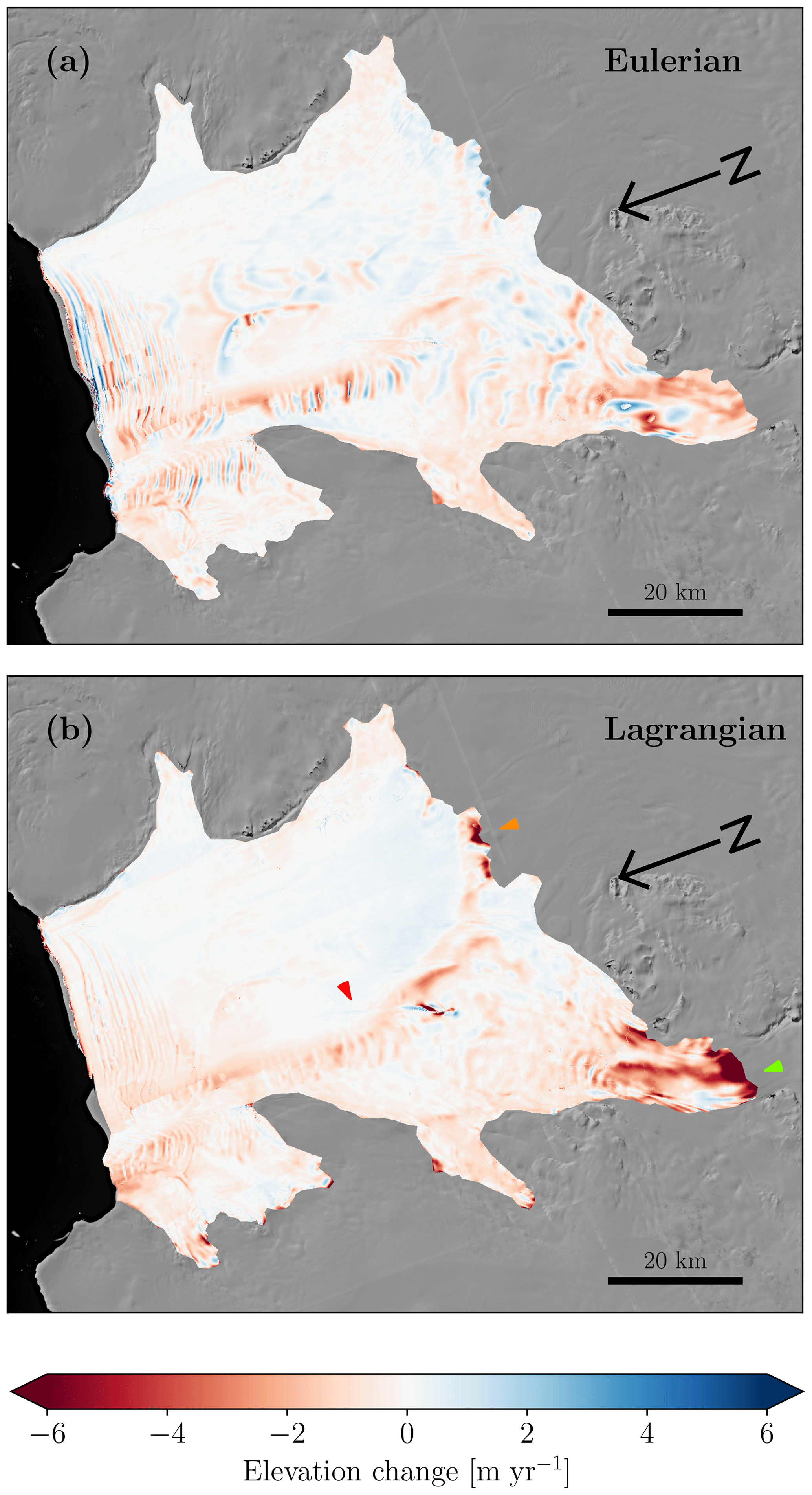
Figure 5 Eulerian (a) and Lagrangian (b) surface elevation trends from 2010/11–2017/18 at a 50 m posting. The red arrow marks the main channel, the green arrow marks the Kohler grounding zone, and the orange arrow marks the high elevation changes towards the Crosson Ice Shelf.

5 Results

5.1 Evaluation of BURGEE results

The Eulerian and Lagrangian surface elevation trends over the entire study period (2010/11–2017/18) are shown in Fig. 5 at a 50 m posting. Owing to its along-flow coordinate system, the Lagrangian elevation change has a much smoother pattern compared to the Eulerian framework. In both frameworks, the channel described by Gourmelen et al. (2017) (red arrow), which we will refer to as the Dotson Melt Channel hereafter, shows pronounced thinning. The Eulerian elevation change shows elevation decrease along and west of the Dotson Melt Channel, whereas the area east of this channel shows a more irregular pattern. Similarly, we see almost no elevation change in this eastern zone in the Lagrangian elevation change and a smoother pattern due to the along-flow framework. Three areas stand out with high Lagrangian elevation changes, namely the Dotson Melt Channel (red arrow), at the border towards the Crosson Ice Shelf (orange arrow), and the grounding zone at the inflow of the Kohler Glacier (green arrow). The latter is not fully resolved in Gourmelen et al. (2017), presumably due to limited CryoSat-2 coverage (Fig. 1).

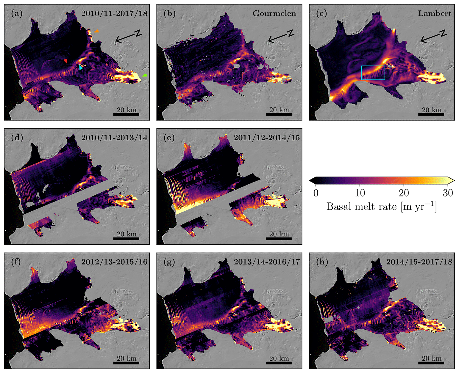
Figure 6 (a) Basal melt rate trend from 2010/11 to 2017/18. The arrows point out the Dotson Melt Channel (red), the pinning point below the ice shelf (cyan), the Kohler grounding zone (green), and the high melt rates near the Crosson Ice Shelf. (b) Basal melt rate from Gourmelen et al. (2017). (c) Basal melt rate from Lambert et al. (2023) with the box marking the zoom-in in Fig. 9. (d–h) Tri-yearly basal melt rate trends.

The basal melt rate at a 50 m posting over the entire study period can be seen in Fig. 6a, which shows a similar pattern to the Lagrangian elevation change. Figure 6d–h show the 3-yearly basal melt rate trends also at a 50 m posting. There is a clear spatial consistency throughout the entire period, though melt rate magnitudes do seem to show temporal variability. A striped pattern is visible on some of the 3-yearly maps (e.g., 2011/12–2014/15, Fig. 6e, and 2012/13–2015/16, Fig. 6f) due to the DEM mosaic coverage seen in Fig. 3. The varying coverage also implies that the trend is taken over different time periods whenever there is missing data in the DEM mosaics and that gaps may occur if less than 2 years of data are available. Furthermore, the Lagrangian displacement is performed with respect to the latest DEM mosaic (Sect. 4.5), which is what is causing the higher melt rates in the center of Dotson in the 2012/13–2015/16 product. Focusing on the basal melt rate of the entire study period (Fig. 6a) we see that high melt rates are present along the Dotson Melt Channel (red arrow), with a melt convergence zone just east of a pinning point (cyan arrow), near the Kohler grounding zone (green arrow), and towards the Crosson Ice Shelf (orange arrow). These are all features that are present in both Gourmelen et al. (2017) (Fig. 6b) and Lambert et al. (2023) (Fig. 6c). Likewise, the overall pattern is similar in all three products. A slight exception to this is the melt signal near the calving front seen in BURGEE. Here, there are large crevasses and fractures in the ice shelf, which may not be well represented in the divergence signal when assessing the basal melt rate at a 50 m posting. Overall, BURGEE allows us to derive melt rates of all parts of the ice shelf, compared to the limited coverage especially near the ice shelf margin for Gourmelen et al. (2017).

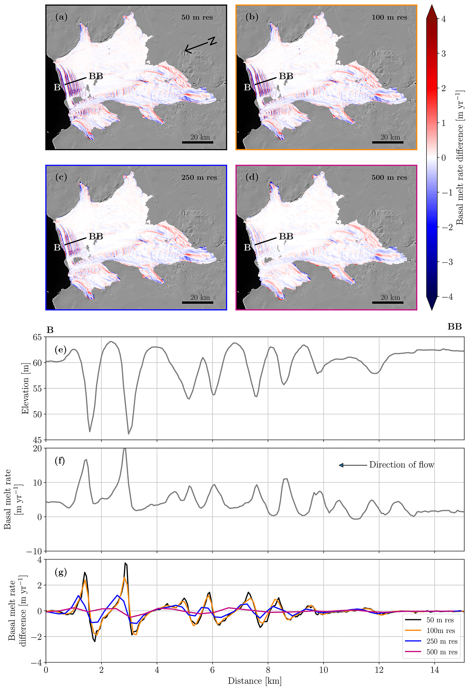
Figure 7 (a–d) The difference between the basal melt rate obtained from the correct and the erroneous Lagrangian elevation changes at 50 m (a), 100 m (b), 250 m (c), and 500 m (d) postings. (e) The perfectly aligned 2010/11 DEM mosaic at the B–BB cross section. (f) The basal melt rate obtained from the correct DEMs at the B–BB cross section. (g) The basal melt rate differences at the B–BB cross section at 50, 100, 250, and 500 m postings. Note that panels (f) and (g) use a different range on the y axis.

5.2 Results from the sensitivity experiment

Figure 7 shows the result of the sensitivity study where we created an alternative aligned DEM mosaic by displacing the correctly aligned DEM based on the error of the ITS_LIVE velocities under the assumption that the quality of the Lagrangian displacement is the main contributor to the basal mass balance uncertainties. In the part of the ice shelf with fewer surface undulations (distances 10–15 km of the B–BB cross section), the basal melt rate differences resulting from the artificial displacement cancel out to a large degree already at a 50 m posting. In areas with stronger surface undulations, it requires a coarser posting for the differences to cancel out. However, it should be noted that even at a high posting of 50 m, the resulting differences in basal melt rates of the cross section are within ±4 m yr⁻¹. Furthermore, the largest differences correlate with high melt rates. Based on these findings, we have chosen to offer our product at a 50 and a 250 m posting (https://doi.org/10.4121/21841284, Zinck et al., 2023). It should be noted, however, that the Lagrangian displacement is not the only error source, since all data and assumptions used to calculate the basal mass balance (Eq. 4) come with errors and uncertainties, which is why these numbers cannot be considered as true uncertainties of the final product.

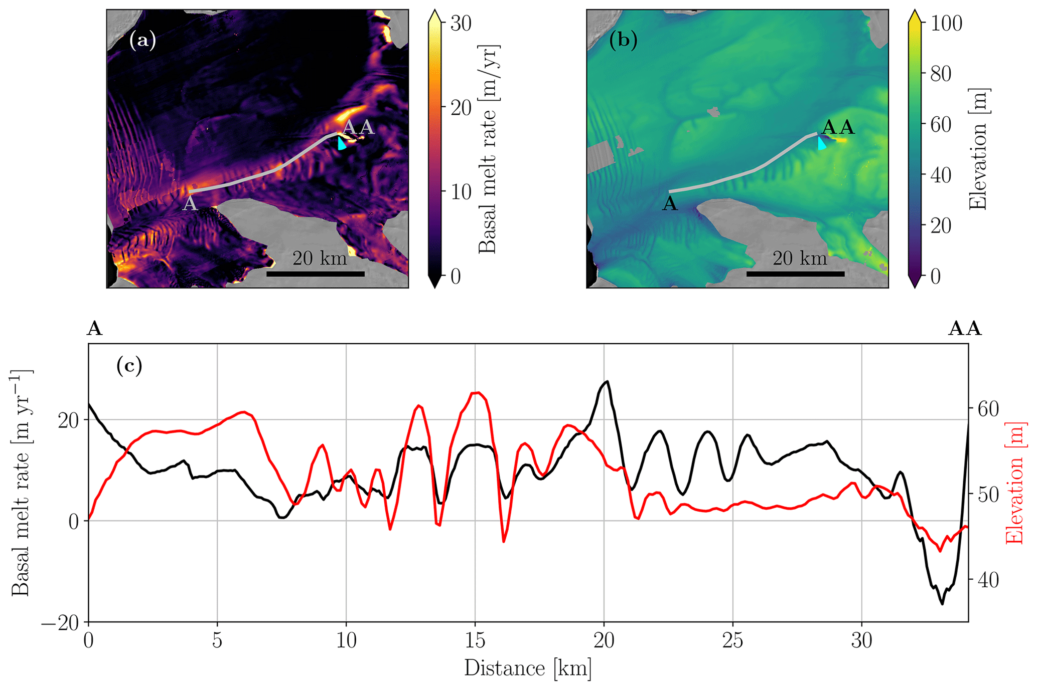
Figure 8 (a) Basal melt rate from 2010/11–2017/18; (b) 2016/17 DEM, with the gray line marking the cross section A to AA in panel (c); (c) surface elevation from the 2016/17 DEM (red line), prior to any Lagrangian displacement, and basal melt rate (black line) at the cross section marked in panel (a) and (b). The distance in panel (c) is with respect to the left end point (A) of the gray line in panel (a) and (b).

5.3 Interpretation of the melt pattern

In the vicinity of the pinning point (Fig 6a, cyan arrow), the basal melt within the Dotson Melt Channel shows a smooth pattern which changes to a more wavey pattern downstream. Roberts et al. (2018) hypothesize that such a wavey pattern can originate near pinning points due to ocean heat variability, where periods of increased available ocean heat induce enhanced thinning and a reduced back stress over the pinning point and vice versa. Through convergence and divergence, the resultant temporal variability in ice speed translates into an alternating pattern of thick and thin ice. To investigate the influence of the pinning point on the spatial melt variability within the Dotson Melt Channel, we have focused on a transect following the basal channel from the pinning point to the ice shelf front (Fig. 8, transect A to AA and pinning point marked with the cyan arrow). We can see clear surface undulations along the Dotson Melt Channel that emerge downstream from the pinning point. We also notice higher melt rates coinciding with these surface undulations, especially around 12–22 km, where we see that higher melt rates align with higher surface elevations, implying deeper basal drafts, and vice versa.

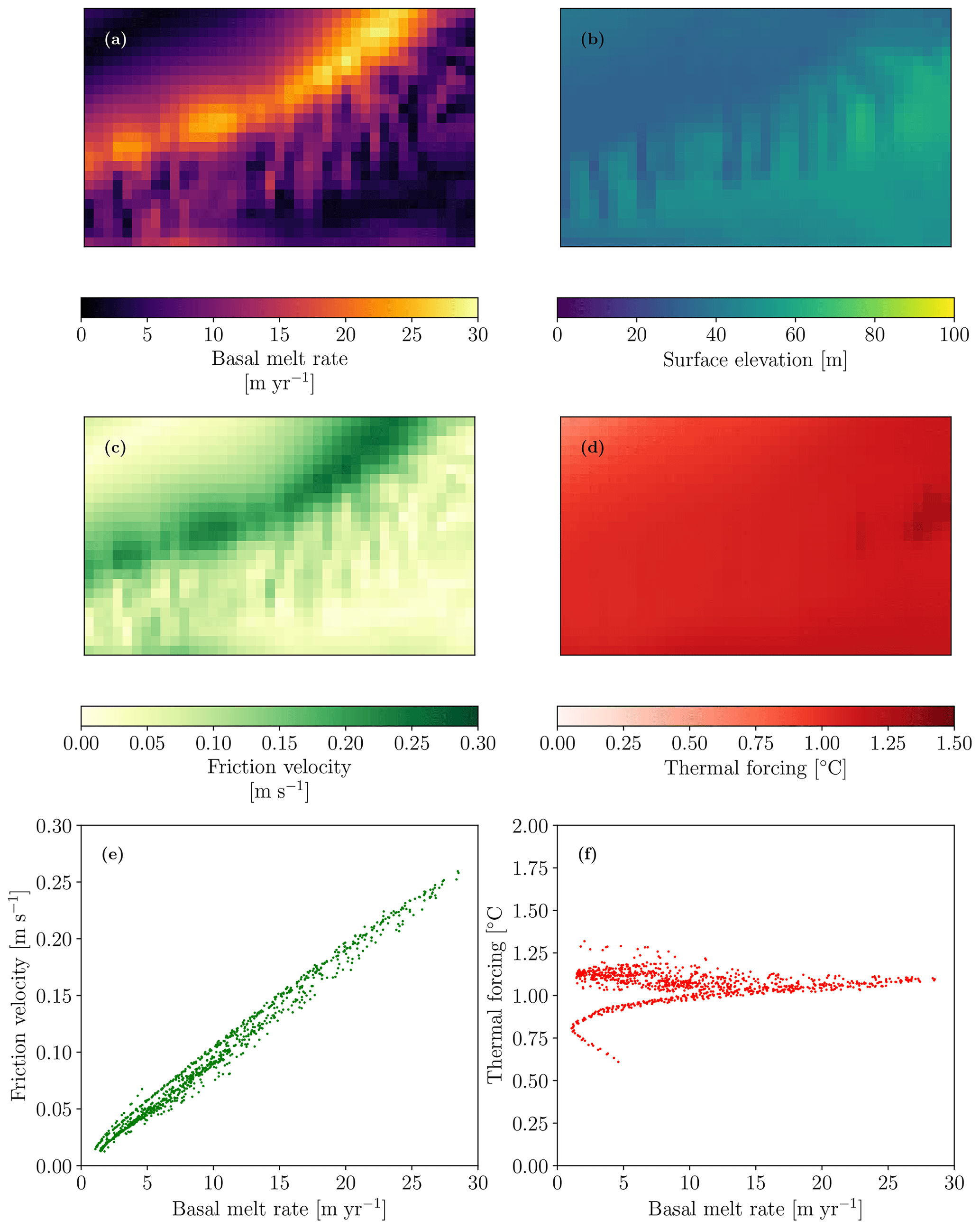
Figure 9 Model outputs from LADDIE within the box marked in Fig. 6c: (a) basal melt, (b) surface elevation, (c) friction velocity, (d) thermal forcing, (e) friction velocity as a function of basal melt, and (f) thermal forcing as a function of basal melt.

To investigate the relation between the surface undulations and the basal melt rate, we disentangle basal melt into its two major components: thermal forcing and friction velocity. The thermal forcing determines the locally available heat for melting, whilst the friction velocity determines the efficiency of turbulent heat exchange toward the ice shelf base. The thermal forcing and friction velocity, simulated by LADDIE, are shown in Fig. 9, along with the LADDIE basal melt rates and draft. A direct comparison between the LADDIE thermal forcing and friction velocity with the BURGEE melt rates cannot be done, since LADDIE is forced with a different ice shelf geometry; therefore, we compare to the LADDIE melt rates instead. Figure 9e–f further shows the friction velocity and the thermal forcing as a function of the melt rate, respectively. It is evident that the friction velocity has a high correlation with the melt rate, implying that it is the main driver of spatial melt variability at fine scales. The friction velocity is affected by the undulations. Where the meltwater plume encounters thick ice, it is squeezed vertically, leading to convergence and a local acceleration. This locally enhanced friction velocity increases the heat transfer and consequently the basal melt. As basal melt is typically highest in regions of thick ice (Fig. 8), this interaction between ice topography and melt is a negative feedback that should smoothen out the undulations downstream. This negative feedback may explain the weakening signature of the undulations towards the ice shelf front.

6 Discussion

We show how REMA in combination with CryoSat-2 is capable of obtaining high-resolution basal melt rates of the Dotson Ice Shelf. The use of CryoSat-2 and Google Earth Engine in BURGEE allows us to process significantly more REMA strips than if using Operation IceBridge alone, and it allows for fast computations. We observe the same large-scale melt pattern consisting of one wide melt channel (Dotson Melt Channel) as previous studies (Gourmelen et al., 2017; Lambert et al., 2023). Additionally, BURGEE allows us to observe small-scale melt features which would go unnoticed in lower-resolution altimetry-based products such as Gourmelen et al. (2017) and Adusumilli et al. (2020). This especially becomes evident within the Dotson Melt Channel.

Our elevation maps reveal that surface undulations appear downstream of a pinning point on the ice shelf. Here, we also find a correlation between melt rates and ice thickness along the Dotson Melt Channel. The link between surface undulations and basal melt rates is further supported by Watkins et al. (2021), who found a clear relationship between pinning points and roughness and a correlation between the latter and basal melt. Furthermore, modeling studies suggest shear zones and topographic features have a possible impact on basal channels and their formation (Gladish et al., 2012; Sergienko, 2013). Also, Roberts et al. (2018) suggest that varying ocean temperatures lead to ice shelf thickness change and thereby a change in the back stress over ice rumples causing a wavey pattern as the one we observe being initialized at the pinning point. Model output from LADDIE suggests that the friction velocity is the driver of the increased melting in regions of greater ice thickness, due to compression and divergence of the melt plume. The large-scale pattern of the Dotson Melt Channel, bending towards the western margin of the ice shelf, is explained by buoyancy forcing of the low-salinity meltwater plume (Lazeroms et al., 2018). However, just eastward of the pinning point, a convergence zone, causing a narrow sharp plume with high melt rates, indicates that the Dotson Melt Channel pathway may also be influenced by the pinning point. Meltwater plumes causing channel formation have a tendency to occur at western topographic boundaries in this area of Antarctica (Lambert et al., 2023). The eastward melt convergence zone suggests that the pinning point is big enough to act as a western topographic feature. Without the pinning point the meltwater plumes may thus converge elsewhere. We therefore postulate that the pinning point impacts the spatial variability within the Dotson Melt Channel and possibly also the channel pathway due to the convergence zone just east of the pinning point.

Varying basal melt rates can also be seen within the Dotson Melt Channel in Gourmelen et al. (2017), but due to the coarser resolution and gaps in the data, it is not clear whether this variation is (partially) due to noise or actual signal. This underlines the importance of high-resolution basal melt rates.

Finally, the spatial coverage is improved when using a combination of REMA and CryoSat-2. CryoSat-2 on its own cannot cover all parts of an ice shelf, especially those surrounded by topographic features such as mountains. Furthermore, we can assess temporal changes on a 3-yearly basis but with poorer coverage than the full trend due to the yearly REMA coverage. Using elevation data from the CryoSat-2 swath mode alone (Gourmelen et al., 2017) would likely yield a higher temporal resolution but would not resolve the small-scale features which we can capture with BURGEE. Adusumilli et al. (2020) used a wide range of remotely sensed surface elevations to obtain basal melt rates at quarter-yearly resolution but at the cost of the spatial resolution. The Dotson Ice Shelf did not show noticeable changes in basal melt over the study period; however, ocean observations from the Dotson Ice Shelf cavity do show variations on seasonal timescales of inflow of warm Circumpolar Deep Water (Jenkins et al., 2018; Yang et al., 2022). This could imply seasonal variability in the basal melt rates, as has been observed at both the Nivlisen Ice Shelf in East Antarctica (Lindbäck et al., 2019) and the Filchner–Ronne Ice Shelf (Vaňková and Nicholls, 2022). To investigate seasonal changes using BURGEE, more DEMs than currently available from REMA would be needed. If REMA-2 or similar data products based on future missions were to provide such a higher temporal coverage, studying seasonal or interannual variations in basal melt would become within reach with BURGEE.

The clear advantage of BURGEE is the high spatial resolution and the use of Google Earth Engine. The latter allows one to efficiently and rapidly process large amounts of data, while the built-in data catalogue drastically reduces the amount of data which has to be downloaded locally. Furthermore, the choice for no site-specific tuning allows the methodology to be easily applied to other ice shelves in Antarctica. By incorporating upcoming and more up-to-date elevation data sets, we might then be able to assess basal melting at 50 m posting and at greater temporal resolution than 3 years. By doing so to other ice shelves influenced by pinning points, our product may also help answer what the effect of those are on the basal melt pattern. But, more importantly, it would help us to assess the (in)stability of other ice shelves and locate weak spots on them.

7 Conclusions

In this study we have shown that the Reference Elevation Model of Antarctica can be used to obtain high-resolution surface elevation changes and basal melt rates of the Dotson Ice Shelf. We perform a sensitivity study which supports the trustworthiness of the observed small-scale features. It further indicates that a 50 m spatial posting of basal melt is feasible. BURGEE reveals spatial variability within the Dotson Melt Channel, which was not fully resolved in coarser remote sensing products. We find strong indications that a pinning point on the ice shelf influences this spatial melt variability within the Dotson Melt Channel and that it may be controlling the position of a warmer ocean plume, thereby impacting the pathway of the Dotson Melt Channel. This underlines the importance of high-resolution basal mass balance products as our product can help future studies to provide answers to the causes behind them.

Finally, BURGEE contains no site-specific tuning, which means that it can easily be applied to other ice shelves. Of course, our assumption of a constant velocity field in time does not hold for all ice shelves and should thus be adjusted. Nonetheless, with the right computing sources, this study could be upscaled to a pan-Antarctic study of high-resolution basal mass balances.