The stability of present-day Antarctic grounding lines – Part 2: Onset of irreversible retreat of Amundsen Sea glaciers under current climate on centennial timescales cannot be excluded

Observations of ocean-driven grounding-line retreat in the Amundsen Sea Embayment in Antarctica raise the question of an imminent collapse of the West Antarctic Ice Sheet. Here we analyse the committed evolution of Antarctic grounding lines under the present-day climate. To this aim, we first calibrate a sub-shelf melt parameterization, which is derived from an ocean box model, with observed and modelled melt sensitivities to ocean temperature changes, making it suitable for present-day simulations and future sea level projections. Using the new calibration, we run an ensemble of historical simulations from 1850 to 2015 with a state-of-the-art ice sheet model to create model instances of possible present-day ice sheet configurations. Then, we extend the simulations for another 10 000 years to investigate their evolution under constant present-day climate forcing and bathymetry. We test for reversibility of grounding-line movement in the case that large-scale retreat occurs. In the Amundsen Sea Embayment we find irreversible retreat of the Thwaites Glacier for all our parameter combinations and irreversible retreat of the Pine Island Glacier for some admissible parameter combinations. Importantly, an irreversible collapse in the Amundsen Sea Embayment sector is initiated at the earliest between 300 and 500 years in our simulations and is not inevitable yet – as also shown in our companion paper (Part 1, Hill et al., 2023). In other words, the region has not tipped yet. With the assumption of constant present-day climate, the collapse evolves on millennial timescales, with a maximum rate of 0.9 mm a⁻¹ sea-level-equivalent ice volume loss. The contribution to sea level by 2300 is limited to 8 cm with a maximum rate of 0.4 mm a⁻¹ sea-level-equivalent ice volume loss. Furthermore, when allowing ice shelves to regrow to their present geometry, we find that large-scale grounding-line retreat into marine basins upstream of the Filchner–Ronne Ice Shelf and the western Siple Coast is reversible. Other grounding lines remain close to their current positions in all configurations under present-day climate.

1 Introduction

The potential for the West Antarctic Ice Sheet (WAIS) to collapse in response to global warming was first raised as a concern by Mercer (1978). This collapse would be driven by the marine ice sheet instability (MISI; Weertman, 1974; Schoof, 2007, 2012) and would raise global sea levels by about 3 m in the long term (Feldmann and Levermann, 2015a). Over the past decades, the Antarctic Ice Sheet has been losing mass (Smith et al., 2020) at an increasing rate (The IMBIE team, 2018; Rignot et al., 2019), with current mass losses being driven by buttressing loss of ice shelves through increased ocean-driven melting (Gudmundsson et al., 2019). In particular, retreat of grounding lines – the boundary separating the grounded parts of the ice sheet from its floating ice shelves – and increased mass loss in the Amundsen Sea Embayment (ASE) sector (Rignot et al., 2019; Milillo et al., 2022) have raised the question of whether a collapse of the West Antarctic Ice Sheet driven by MISI might already be underway (Rignot et al., 2014; Mouginot et al., 2014; Joughin et al., 2014; Favier et al., 2014). Several numerical modelling studies find continued retreat in the ASE under current climate conditions (Joughin et al., 2014; Favier et al., 2014; Seroussi et al., 2017; Arthern and Williams, 2017). Also, the commitment to large-scale retreat was found to be possible close to present-day climate conditions: Garbe et al. (2020) report that retreat of West Antarctic grounding lines could occur at around 1–2 ^∘C of global warming above pre-industrial levels, which would correspond to a regional warming of 1.8–3.6 ^∘C in the atmosphere and 0.7–1.4 ^∘C in the ocean surrounding the Antarctic Ice Sheet. Golledge et al. (2021) find that, in a simulation of the last interglacial, the West Antarctic Ice Sheet starts retreating after 1500 years with constant current climate conditions. These findings raise the importance of a systematic analysis to identify whether Antarctic grounding lines are currently engaged in an irreversible retreat due to MISI, and to gain a more detailed understanding of the committed retreat under present-day climate conditions, i.e. the equilibrium positions that current grounding lines are attracted to and the (ir)reversibility of potential large-scale transitions. Here and in an accompanying paper (Part 1, Hill et al., 2023), we address these questions.

Hill et al. (2023) show that Antarctic grounding lines are likely not undergoing irreversible retreat due to MISI at the moment. Here, we investigate the stability regime of Antarctic grounding lines under current climate forcing. We do this by simulating the evolution of the ice sheet under present-day forcing, and then conducting a series of reversibility experiments, whereby we revert the forcing to pre-industrial conditions. The simulations are hence not projections but rather allow us to assess the commitment of grounding-line retreat under continued current climate forcing. Note that we use “commitment” here to refer to the evolution over timescales beyond the point of reference under constant climate conditions.

In our experiments, sub-shelf melt rates are calculated using the Potsdam Ice shelf Cavity mOdel (PICO; Reese et al., 2018a). Observed ongoing retreat in the ASE sector is linked to oceanic forcing (Jenkins et al., 2018), and recent projections underline the importance of the sensitivity of sub-shelf melting to ocean temperature variations (Jourdain et al., 2020; Seroussi et al., 2020; Reese et al., 2020). We thus calibrate the sub-shelf melt module PICO to represent observed (Jenkins et al., 2018) or modelled (Naughten et al., 2021) sensitivities of melt rates to ocean temperature changes. This is described in Sect. 2.

Using the new PICO parameters, we create a set of plausible model representations of the present-day Antarctic Ice Sheet with the Parallel Ice Sheet Model (PISM). The ice sheet states are forced from 1850 to 2015 with historic changes in the ocean and atmosphere from a simulation of the Coupled Model Intercomparison Project Phase 5 (CMIP5: Taylor et al., 2012), and their mass loss compared to observed trends. We then let the ice sheet states evolve under constant present-day climate conditions. To test for (ir)reversibility of grounding-line retreat, all simulations showing large-scale retreat are extended for another 20 000 years under (reverted) pre-industrial forcing. In a final step we analyse the transient evolution under current climate and reversibility of retreat over centennial timescales, to identify the onset of irreversible retreat. These experiments are presented in Sect. 3. The results are then discussed and put into the wider context of tipping in Antarctica in Sect. 4 and summarized in Sect. 5.

2 PICO parameter optimization

In this section, we introduce a new optimization approach for the parameters in the PICO model in order to obtain suitable values for Antarctic model simulations. The underlying idea is to select the model parameters such that the modelled sensitivity matches the sensitivity of melt rates to ocean temperature changes obtained from observations or numerical ocean modelling. In the following sections, we first describe the model (see Sect. 2.1), then how we obtain the melt sensitivity estimates for the Filchner–Ronne Ice Shelf (FRIS) and the Amundsen Sea ice shelves (see Sect. 2.2), and finally how they are used as targets to select the PICO parameters in Sect. 2.3.

2.1 PICO model

We calculate sub-shelf melt rates using PICO. It extends the ocean box model (Olbers and Hellmer, 2010) for application in ice sheet models that resolve both horizontal dimensions. The model input fields are far-field ocean temperatures and salinities. They differ between 19 basins surrounding the Antarctic Ice Sheet and are derived from Schmidtko et al. (2014), similar to Reese et al. (2018a). In PICO the vertical overturning circulation in ice shelf cavities is parameterized, and a formulation of the ice–ocean boundary layer is included. For each of these processes, one model parameter is required, which is constant across all Antarctic ice shelves. The parameter C influences the strength of the vertical overturning circulation, and the parameter ${\mathit{\gamma }}_T^{\star }$ describes the vertical heat exchange coefficient at the ice–ocean interface.

2.2 Melt sensitivity for Filchner–Ronne Ice Shelf and the Amundsen Sea region

Basal melt rates a_b, as calculated by PICO, are linear functions of input ocean temperatures T (Reese et al., 2018b, 2020). In the PICO model the slope of the linear relationship, i.e. $\mathrm{d}{a}_{\mathrm{b}}/\mathrm{d}T$, depends on the value of the model parameters C and ${\mathit{\gamma }}_T^{*}$. While it has been argued that the dependency between melt rates and temperature may, more generally, follow a quadratic relationship (Holland et al., 2008; Jenkins et al., 2018), a sufficiently accurate linear approximation can be found for a given range of temperatures. By using observational data for Dotson Ice Shelf (Jenkins et al., 2018) and numerical model outputs for the Filchner–Ronne Ice Shelf cavity from an ocean model (Naughten et al., 2021), we determine the values of the PICO model parameters to ensure that the sensitives of calculated melt rates to changes in ocean temperature are approximately the same over the range of expected temperature changes (see Fig. 1).

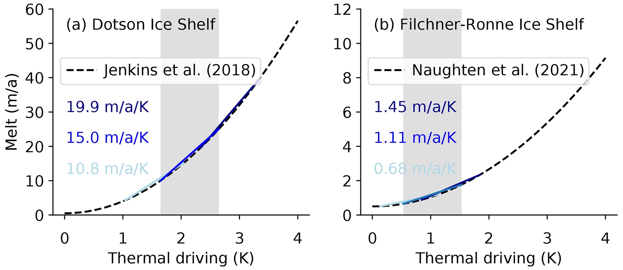
Figure 1 Sensitivities of melt rates to ocean temperature changes for (a) Dotson Ice Shelf and (b) Filchner–Ronne Ice Shelf. Thermal driving is given as temperature relative to the surface freezing point and represents properties of the water masses at depth on the continental shelf in front of the ice shelf cavity. Melt is the average melt rate over the ice shelf in metres ice equivalent per year. Dashed lines indicate estimations by Jenkins et al. (2018) and based on Naughten et al. (2021) as detailed in Appendix A1. The grey bar indicates the range over which best linear sensitivity is calculated, using present-day thermal driving for the baseline temperatures. Coloured lines and numbers show the maximum, best, and minimum linear sensitivity estimates depending on the choice of present-day baseline temperatures (see Appendix A2).

We use a temperature change of 1 K, and our best estimates of the current baseline temperatures for FRIS and the ASE are 0.53 and 1.65 ^∘C, respectively, and the minimum (FRIS: 0.13 ^∘C, ASE: 1.04 ^∘C) and maximum (FRIS: 0.84 ^∘C, ASE: 2.34 ^∘C) are taken over all values in Table A1. We test using a narrower or wider temperature change than 1 K and found that the baseline temperatures have a larger influence on the sensitivity: for example, shifting the baseline temperature by ±0.5 K gives a larger change in the sensitivity than estimating the sensitivity over a wider (2 K) or narrower (0.5 K) temperature range. Overall, we thus capture different ranges of the linearization interval by using different input temperatures (best, min, max).

By using both estimates for the Amundsen Sea and Filchner–Ronne ice shelf, we represent the sensitivity of modelled melt rates to ocean temperature changes correctly for small, warm cavities as well as cold, large cavities. Note that no observations span a wide range of temperature inputs for Filchner–Ronne, and this is why we use a recent numerical ocean model simulation that includes a switch from cold to warm conditions in the cavity (Naughten et al., 2021), with the procedure to obtain the quadratic relationship described in Appendix A1.

Resulting sensitivities of melt rates to ocean temperature changes are added as text fields in Fig. 1. For FRIS, we find a sensitivity of melt rates to ocean temperature changes between 0.7 and 1.5 $\mathrm{m}{\mathrm{a}}^{-\mathrm{1}}{\mathrm{K}}^{-\mathrm{1}}$ with the best estimate being 1.1 $\mathrm{m}{\mathrm{a}}^{-\mathrm{1}}{\mathrm{K}}^{-\mathrm{1}}$. Jenkins (1991) finds an increase from 0.6 to 2.6 m a⁻¹ for a warming by 0.6 K using plume theory, which implies a higher sensitivity of 3.3 $\mathrm{m}{\mathrm{a}}^{-\mathrm{1}}{\mathrm{K}}^{-\mathrm{1}}$ for FRIS. Hellmer et al. (2012) report that a switch from cold to warm conditions increases average melt rates from 0.2 to 4 m a⁻¹ for a warming of 2 K, which also implies a higher sensitivity of 1.9 $\mathrm{m}{\mathrm{a}}^{-\mathrm{1}}{\mathrm{K}}^{-\mathrm{1}}$. From Comeau et al. (2022, Figs. 9d and S10), we roughly estimate a melt sensitivity of 3.5 $\mathrm{m}{\mathrm{a}}^{-\mathrm{1}}{\mathrm{K}}^{-\mathrm{1}}$. The order of magnitude is in all cases comparable.

By comparison, the sensitivity of melt rates to ocean temperature changes for the ASE is higher (Fig. 1a). This might be due to the higher baseline temperatures and a larger slope of the ice shelf base (Jenkins et al., 2018). The sensitivity estimate based on the best baseline temperature of 15 $\mathrm{m}{\mathrm{a}}^{-\mathrm{1}}{\mathrm{K}}^{-\mathrm{1}}$ for Dotson Ice Shelf fits well with the estimate from Payne et al. (2007) for the Pine Island Glacier ice shelf, which is 16 $\mathrm{m}{\mathrm{a}}^{-\mathrm{1}}{\mathrm{K}}^{-\mathrm{1}}$. It is close to the initial sensitivity around 16 $\mathrm{m}{\mathrm{a}}^{-\mathrm{1}}{\mathrm{K}}^{-\mathrm{1}}$ in Seroussi et al. (2017) for Thwaites Glacier ice shelf estimated from ocean simulations with a 0.5 K temperature increase (see Fig. S5 in the Supplement of Reese et al., 2020). The sensitivity in the coupled simulation of Seroussi et al. (2017) decreases during the simulation, reaching a minimum value of 4.5 $\mathrm{m}{\mathrm{a}}^{-\mathrm{1}}{\mathrm{K}}^{-\mathrm{1}}$ and having a mean of 9 $\mathrm{m}{\mathrm{a}}^{-\mathrm{1}}{\mathrm{K}}^{-\mathrm{1}}$, which is more in line with the minimum sensitivity estimate.

2.3 Results: PICO parameter selection

We select PICO parameters such that the sensitivity of melt rates to ocean temperature changes is in line with estimates from the previous section and such that the underlying assumptions of PICO are met. In total, we optimize five pairs of parameters that span the range of different target sensitivities in FRIS and the ASE presented in the previous section (min, max, best in both regions, and combining min and max of both regions). For the parameter optimization, we conduct a parameter sweep for different values for C and ${\mathit{\gamma }}_T^{\star }$ (see Fig. 2). We select the best parameters using four criteria: (1) melting (no freezing) occurs in the first box of PICO close to the grounding line, (2) melting in the first box is larger than in the second, (3) the melt sensitivity for FRIS is close to the target from Sect. 2.2, and (4) the melt sensitivity in the ASE is close to the target from Sect. 2.2. Criteria 1 and 2 are analogous to the original parameter selection of PICO in Reese et al. (2018a), and we replace the criteria 3 and 4 of the original selection, which were to meet observed melt rates. To have the melt rates calculated by PICO replicate present-day observations (in Gt a⁻¹ from Adusumilli et al., 2020), we apply temperature corrections between −2 and 2 K to the present-day temperatures from Schmidtko et al. (2014) in each PICO basin. This is similar to the approach used by Jourdain et al. (2020, see their Sect. 4.4). We optimize temperature corrections and melt sensitivity consistently by first calculating the temperature correction for all parameter pairs $(C,{\mathit{\gamma }}_T^{\star })$ and then selecting the optimal parameter pair. With the parameter optimization, we thus obtain a set of two parameters $(C,{\mathit{\gamma }}_T^{\star })$ and temperature corrections δT_b, for each basin $b\in \mathrm{1},\mathrm{\dots }\mathrm{19}$ for each combination of target sensitivities.

Table 1 shows that indeed for all combinations of ASE and FRIS melt sensitivities, the sensitivities modelled by PICO with the respective, optimized parameters are generally in close agreement with the targets. See Tables S1 to S5 in the Supplement for the corresponding temperature corrections and comparison with observed melt rates for each parameter pair. In general, we can find temperature corrections that yield aggregated melt rates close to present-day estimates. Exceptions are basins 15 (Bellingshausen Sea) and sometimes 16 (George VI Ice Shelf), where temperature corrections of −2 K are not sufficient.

Table 1 Results of PICO parameter optimization. We optimize parameters for five combinations of sensitivity targets (selected from best, min, and max for FRIS and ASE). For each pair of target sensitivities we summarize the baseline thermal driving (T^*) used for the linearization to obtain the target sensitivity $\mathrm{d}m/\mathrm{d}{T^{*}}^{\mathrm{target}}$ for FRIS and ASE. Parameters are evaluated based on the match of modelled sensitivities $\mathrm{d}m/\mathrm{d}{T^{*}}^{\mathrm{PICO}}$ with target sensitivities. Then we give the optimized PICO parameters C and ${\mathit{\gamma }}_T^{\star }$, which are similar for all Antarctic ice shelves. For details see Sect. 2.2 and 2.3.

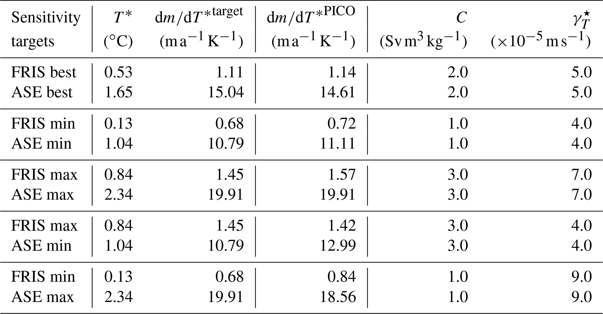
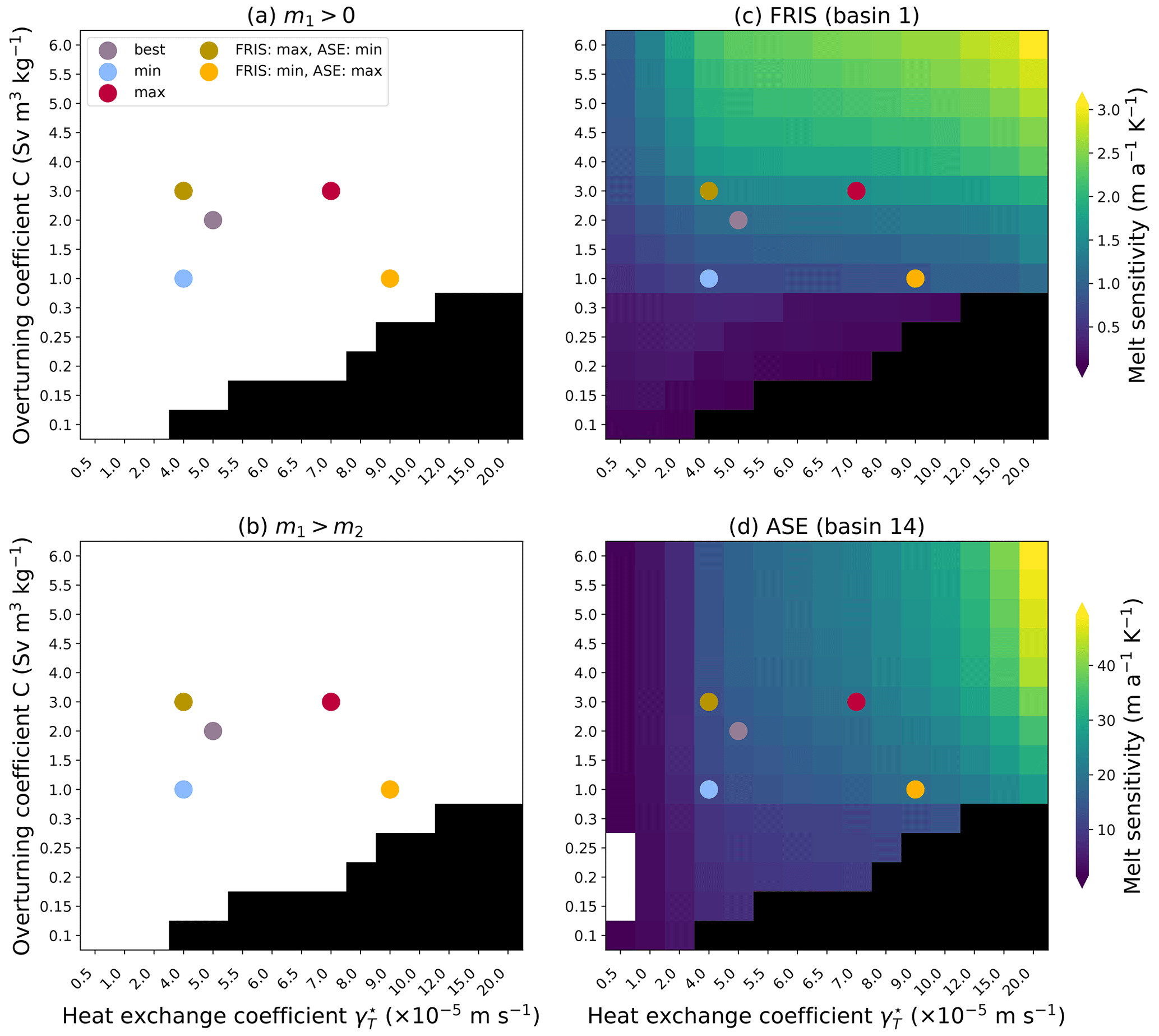
Figure 2 PICO parameter selection. Four targets are used for the optimization of the heat exchange and overturning coefficients: (a) melting and not freezing in the first box close to the grounding line, which is true in the white areas; (b) melt decreases away from the grounding line (i.e. melt rate in PICO box 1 is larger than in PICO box 2), which is true in the white coloured areas; (c) sensitivity of FRIS melt rate to ocean temperature changes; and (d) sensitivity of the ASE melt rate to ocean temperature changes, which both match best, min, max, or mixed estimates from Sect. 2.2 (indicated by dots). Note that parameter spacing on the x and y axis is not equal and that the melt sensitivities to ocean temperatures modelled by PICO that are shown in (c) and (d) have different scales. The black boxes in (c) and (d) indicate regions where the criteria (a) and (b) fail.

We find that the optimized PICO parameters range between 1 and 3 Sv m³ kg⁻¹ for C and between 4 and $\mathrm{7}\times {\mathrm{10}}^{-\mathrm{5}}$ m s⁻¹ for ${\mathit{\gamma }}_T^{\star }$, with the best estimates being 2 Sv m³ kg⁻¹ and $\mathrm{5}\times {\mathrm{10}}^{-\mathrm{5}}$ m s⁻¹, respectively. In comparison with Reese et al. (2018a), we find overall higher parameter values: the value for C from the original tuning is now valid for a low sensitivity, while in all cases the value for the heat exchange is now higher. This is in line with a rather low sensitivity of melt rates to temperature changes found in the Antarctic projections of Reese et al. (2020). In general, we find that higher sensitivities require higher parameter values. The melt sensitivity to ocean temperature changes in the large-scale ice shelves such as FRIS is dominated by the overturning coefficient, as indicated by the high value of C for high-sensitivity targets in FRIS and low-sensitivity targets in the Amundsen Sea. In the opposite case with a high-sensitivity target in the Amundsen Sea and a low-sensitivity target in FRIS, we find that for the smaller ice shelves the heat exchange coefficient ${\mathit{\gamma }}_T^{\star }$ is more important. Figure S2 shows the spatial pattern of melt rates for the min, mean, and max PICO parameters. Generally, the modelled melt rates with PICO are higher close to the grounding lines, and refreezing occurs in the large, cold cavities. Due to the box approach, melt rates are “smoothed out” and show less spatial variability than observations Adusumilli et al. (2020). In the PISM experiments presented in the rest of the article, the min, best, and max fit parameters are used.

3 Antarctic Ice Sheet simulations with PISM

In this section we describe the PISM simulations conducted using the newly optimized PICO parameters. We first describe the model and the experimental design (Sect. 3.1 and 3.2) and the ensemble of historic simulations (Sect. 3.3). Then we present results of the long-term evolution of Antarctic grounding lines under present-day climate conditions (Sect. 3.4) and analyse the large-scale reversibility (Sect. 3.5). Finally, we look into the transient, centennial evolution and test reversibility over these timescales (see Sect. 3.6).

3.1 PISM

The Parallel Ice Sheet Model (PISM; https://www.pism.io, last access: 31 July 2023; Bueler and Brown, 2009; Winkelmann et al., 2011) is an open-source ice dynamics model developed at the University of Alaska, Fairbanks, and the Potsdam Institute for Climate Impact Research. PISM is thermo-mechanically coupled and employs a hybrid of the shallow shelf approximation (SSA) and shallow ice approximation (SIA) to model ice flow. Temperatures within PISM are determined based on an energy-conserving enthalpy scheme including a thin subglacial water layer and a thermal layer in the bedrock (Aschwanden et al., 2012). A power-law relationship is applied between SSA basal sliding velocities and basal shear stress, with a Mohr–Coulomb criterion relating the yield stress to parameterized till material properties and the effective pressure of the overlaying ice on the saturated till (Bueler and van Pelt, 2015). Both the grounding line and the calving front are simulated at subgrid scale in PISM and evolve according to the physical boundary conditions. Basal friction is linearly interpolated on a sub-grid scale around the grounding line (Feldmann et al., 2014). To improve the approximation of driving stress across the grounding line, the surface gradient is calculated using centred differences of the ice thickness across the grounding line. Sub-shelf melt rates are modelled using PICO, and we use the set of optimal PICO parameters obtained with the new approach (Sect. 2). In this study we conduct an equilibrium spin-up, and as a result glacial isostatic rebound is switched off, because it would require a paleoclimate spin-up to correctly reproduce representative present-day uplift rates. We do not apply sub-shelf melt in grounded grid cells that are partially floating, and we only calve ice that extends beyond the present-day extent of the Antarctic Ice Sheet and ice shelves. Due to adaptive time stepping and usage of the superposition of the shallow ice and shallow shelf approximations, PISM is computationally efficient and capable of simulating large ensembles on multi-millennial timescales.

3.2 Experimental design and initialization

The strategy adopted to build initial present-day ice sheet configurations with PISM relies on spin-up. We account for uncertainties in model parameters by creating an ensemble of states and selecting a number of possible configurations that compare best to observations. For all ensemble members, we run historic simulations from 1850 to 2015 with the aim of reproducing current changes in ice sheet thickness.

To represent atmospheric and oceanic changes between 1850 to 2014, we use the historic forcing suggested by the Ice Sheet Model Intercomparison Project for CMIP6 (ISMIP6, Barthel et al., 2020; Seroussi et al., 2020), since no observations exist for that period in Antarctica. We apply the results from the Norwegian Earth System Model (NorESM1-M; Bentsen et al., 2013), one of the ISMIP6-suggested climate models. While the NorESM1-M simulations do not provide a perfect representation of the past climate evolution, they were found to have the smallest biases in the Southern Ocean and atmosphere (Barthel et al., 2020). Present-day ocean conditions are taken from Schmidtko et al. (2014) and then adjusted using the basin-wide temperature corrections from the PICO parameter optimization presented in Sect. 2.3. Atmospheric surface mass balance and surface temperatures are from RACMOv2.3 (1995 to 2014 averages, van Wessem et al., 2018). Note that we apply the surface mass balance from the regional climate model directly and do not calculate melting in PISM internally with a positive degree day or equivalent model. These datasets are used for present-day climate, and anomalies are applied from the NorESM1-M output, following the ISMIP6 protocol. This approach captures transient changes in the atmosphere or ocean while linearly correcting biases. Ocean and atmosphere climate conditions for the initial state in 1850 were obtained as follows: we first generate a time series of atmosphere and ocean anomalies from the modelled historic evolution that pass through zero anomalies between 1995 and 2014. We then add these anomalies to the present-day climatologies for the atmosphere and ocean, which make sure that our forcing time series passes through the present-day dataset in the period between 1995 and 2014. Finally we take the average over the first 30 years of the respective time series to arrive at historic conditions. Note that the atmospheric forcing as provided by ISMIP6 starts in 1950, and we keep it constant at the 1950 to 1980 average between 1850 and 1950. In the following, we refer to the resulting atmospheric and ocean boundary conditions as “1850” or “pre-industrial”.

Using these boundary conditions, the initial configurations are obtained as follows: starting from BedMachine ice thickness and topography (Morlighem et al., 2020), PISM is run for 400 000 years with constant geometry and climate to obtain a thermodynamic equilibrium using a 16 km spatial grid resolution. Then, an ensemble of simulations with varying model parameters is run for 25 000 years towards dynamic equilibrium at 8 km horizontal resolution using historic climate conditions roughly representing 1850. We thus make the assumption that the ice sheet was close to equilibrium in 1850, which was likely not the case. We here say that the state is in equilibrium when its rate of ice volume change is zero. Note that this is in particular true when the rates of ice thickness change are zero, i.e. when it is in steady state. Note that any tipping point that might have already been crossed due to climate changes prior to 1850 cannot be discovered with our methodology. However, starting from a state that is close to equilibrium in 1850 allows us to directly attribute any committed changes under present-day climate to the historic forcing. The simulations employ 121 vertical layers with a quadratic spacing from 13 m at the ice shelf base to 100 m towards the surface. We vary parameters related to basal sliding, in particular the till effective overburden fraction ($\mathit{\delta }\in \mathit{\{}\mathrm{1},\mathrm{1.25},\mathrm{1.5},\mathrm{1.75},\mathrm{2},\mathrm{2.25}\mathit{\}}$ %; Bueler and van Pelt, 2015), the decay rate of till water content ($C_{\mathrm{d}}\in \mathit{\{}\mathrm{7},\mathrm{10}\mathit{\}}$ mm a⁻¹; Bueler and van Pelt, 2015), and the PICO parameters (min, best, and max from Sect. 2.3). This yields 36 ensemble members to start with. From these, 15 members were discarded as they showed a collapse of the West Antarctic Ice Sheet under pre-industrial conditions during the dynamic spin-up period. After the 25 000-year equilibrium spin-up, we then use the remaining ensemble of 21 initial states to run historical simulations from 1850 to 2015, which are forced by changes in the ocean and atmosphere as described above. The corresponding changes in ocean temperature and salinity input for PICO are shown in Fig. S1.

We assess the ensemble members in 2015 using a scoring method (Albrecht et al., 2020; Reese et al., 2020) that tests the root mean square deviation to present-day ice thickness (Morlighem et al., 2020), ice stream velocities (Mouginot et al., 2019), deviations in grounded and floating area (Morlighem et al., 2020), the average distance to the observed grounding-line position (Morlighem et al., 2020), and a comparison with present-day mass losses (The IMBIE team, 2018). We focus specifically on the Amundsen region and Filchner–Ronne and Ross ice shelves by additionally evaluating each indicator for these drainage basins individually. The scoring of the present-day states is shown in Fig. B1, and all indicators are given in Table S6. We discard all ensemble members for which the modelled grounding-line positions in 2015 in the Amundsen Sea deviate on average by more than 10 km from observations (see Table S6). This further eliminates 6 members, leaving us with 15 remaining, summarized in Table 2.

While runs with PICO parameters that yield a higher sensitivity of melt rates to ocean temperature changes (i.e. max and best compared to min parameters) have better scores, no such clear distinction can be found for the decay rate of till water. The lowest possible value of δ=1.5 % yields worse scores than the other values. For this value, initial pre-industrial states that do not collapse exist only for the max PICO parameters and the best PICO parameters in combination with a higher till water decay rate (the latter was removed from the ensemble due to the large grounding-line deviations in the Amundsen Sea). This parameter sets the fraction of the effective pressure of the overlaying ice on fully saturated till to the ice overburden pressure (see Bueler and van Pelt, 2015). Lower values of this parameter yield more slippery bed conditions in particular for ice streams. Estimates from two ice streams indicate an upper limit of 0.7±0.7 % for the value of δ, mostly close to 1 % (Engelhardt and Kamb, 1997; Blankenship et al., 1987; Smith et al., 2021), which supports the use of the lowest admissible parameter values of δ=1.5 %.

We determine the equilibrium grounding-line positions by continuing the runs for another 10 000 years (in total we run thus 25 000+(2015–1850)+10 000 years). We also run control simulations with constant 1850 climate conditions parallel to all simulations to exclude any remaining trends in the initial state from influencing the results (see Fig. B2). To test whether the grounding-line positions attained after 10 000 years are reversible to their current state, we revert the climate forcing back to the 1850 conditions. We ensure that the runs are carried out for a sufficiently long time to arrive close to equilibrium. We found that 20 000 years was a sufficiently long time period for this purpose. We also test reversibility by reverting back to pre-industrial forcing after 300, 500, and 1000 years of present-day forcing. We run those simulations over the same time as the present-day continued runs until year 12015.

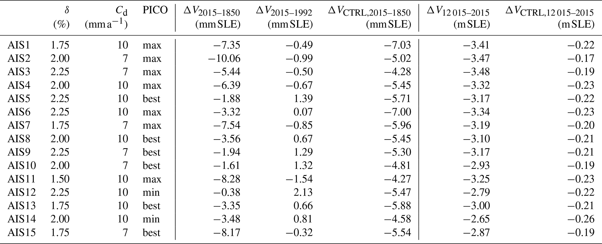
Table 2 PISM parameters of the 15 ensemble members and modelled mass changes. Runs are sorted starting with the best scores shown in Fig. B1. Given are modelled mass changes between 1992 and 2015 and between 1850 and 2015 (both relative to the control run) and drift in the control run between 1850 and 2015 in millimetres SLE for all ensemble members. This can be compared to an observed mass loss of 7.6 ± 3.9 mm SLE between 1992 and 2017 (The IMBIE team, 2018). Furthermore, we summarize committed mass loss after 10 000 years, relative to the control run, and the drift in the corresponding control run (in m SLE). Positive numbers indicate mass gain.

3.3 Results: historic simulations and present-day ice sheet configurations

Starting from quasi-equilibrium states and 1850 climate conditions, we run all 15 members of the ensemble of initial configurations from 1850 to 2015 with changes in the ocean as well as the atmosphere as described in Sect. 3.2. We refer to the initial states as “quasi-equilibrium” states, since the initial simulations have not yet reached full equilibrium, even after 25 000 years in their 1850 initial configurations (see Fig. B2; maximum rate of −1.6 m a⁻¹ ice thickness changes in single grid cells across all configurations; no spatial coherent patterns of ice thickness changes are found).

We did control runs parallel to the historic simulations and for a further 10 000 years. During the historical simulations (years 1850 to 2015), the drift is 4–7 mm SLE (sea level equivalent), and during the 10 000-year extended simulations the drift is less than 26 cm SLE (see columns “ΔV_{CTRL,2015–1850}” and “ΔV_{CTRL,12 015–2015}” in Table 2). All runs remain close to their 1850 geometrical configuration. Figure B2 shows that grounding lines move only a little for the ensemble and that rates of volume change monotonically decrease towards zero. In the following, results are presented relative to the respective control runs unless stated otherwise.

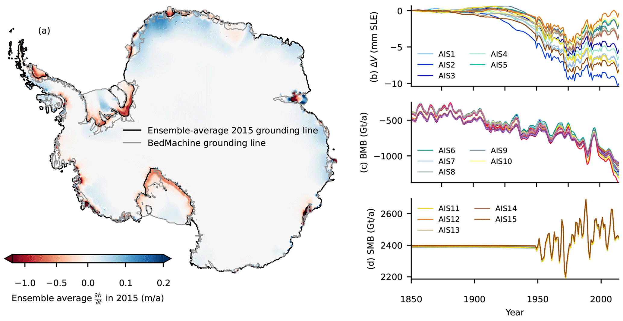
Figure 3 Historic simulations from 1850 to 2015 and present-day ice sheet configurations. Shown are (a) ensemble-average rates of ice thickness changes in 2015 (relative to control) with average grounding-line position, evolution of (b) the sea-level-relevant ice volume (in millimetres sea level equivalent, mm SLE), (c) basal mass balance of ice shelves (excluding melting in grounded regions), and (d) surface mass balance (both in gigatonnes per year).

Figure 3a presents the results at the end of these historical simulations (2015) and shows that the rates of ice thickness change averaged over all ensemble members generally resemble the observed pattern (see for example Fig. 3 in Smith et al., 2020). This is also true for individual ensemble members. In general, thinning occurs in accordance with observations in the Amundsen Sea and Bellingshausen Sea sectors, along the Antarctic Peninsula and for Totten and Moscow University ice shelves. Also in line with observations, thickening due to increased snowfall is found in the interior of the ice sheet. However, in contrast to observations, the simulations also show thinning in and upstream of Ross, Filchner–Ronne, and Amery ice shelves and in some places along Dronning Maud Land because of ocean temperature increases in these areas. This discrepancy from observations must be taken into account when interpreting the results of the long-term simulations.

Grounding-line positions and ice thickness differences to present-day observations are shown in Fig. S3 and the ensemble-average grounding-line position in Fig. 3a. All runs show grounding lines for Filchner–Ronne and Amery ice shelves that are extended seaward of observations. Furthermore, runs show a retreated grounding line on the Siple Coast of the Ross Ice Shelf, which is a problem encountered often in spin-ups as this region is close to flotation. Overall, this suggests that our results for the long-term evolution in the next section overestimate changes in the cold cavity ice shelves like Ross and FRIS.

While the pattern of thinning and thickening is overall comparable with observations, the thinning rates in the ASE sector are lower and do not extend as far inland Smith et al. (2020). As a result, simulated integrated mass losses for present-day (see column “ΔV_2015–1992” of Table 2 and Fig. 3b) are generally at the lower end of observations of 7.6±3.9 mm SLE between 1992 and 2017 (The IMBIE team, 2018). Eight out of 15 ensemble members show no mass loss or even mass gain in that period. Particularly, mass loss at Pine Island Glacier (PIG) is lower than in observations. Overall, this suggests that our results for the long-term evolution in the next section underestimate changes in the ASE. We find that mass loss is higher for PICO parameters that yield a higher sensitivity of melt rates to ocean temperature changes (max) and for lower values of the sliding parameters ($\mathit{\delta }=\mathrm{1.5},\mathrm{1.75}$ %) and till water decay rate (C_d=7) that both yield more slippery bed conditions. Such a dependency on sliding parameters, as well as a dependency on the choice of the sliding law, has also been found in previous studies (Brondex et al., 2019; Albrecht et al., 2020). Higher mass losses for the max PICO parameters in comparison to the best and min parameters are expected as those parameters yield higher changes in sub-shelf melt rates for the same historic ocean changes applied in all simulations.

Generally, sub-shelf melt increases from 1850 onward to values between 1000 and 1400 Gt a⁻¹ in 2015 (see Fig. 3c), slightly lower than observations ranging between 1173.1±148.5 Gt a⁻¹ in 1994, 1570±140 Gt a⁻¹ in 2009, and 1160 ± 150 Gt a⁻¹ in 2018 (Adusumilli et al., 2020). Differences between ensemble members occur due to different ice shelf extents in the initial states. Our historic simulations do not replicate the particularly high melt fluxes in 2009, which may be the reason why overall mass losses are at the lower end of observations. Surface mass balance varies only from 1950 onward, since no data were available beforehand, and is held constant during 1850 to 1950 (see Fig. 3d). It is similar for all ensemble members since the maximum ice extent is pre-defined based on BedMachine Antarctica, and the integrated surface mass balance is hence similar for all members.

3.4 Results: long-term equilibrium grounding-line positions under present-day climate conditions

We investigate the long-term evolution of present-day Antarctic grounding lines by keeping the present-day climatology constant following the historic simulation and letting the ice sheet state evolve towards a new equilibrium for 10 000 years. Note that 10 000 years might not be sufficient to reach negligible changes in ice volume and grounding line, but we get a clear indication of what such an equilibrium state might look like. We then investigate whether the grounding lines remain close to their currently observed position or if they retreat substantially.

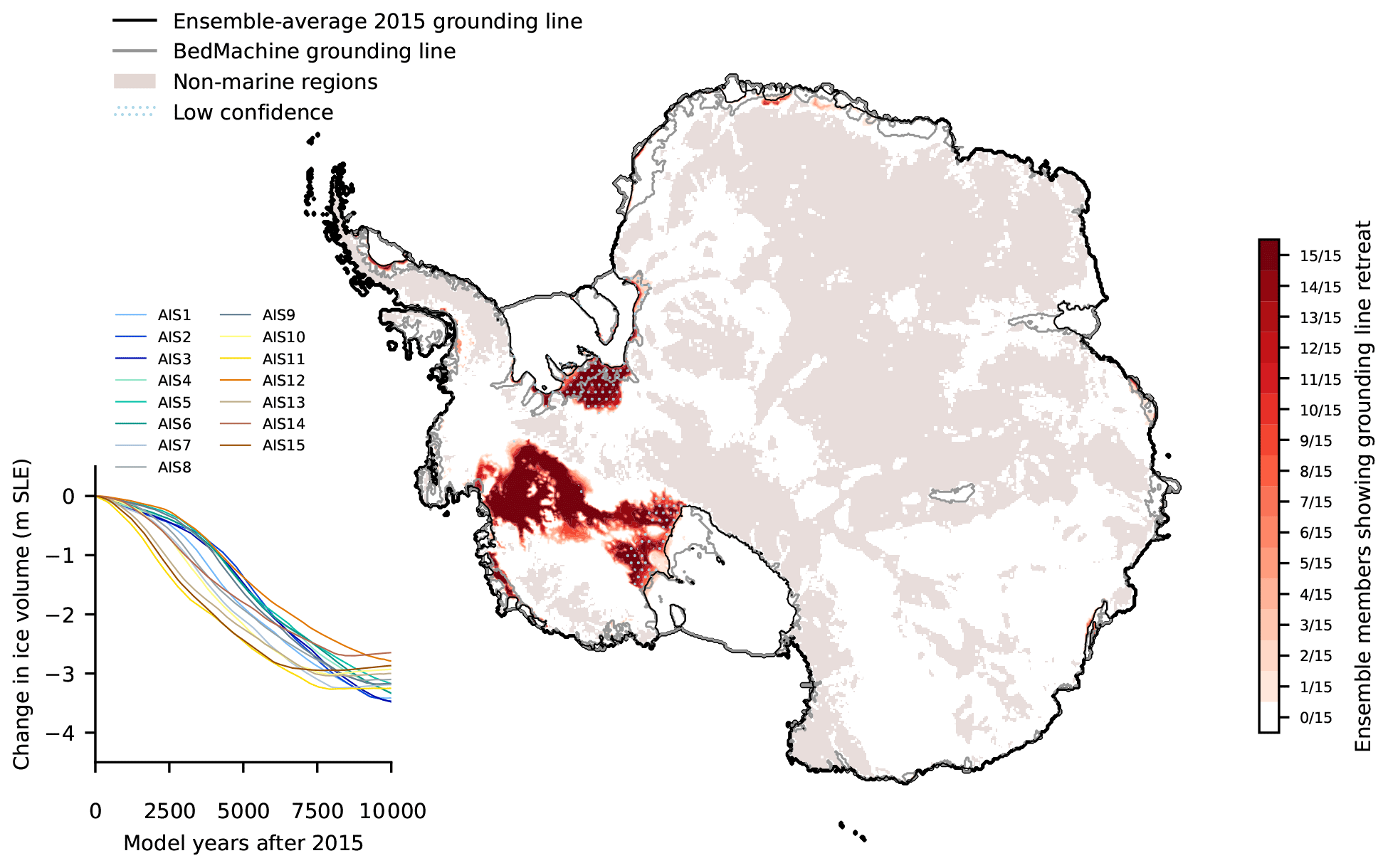
Figure 4 Long-term evolution of present-day Antarctic grounding lines under constant present-day climate conditions. Starting in present day after the historic forcing from 1850 to 2015, simulations are continued with constant present-day climate for 10 000 years. Red colours show regions over which the grounding line retreats. The darker the red, the more model configurations show grounding-line retreat over the respective region (retreat is plotted in comparison to a control simulation). Black contour shows ensemble-average initial grounding-line position in 2015. Inset shows the evolution of sea-level-relevant ice volume for all ensemble members (m SLE, metres sea level equivalent, relative to the drift in the initial state over that period). Dots on retreat areas indicate regions in which present-day modelled thinning is inconsistent with observations (namely for Filchner–Ronne and Ross ice shelves). Light brown indicates bedrock above present-day sea level; white areas indicate bedrock below sea level.

Figure 4 shows that the grounding lines of the present-day configurations retreat substantially in the marine regions of West Antarctica over the 10 000 years with constant climate conditions. Overall, mass loss ranges between 2.7 m and 3.5 m SLE (see column “ΔV_{12 015–2015}” of Table 2) with the maximum rates of ice loss over the 10 000 years ranging between 0.7 mm a⁻¹ for AIS14 and 0.9 mm a⁻¹ sea-level-equivalent ice loss for AIS11. For comparison, the drift in the historic initial states over this period is less than 30 cm. Note that some states are still losing ice at the end of the simulation time, and thus grounding lines might not have converged fully to a new equilibrium position (see Fig. S4). This is most prominent for AIS1–AIS6 and AIS12, which mostly show continued mass loss in Pine Island (except for AIS6, which shows no retreat of Pine Island Glacier but further retreat in the region connecting Thwaites and Ross).

Grounding-line retreat and the associated loss of large parts of the marine basins are found in the ASE sector, upstream of Thwaites Glacier, and in some cases upstream of Pine Island Glacier. Grounding lines for the individual ensemble members are shown in Fig. S4. All states except for AIS6, AIS10, and AIS15 show partial (AIS7) or substantial retreat of Pine Island Glacier. For a large number of these states this connects to the retreat in Thwaites (AIS1, AIS2, AIS3, AIS4, AIS5, AIS9, AIS11, AIS12). As discussed in the previous section, Pine Island Glacier's grounding line is too far downstream (around 50 km) of present day in all ensemble members, and modelled present-day thinning rates are too low in comparison with current observations. We find some retreat in Smith, Kohler, and Pope glaciers, which does, however, not extend very far upstream of the present-day grounding-line positions.

We find that all ensemble members retreat in the Robin subglacial basin and towards the ice rumples of the Ronne Ice Shelf that were grounded in the initial states, although it is floating in observations. All runs show retreat that continues beyond present-day grounding-line positions. As we discussed in the previous section, this region shows thinning after the historic simulation that is not in line with observations. Grounding lines retreat for almost all members of the ensemble on the Siple Coast of the Ross Ice Shelf in the 10 000 years. Similar to FRIS, the historic runs show thinning in this region which is not compatible with observations. All runs except AIS6 show a connection between Thwaites Glacier and the Ross Ice Shelf. A retreat of Thwaites can also indirectly trigger retreat in Ross as discussed for an idealized system in Feldmann and Levermann (2015b). Further work is required for both ice shelves with large, cold cavities to understand current climate forcing and committed retreat. In all other regions of Antarctica we find only small retreat of grounding lines (less than 25 km in the 10 000 years).

3.5 Results: (ir)reversibility of large-scale retreat

To test whether large-scale retreat after 10 000 years (see previous section) is (ir)reversible, we revert climate forcing back to pre-industrial conditions and extend the simulations for another 20 000 years. Reversibility experiments that we did at earlier points in time to narrow down the onset of irreversible retreat are discussed in Sect. 3.6. Figure 5a summarizes reversibility for all runs; individual results are shown in Fig. S5, which also shows that rates of ice thickness change at the end of the reversibility runs are small enough to consider the grounding lines close to equilibrium. We find that retreat in Thwaites Glacier shows overall no reversibility with the reversed grounding line close to the collapsed one in all simulations. Pine Island Glacier shows reversibility of the grounding line to their 2015 positions in some simulations (AIS8, AIS9, AIS12), the grounding-line advancing to intermediate locations in some (AIS1, AIS2, AIS3, AIS4), and no advance (AIS5, AIS11, AIS13) or continued retreat (AIS14) in others. This could indicate that several regions of irreversible retreat (and tipping points) exist, in line with Rosier et al. (2021), and that in some cases the reduction in the forcing is sufficient to “jump” back across all tipping points to the initial grounding-line position, while in others not all or none of the tipping points can be reversed. In contrast, FRIS shows clear reversibility, where the grounding line re-advances to almost its present-day or historic position in the initial configurations in all cases. The western Siple Coast in Ross Ice Shelf also shows reversibility, with the grounding line reaching a position slightly upstream of the modelled present-day location once the connection to Thwaites has become grounded. Where the ice shelves remain connected, the grounding lines in Ross do not reverse or re-advance to intermediate positions. The eastern Siple Coast shows irreversible retreat in most cases and remains retreated.

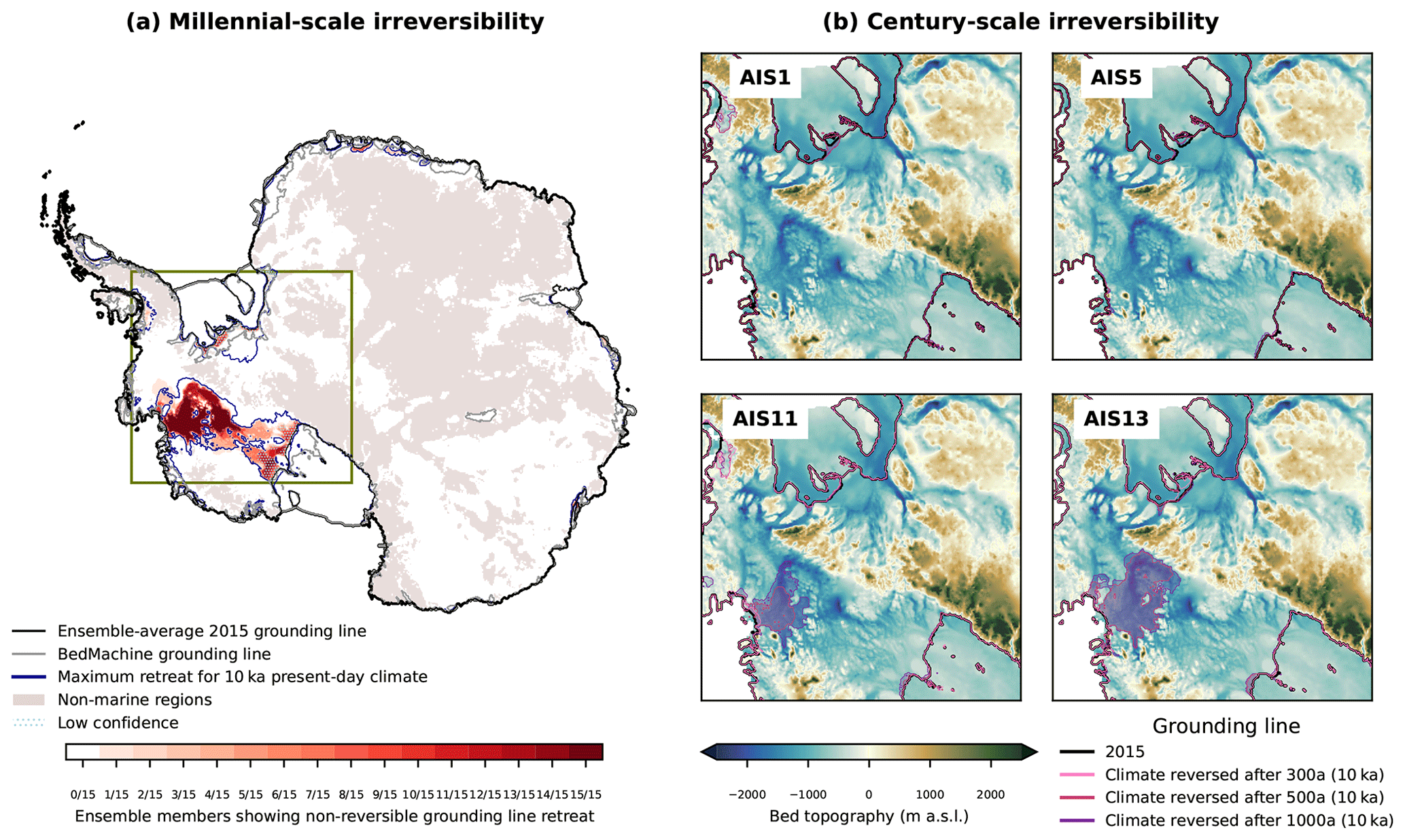
Figure 5 Reversibility experiments of large-scale retreat. (a) Millennial-scale experiments. Red areas show regions that remain ungrounded after 20 000 years of (reverted) historical climate following the 10 000 years of constant present-day climate that caused grounding lines to retreat (see Fig. 4). The maximum extent of grounding-line retreat after 10 000 years constant climate is shown in blue. The darker the red, the more potential present-day configurations show irreversible grounding-line retreat over the respective region. Other labels as in Fig. 4. Box shows the zoom of the right panels. (b) Centennial-scale experiments. Four present-day configurations of Antarctica, with their 2015 grounding lines shown in black, are integrated forward under constant present-day climate. When reversing the climate to historic conditions after 300, 500, and 1000 years in the simulations, grounding lines evolve to the locations shown in the map (positions in year 12015); differences to present-day grounding lines are indicated by shading. The base map shows the bed topography from BedMachine (Morlighem et al., 2020). We here show the best ensemble member (AIS1), the best ensemble member for “mean” PICO parameters (AIS5), and two examples, AIS11 and AIS13, that show centennial onset of irreversible retreat.

3.6 Results: transient evolution on centennial timescales

We furthermore test the reversibility at earlier stages of the simulation and analyse the ice sheet evolution over the initial 300 years. This is shown for four examples with different behaviour in Fig. 5b; all reversibility runs are shown in Fig. S4. We test reversing the climate conditions to pre-industrial conditions after 300, 500, and 1000 years of constant present-day conditions and extend the runs until year 12015. Doing so allows us to narrow down the onset of irreversible retreat. Until year 300, none of our simulations show irreversible retreat, since when reversing the forcing back to pre-industrial conditions, the grounding lines stay in their location or re-advance to their pre-industrial positions. However, when reversing after 500 years, AIS11 shows continued retreat of Thwaites Glacier, and AIS13 shows continued retreat of Thwaites and Pine Island glaciers. The same is true for another initial configuration (AIS15). When reversing after 1000 years, additionally AIS14 shows continued retreat. The continued retreat indicates the onset of irreversible retreat prior to the respective time. This is also visible from the evolution of the ice volume (see first column of Fig. 6). To summarize, we find that $\mathrm{3}/\mathrm{15}$ of ensemble members show an onset of irreversible retreat between 300 and 500 years of constant present-day climate conditions, and $\mathrm{11}/\mathrm{15}$ show no onset of irreversible retreat within 1000 years. This shows that the timescale at which irreversible retreat starts is dependent on the model parameters of the initial configuration.

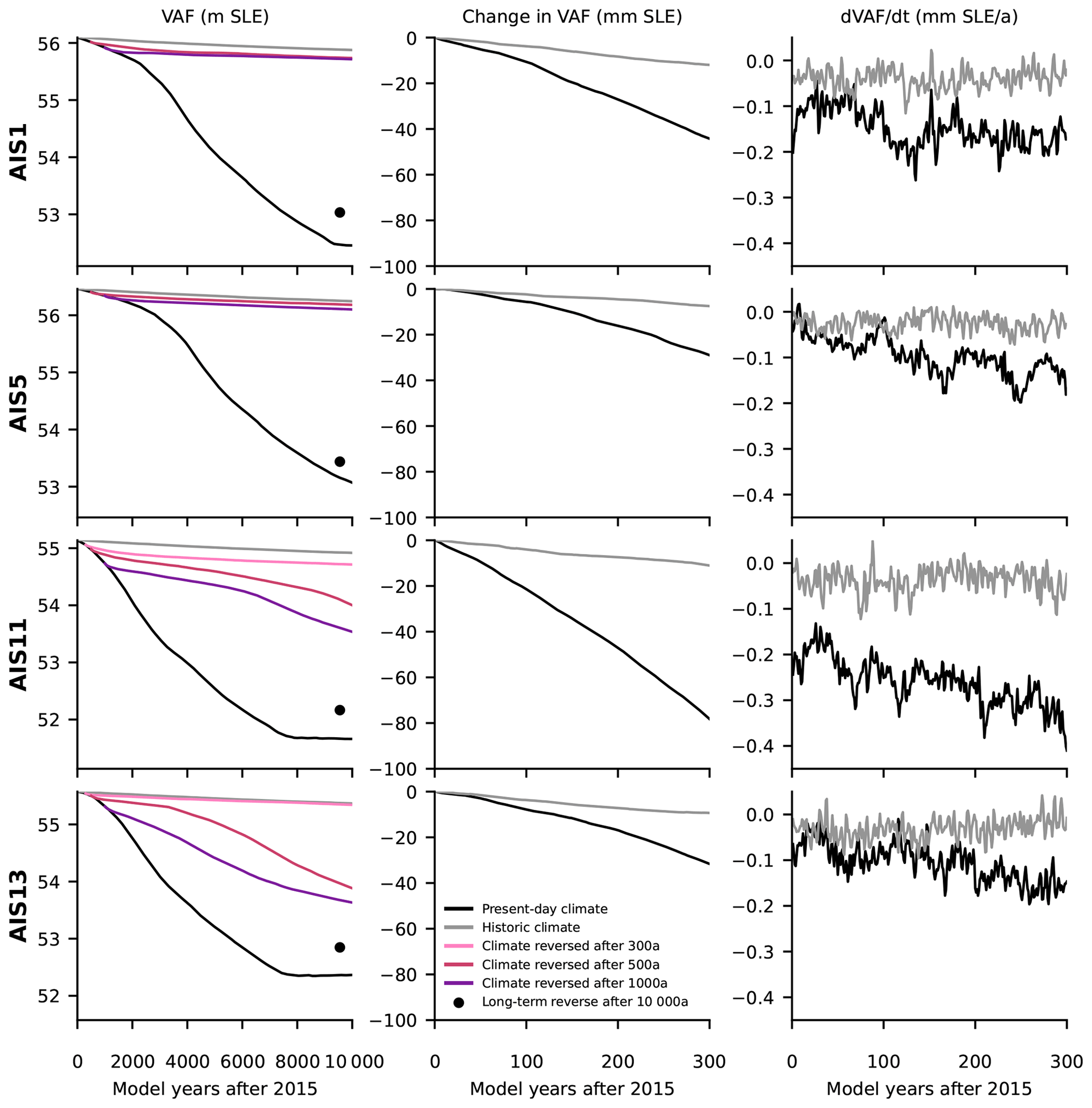
Figure 6 Evolution of selected ensemble members over 10 000 and 300 years. Shown are the sea-level-relevant ice volume over 10 000 years (left panels), its change over 300 years (middle panels), and the rate of volume change over 300 years (right panels). We show the evolution for the best ensemble member (AIS1), the best ensemble member for “mean” PICO parameters (AIS5), and AIS11 and AIS13, two members that show centennial onset of irreversible retreat. Dots in the left panels show the volume above flotation after 20 000 years of reversing to pre-industrial conditions following the 10 000 years of present-day climate conditions.

In addition, we analyse the rates of ice loss and the total ice loss. In the first 300 years of the simulations with constant present-day climate starting in 2015, we find an increasing rate of volume loss with a maximum rate of 0.4 mm a⁻¹, leading to 8 cm of sea-level-equivalent mass loss (see Fig. 6).

4 Discussion

In the following sections, we discuss the optimization of PICO parameters (see Sect. 4.1) and the PISM experiments (see Sect. 4.2). Based on these, we then discuss tipping in Antarctica with respect to MISI in Sect. 4.3.

4.1 PICO parameter selection

In this paper we have selected PICO parameters such that the sensitivity of sub-shelf melt rates to ocean temperature changes in FRIS and for the ASE ice shelves matches with independent estimates. We applied temperature changes between −2 and 2 K to obtain the aggregated observed melt rates in each basin of PICO. This range spans almost the entire variation of ocean temperatures observed in the Southern Ocean, and large temperature corrections could point to missing assumptions in the melt calculation. However, we are interested here in the ice sheet response, and for the ice sheet it is important to have the correct present-day melt rates as well as the correct increase in melt rates with ocean temperature changes, which is achieved by this method. Note that using temperature corrections makes our approach independent of the input temperatures and thus subjective choices of how to calculate “far-field” input.

Our approach yields different parameters to those of previous studies (Reese et al., 2018a, 2020) and to those of a recent study (with ${\mathit{\gamma }}_T^{\star }=\mathrm{0.39}\times {\mathrm{10}}^{-\mathrm{5}}$ m s⁻¹ and C=20.5 Sv m kg⁻¹; Burgard et al., 2022), which optimized parameters to match with model simulations of NEMO (Nucleus for European Modelling of the Ocean) under present-day conditions. Earlier studies only used present-day melt rates as targets, not the sensitivity of melt rates, which is arguably more important for perturbation experiments or projections. While the NEMO simulations did include variability in the ocean input, one reason for the differences in the parameters could be that the NEMO simulations did not include a similarly strong increase in melting of FRIS, which we use here explicitly for parameter optimization. Furthermore, here we concentrate on those two regions which are classified as “warm and small cavities” and as “cold and large cavities”, respectively, while Burgard et al. (2022) optimized parameters for all major ice shelves around Antarctica. Our parameters hence might not be suited for other ice shelves, in particular ice shelves in different regimes, e.g. “small and cold cavities”. Note that the grounded ice streams that drain these types of ice shelves might not contribute substantially to sea level in the future. For an idealized cavity, Favier et al. (2019) compared PICO and other melt parameterizations to a coupled model and found that modelled ice mass loss was comparable.

We conclude that the parameter selection for PICO should be adapted to the aim of the study in which they are applied. Since in our study we find most changes for the ASE sector and the large Filchner–Ronne and Ross ice shelves, we think that our parameter selection procedure with particular focus on these regions is appropriate. The way the parameters are selected, by linearizing between present-day ocean temperatures and +1 K increased conditions, also makes this method applicable for conducting sea level projections.

4.2 PISM experiments

Here we use a suite of PISM simulations that apply changes from 1850 to 2015 and then keep the present-day climate constant for 10 000 years to address the question of committed retreat under present-day climate conditions. In all simulations we reverse the forcing to 1850 conditions to test for reversibility of the grounding lines. One caveat of the applied methodology is that we rely on the historic forcing by the general circulation model NorESM1-M (Bentsen et al., 2013), which was selected by ISMIP6 due to its best performance around Antarctica (Barthel et al., 2020), but it might incorrectly represent trends in the atmosphere and ocean in some places since coarse-resolution climate models cannot fully resolve the important processes on the continental shelf. Furthermore, PICO coarsely samples water masses north of the ice shelves at the depth of the continental shelf, and the CMIP forcing is directly, without any modifications, transferred from offshore into the ice shelf cavity. This representation of the ocean forcing might explain why we find thinning in the Weddell and Ross seas through the historic model simulations, while observations indicate none of these (Smith et al., 2020), and, in addition, why all runs show grounding lines for Filchner–Ronne and Amery ice shelves that are located seaward of observations. The committed specific patterns of retreat simulated in these regions must be interpreted with caution. However, we can use this modelled retreat to test for reversibility, and we find that large-scale retreat of the grounding lines of the Filchner–Ronne Ice Shelf and the western Siple Coast of the Ross Ice Shelf is reversible if they are allowed to regrow to their initial geometry. Whether Ross and FRIS could become substantial contributors to sea level rise in the future, or show tipping behaviour in the ocean (Hellmer et al., 2017; Naughten et al., 2021), is an active field of research. Understanding the committed evolution of both systems at present and under future warming in a coupled configuration would hence be of great interest.

On the other hand, our simulations underestimate present-day mass loss in the ASE sector. This might be explained by ocean forcing that is too weak in comparison to present day and other factors, like the horizontal resolution of 8 km in the model simulations, snowfall increases that are too high, the exclusion of calving and damage from the simulations, or the choice of the friction law. Generally ocean forcing in the Amundsen Sea is a complicated process (Jenkins et al., 2016; Holland et al., 2019), and more work is needed to understand its effect on the stability regime. We keep present-day climate conditions constant, but substantial decadal variability is observed in particular in the Amundsen and Bellingshausen seas (Jenkins et al., 2018), which is known to influence numerical results (Hoffman et al., 2019). Similarly, the biases in the surface mass balance field and their modelled evolution can affect the results. Improved data on the present-day forcing, and its variability, would be required to further investigate the commitment of the WAIS collapse. Our experiments rely on PICO for providing sub-shelf melt rates and RACMO for providing the surface mass balance field. Discrepancies from observations will influence the results, and it would hence be interesting in future work to analyse the influence of alternative melt parameterizations, such as a quadratic parameterization and alternative surface mass balance fields on the timing and reversibility of grounding-line retreat.

Since there is still a small drift in our simulations after 10 000 years, we did not fully identify the equilibrium grounding-line position that the 2015 grounding lines in our model are attracted to. All results are hence given with reference to this time frame, but they allow us to analyse the evolution of the system over a rather long period of time. Similar caveats apply for the reversibility simulations, which we maximally ran over 20 000 years to reduce drift in the final states. In addition, our experiments focus on reversibility of large-scale retreat. Smaller events of irreversible retreat might occur that are not distinguishable in the large-scale picture (see Rosier et al., 2021).

Here we used an ensemble approach to better understand the influence of ice sheet model parameters on the sensitivity of present-day Antarctic grounding lines. Due to computational constraints, we could not explore the full parameter space. Moreover, an important mitigating factor for MISI is relative sea level change at the grounding line that can be induced through gravity changes (Gomez et al., 2010) as well as glacial isostatic rebound (Gomez et al., 2015; Whitehouse et al., 2019). These feedbacks make grounding lines less prone to instability. For creating consistent initial states with the two other models in the companion paper that all include as similar model physics as possible and due to the equilibrium spin-up procedure chosen here, those feedbacks are not accounted for in the PISM experiments. Also for the first reason, we do not apply calving except for prescribing the ice front at its present location or adjustments of the surface mass balance to surface elevation changes. Our representation of melting relies on a parameterization that is less sophisticated than coupled ice–ocean models (e.g. Seroussi et al., 2017). It also does not include the enhancing effect of subglacial discharge on sub-shelf melt rates (Wei et al., 2020; Nakayama et al., 2021). Not considered in our experiments are feedbacks between the ice sheet and the ocean: increasing meltwater input into the ocean has been shown to generally reduce air and ocean temperatures in the Southern Hemisphere (Swingedouw et al., 2008) while trapping warmer waters below the surface close to the continent, leading to enhanced sub-shelf melting from Antarctica (Bronselaer et al., 2018; Golledge et al., 2019). Note that these modelling choices make it possible to analyse the existence of MISI independently from the above-mentioned positive or negative feedback mechanisms. Feedback mechanisms that are included in the simulations are thermomechanical feedbacks between sliding, saturation of the till, englacial strain rates, and friction since we let the ice enthalpy and basal till water content evolve in the simulations. Note that calving could influence the stability regime substantially (Haseloff and Sergienko, 2018). Since calving upstream of the current ice front would mostly reduce ice shelf buttressing or not impact it, we would expect that including this process would not affect our finding of large-scale irreversible retreat in the Amundsen Sea under current climate forcing. Results on reversible retreat in our simulations could be affected by more disruptive calving. The way melting is applied at partially floating grid cells is known to influence the results (Seroussi and Morlighem, 2018), and thus we do not apply melting in grounded cells that are partially floating. A study with a higher resolution of individual regions could help to understand the effect of potentially prohibiting melting over important regions close to the grounding line.

We start the historic simulations from an equilibrium state in 1850, which does not include the paleoclimate history of the Antarctic Ice Sheet. That the climate history is not included in modelled temperatures will influence in particular inland ice velocities in slower-flowing regions and thus the sensitivity of the grounding line to large-scale retreat. Furthermore, it means that any grounding-line retreat that was committed before 1850 cannot be considered in this analysis. However, this approach makes it possible for us to perform a clearly defined analysis of the effect of the recent ice sheet history on its committed grounding-line evolution. In their model simulation of the evolution of the Antarctic Ice Sheet since the last interglacial, Golledge et al. (2021) find the WAIS to retreat under current climate conditions. Their simulation includes past-climate influence on englacial temperatures, glacial isostatic adjustment, and calving and is hence complementary to our approach. They do not test for irreversibility. It would be interesting, as a next step, to analyse the remnant influence of past glacial cycles and interglacial climates on the currently committed grounding-line retreat (and reversibility of retreat) in more detail.

Finally, we compare our results to previous studies. The timescales over which the WAIS collapses in our simulations are on the order of thousands of years. This timescale is similar to other studies that analyse tipping processes (Garbe et al., 2020; Rosier et al., 2021; Feldmann and Levermann, 2015a; Mengel and Levermann, 2014). The onset of irreversible retreat occurs at different times in the simulations, showing that further work is required to better understand the likelihood of the onset of irreversible retreat in the future. It is known that stronger forcing can increase the rates of mass loss substantially and shorten timescales. For example, following a complete removal of ice shelves, the WAIS was found to collapse within a few centuries (Sun et al., 2020). The volume of committed ice loss we find is similar to previous studies. For example, Golledge et al. (2021) suggest a committed loss of up to 4 m SLE. The maximum mass loss over the next 300 years under constant present-day climate forcing is 0.4 mm a⁻¹, which is in line with present-day rates (The IMBIE team, 2018).

4.3 Has the (West) Antarctic Ice Sheet already tipped?

To discuss our modelling results in the context of tipping, here we first introduce relevant concepts (see Sect. 4.3.1). Then we discuss the implications of the accompanying paper (Hill et al., 2023) as well as our simulations for the potential qualitative states that Antarctic ice streams or glaciers could be in with respect to MISI (see Sect. 4.3.2), and we discuss this classification (see Sect. 4.3.3). Note that the terminology used here for nonlinear systems is based on Strogatz (2018).

4.3.1 Theoretical framing

MISI occurs when a positive feedback, where retreat of the grounding line increases the ice flow across the grounding line and this in turn causes further retreat, is at play. In a simplified system, assuming a laterally uniform ice sheet or ice stream with constant bed properties, small bed gradients, and ice rheology, it was shown that ice flow across the grounding line is a function of the local ice thickness (which is linked through the flotation criterion to the bed topography) and that the stability can thus, due to the positive feedback, be determined from bed slope (stable on prograde, unstable on retrograde bed slopes; Schoof, 2007, 2012). However, conditions that apply to real systems are known to be more complicated. In the presence of buttressing ice shelves, it is possible that MISI is suppressed (Gudmundsson et al., 2012; Haseloff and Sergienko, 2018; Pegler, 2018). In the absence of buttressing, it was found that also non-negligible bed conditions (Sergienko and Wingham, 2022) or a specific distribution of the basal friction parameter (Brondex et al., 2017) can allow for stable steady-state grounding lines on retrograde sloping beds. Numerical modelling is hence required to assess the existence and conditions under which MISI occurs. The potential for irreversible grounding-line retreat in regions upstream of present-day grounding lines has been shown in numerical simulations for the whole Antarctic Ice Sheet (Garbe et al., 2020), the West Antarctic Ice Sheet (Feldmann and Levermann, 2015a), and the Wilkes subglacial basin in East Antarctica (Mengel and Levermann, 2014) and using high-resolution modelling with an in-depth tipping analysis for Pine Island Glacier in the ASE sector (Rosier et al., 2021). The existence of irreversible retreat for other grounding lines requires further investigation.

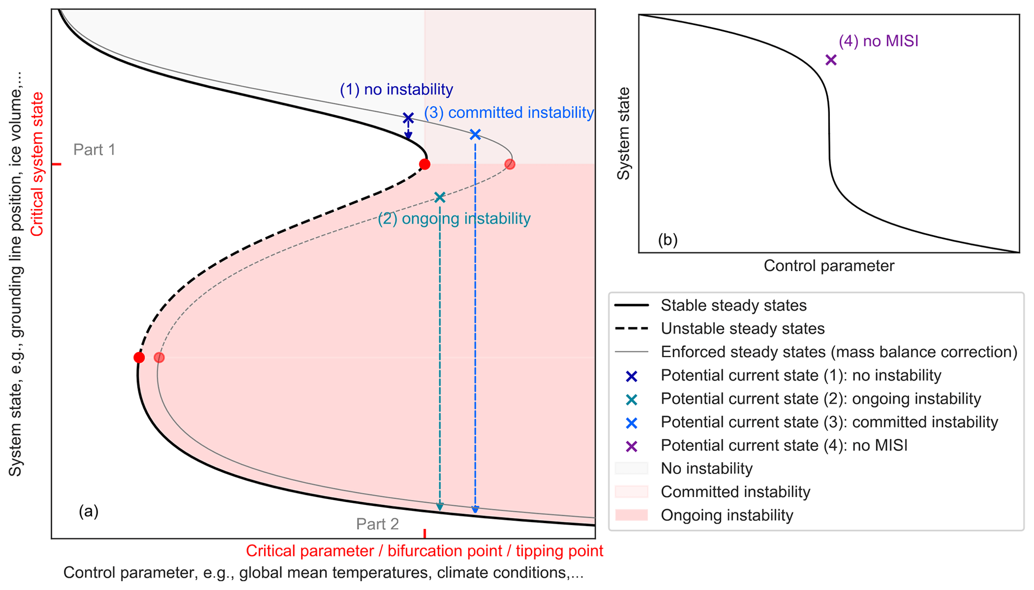
Figure 7 Schematic of potential present-day states of Antarctic grounding lines with respect to MISI. Illustrated is (a) a schematic bifurcation diagram for the marine ice sheet instability (MISI) and (b) a schematic diagram illustrating a reversible system, both represented by a system state and a control parameter and both showing potential for large-scale transitions. Black curve shows underlying steady system states (solid for stable, dashed for unstable). Bifurcations are indicated by red dots with their critical control parameter (also referred to as bifurcation or tipping point) shown on the x axis and their corresponding critical system state indicated on the y axis. If MISI exists (a), the current, transient grounding line (indicated by crosses) might be at three qualitatively different locations relative to the steady-state curve and the tipping point. If no MISI exists (b), large-scale changes in the system state are reversible. The companion paper, Part 1 (Hill et al., 2023), assesses whether the grounding line is currently undergoing MISI, by enforcing a steady state using a mass balance correction (grey curve). In this paper, Part 2, we analyse the long-term evolution of the grounding lines (indicated by arrows relative to the black curves) and their reversibility, i.e. whether large-scale retreat is committed under constant climate forcing and, if so, whether this retreat is reversible.

MISI gives rise to hysteresis behaviour (Schoof, 2007), which can be visualized in a bifurcation diagram showing the system state, e.g. current location of the grounding line, with respect to the relevant control parameter, e.g. climate forcing in the atmosphere and ocean (see Fig. 7). Hysteresis means that, over a range of control parameter values, several possible steady system states exist, and thus the (evolution of the) current system state depends on its history. Those steady system states, or grounding-line positions, can be stable or unstable, depending on whether a small-amplitude perturbation to the system is dampened (stable) or amplified (unstable) so that the system evolves back to its original steady state or away from it. At the threshold value of the control parameter, a stable and an unstable branch merge. If the control parameter is moved beyond that (bifurcation/tipping) point, the system will engage in an irreversible transition towards the only existing stable system state. Moving the control parameter across a tipping point is how tipping in marine ice sheets is generally thought to occur (this is called bifurcation-induced tipping; alternative ways of tipping are discussed, for example, in Vanselow et al., 2022). Such a transition is called “irreversible”, since reverting back to the original system state requires the control parameter to be reduced substantially below the tipping point value until a second tipping point is crossed and the system irreversibly changes back to the first state. See Rosier et al. (2021) for a more detailed discussion.

We hypothesize that glaciers, ice streams, and marine basins of the Antarctic Ice Sheet that undergo MISI show “slow-onset” tipping (Ritchie et al., 2021). This would mean that it is possible to have a temporary overshoot of the control parameter, i.e. climate conditions, above the tipping point without forcing the grounding lines to enter irreversible retreat, i.e. WAIS collapse. Such a mechanism has been described for other systems as affording “borrowed time”, in which it is possible to revert to previous conditions before the undesirable system state locks in (Hughes et al., 2013). It is plausible since, under very slowly increasing control parameters in quasi-steady experiments, the ice sheet's system state was found to evolve above the equilibrium curve (see Garbe et al., 2020, and Rosier et al., 2021).

An Antarctic ice stream whose grounding line has been forced to retreat could hence be in one of the four qualitative positions in terms of MISI (see Fig. 7):

1. No instability. The ice stream has one (or several) tipping point (points) related to MISI, but the tipping points have not been crossed. Letting the grounding line evolve with the control parameter (climate) kept constant, it would reach a stable steady state not too far inland from its current position, i.e. remain on the upper stable branch (following the dark-blue arrow in Fig. 7a). This state is not tipped.

2. Ongoing instability. The grounding line is currently undergoing irreversible retreat after crossing a tipping point related to MISI. When evolving this system forward under constant climate conditions, the grounding line retreats further until it reaches a new stable steady-state branch (following the turquoise arrow in Fig. 7a). This retreat is irreversible; i.e. reducing the climate conditions back to the pre-tipping value is not sufficient to stop the retreat. Such a state is considered to be tipped.

3. Committed tipping. The ice stream has a tipping point related to MISI, and the control parameter has crossed the corresponding tipping point, but the grounding line has not yet engaged in irreversible retreat. Under constant climate conditions, the grounding line will eventually enter irreversible retreat (following the light-blue arrow in Fig. 7a), but this retreat could still be prevented by reducing the control parameter below its critical value. Such a state is considered to be “not tipped yet”.

4. No MISI. The ice stream has no tipping point related to MISI. The system might show large-scale changes for small changes in the control parameter, but these are reversible when the control parameter is reversed (Fig. 7b).

4.3.2 Potential states of present-day Antarctic grounding lines with respect to MISI

The numerical analysis of our companion paper (Hill et al., 2023) shows that MISI is likely not occurring at any of the Antarctic grounding lines at present. In that paper, a balance approach is used by which the surface mass balance is modified so that the current Antarctic grounding lines are in steady state (schematically indicated by the grey curve in Fig. 7a). Then, their stability is tested in a numerical stability analysis. A stable steady state was found for all grounding lines with respect to the modified surface mass balance, which indicates that the grounding lines are likely not undergoing MISI in their current positions or that no MISI exists. This can be interpreted as case 2 being likely untrue. The present paper investigates the question of whether the current Antarctic grounding lines are more likely to represent case 1, 3, or 4.

We first discuss the ASE sector. Our reversibility experiments show that MISI exists for Thwaites Glacier and, similarly, for Pine Island Glacier, which is in line with previous findings (Favier et al., 2014; Feldmann and Levermann, 2015a; Rosier et al., 2021) and excludes case 4. That the “overshoot” state 3 indeed exists for Antarctic grounding lines becomes clear from our experiments: our Antarctic configurations show a long-term irreversible collapse in Thwaites Glacier (i.e. that it could be in state 2 or 3 and not in 1), and when we reverse the forcing after the historic simulation until 2015 and another 300 years of constant present-day climate back to the 1850 climate conditions, all runs show reversibility, excluding case 2 in line with Hill et al. (2023). The current grounding line of Thwaites could hence indeed be the state of case 3, and the collapse can still be reversed in present day. We have similar findings for PIG, although overall retreat is less pronounced.

We now discuss the Filchner–Ronne and Ross ice shelves. Hill et al. (2023) hint at state 2 being unlikely, in line with our reversibility experiments showing no continued retreat in these regions when reversing the climate to pre-industrial conditions after 300 years. Our long-term, constant-climate experiments expose a large part of the marine basins upstream of both ice shelves; this is likely unrealistic as discussed in Sect. 4.2. However, it allows one to test for reversibility in the case of such large-scale retreat. In our experiments, grounding lines in Filchner–Ronne and Ross ice shelves are in most areas reversible, indicating them to be in state 4 and not in 1, 2, or 3. However, hysteresis could be possible, but the climate forcing changes so much in the experiments that it “jumps” over the loop; i.e. we cannot exclude the other states on the basis of our experiments. Reversibility, or case 4, would be consistent with numerical modelling and theoretical findings of stable grounding-line position on retrograde sloping beds in the presence of buttressing, as discussed in Sect. 4.3.1, since grounding lines in Filchner–Ronne and Ross ice shelves were reported to show strong buttressing (Reese et al., 2018c).

Other grounding lines show no large-scale retreat in our experiments. They are thus neither in state 2 nor 3 according to our simulations. Distinguishing whether they are in state 1 or 4 is not possible in our experiments, and more work would be needed to understand their potential for irreversible retreat.

4.3.3 Discussion of classification of potential states

Our classification of Antarctic grounding lines (Sect. 4.3.1 and 4.3.2) is based on the assumption that steady-state positions exist. Since ice dynamics are also influenced by thermodynamics, oscillatory or limit cycle behaviour is also possible. In this case the system would not settle on one stable steady state if ran forward under constant conditions but on a closed, oscillatory attractor (e.g. Feldmann and Levermann, 2017). However, a previous study that included thermodynamics (Garbe et al., 2020) generally showed hysteresis behaviour for Antarctica on a broad scale, so we think that making this assumption is appropriate here. Similarly, other previous studies assessing the long-term (thousands to millions of years) hysteresis behaviour of the Antarctic Ice Sheet also show steady-state behaviour, with cyclic behaviour only simulated in response to a cyclic external forcing (e.g. insolation changes on orbital timescales) rather than an internal process (e.g. Pollard and DeConto, 2005; Langebroek et al., 2009). This is also underlined by our control run experiments, which show convergence of their ice volume towards equilibrium rather than large-scale cyclic behaviour. Feedbacks and processes other than MISI will influence the stability regime of grounding lines; e.g. bedrock uplift and the melt–elevation feedback can lead to cyclic behaviour (Zeitz et al., 2022), which are not considered here.

Haseloff and Sergienko (2018) showed that, in the presence of buttressing, the calving law influences the stability regime of grounding lines. Therefore, noting that ice shelves in our experiments were permitted to regrow to their previous extent without calving, the influence of the calving law on the states of Antarctic grounding lines should be explored further. As discussed in Sect. 4.2, we note, however, that more aggressive calving would not affect our finding of large-scale, committed, and irreversible retreat in the Amundsen Sea under current climate. However, our numerical experiments exclude alternative feedbacks and only focus on MISI (see Sect. 4.2). Since mitigating processes are not considered in our experiments, we cannot conclude that MISI will definitively occur under current climate conditions, even though our experiments indicate that Amundsen Sea glaciers are in a “not tipped yet” state with respect to MISI. Rather, our experiments indicate that under current climate the onset of irreversible retreat in the Amundsen Sea in the future cannot be excluded.

5 Conclusions

Using an ensemble of numerical simulations with PISM, we analyse the evolution of Antarctic grounding lines under present-day climate conditions. Currently the ice sheet is not in equilibrium, and it will therefore continue to evolve for some time. Since recent modelling and observations suggest that a change in sub-shelf melt rates is a major trigger for grounding-line retreat in Antarctica, we present a new parameter optimization approach for the sub-shelf melt parameterization PICO. This approach ensures that the sensitivity of melt rates to ocean temperature changes is in accordance with observations or high-resolution ocean simulations. This makes the parameters also suitable for sea level projections.

Using these new parameters, we find that as the Antarctic Ice Sheet approaches a new equilibrium for current climate conditions, the grounding lines migrate inland in West Antarctica but remain close to their current positions in East Antarctica. In all our runs, the grounding line enters phases of accelerated retreat in the Amundsen Sea. By conducting reversibility experiments, we have been able to demonstrate that these retreat phases are irreversible. We find that the timescale at which irreversible retreat starts is dependent on the model parameters of the initial configuration. None of our runs shows the onset of irreversible retreat within the first 300 years, but 3 of 15 runs show an onset between 300 and 500 years. In all runs, the collapse evolves over millennial timescales, leading eventually to 2.7 to 3.5 m of sea level rise. We find that the rate of the Antarctic Ice Sheet sea level contribution is limited to 0.9 mm a⁻¹, including periods of accelerated, irreversible retreat.

Our modelling work hence suggests that the Antarctic Ice Sheet will eventually enter periods of self-enhancing and irreversible retreat, as it evolves over time from its current non-equilibrium state towards equilibrium. As this tipping behaviour is found in our model simulations under constant climatic forcing corresponding to current day conditions and does not require any future changes in climate, we refer to this as “committed tipping”. However, while (in this sense) committed, the tipping is not inevitable: future changes in external climate forcing as well as mitigating processes such as glacial isostatic rebound could accelerate, delay, or even suppress the crossing of tipping points altogether. Further narrowing down the conditions for the onset of tipping and changes in external conditions required to suppress it will require further work.

Appendix A: PICO

A1 Melt sensitivity for Filchner–Ronne Ice Shelf

We estimate the sensitivity of average melt rates to ocean warming for the Filchner–Ronne Ice Shelf using an ocean model simulation described in Naughten et al. (2021). In the simulation a coupled set-up of the ocean model MITgcm (Marshall et al., 1997; Losch, 2008) and the ice sheet model Úa (Gudmundsson et al., 2012) for the Weddell Sea is forced by an abrupt quadrupling of CO₂ in the atmosphere. Antarctic surface and oceanic boundary conditions are provided by the earth system model UKESM (Met Office Hadley Centre, 2019). We use the “abrupt-4xCO2” experiment from the standard CMIP6 protocol for UKESM and repeat the last 10 years five times to extend the simulation to be 200 years long. In this simulation, the FRIS cavity undergoes a two-step response: first salinity decreases, which also reduces melting, and then warm Circumpolar Deep Water enters the cavity and drives an order of magnitude increase in melting (see Fig. A1). As this simulation spans a wide range of basal melt and ocean temperature forcing, we use it to derive the melt sensitivity of FRIS.

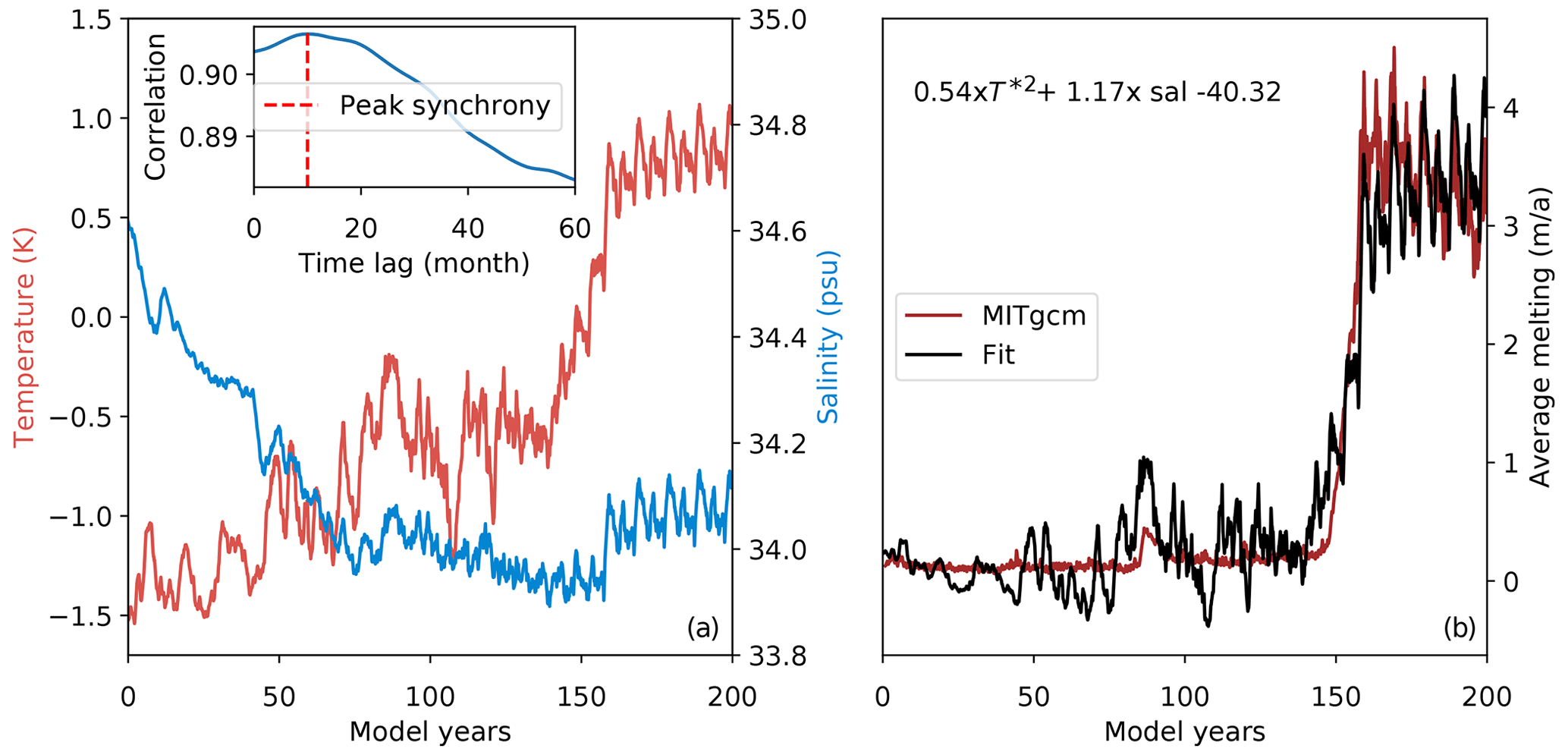
Figure A1 Filchner–Ronne Ice Shelf melt relationship estimate. (a) Evolution of average ocean temperature and salinity at the depth of the continental shelf in front of the ice shelf in the ocean simulations of the Weddell Sea in Naughten et al. (2021) for the abrupt quadrupling of CO₂. Inset shows correlation values for estimating the time lag between shelf-wide averaged melt and ocean temperatures on the continental shelf. (b) Modelled and predicted melt rates using the fitted function with parameters described in the figure.

To this aim, we relate temperatures at the depth of the continental shelf in MITgcm with melting at the ice–ocean interface. Using the average temperature over continental shelf in front of FRIS is a rough assumption that neglects complex processes that influence the in- and outflow of water masses in that cavity. However, it best reflects the assumptions and forcing used in PICO. First, we estimate the time the water masses on the continental shelf need to circulate into the cavity to drive melting using a cross-correlation. We find that a time lag of 10 months yields the highest correlation between the temperature signal and the melt signal (see inset in Fig. A1). Then, we fit a function to the modelled data of thermal driving, salinity, and melt rates using least squares. We expect the melt rates to also depend on salinity because the salinity gradient between the continental shelf and the cavity controls the strength of circulation, which in turn affects the melt rate. We assume that the (time-shifted) melt depends quadratically on thermal driving (as discussed in Sect. 2.2) and linearly on salinity. Note that we assume a linear dependency on salinity as we are not aware of a more specific functional relationship. The R² value of the fit is 0.937, and the P values for the coefficients are smaller than 0.0005, so we consider this sufficiently good. The resulting predicted melt rates show a similar pattern of increase as the modelled melt rates (see right panel of Fig. A1). Differences arise since this fit cannot capture the complicated physical processes in the Weddell Sea. This is also shown when we use the fitted relationship to predict melt in the alternative scenario from Naughten et al. (2021), which is based on a 1 % increase in CO₂ (see Fig. S7). While we can capture about an order of magnitude of melt rate increase, the fitted model amplifies the trend in melting too much and produces variability that is too large. Also in the end of the abrupt quadrupling of CO₂ (after year 160), the fitted function predicts increasing melt rates, because temperature and salinity slightly increase, while modelled melt rates slightly decrease. However, the fit is able to reproduce the large-scale pattern of the melt increase.

Naughten et al. (2021)Naughten et al. (2021)Schmidtko et al. (2014)Dutrieux et al. (2014)Jenkins et al. (2018)Schmidtko et al. (2014)

Table A1 Baseline thermal driving for FRIS and the ASE region. Values are relative to the surface freezing point.

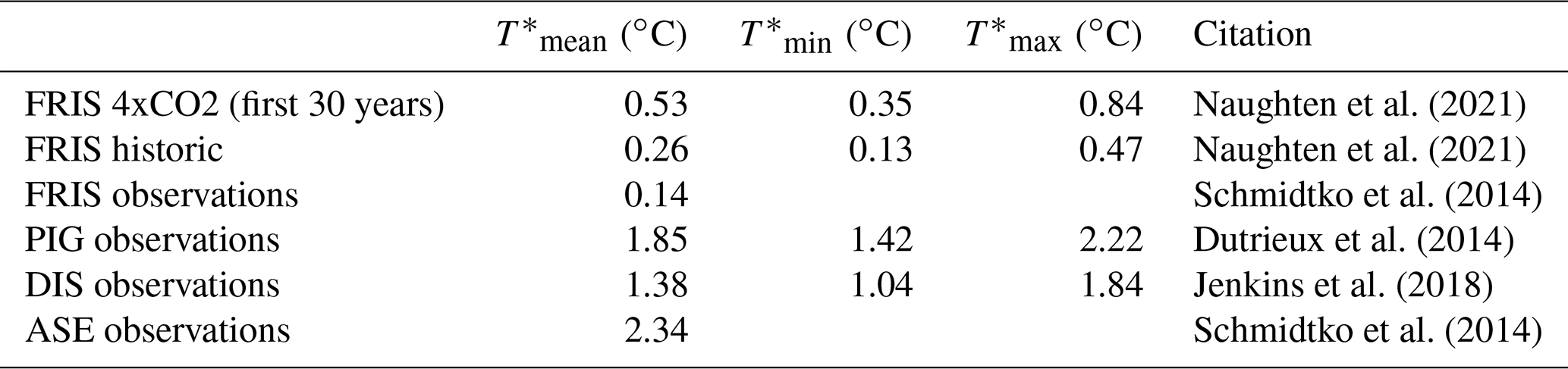
FRIS – Filchner–Ronne Ice Shelf, PIG – Pine Island Glacier ice shelf, DIS – Dotson Ice Shelf, ASE – Amundsen Sea Embayment sector.

A2 Selection of baseline temperatures

Here we describe the selection of baseline thermal driving (temperatures relative to the surface freezing point) to linearize the sensitivity between the selected thermal driving value and a warming of 1 K. The linearized sensitivity hence applies to current ocean temperatures and also captures a warming of around 1 K. While a sensitivity that is linearized around present day (±0.5 K or around 1 K below present-day temperatures) would be better suited for the historic simulations carried out in this paper, the increase from present-day levels was chosen since the numerical stability analysis of present-day grounding lines in the companion paper (Hill et al., 2023) is tested by increasing ocean temperatures above present-day levels. It also makes the sensitivity estimates suitable for projections of the Antarctic sea level contribution over the coming century. Note that if ocean temperatures change by more than 1 K, for example in simulations over longer timescales, the quadratic relationship implies that PICO, which has a linear relationship, underestimates melt rate changes.

Table A1 shows a compilation of thermal-driving values from modelling and observations. For FRIS, we list the min, mean, and max of the first 30 years of the 4xCO2 simulation with low melt rates and conditions comparable to present day, the historic simulation from 1979 to 2014, and the value from Schmidtko et al. (2014) as given in Reese et al. (2018a). For the Amundsen Sea, we use the min and max from the observations for PIG and Dotson Ice Shelf (DIS) together with the value from Schmidtko et al. (2014) as given in Reese et al. (2018a).

We use the minimum and maximum of all values for an upper and lower range of sensitivities. For the best estimate of FRIS, we use the mean of the FRIS 4xCO2 simulation, which is 0.53 ^∘C. This makes the baseline thermal driving consistent with the fitted sensitivity curve. It is warmer than the average from the data in Schmidtko et al. (2014), so it yields a slightly larger sensitivity, which is however still smaller than sensitivities estimated from other studies (see Sect. 2.2). For the best estimate in the ASE region, we use an average over available observational temperatures for DIS, PIG, and the whole region, which is 1.65 ^∘C. This value is lower than the estimate in Schmidtko et al. (2014), and hence the sensitivity is slightly lower. It is however in line with sensitivity estimates from other studies (see Sect. 2.2), and the higher value is included as the maximum sensitivity estimate.

Appendix B: PISM simulations

We show the scoring for the initial configurations in 2015 (Fig. B1) and the long-term evolution of the control simulations (Fig. B2).

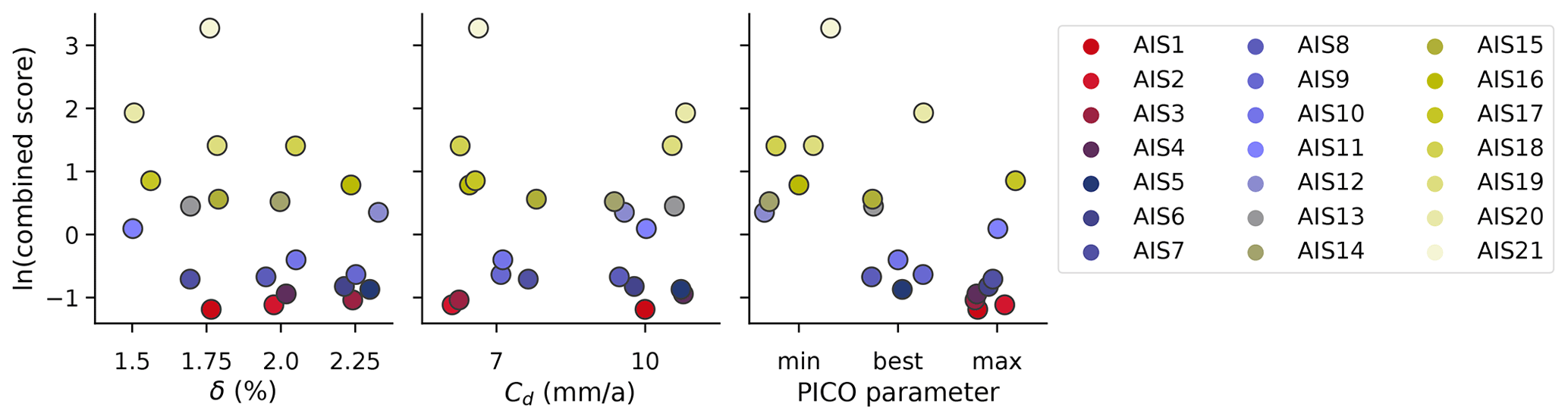
Figure B1 Scoring of ensemble of initial configurations in 2015. Scores are based on observed ice thickness, velocities, mass loss, grounding-line positions, and a special focus is given to the Amundsen, Ross and Weddell seas. Initial ensemble members were obtained from equilibrium simulations of a full parameter ensemble with all runs that showed grounding lines broadly in agreement with present-day continued after 5000 to full 25 000 years (total of 21 runs). For each a historic simulation was run from 1850 to 2015. The 2015 state is then scored with present-day observations. Shown is the natural logarithm of the scores. The lower the values the better the agreement with present day.

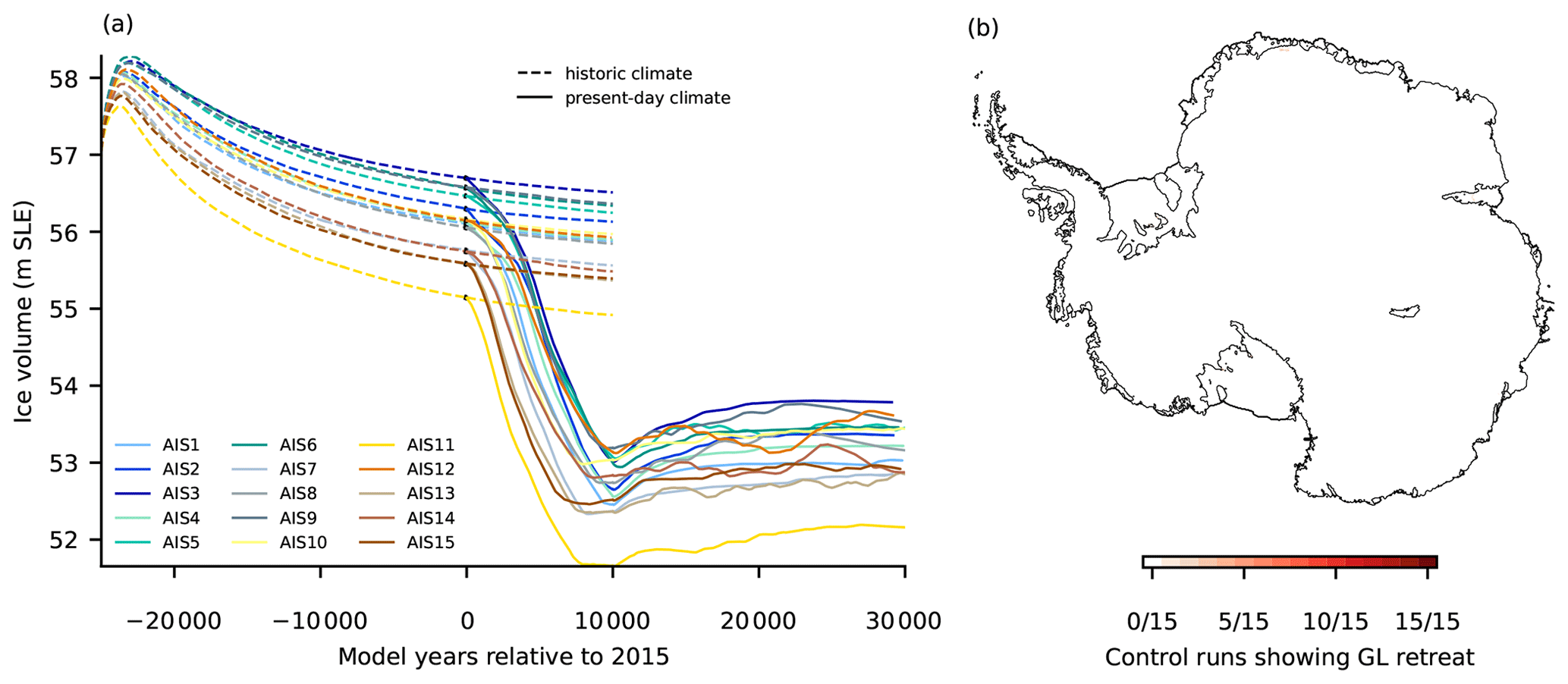
Figure B2 Sea level evolution and control runs. Panel (a) shows the evolution of Antarctic Ice Sheet volume (in metres sea level equivalent, m SLE) during the control runs and the simulations with constant present-day climate conditions and the reverse to historic conditions for all ensemble members used in the article. Black dots show historic control from 1850 to 2015. Dashed lines show control runs, solid lines show the simulations with constant present-day forcing. Panel (b) shows the regions that unground in the control runs between 1850 and year 12 015 (hardly any). The black line is the BedMachine grounding line.