the Creative Commons Attribution 4.0 License.
the Creative Commons Attribution 4.0 License.
 | 01 Sep 2023
Assimilating CryoSat-2 freeboard to improve Arctic sea ice thickness estimates
Till A. S. Rasmussen
Lars Stenseng
In this study, a new method to assimilate freeboard (FB) derived from satellite radar altimetry is presented with the goal of improving the initial state of sea ice thickness predictions in the Arctic. In order to quantify the improvement in sea ice thickness gained by assimilating FB, we compare three different model runs: one reference run (refRun), one that assimilates only sea ice concentration (SIC) (sicRun), and one that assimilates both SIC and FB (fbRun). It is shown that estimates for both SIC and FB can be improved by assimilation, but only fbRun improved the FB. The resulting sea ice thickness is evaluated by comparing sea ice draft measurements from the Beaufort Gyre Exploration Project (BGEP) and sea ice thickness measurements from 19 ice mass balance (IMB) buoys deployed during the Multidisciplinary drifting Observatory for the Study of Arctic Climate (MOSAiC) expedition. The sea ice thickness of fbRun compares better than refRun and sicRun to the longer BGEP observations more poorly to the shorter MOSAiC observations. Further, the three model runs are compared to the Alfred Wegener Institute (AWI) weekly CryoSat-2 sea ice thickness, which is based on the same FB observations as those that were assimilated in this study. It is shown that the FB and sea ice thickness from fbRun are closer to the AWI CryoSat-2 values than the ones from refRun or sicRun. Finally, comparisons of the abovementioned observations and both the fbRun sea ice thickness and the AWI weekly CryoSat-2 sea ice thickness were performed. At the BGEP locations, both fbRun and the AWI CryoSat-2 sea ice thickness perform equally. The total root-mean-square error (RMSE) at the BGEP locations equals 30 cm for both sea ice thickness products. At the MOSAiC locations, fbRun's sea ice thickness performs significantly better, with a total 11 cm lower RMSE.
- Article
(3517 KB) - Full-text XML
- BibTeX
- EndNote


With declining sea ice in the Arctic, marine traffic is increasing (Cao et al., 2022). This increases the demand for accurate sea ice predictions to ensure safety on shipping routes. Data assimilation is a commonly used tool to improve the initial state of sea ice predictions (Chen et al., 2017; Mu et al., 2018; Fiedler et al., 2022). In data assimilation, models and observations are combined using a number of approaches. For all approaches, the variables that are assimilated need to be observable and need to affect the model variable that the assimilation aims to improve. Stroeve and Notz (2015) list sea ice volume and ocean heat content as the two model variables with the largest impact on Arctic sea ice forecast. Ocean heat content is difficult to observe on an Arctic-wide scale, but sea ice concentration (SIC) and sea ice thickness can be observed from satellites (Kwok, 2010; Laxon et al., 2013; Ivanova et al., 2014; OSI SAF, 2017; Hendricks et al., 2021). While satellite-observed SIC has rather good accuracy and has been available since the late 1970s, satellite sea ice thickness observations have only been available since the early 2000s and come with large uncertainties (Laxon et al., 2003; Kwok, 2010). Several studies have found that sea ice thickness, in contrast to SIC, has a longer memory (Day et al., 2014; Stroeve and Notz, 2015; Dirkson et al., 2017). Longer memory here means that the change introduced by initial sea ice thickness persists longer than the change introduced by SIC. This makes the sea ice thickness the more suitable variable to assimilate when aiming for an improved initial estimate of the Arctic sea ice, which also has an impact on the skill of the forecast at longer timescales (Day et al., 2014).
Arctic-wide sea ice observations can only be obtained through remotely sensed data from satellites. However, for sea ice thickness, it is possible to observe the portion of the sea ice above the sea surface, which is referred to as freeboard (FB). The longest record of FB observations from a satellite with a polar orbit can be obtained from the European Space Agency (ESA) satellite CryoSat-2, which has been in orbit since 2010 (Drinkwater et al., 2004). Using an advanced radar altimeter, data from CryoSat-2 can be used to estimate FB as the difference between the observed height of the sea ice surface and the water level in leads between sea ice floes. To derive sea ice thickness from FB, a number of assumptions need to be made, which will be discussed below. These assumptions lead to a large uncertainty in the resulting sea ice thickness estimate. Therefore, we propose a method that assimilates FB directly, instead of using sea ice thickness derived from FB.
Most existing sea ice thickness products use FB measurements to calculate sea ice thickness assuming hydrostatic balance. The hydrostatic balance equation relates sea ice thickness to FB, snow density, snow thickness, sea ice density and seawater density. In this relation, FB is measured, and the other parameters are derived from climatologies or empirical values derived from in situ observations (Ricker et al., 2014; Kwok and Cunningham, 2015; Tilling et al., 2018). The abovementioned uncertainties in satellite-derived sea ice thickness largely originate from the uncertainty in these parameters (Alexandrov et al., 2010). According to Alexandrov et al. (2010), sea ice density introduces the largest error when calculating sea ice thickness from FB under the assumption of hydrostatic balance. Sea ice density depends on the ice age, where younger sea ice has a higher salinity due to more brine being enclosed in it. Over time, brine is expelled into the ocean below. During the melt season, salt is washed out by meltwater (Cox and Weeks, 1974), making multi-year ice (MYI) less saline and therefore less dense than first-year ice (FYI). Enclosed gas is another parameter that makes sea ice density estimates uncertain. FYI sea ice density uncertainty is typically around 23.0 kg m−3, and for MYI, the uncertainty is around 35.7 kg m−3 (Alexandrov et al., 2010). This high uncertainty originates from the difficulty of measuring sea ice density and the limited availability of density measurements. The density varies within the ice column depending on whether the ice is below or above sea level. On top of that, the harsh environment adds extra challenges to performing exact measurements (Timco and Frederking, 1996). Despite the variation in sea ice density, most products use fixed values of 917 kg m−3 for FYI and 882 kg m−3 for MYI (Sallila et al., 2019). The second-largest error contributor to sea ice thickness, according to Alexandrov et al. (2010), is FB. Uncertainties in FB originate from uncertainties in the sea surface height, the location of the backscattering horizon, speckle noise (Ricker et al., 2014), the retracking of the radar waveform (Landy et al., 2019), and uncertainties in snow height and density used to calculate the reduction in radar wave propagation speed in the snowpack (Mallett et al., 2020). The uncertainty introduced by the snow thickness has been extensively discussed (Kurtz and Farrell, 2011; Kwok et al., 2011; Laxon et al., 2013; Kern et al., 2015; Garnier et al., 2021). Historically, snow thickness has been derived from the Warren et al. (1999) snow climatology (W99), which was calculated from Russian drift stations for the period 1954–1991. Most of the included measurements were obtained on thick MYI. However, Kurtz and Farrell (2011) showed that W99 is less reliable over FYI compared to MYI, and Laxon et al. (2013) proposed a method to differentiate MYI and FYI snow thickness and snow density from W99. This method is now more commonly used in sea ice thickness products than the pure W99 climatology (Sallila et al., 2019). Another alternative to W99 is to use a snow model to calculate the local snow thickness, depending on precipitation. For example, Fiedler et al. (2022) showed results using snow thickness from the Forecast Ocean Assimilation Model (FOAM; Blockley et al., 2014), which is a global coupled sea ice–ocean model, or Landy et al. (2022) used SnowModel-LG (Liston et al., 2020).
W99 also includes a snow density climatology, which was commonly used in the calculation of sea ice thickness until 2020 (Sallila et al., 2019). Mallett et al. (2020) found that approximating the snow density by a linear function improves the sea ice thickness estimate by about 10 cm. Recent sea ice thickness products, for example in Hendricks et al. (2021), have started to use the proposed seasonal linear approximation of snow density, with good results. Seawater density only varies very little throughout the Arctic. Most CryoSat-2 sea ice thickness products use a single value of 1024 kg m−3, which is the density at the freezing point of Arctic surface water. The influence of the uncertainty in this value on the hydrostatic balance equation is negligible (Kurtz et al., 2013).
The uncertainties in sea ice density, freeboard (FB), snow density and seawater density all contribute to the overall error in sea ice thickness calculated from FB. To account for these errors, error estimates are used in data assimilation methods such as Kalman filters. Kalman filters rely on knowledge of the model uncertainties and observational uncertainties, as well as the assumption that they are unbiased and Gaussian distributed. Based on these assumptions, the Kalman filter aims to derive the best estimate. The accuracy of the resulting state estimate improves with better uncertainty estimates. The errors in CryoSat-2-derived sea ice thickness not only are due to the sources mentioned above, but also depend on how FYI and MYI are defined. The sea ice density; snow thickness; and, in some cases, snow density are calculated based on this ice type. The ice type is typically derived from the Ocean and Sea Ice Satellite Application Facility (OSI SAF) ice type data (Sallila et al., 2019), which distinguish between FYI, MYI and ambiguous ice types (Aaboe et al., 2021). Ye et al. (2023) assessed different sea ice type products, including the OSI SAF ice type data product, and compared them to the National Snow and Ice Data Center (NSIDC) sea ice age data (Tschudi et al., 2020). They found that the OSI SAF ice type data have for FYI a bias of 0.42×10⁶ to 0.6×10⁶ km2 and for MYI a bias of to km2. This comparison only considers FYI and MYI areas and compares them to satellite-obtained ice age products. Ambiguous areas are not considered. In most CryoSat-2 sea ice thickness products, a small transitioning area with a linear transition from MYI to FYI is assumed (Laxon et al., 2013; Tilling et al., 2018; Hendricks et al., 2021). However, the ice-chart-based sea ice type data product G10033 (Fetterer and Stewart, 2020) suggests large areas of mixed ice types. These areas are notably larger and less homogeneous than the areas suggested by the linear transition between MYI and FYI based on the OSI SAF sea ice type. This means that sea ice density, snow thickness and snow density errors are systematically underestimated or overestimated in these areas of ambiguous ice type.
As the FB error estimate is part of the sea ice thickness error estimate, it is fair to conclude that the FB error is better constrained than the sea ice thickness error. This is not to say that FB errors are unbiased. However, by choosing to assimilate FB, error contributions originating from snow thickness, snow density, sea ice density and sea ice type when converting FB to sea ice thickness are eliminated. Consequently, it follows that the FB data would be more suitable for assimilation than the derived sea ice thickness, as a lower uncertainty will increase the weight of the observed CryoSat-2 FB.
The challenge of this approach is that FB is not a sea ice model state variable but a diagnostic variable. Even though FB is not a state variable, it is related to sea ice thickness, which is a state variable and can be calculated from FB under the assumptions that a change in FB is caused only by modeled sea ice thickness and modeled snow thickness and that snow density and ice density are realistic.
In this study, we present an approach to assimilating FB directly into the sea ice model CICE (Hunke et al., 2021a). We aim to answer the following questions: does FB assimilation have a significant impact on the modeled sea ice thickness? And how does the modeled sea ice thickness after assimilation of FB compare to sea ice thickness (SIT) from a conventional CryoSat-2 sea ice thickness product? To transform FB into the model state variable sea ice thickness, we use parametrization and assumptions from the model and the forcing data. The method is implemented into CICE, but it should be applicable to any other model. This study mainly focuses on CryoSat-2 measurements, but the approach presented could also be applied to ICESat FB data (Martino et al., 2019) with small adjustments. Several studies have mentioned approaches to assimilate FB (Vernieres et al., 2016; Kaminski et al., 2018; Fiedler et al., 2022), but none has included a description of how the FB assimilation was implemented. Kaminski et al. (2018) conducted a study using the quantitative network design approach to quantify how beneficial it would be to assimilate radar FB, among other variables. The study concludes that assimilation of radar FB can improve sea ice volume simulations on the same order of magnitude as sea ice thickness assimilation. The quantitative network design approach builds upon error propagation and the sea ice thickness errors used in the analysis, which originate from the Alfred Wegener Institute (AWI) CryoSat-2 sea ice thickness products. As discussed above, this error estimate includes no contribution from ice type data and might be underestimated. To our knowledge, this is the first paper presenting detailed descriptions of an assimilation method using FB instead of sea ice thickness.
The following section presents all data sets, software and methods used to derive the sea ice thickness data sets evaluated in this study. The model setup is presented in Sect. 2.1, the assimilation setup is presented in Sect. 2.2, the observational data are presented in Sect. 2.3 and 2.4, and Sect. 2.5 presents the observation data sets which are used for validation.
2.1 Model setup
The FB assimilation is implemented in a coupled sea ice (CICE v6.2; Hunke et al., 2021a) and ocean model (NEMO v4.0; Madec et al., 2017). The coupling is based on Smith et al. (2021); however both NEMO and CICE have been updated to more recent versions. NEMO is set up following (Hordoir et al., 2022).
CICE is a multicategory sea ice model that consists of a dynamical solver, an advection scheme and a thermodynamic column physics model called Icepack. CICE and Icepack (Hunke et al., 2021b) are developed independently but are by default linked (Hunke et al., 2021b, a). The model is run with five thickness categories with category bounds that follow a World Meteorological Organization (WMO) standard setup. The upper bounds for the five categories (n) are as follows: n=1, 0.3 m; n=2, 0.7 m; n=3, 1.2 m; n=4, 2 m; and n=5, 999 m. In the presented study, CICE was implemented close to the default setup except that form drag calculations, following Tsamados et al. (2014), were enabled.
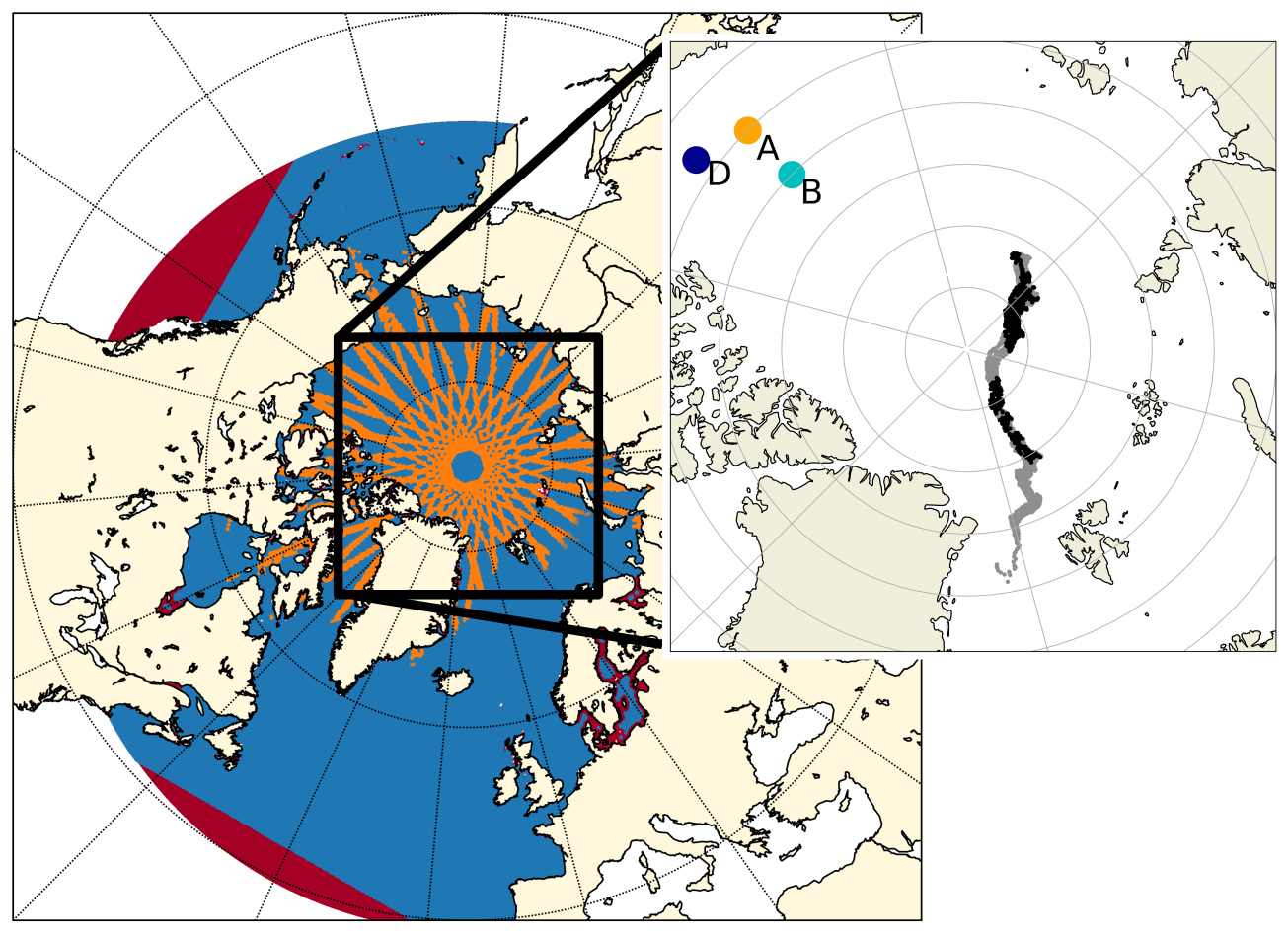
Figure 1The red area indicates the model domain (large parts are covered by the blue and orange visualization) described in Sect. 2.1, the blue area shows the OSI SAF SIC data coverage and the orange lines give example coverage of 1 week of CryoSat-2 data (here from 3 March 2020). The zoomed-in area shows the location of the three moorings described in Sect. 2.5, marked with corresponding letters, and the gray and black track indicates the drift path of the ice mass balance buoys also described in Sect. 2.5. The gray indicates the full data set used in Fig. 8 and the black the subset used in Fig. 7.
The model domain is pan-Arctic, as shown by the red area in Fig. 1 (large parts are covered by the blue and orange visualization). The lateral boundaries are located outside the Arctic sea-ice-covered region such that sea ice boundary conditions are not required. The lateral ocean boundaries are forced with monthly GLORYS12 data, which consist of salinity, temperature, and u and v velocities (Lellouche et al., 2021). The ocean model includes tides, the tidal forcing at the open boundaries originates from the TPXO 7.2 harmonic tidal constituents (Egbert and Erofeeva, 2002), and river runoff is based on a climatology from Dai and Trenberth (2002). The model is forced with 3-hourly ERA5 atmospheric forcing data, which consist of 2 m temperature, 2 m specific humidity, 10 m wind, incoming shortwave and longwave radiation, total precipitation, snowfall, and air pressure at sea level (Hersbach et al., 2017). The model runs discussed in this study are restarted from the same initial run, which runs from 1995 to 2020 and was initialized from ORAS5 (Zuo et al., 2019) ocean temperature and salinity fields. The years 2010–2020 of the initial run were used to calculate the model background error discussed in Sect. 2.2. The three other runs discussed in the following text are refRun, sicRun and fbRun: refRun consists of the initial run from 1 January 2018 to 31 December 2020; sicRun and fbRun are started from the same restart file as refRun on 1 January 2018 but assimilate (i) SIC and (ii) SIC and FB respectively. They both also cover the period 1 January 2018 to 31 December 2020. All model output discussed in the following sections is calculated based on daily means.
In order to be able to assimilate radar FB from CryoSat-2, a new variable for radar FB needs to be introduced in CICE. For this we combined Eq. (4) from Alexandrov et al. (2010) with Eq. (12) from Tilling et al. (2018) as follows:
Here, hi is the modeled sea ice thickness from CICE, ρw is the modeled surface water density from NEMO, hs is the modeled snow thickness from CICE, c is the speed of light in vacuum (3×10⁸ m s−1) and cs the speed of light in snow. The variable cs is calculated following Eq. (2):
Mallett et al. (2020) compared constant ρs values to the seasonal linear variation in ρs derived by Warren et al. (1999) and concluded that a seasonally varying ρs can improve FB-derived sea ice thickness estimates by up to 10 cm. The original value used in CICE is constant and equals 330 kg m−3. In this study it was substituted with the derived relation from Mallett et al. (2020) following Eq. (3):
where t is time counted in months since October. The relation in Eq. (3) is only used in the radar FB calculation for the assimilation and nowhere else in the sea ice model. CICE uses constant ρi values, but for the radar FB calculation, a variable sea ice density was needed, since ρi has significant impact on Eq. (1) (Alexandrov et al., 2010; Kern et al., 2015). Sea ice density is dependent on the air bubbles enclosed in the sea ice and on the brine content (Timco and Frederking, 1996). Brine content in sea ice results from the brine rejection during freeze-up and drains over time. If the brine channels are not filled with water, they remain as air bubbles in the ice (Timco and Frederking, 1996). CICE calculates the salinity content in sea ice and the density of sea ice without accounting for a changing number of air pockets. To calculate the sea ice density, we divide the sea ice volume in one grid cell into fresh ice and brine, calculate the percentage of the fresh ice and brine, and weight a fresh ice density (ρi0) and the brine density (ρb) with this.
Here, aiceb is the amount of brine as a percentage of the total ice volume. The variable ρi0 was set to 882 kg m−3 following Alexandrov et al. (2010) values for MYI sea ice density. In the following text, FB stands for the radar FB.
2.2 Assimilation setup
Kalman-filter-based assimilation is a widely used technique that employs an ensemble of model forecasts to estimate the state of a system using available observations. The method involves three main steps: a forecasting step, a filtering step and a re-sampling step. The forecast is performed by the model. During the filtering step, the ensemble members are adjusted based on knowledge of the model background error, observation error, model states and observations to obtain the best possible estimate of the system state. In the re-sampling step, the best estimate from the filtering step is used to update the ensemble members. This process is repeated iteratively in order to improve the accuracy of the state estimate. For the filtering step, we use the Local Error Subspace Transform Kalman Filter (LESTKF) (Nerger et al., 2012), which is included in the Parallel Data Assimilation Framework (PDAF) (Nerger and Hiller, 2013). LESTKF has, prior to this study, successfully been used to assimilate SIC and sea ice thickness, for example by Chen et al. (2017). In this study, PDAF is used offline, which means that the assimilation scheme runs independently of the ocean and sea ice model. The consequence is that the ocean and sea ice model needs to be restarted when the model and the assimilation exchange information. PDAF was run separately for SIC and FB. Figure 2 illustrates the data flow between the different components. The numbers noted in the lower corner of each component correspond to each of the following sections, describing which part of the assimilation is handled in which program.
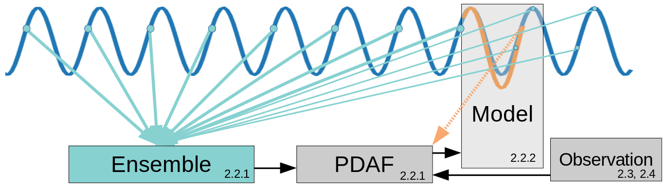
Figure 2General setup of the assimilation routine. The dark-blue curve indicates the initial model run and the orange curve the assimilated run, with the dashed orange arrow indicating the model state at the assimilation time. The thick turquoise arrows indicate the 8 d chosen around the assimilation date and the thin turquoise arrows the 4 (or 3) d chosen ± 2 months around the assimilation date (described in Sect. 2.2.1). The numbers in the lower corners indicate in which section of the paper the different elements are described.
2.2.1 PDAF
PDAF inputs consist of the model state, model ensemble, observations and observation uncertainties in the model grid. The spread of the ensemble is used to calculate the model background error used in the filtering step. In this study, we only run one model realization and calculate the model background error in the Kalman filter from a static ensemble, similarly to the setups in BAL MFC (Nord et al., 2021) and SAM2 (Tranchant et al., 2006). Using a static ensemble has the advantage of lower computational cost. To calculate the model background error based on a static ensemble, a free model run of the model used in the assimilation is needed. In our case the free model ran from 1995 to 2020, but only the years 2010–2020 were used to construct the static ensemble as the earlier years were considered spinup. The justification of using a static ensemble is based on the assumption that the model error on a certain day in a year is reflected by the interannual model variability of this same day. Knowing the biases of the model allows for the correction of this assumption. In our case, the model overestimates the ice extent, which we found when comparing the 10-year initial run to OSI SAF (Saldo, 2022) SIC observations. Thus, the background error based on the same date in several years would not result in a large enough spread to weight the observations correctly. The ensemble used to calculate the model background error consists of 80 members, and it is constructed as follows: each of the 10 years from the free run contributes 8 d.
-
In 8 years, a period of 8 consecutive days is chosen, starting from the date 3 d prior the assimilation time step and ending 4 d past it.
-
In 2 years, a period of 3 consecutive days from the date 2 months prior to the assimilation time and a period of 4 consecutive days from 2 months past the assimilation time are chosen.
After the ensemble members were chosen, they are averaged. This average is then subtracted from each member, and the resulting variation is added to the model state at the assimilation date. These 80 ensemble members are then used to calculate the model error. For the observation error, we use the error estimates provided in the data sets.
2.2.2 Integration of increments
The physical model in Sect. 2.1 utilizes the Kalman filter increment, which is the correction that adjusts the model state to the optimal state based on observations and model states. This increment is obtained as the difference between the model state input to PDAF and the analyzed state. The model state is corrected towards the analyzed state by subtracting the increment from the model state. To ensure stability, the increment is divided by the number of time steps (number of model time steps in one assimilation time step), which results in the fractal increment or the amount of change needed per model time step (following Eq. 5). This fractal increment is hereafter subtracted at each time step from the model value. This method is called incremental analysis updating and was introduced by Bloom et al. (1996). For SIC, this method is straightforward, since the observations are also what we aim to assimilate.
FB needs to be converted into sea ice thickness, and if this were to be done separately at each time step, the changing sea ice density and snow thickness could potentially influence the resulting sea ice thickness. Similarly to SIC, the FB increment is subtracted from the model state at t0. To convert FB to sea ice thickness, Eq. (1) was rewritten as follows:
The variable newice is now subtracted from the modeled sea ice thickness and linearly spread following Eq. (5).
At each time step, we have the fractional increment of SIC and sea ice thickness to be subtracted from the model state. The model used in this study is a multicategory model. Therefore, the grid cell average increment must be spread over the five model categories. To achieve this, Eq. (7) was used. Here varold is the SIC at the current time step, varold(n) is the SIC in n categories, inc is the SIC increment and n is the thickness category.
In the case where SIC and FB are negative after the assimilation, they are rounded to 0. In cases where the SIC ends up above 1, SIC is rounded to 1. FB is only assimilated if SIC is above 80 % and if sea ice thickness is above 0.05 m. These thresholds were chosen not only for stability, but also because thin FB is not measured accurately (Wingham et al., 2006; Ricker et al., 2014) and because FB is calculated from the model's ice volume per unit area of ice. In areas with lower concentrations, this can lead to SIT and FB values that are unrealistically high. To avoid overestimation of FB following this artifact, a high SIC threshold was chosen for the FB assimilation.
2.3 CryoSat-2 radar altimetry freeboard and sea ice thickness
The observed FB assimilated in this study is level-3 weekly gridded CryoSat-2 radar FB downloaded from the Alfred Wegener Institute (AWI) sea ice portal (version 2.4; Hendricks et al., 2021). This comprises gridded, along-track data on the EASE2-Grid with a 25 km resolution. The radar FB is defined as the elevation of a retracked point above instantaneous sea surface height without snow range correction. The data product is derived from the CryoSat-2 Baseline-E data, the mean sea surface model DTU21 and the threshold first-maximum retracker algorithm (TFMRA) (Ricker et al., 2014).
With the onset of melt at the beginning of summer, melt ponds are formed on the sea ice surface. The radar signature from melt ponds is comparable to the signature from leads, which can result in ambiguous determination of the sea surface height. This ambiguity results in a larger bias in the FB measurements, and FB data are therefore only assimilated from November to March, when we do not expect melt ponds. The uncertainty in FB given in the AWI data set ranges on average from 0 to 0.07 m in the chosen month. The data set was bi-linearly interpolated to the model grid with help of Climate Data Operators (CDO; Schulzweida, 2022). An example of the FB data assimilated per assimilation time step (1 week) is indicated by the orange lines in Fig. 1.
The data set also contains sea ice thickness derived by assuming hydrostatic balance, which is the method referred to as the classical approach. In order to obtain sea ice thickness from FB, hydrostatic balance is assumed, and sea ice thickness is calculated as described in Eq. (6). In the AWI CryoSat-2 data set, the snow thickness from Warren et al. (1999) snow climatology was applied over MYI, and NSIDC AMSR2 snow depth (Hendricks et al., 2021) was applied over FYI. The snow density is calculated following Eq. (3) from Mallett et al. (2020), and the sea ice density is set to 916.7 kg m−3 for FYI and to 882.0 kg m−3 for MYI. MYI and FYI are distinguished with the help of OSI SAF ice type data. For a more detailed description of the data set, see Hendricks et al. (2021).
2.4 OSI SAF data
Ocean and Sea Ice Satellite Application Facility (OSI SAF) SIC is assimilated in this study. It is based on passive microwave measurements of the Special Sensor Microwave Imager/Sounder (SSMIS), which is onboard a polar-orbiting satellite. The OSI SAF algorithm combines SSMIS microwave measurements with numerical weather prediction (NWP) model output from ECMWF in order to calculate SIC. Passive microwave measurements are independent of visible light, which makes this sensor type especially suitable in polar regions. The data set used is the climate data record (CDR) OSI-430-a, which is gridded on a 25×25 km grid once a day. The data can be downloaded from the Norwegian Meteorological Institute FTP servers: ftp://osisaf.met.no/reprocessed/ice/conc/v3p0 (last access: 12 January 2023). The presented data set was chosen after examining the error estimates in the different data products. The comparison showed that the CDR is the only data set that has no large error fluctuations over open-water areas. More details on the error estimate can be found in Saldo (2022). Studies have found that the summer melt ponds lead to underestimated SIC in satellite passive microwave measurements (Kern et al., 2016; Ivanova et al., 2013; Rösel and Kaleschke, 2012). This is the reason we decided to only assimilate SIC during the months November to March.
For the assimilation, the data set was bi-linearly interpolated onto the model grid using CDO (Schulzweida, 2022). The resulting SIC data coverage assimilated is indicated by the blue area in Fig. 1.
2.5 Validation data
Two in situ sea ice observation data sets are used for validation. The Beaufort Gyre Exploration Project (BGEP) upward-looking sonar (ULS) sea ice draft data set and 19 ice mass balance (IMB) buoys deployed during the Multidisciplinary drifting Observatory for the Study of Arctic Climate (MOSAiC) campaign measuring sea ice thickness. The advantage of these observations is that they are independent of the assimilated data; however each observation has limitations in terms of time and space.
The BGEP ULS sea ice draft data set can be downloaded from https://www2.whoi.edu/site/beaufortgyre/data/mooring-data/ (last access: 28 June 2023). The ULS data are obtained from three locations named moorings A, B and D, marked with orange, turquoise and dark-blue dots in Fig. 1. The data cover 2 years, from October 2018 to November 2020. The instruments are located 50–85 m below the water surface and measure the ice draft with a frequency of 2 s over a 2×2 m area. The signal is filtered and averaged over 10 s intervals in order to correct for tilting errors. Tilting error refers to the error that results from the movement of the ULS when ocean currents move the instrument and so influence the distance to the sea ice. The error is assumed to be random; hence averaging the data will eliminate it. The sea ice draft accuracy is ±5 cm.
For the comparison of BGEP observations and model and AWI data, the model and AWI draft was calculated as sea ice thickness minus sea ice FB. To compare the BGEP data with the three model runs, the daily average and standard deviation (SD) were calculated from the differences of all 10 s measurements and the model daily output. For the comparison, only the grid cell which would cover the respective buoy was considered. Since the resulting daily mean and SD were still too variable, they were further smoothened by a 7 d running mean. For the comparison of the fbRun, AWI and BGEP draft, only weeks in which the AWI data cover the BGEP locations were considered. The model values are weekly means of the respective buoy covering the grid cell.
To be able to compare sea ice in situ measurements from more locations, the IMB buoy deployed during the MOSAiC campaign are used (Lei et al., 2021). In contrast to the stationary measurements from the BGEP, the measurements drift along the black trajectory in Fig. 1, from the center of the Arctic towards Greenland. The IMB buoy includes a thermistor string reaching from the snowpack top to the ice–ocean interface at the bottom. A thermometer and a heating element are located each 2 cm. The ice–snow, ice–water and snow–air interfaces are measured by heating the thermistor string up and measuring the thermal response. More information on the instrument can be found in Jackson et al. (2013). The IMB buoys measure the thickness of only one ice flow, unlike the BGEP upward-looking sonar, and the data have a temporal frequency of one measurement per day. To ensure that the comparison between the buoys and the gridded AWI sea ice thickness and model output is reliable, 19 IMB buoys were considered. However, not all buoys were active at the same time. All buoys were interpolated to the model grid by the nearest-neighbor method.
For a comparison of the different model runs vs. the IMB measurements, a minimum of eight active buoys per day were chosen. The limit of eight buoys was chosen to account for the spatial coverage of the active buoys and at the same time secure a sufficient number of days in which at least eight buoys were active.
For the IMB sea ice thickness vs. assimilated sea ice thickness and the AWI sea ice thickness comparison, the IMB buoy coverage of 1 week was projected onto the model grid, choosing the nearest neighbor. For the model data, only grid points covered by the AWI data and the IMB buoys were chosen, and weekly averages were calculated for all three products. No threshold of a minimum number of active buoys was chosen, as this would have limited the available data too much.
3.1 Freeboard and sea ice concentration RMSE
To verify that the assimilation improves the modeled FB and SIC, the root-mean-square errors (RMSEs) between the assimilated data sets and the model variables were computed after each assimilation time step. The calculation of RMSE includes all observed data points of the assimilation time step. RMSE for FB is calculated on the available satellite tracks (marked orange in Fig. 1), which change every week, and the co-located model values. The same approach is used for SIC (the blue area in Fig. 1) and the corresponding model data.
The results are shown in the upper panels of Figs. 3 and 4, and they are based on mean weekly model output data at the location where the corresponding observations exist. The lower panels in both figures show the difference between refRun and sicRun or fbRun. Positive values indicate that the assimilation has improved the SIC or FB, and negative values indicate that the variable was degraded by the assimilation. Degradation can occur when an assimilation variable disturbs the physical balance of the model and during a period of free run, when it is in the process of reestablishing its physical balance.
The results (Fig. 3, upper panel) show that the reference run (black) had the highest RMSE of all and that the RMSE increased the most over the assimilation period. This indicates that the assimilation improved the modeled sea ice concentration. The RMSE for the assimilated runs (sicRun in turquoise and fbRun in orange) also increased over the assimilation period but to a lesser extent than for the reference run. The lower panel in Fig. 3 shows a steady increase in the difference between the reference run and the assimilated runs, reflecting the degree to which assimilation improved sea ice concentration.
The increase in RMSE over the season is a result of the chosen area for calculating RMSE and the definition of the metric itself. RMSE weights larger errors more heavily than smaller errors. The FB differences are only calculated over areas with sea ice, while the SIC data include larger areas that are seasonally either ice-free or ice-covered. For SIC, the area with the largest error, which is weighted most, is the ice edge at the Atlantic side, which increases over winter, accounting for the observed seasonal increase in SIC RMSE from November to March in Fig. 3. Other assimilation studies have chosen to calculate RMSE only over ice areas with sea ice concentration above 15 % (Chen et al., 2017), but to be consistent, we chose to calculate RMSE over the entire area.
The lower panel in Fig. 3 also shows negative values in October for the last 2 years, indicating that the assimilated runs agree less with the assimilated data compared to the reference run at the beginning of the assimilation period. The RMSE difference in the lower panel falls below 0 at the beginning of all assimilation periods after the initial one. As noted earlier, this can occur if the physical balance of the model is disturbed by assimilation.
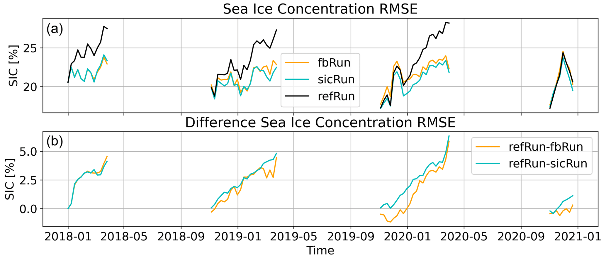
Figure 3(a) Weekly SIC RMSE calculated at the observation data location, averaged over the corresponding assimilation time step. The orange plot shows the fbRun RMSE, the black the refRun RMSE and the turquoise the sicRun RMSE. (b) The differences in the top-panel RMSEs of refRun − fbRun in orange and refRun − sicRun in turquoise. The date format is year-month.
The upper panel of Fig. 4 displays the RMSE of all FB values assimilated at the corresponding time. The black line represents refRun, while the turquoise line represents sicRun. Both have almost equal FB RMSE throughout the assimilation period, ranging between 7 and 14 cm. The black refRun covers the turquoise sicRun in the upper panel. On the other hand, the FB RMSE for fbRun shows a clear drop within the first month of the assimilation period, reducing to about 5 to 6 cm. The lower panel in Fig. 4 shows that the RMSE differences are all above 0, even at the beginning of a new assimilation period in November.
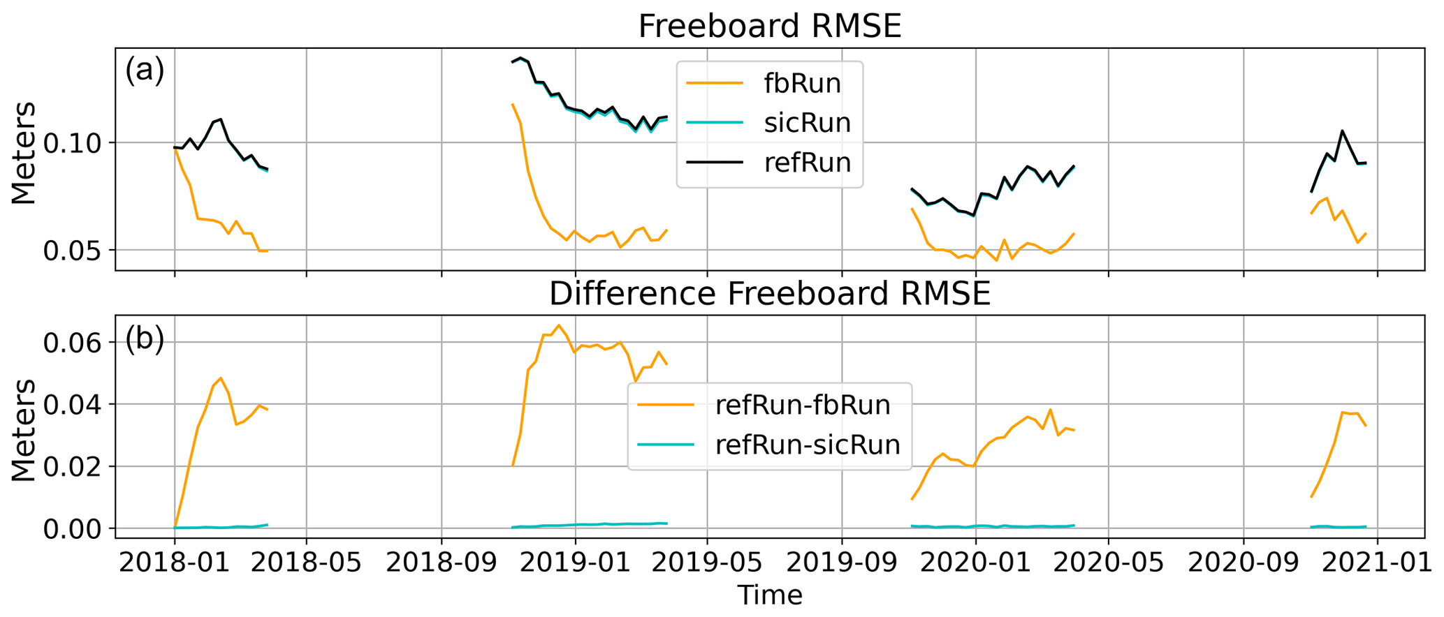
Figure 4(a) Weekly FB RMSE calculated at the observation data location, averaged over the corresponding assimilation time step. The orange plot shows the fbRun RMSE, the black the refRun RMSE and the turquoise the sicRun RMSE. The black plot indicating refRun covers the turquoise plot indicating sicRun most of the time. (b) The differences in the top-panel RMSEs of refRun − fbRun in orange and refRun − sicRun in turquoise. The date format is year-month.
It is expected that the SIC RMSE in Fig. 3 and the FB RMSE in Fig. 4 show improvements, as the observation values are used within the assimilation scheme; however this demonstrates that the assimilation works.
3.2 CryoSat-2 AWI sea ice thickness
To demonstrate that the sea ice thickness estimated through the FB assimilation method provides comparable results to other sea ice thickness products derived from CryoSat-2, the sea ice thickness of fbRun was compared to the AWI sea ice thickness. The AWI sea ice thickness was selected because it is derived from the same FB values as the FB data assimilated in fbRun. Any differences between the two data sets therefore indicate the impact of the FB assimilation introduced here in contrast to the method of directly converting FB to sea ice thickness.
Table 1Monthly mean correlation coefficient and mean bias between the weekly AWI sea ice thickness (SIT) and FB and the fbRun SIT and FB for the entire assimilation period from 1 January 2018 to 31 December 2020. Only grid points covered by both the AWI FB data and the model were considered.

Table 1 presents the correlation coefficients and biases for sea ice thickness and FB in refRun and fbRun compared to the AWI data. All spatially coinciding data points of the model runs and the AWI data were considered over the entire period from 1 January 2018 to 31 December 2020. In general, the lowest correlations and highest biases are found in October, as no data had been assimilated yet and the assimilation period started in November.
The sea ice thickness biases are negative for all months and runs, indicating that the modeled sea ice thickness and FB are thinner than the AWI data's FB and sea ice thickness. The sea ice thickness biases for both runs are smallest in January, and the FB biases are smallest in January and February. Overall, the FB biases are thinner than the SIT biases, which is no surprise as FB is typically on the order of about 10 % of sea ice thickness (Alexandrov et al., 2010).
Comparing the correlation coefficients of refRun and fbRun for both the FB and the sea ice thickness shows that the difference between the FB correlation coefficients is higher than the difference between the sea ice thickness correlation coefficients. This indicates that the FB assimilation brings the modeled FB closer to the assimilated FB data but that the difference in deriving the SIT from the FB data also impacts the resulting SIT.
Figure 5 displays bivariate and univariate kernel density estimates (KDEs) for sea ice thickness (panels a and b) and FB (panels c and d) for fbRun (in orange) and refRun (in blue) compared to the AWI data. The months of October and December were displayed as they represent the lowest and highest sea ice thickness correlation (see Table 1).
The KDE for both variables of fbRun changes from October to December, indicating higher correlation coefficients and smaller biases in December, which is a result both of thin and thick sea ice and of FB getting thicker. However, the thicker FB and sea ice thickness values are still thinner than the AWI data variables, while the thin FB and sea ice thickness values are thicker than the AWI values. This could be a result of the assimilation discarding negative FB values in the model, while the AWI data set includes negative FB values.
For the month following December (not displayed), the center of the sea ice thickness KDE (at about 1 m in Fig. 5b) falls, month by month, further below the black regression line, while the thick sea ice thickness compared to refRun shows similar improvements to the December plot. This indicates that the decreasing correlation and increasing bias (Table 1) originate from fbRun’s sea ice thickness and FB becoming thinner compared to the AWI data sets values, while the thick sea ice compares equally well to the AWI sea ice thickness.
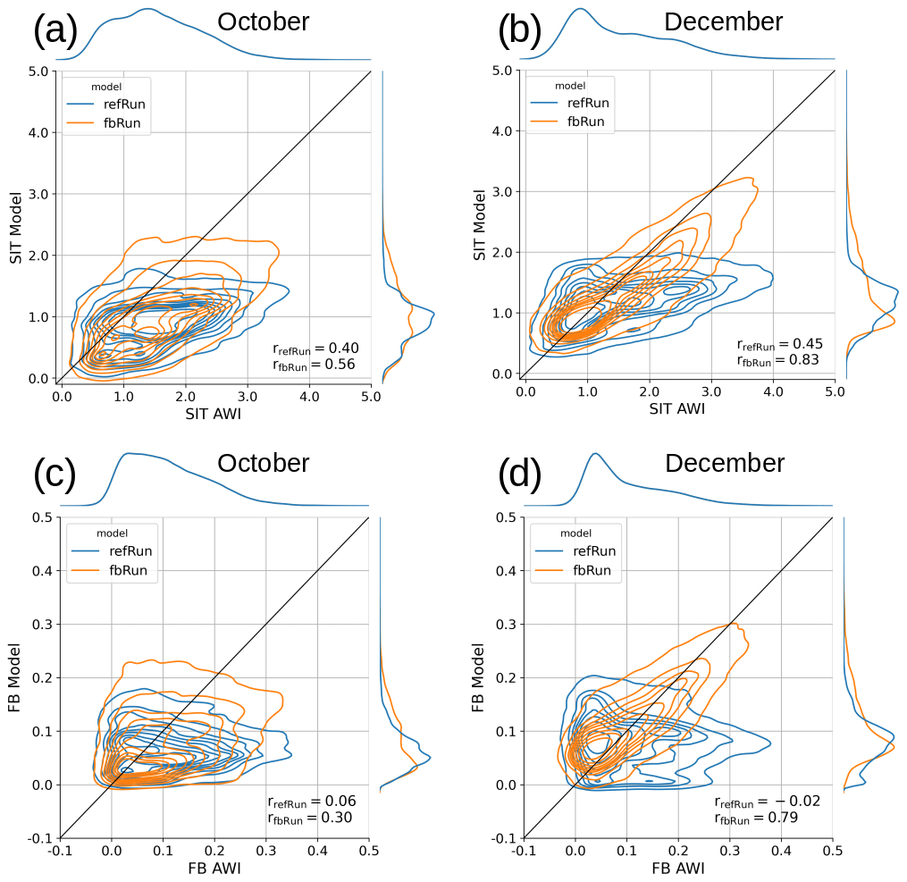
Figure 5The bivariate and univariate kernel density estimate (KDE) for sea ice thickness and FB for the model runs fbRun and refRun in comparison to the AWI sea ice thickness and FB. Panels (a) and (b) show the sea ice thickness in October and December, and panels (c) and (d) show the FB for October and December. The months October and December were chosen because October is the month with the lowest sea ice thickness correlation between fbRun and AWI (as listed in Table 1). The correlation coefficients r are displayed in the lower-right corner of each plot. The black line indicates r=1, and the unit is meters.
3.3 Upward-looking sonar data
The BGEP upward-looking sonar sea ice draft is independent of the satellite-derived FB data, and it is used for the comparison of the modeled sea ice draft, which is calculated as described in Sect. 2.5. The BGEP data are not available for the complete period from 1 January 2018 to 31 December 2020; hence only data from October 2018 to December 2020 are used.
The BGEP ULS data, model data and AWI sea ice draft data are provided at different spatial and temporal coverage levels. To compare the different data sets, we split the comparison into two parts in order to account for these differences. In Fig. 6 the model drafts from all three model runs are compared to the BGEP ULS drafts based on mean daily differences, whereas, Fig. 7 compares the AWI draft and the fbRun draft with the BGEP ULS drafts based on mean weekly differences only at locations covered by the AWI data. The differences between the BGEP upward-looking sonar ice draft and the model sea ice draft are shown in Fig. 6. The dashed line shows fbRun, the solid line refRun and the solid line with circle markers sicRun. The gray-shaded areas indicate the assimilation period.
Table 2RMSE calculated between the BGEP ULS draft measurement and the model runs fbRun, sicRun and refRun and the MOSAiC IMB sea ice thickness and the model runs. The RMSE and biases were calculated for all three mooring locations together, the assimilation period marked gray in Fig. 6 and the free-run period.
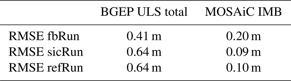
For all three moorings, fbRun shows the values in closest agreement with the observations throughout the entire period displayed. This is also reflected by the lower RMSE listed in Table 2. The runs refRun and the sicRun are almost in perfect agreement except for on a few days, for example in October 2019 at BGEP moorings A and D. The RMSE between the BGEP data and fbRun is with 0.41 m, 23 cm lower than the RMSE of refRun and sicRun. Periods in summer, when the observation SD is 0 m, indicate periods with no ice present in the observations. Gaps indicate periods where no data are available. The BGEP observations are all ice-free in summer 2019, while only fbRun at BGEP mooring A reaches the point of being ice-free in late September continuing until the beginning of November 2019.
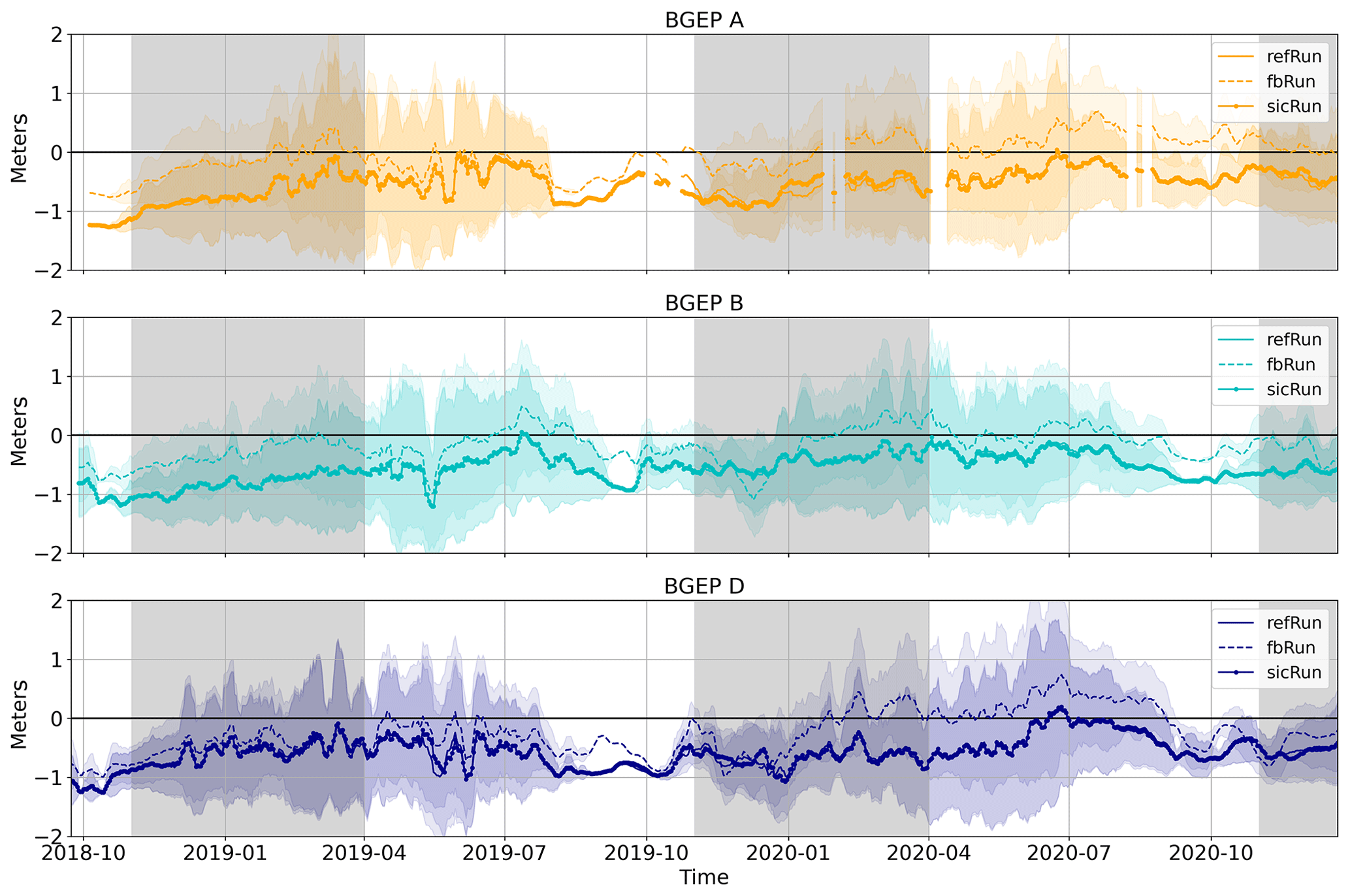
Figure 6Daily mean sea ice draft differences and SD between BGEP observations and all three model runs. The shaded colored area shows 1 SD calculated for each day from the 10 s record. The SD appears darker where the SDs from different model runs overlap. The gray-shaded area indicates the assimilation period. The dashed line shows observed sea ice draft minus fbRun sea ice draft, the solid line the equivalent for refRun and the solid line with circle markers the equivalent for sicRun only. Panel (a) shows data from mooring A, panel (b) data from mooring B and panel (c) data from mooring D. The sites are marked in the corresponding colors in Fig. 1. The date format is year-month.
Figure 7 shows the mean differences between the AWI sea ice draft and the fbRun sea ice draft. To do so, the AWI data set was interpolated to the model grid and only data points covered by all three data sets (AWI CryoSat-2, fbRun and BGEP) were considered. Instead of daily averages as shown in Fig. 6, weekly averages were calculated, since the AWI sea ice draft is provided in weekly time steps. The dashed lines in Fig. 7 show the AWI data and the solid lines the fbRun data. The gray background shows the assimilation period. Colors are chosen per mooring according to Fig. 1. The resulting differences between the fbRun and the AWI CryoSat-2 sea ice draft are shown in Fig. 7. Both the AWI sea ice draft and the fbRun sea ice draft differ by about ±50 to 90 cm from the mooring data. There is no clear bias or seasonality in either difference, and they do not always follow the same pattern, except in winter 2019/20, when both data sets begin with a negative bias and end with a positive bias with the exception of a few weeks in the AWI CryoSat-2 draft at the end of the assimilation period.
Table 3The mean RMSE of the weekly mean differences shown in Fig. 7. The RMSE was calculated on average for each mooring and both the fbRun ice draft and the AWI CryoSat-2 ice draft.
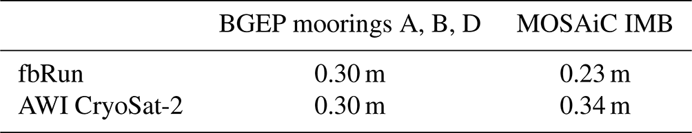
The RMSEs between the BGEP moorings' sea ice draft, the fbRun sea ice draft and AWI CryoSat-2 sea ice draft were calculated. They are listed in Table 3. The RMSEs of the data products compared to the mooring data are both 0.3 m.
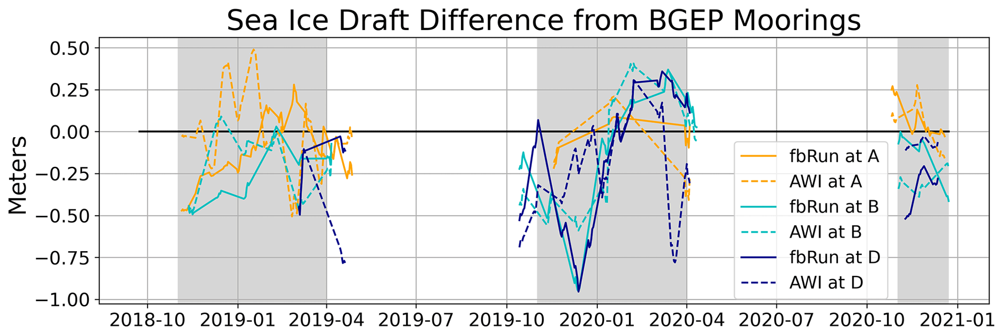
Figure 7The weekly mean difference between the BGEP upward-looking sonar sea ice draft measurements and sea ice draft calculated from the AWI sea ice data set (dashed lines) and the fbRun sea ice data (solid lines). The color indicates the location in Fig. 1. Positive values indicate that the BGEP draft is thicker. The date format is year-month.
3.4 MOSAiC IMB data
The MOSAiC data cover a different spatial area than the BGEP observations. Data are interpolated to daily and weekly means respectively in order to have the same frequency as the data that they are being compared to. Details are described in Sect. 2.5.
In Fig. 8, the daily sea ice thicknesses from the MOSAiC IMB buoys and the three model runs are plotted for days when at least eight buoys were active. The shaded area around each line indicates 1 SD of the respective displayed data. The MOSAiC IMB data set has the largest SD, and all model runs lies within this SD for most of the observation period, with the exception of fbRun's sea ice thickness in October 2019, April 2020 and June 2020. Overall, the modeled, assimilated and observed sea ice thicknesses grow over the same period from October 2019 to April 2020, and all four sea ice thicknesses also start to decline at about the same time in June 2020. The observed sea ice thickness starts to be more variable at the beginning of June 2020, which is not reflected in the model data. The variability in the observation data is most likely caused by the reduced number of buoys that are active during this time and the sea ice being more mobile as it starts to melt. Both the refRun and the sicRun sea ice thicknesses compare better than fbRun to the MOSAiC observation. This is also reflected in the RMSE calculated for fbRun, sicRun and refRun in comparison to the MOSAiC sea ice thickness in Table 3. A one-sided t test was performed, comparing the differences between the different model runs and the MOSAiC IMB sea ice thickness. The one-sided t test showed that sicRun's and refRun's sea ice thickness RMSE was significantly lower than fbRun's RMSE.
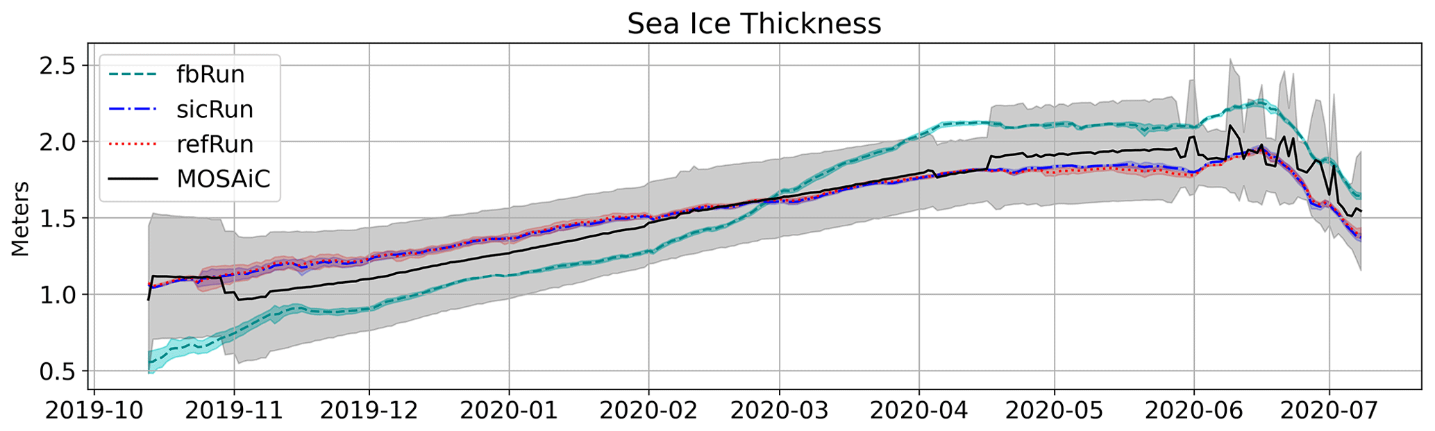
Figure 8Daily mean sea ice thickness averaged over all grid cells covered by at least eight active buoys per day. The solid black line indicates the MOSAiC IMB-buoy-measured sea ice thickness, the dotted red line the refRun sea ice thickness, the dash-dotted blue line the sicRun sea ice thickness and the dashed turquoise line the fbRun sea ice thickness. The shaded areas around each of the plots indicate 1 SD of each daily averaged sea ice thickness data set. The date format is year-month.
Figure 9 shows the weekly mean sea ice thickness from the MOSAiC IMB buoys and the three model runs. The average is calculated as described in Sect. 2.5. The dash-dotted yellow line represents the AWI sea ice thickness, the dashed turquoise line represents the fbRun sea ice thickness and the solid black line represents the MOSAiC sea ice thickness. The transparent shaded background in each corresponding color indicates 1 SD. All three sea ice thicknesses increase over the displayed period. The AWI sea ice thickness increases the most from approximately 0.6 to 2.3 m with a sharp drop in the last week of April. The MOSAiC data display less growth and start slightly thicker than both the fbRun and AWI sea ice thickness at around 0.8 m in October 2019 and reach around 1.8 m in April 2020.
When comparing the sea ice thickness for fbRun from Figs. 8 and 9a, it is apparent that the fbRun sea ice thickness follows a similar pattern. However, this is not the case for the MOSAiC sea ice thickness. Comparing the sea ice thickness for the MOSAiC IMB data from Figs. 8 and 9a, the data in Fig. 9a appear to be more abundant. This difference is caused by the number of buoys considered. The buoys considered in Fig. 9 depend on the sparse AWI data coverage, while Fig. 8 considers at least eight buoys per day. This leads to larger jumps from week to week of the MOSAiC sea ice thickness in Fig. 9 compared to Fig. 8. This is also evident by the low SD at the beginning of March and in mid-April 2020 in Fig. 9.
Table 3 lists the RMSE calculated between the AWI and the MOSAiC sea ice thickness and between fbRun and MOSAiC sea ice thickness. The RMSE calculated for the AWI sea ice thickness is 11 cm greater than the RMSE calculated for the fbRun sea ice thickness. A one-sided t test was performed to determine the statistical significance of the difference, which showed that the fbRun RMSE is significantly smaller than the AWI RMSE.
In Fig. 9b, the radar FB for the refRun, fbRun and AWI data are shown. The fbRun and AWI data FB in Fig. 9a and the respective sea ice thicknesses in Fig. 9b do not entirely follow the same pattern. The AWI FB starts out thinner than fbRun's FB, while the AWI sea ice thickness is thicker than fbRun's sea ice thickness throughout the entire displayed period. This indicates that the difference is caused by the difference in snow thickness and sea ice density. The AWI data are the FB values that were assimilated, and the fbRun FB is approximately between refRun's and AWI data values, showing the effect of the assimilation. It is clear from Fig. 8 that refRun and sicRun are closer to MOSAiC IMB data; however Fig. 9 shows that the fbRun follows the evolution of the observed radar FB better. This shows that the assimilation acts as expected, but in this area there is a discrepancy between the in situ observations from MOSAiC IMB buoys and the remotely sensed AWI FB observations. The relation between the FB from refRun and fbRun follows a similar pattern to the sea ice thickness in Fig. 8, since the sea ice density, snowfall and water density values are not significantly influenced by the assimilation.
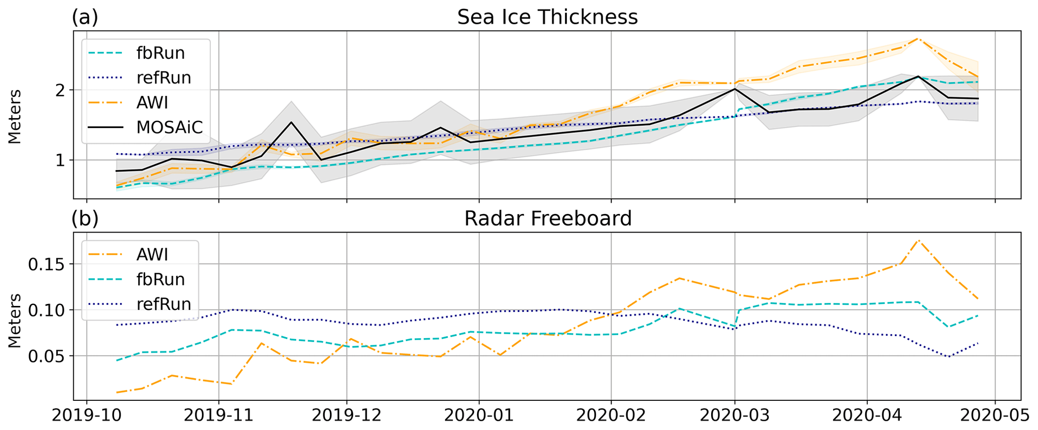
Figure 9(a) Weekly mean sea ice thickness averaged over all grid cells covered by the CryoSat-2 flight pass considered in the AWI data set. The mean sea ice thickness is displayed with 1 SD for sea ice thickness from MOSAiC (solid black), AWI (dash-dotted yellow), fbRun (dashed turquoise) and refRun (dotted dark blue). (b) Same as (a) but for radar freeboard and without MOSAiC observations. The dash-dotted yellow line shows AWI radar FB, the dashed turquoise line fbRun radar FB and the dotted dark-blue line refRun radar FB. The date format is year-month.
To show the effect of the assimilation, the RMSE between the assimilated SIC and FB observations and the modeled SIC and FB was calculated for refRun, sicRun and fbRun. Figures 3 and 4 show that SIC and FB are improved as expected in each winter season when satellite-derived FB and SIC are assimilated. Further, the correlation coefficient between the AWI FB data (which was assimilated) and the fbRun FB data is higher than the correlation coefficient of the refRun and the AWI FB data. Sea ice thickness correlations and biases of fbRun in Table 1 also indicate a closer agreement with the AWI data when compared to refRun's correlations and biases. This shows that the FB assimilation has an effect on the modeled sea ice thickness.
The RMSE between the assimilated SIC and FB observations and the modeled SIC and FB was calculated for refRun, sicRun and fbRun, as shown in Figs. 3 and 4. The results show that assimilation of satellite-derived sea ice concentration and freeboard data has a positive effect on the model performance, with improved sea ice concentration and freeboard values in each winter season. The sea ice thickness, FB correlations and biases of fbRun in Table 1 suggest closer agreement with the AWI data than with refRun's correlations and biases. This again shows that the FB assimilation has an effect on the modeled sea ice thickness.
The comparisons to independent sea ice thickness observations indicate that the fbRun sea ice thickness is improved in the Beaufort Sea but not in the central Arctic. In contrast, refRun and sicRun perform significantly better in the central Arctic. Notably, the in situ observations in the Beaufort Sea cover more than 2 years, while those in the central Arctic only cover 9 months. The RMSE plots in Fig. 4 show that refRun's RMSE during the winter of 2019/20 is lower than in the prior month. Moreover, the calculation of the mean sea ice thickness difference between refRun and fbRun at the location of the MOSAiC IMB data in October for other years showed that 2019 was the year with the largest differences. This indicates that the sea ice thickness in this region is highly variable and suggests that the better performance of refRun and sicRun in winter 2019/20 might not be representative of all years. The FB values in Fig. 9b could suggest that the assimilated FB data cause the thinner ice for the fbRun sea ice thickness in Fig. 8. The assimilation begins in November, when fbRun's sea ice thickness is already thinner than refRun's and sicRun's sea ice thickness. Thus, the thinner sea ice in Fig. 8 is a result of the assimilation in the previous year. To be able to compare the year 2019 with other years, the mean sea ice thickness differences between refRun and fbRun were calculated at the location of the MOSAiC IMB data in October. The mean difference between refRun and fbRun is 28 cm for October 2018, 50 cm for October 2019 and 2 cm for October 2020. The MOSAiC year is clearly the one with the largest difference.
Considering refRun's RMSE in other years, the interannual variability in sea ice thickness in the examined region, the fact that the observations in the Beaufort Sea span a significantly longer time, and the fact that the BGEP ULS fbRun RMSE is over 20 cm lower than the refRun RMSE and only 10 cm higher for the MOSAiC IMB locations, we argue that fbRun's sea ice thickness is overall improved in comparison to sicRun's and refRun's sea ice thickness. Nevertheless, the difference between the Beaufort Sea and the central Arctic in the observations and the model runs underlines the need for more long-term in situ observations.
Dirkson et al. (2017) and Day et al. (2014) show that SIC has a shorter memory than sea ice thickness. The facts that FB improves sea ice thickness, as shown in Fig. 6, and that FB values are still improved after summer in all years (in contrast to SIC), as shown in the lower panel of Fig. 4, suggest that FB also keeps the memory as opposed to SIC.
The AWI sea ice thickness could be a typical CryoSat-2 product that could be assimilated in order to improve the modeled sea ice thickness. Based on the RMSEs in Table 2, which show that the FB assimilation gives better values compared to the MOSAiC data, and similar results in the Beaufort Sea, the method presented in this study shows the perspective of assimilating FB instead.
We discussed that the thinner fbRun sea ice thickness in October in Figs. 9 and 8 is not caused by assimilating the also thinner AWI FB, as the assimilation starts in November. In contrast, the significantly larger increase in fbRun's sea ice thickness later in the year is a direct result of assimilating thick FB: in the second half of the 2019/20 winter season, the AWI sea ice thickness (Fig. 9a) was clearly thicker than the MOSAiC sea ice thickness. While it is not as clear for fbRun's sea ice thickness in Fig. 9a, Fig. 8 clearly shows that fbRun's sea ice thickness is also thicker than the MOSAiC sea ice thickness. The increase in fbRun's sea ice thickness during late February to early April 2020 (Fig. 8) follows the increase in AWI FB (yellow line in Fig. 9b) starting at the end of January 2020. Since the AWI FB is assimilated in fbRun, this increase is caused by the assimilation. However, this assimilation leads to sea ice that is too thick, as seen in Fig. 8. This overestimation of sea ice thickness is likely due to an overestimation of FB in the AWI data, as found by King et al. (2018) in their field campaign in April. Other studies (Giles and Hvidegaard, 2006; Willatt et al., 2011; Ricker et al., 2015) suggest similar biases in the radar backscattering horizon for deep snow and high moisture content. Giles and Hvidegaard (2006) and King et al. (2018) both conducted field studies in March and April, months when the assimilated AWI FB (Fig. 7b) is highest, near the final MOSAiC location. The resulting overestimation of sea ice thickness in the AWI data and the comparable thinner assimilated sea ice thickness from fbRun comprise a good example of the advantage of assimilating FB instead of sea ice thickness.
The increase in biases and the decrease in correlations shown in Table 1 exhibit a similar pattern to the FB and sea ice thickness at the MOSAiC IMB locations discussed above. This similar behavior could indicate that the pattern displayed in Fig. 7 is not restricted to the observation area and suggests that the FB assimilation could correct the error introduced by the wrongly located scattering horizon in the CryoSat-2 FB retrievals to some extent. However, the thickness comparison of fbRun and AWI data to the BGEP data set (Figs. 6 and 7) does not show the same seasonal pattern in thickness as that discussed above for the MOSAiC observation. This might indicate regional differences in the scattering horizon or that the assimilation does not correct for the effect everywhere in the same manner. Further studies are needed to investigate this.
In this study, a method to assimilate FB is described, and the results from a 3-year assimilation run are evaluated. The presented method builds upon calculating an increment using modeled FB and then converting the changed FB into the sea ice thickness. The method uses parameters from the sea ice model for the sea ice density, snow density and snow thickness instead of the prescribed values used in the AWI sea ice thickness product, which it is compared to. First, it was shown that the FB assimilation improves the modeled FB (Fig. 4) and that the assimilation affects the sea ice thickness (Table 1). Figure 6 shows that the sea ice thickness of the run assimilating FB is improved in the Beaufort Sea. The comparison to MOSAiC IMB sea ice thickness data from the central Arctic does not give the same results. Here refRun and sicRun perform better, but we can show that the poorer performance of the assimilation is to some extent due to too thick FB being assimilated. CryoSat-2 FB is known to have a thick bias in late winter due to uncertainties in the backscattering horizon of the radar signal (Giles and Hvidegaard, 2006; Willatt et al., 2011; Ricker et al., 2015). The seasonality of the biases and correlations listed in Table 1 as well as the observation comparison in Fig. 9 indicates that the assimilation has some skill in mitigating this bias. One of the two main objectives was to determine if the FB assimilation improves sea ice thickness. Even though fbRun is worse compared to the MOSAiC IMB observations than refRun, it is in closer agreement with the longer observation record at the BGEP locations.
To compare our method to sea ice thickness data from a more classical approach, we have chosen the weekly sea ice thickness product from the AWI sea ice portal (Hendricks et al., 2021). This sea ice thickness is derived from the same FB as that assimilated in fbRun. Overall, the AWI CryoSat-2 sea ice thickness and FB is thicker than fbRun's sea ice thickness and FB (Table 1). When comparing the two sea ice thicknesses to independent sea ice measurements from the BGEP upward-looking sonar data, we can show that the FB-assimilated sea ice thickness and AWI sea ice thickness result in similar RMSEs. The comparison to sea ice thickness observations from MOSAiC IMB buoys deployed during the MOSAiC in the central Arctic results in significantly lower RMSE for the sea ice thickness from the FB assimilation.
5.1 Outlook
The presented method builds upon modeling the most influential variables of Eq. (6). These are the snow thickness, the snow density and the sea ice density (Alexandrov et al., 2010). The snow density used in this study does not differ from the snow density used in the AWI data product. The results in Fig. 7 show that the modeled variables result in similar results at the BGEP locations and better results in the central Arctic compared to the empirical values used in the AWI sea ice thickness product. Both the snow thickness and the sea ice density differ, and no clear conclusion can be drawn at this point as to whether the AWI values or the model values are more correct. As the aim of this study was to present the method on how to assimilate FB and a validation of the resulting sea ice thickness, a detailed discussion of the model parameters and the resulting influence on the sea ice thickness when compared to more traditional approaches is not included. A study with a focus on this is currently in preparation.
The CICE code is available from https://github.com/CICE-Consortium/CICE/releases/tag/CICE6.2.0 (last access: 12 April 2021) and https://doi.org/10.5281/zenodo.4671172 (Hunke et al., 2021). The NEMO code is available from here: https://doi.org/10.5281/zenodo.3878122 (Madec et al., 2017). The PDAF code can be downloaded from this home page: https://pdaf.awi.de/register/index.php (last access: 20 January 2022, Nerger and Hiller, 2013). Additional CICE routines for the FB assimilation are available upon request to the contact author.
The BGEP data were collected and made available by the Beaufort Gyre Exploration Program based at the Woods Hole Oceanographic Institution (https://www2.whoi.edu/site/beaufortgyre/, BGEP, 2022) in collaboration with researchers from Fisheries and Oceans Canada at the Institute of Ocean Sciences. The AWI FB and SIT are available at https://epic.awi.de/id/eprint/53331/ (Hendricks et al., 2021). The MOSAiC IMB data are accessible through PANGAEA (https://doi.org/10.1594/PANGAEA.938244,, Lei et al., 2021). The assimilate SIC data are the Global Sea Ice Concentration Climate Data Record v3.0 – Multimission and are available at https://doi.org/10.15770/EUM_SAF_OSI_0014 (OSI SAF, 2022).
IS conceived the assimilation setup, implemented it and wrote the manuscript draft. TASR edited and reviewed the manuscript and advised on matters related to the assimilation setup and CICE. LS edited and reviewed the manuscript and advised on CryoSat-2-related matters.
The contact author has declared that none of the authors has any competing interests.
The model input contains Copernicus Climate Change Service information (2021), and neither the European Commission nor ECMWF is responsible for any use that may be made of the Copernicus information or data it contains.
Publisher’s note: Copernicus Publications remains neutral with regard to jurisdictional claims in published maps and institutional affiliations.
The BGEP data were collected and made available by the Beaufort Gyre Exploration Program based at the Woods Hole Oceanographic Institution (https://www2.whoi.edu/ site/beaufortgyre/, last access: 29 June 2022) in collaboration with researchers from Fisheries and Oceans Canada at the Institute of Ocean Sciences.
We thank Lars Nerger for his help during the implementation process of PDAF.
We would also like to thank William Gregory and the anonymous reviewer for their comments, helping us improve the presented study significantly.
This study is a collaboration between the Danish Meteorological Institute, Aalborg University and the Technical University of Denmark. It is funded by the Danish state through the National Centre for Climate Research and the Act of Innovation foundation in Denmark through the MARIOT project (grant number 9090 00007B).
This paper was edited by Vishnu Nandan and reviewed by William Gregory and one anonymous referee.
Aaboe, S., Down, E. J., and Eastwood, S.: Product User Manual for the Global sea-ice edge and type Product, Norwegian Meteorological Institute: Oslo, Norway, https://osisaf-hl.met.no/sites/osisaf-hl/files/user_manuals/osisaf_cdop3_ss2_pum_sea-ice-edge-type_v3p1.pdf (last access: 30 August 2023), 2021. a
Alexandrov, V., Sandven, S., Wahlin, J., and Johannessen, O. M.: The relation between sea ice thickness and freeboard in the Arctic, The Cryosphere, 4, 373–380, https://doi.org/10.5194/tc-4-373-2010, 2010. a, b, c, d, e, f, g, h, i
BGEP (Beaufort Gyre Exploration Program): https://www2.whoi.edu/site/beaufortgyre/, Woods Hole Oceanographic Institution last access: 29 June 2022. a
Blockley, E. W., Martin, M. J., McLaren, A. J., Ryan, A. G., Waters, J., Lea, D. J., Mirouze, I., Peterson, K. A., Sellar, A., and Storkey, D.: Recent development of the Met Office operational ocean forecasting system: an overview and assessment of the new Global FOAM forecasts, Geosci. Model Dev., 7, 2613–2638, https://doi.org/10.5194/gmd-7-2613-2014, 2014. a
Bloom, S., Takacs, L., Da Silva, A., and Ledvina, D.: Data assimilation using incremental analysis updates, Mon. Weather Rev., 124, 1256–1271, 1996. a
Cao, Y., Liang, S., Sun, L., Liu, J., Cheng, X., Wang, D., Chen, Y., Yu, M., and Feng, K.: Trans-Arctic shipping routes expanding faster than the model projections, Global Environ. Chang., 73, 102488, https://doi.org/10.1016/j.gloenvcha.2022.102488, 2022. a
Chen, Z., Liu, J., Song, M., Yang, Q., and Xu, S.: Impacts of assimilating satellite sea ice concentration and thickness on Arctic sea ice prediction in the NCEP Climate Forecast System, J. Climate, 30, 8429–8446, 2017. a, b, c
Cox, G. F. and Weeks, W. F.: Salinity variations in sea ice, J. Glaciol., 13, 109–120, 1974. a
Dai, A. and Trenberth, K. E.: Estimates of freshwater discharge from continents: Latitudinal and seasonal variations, J. Hydrometeorol., 3, 660–687, 2002. a
Day, J., Hawkins, E., and Tietsche, S.: Will Arctic sea ice thickness initialization improve seasonal forecast skill?, Geophys. Res. Lett., 41, 7566–7575, 2014. a, b, c
Dirkson, A., Merryfield, W. J., and Monahan, A.: Impacts of sea ice thickness initialization on seasonal Arctic sea ice predictions, J. Climate, 30, 1001–1017, 2017. a, b
Drinkwater, M. R., Francis, R., Ratier, G., and Wingham, D. J.: The European Space Agency’s earth explorer mission CryoSat: measuring variability in the cryosphere, Ann. Glaciol., 39, 313–320, 2004. a
Egbert, G. D. and Erofeeva, S. Y.: Efficient inverse modeling of barotropic ocean tides, J. Atmos. Ocean. Tech., 19, 183–204, 2002. a
Fetterer, F. and Stewart, J. S.: U.S. National Ice Center Arctic and Antarctic Sea Ice Concentration and Climatologies in Gridded Format, Version 1, Boulder, Colorado USA, National Snow and Ice Data Center [data set], https://doi.org/10.7265/46cc-3952, 2020. a
Fiedler, E. K., Martin, M. J., Blockley, E., Mignac, D., Fournier, N., Ridout, A., Shepherd, A., and Tilling, R.: Assimilation of sea ice thickness derived from CryoSat-2 along-track freeboard measurements into the Met Office's Forecast Ocean Assimilation Model (FOAM), The Cryosphere, 16, 61–85, https://doi.org/10.5194/tc-16-61-2022, 2022. a, b, c
Garnier, F., Fleury, S., Garric, G., Bouffard, J., Tsamados, M., Laforge, A., Bocquet, M., Fredensborg Hansen, R. M., and Remy, F.: Advances in altimetric snow depth estimates using bi-frequency SARAL and CryoSat-2 Ka–Ku measurements, The Cryosphere, 15, 5483–5512, https://doi.org/10.5194/tc-15-5483-2021, 2021. a
Giles, K. A. and Hvidegaard, S. M.: Comparison of space borne radar altimetry and airborne laser altimetry over sea ice in the Fram Strait, Int. J. Remote Sens., 27, 3105–3113, 2006. a, b, c
Hendricks, S., Ricker, R., and Paul, S.: Product User Guide & Algorithm Specification: AWI CryoSat-2 Sea Ice Thickness (version 2.4), https://epic.awi.de/id/eprint/53331/ (last access: 21 October 2021) 2021. a, b, c, d, e, f, g, h
Hersbach, H., Bell, B., Berrisford, P., Hirahara, S., Horányi, A., Muñoz Sabater, J., Nicolas, J., Peubey, C., Radu, R., Schepers, D., Simmons, A., Soci, C., Abdalla, S., Abellan, X., Balsamo, G., Bechtold, P., Biavati, G., Bidlot, J., Bonavita, M., De Chiara, G., Dahlgren, P., Dee, D., Diamantakis, M., Dragani, R., Flemming, J., Forbes, R., Fuentes, M., Geer, A., Haimberger, L., Healy, S., Hogan, R. J., Hólm, E., Janisková, M., Keeley, S., Laloyaux, P., Lopez, P., Lupu, C., Radnoti, G., de Rosnay, P., Rozum, I., Vamborg, F., Villaume, S., and Thépaut, J.-N.: Complete ERA5: Fifth generation of ECMWF atmospheric reanalyses of the global climate, Copernicus Climate Change Service (C3S) Data Store (CDS) [data set], https://doi.org/10.1002/qj.3803, 2017. a
Hordoir, R., Skagseth, Ø., Ingvaldsen, R. B., Sandø, A. B., Löptien, U., Dietze, H., Gierisch, A. M., Assmann, K. M., Lundesgaard, Ø., and Lind, S.: Changes in Arctic Stratification and Mixed Layer Depth Cycle: A Modeling Analysis, J. Geophys. Res.-Oceans, 127, e2021JC017270, https://doi.org/10.1029/2021jc017270, 2022. a
Hunke, E., Allard, R., Bailey, D. A., Blain, P., Craig, A., Dupont, F., DuVivier, A., Grumbine, R., Hebert, D., Holland, M., Jeffery, N., Lemieux, J.-F., Osinski, R., Rasmussen, T., Ribergaard, M., Roberts, A., Turner, M., Winton, M., and Rethmeier, S.: CICE-Consortium/CICE: CICE Version 6.2.0 (6.2.0), Zenodo [code], https://doi.org/10.5281/zenodo.4671172, 2021. a
Hunke, E., Allard, R., Bailey, D. A., Blain, P., Craig, A., Dupont, F., DuVivier, A., Grumbine, R., Hebert, D., Holland, M., Jeffery, N., Lemieux, J.-F., Osinski, R., Rasmussen, T., Ribergaard, M., Roberts, A., Turner, M., and Winton, M.: CICE-Consortium/Icepack: Icepack 1.2.5, Zenodo, https://doi.org/10.5281/zenodo.4671132, 2021b. a, b
Hunke, E., Allard, R., Bailey, D. A., Blain, P., Craig, A., Dupont, F., DuVivier, A., Grumbine, R., Hebert, D., Holland, M., Jeffery, N., Lemieux, J.-F., Osinski, R., Rasmussen, T., Ribergaard, M., Roberts, A., Turner, M., Winton, M., and Rethmeier, S.: CICE Version 6.2.0, https://github.com/CICE-Consortium/CICE/tree/CICE6.2.0 (last access: 12 April 2021), 2021a. a, b, c
Ivanova, N., Tonboe, R., and Pedersen, L.: SICCI Product Validation and Algorithm Selection Report (PVASR)–Sea Ice Concentration, Technical Report, https://doi.org/10.13140/2.1.2204.0649, 2013. a
Ivanova, N., Johannessen, O. M., Pedersen, L. T., and Tonboe, R. T.: Retrieval of Arctic Sea Ice Parameters by Satellite Passive Microwave Sensors: A Comparison of Eleven Sea Ice Concentration Algorithms, IEEE T. Geosci. Remote, 52, 7233–7246, https://doi.org/10.1109/TGRS.2014.2310136, 2014. a
Jackson, K., Wilkinson, J., Maksym, T., Meldrum, D., Beckers, J., Haas, C., and Mackenzie, D.: A novel and low-cost sea ice mass balance buoy, J. Atmos. Ocean. Tech., 30, 2676–2688, 2013. a
Kaminski, T., Kauker, F., Toudal Pedersen, L., Voßbeck, M., Haak, H., Niederdrenk, L., Hendricks, S., Ricker, R., Karcher, M., Eicken, H., and Gråbak, O.: Arctic Mission Benefit Analysis: impact of sea ice thickness, freeboard, and snow depth products on sea ice forecast performance, The Cryosphere, 12, 2569–2594, https://doi.org/10.5194/tc-12-2569-2018, 2018. a, b
Kern, S., Khvorostovsky, K., Skourup, H., Rinne, E., Parsakhoo, Z. S., Djepa, V., Wadhams, P., and Sandven, S.: The impact of snow depth, snow density and ice density on sea ice thickness retrieval from satellite radar altimetry: results from the ESA-CCI Sea Ice ECV Project Round Robin Exercise, The Cryosphere, 9, 37–52, https://doi.org/10.5194/tc-9-37-2015, 2015. a, b
Kern, S., Rösel, A., Pedersen, L. T., Ivanova, N., Saldo, R., and Tonboe, R. T.: The impact of melt ponds on summertime microwave brightness temperatures and sea-ice concentrations, The Cryosphere, 10, 2217–2239, https://doi.org/10.5194/tc-10-2217-2016, 2016. a
King, J., Skourup, H., Hvidegaard, S. M., Rösel, A., Gerland, S., Spreen, G., Polashenski, C., Helm, V., and Liston, G. E.: Comparison of freeboard retrieval and ice thickness calculation from ALS, ASIRAS, and CryoSat-2 in the Norwegian Arctic to field measurements made during the N-ICE2015 expedition, J. Geophys. Res.-Oceans, 123, 1123–1141, 2018. a, b
Kurtz, N. T., Farrell, S. L., Studinger, M., Galin, N., Harbeck, J. P., Lindsay, R., Onana, V. D., Panzer, B., and Sonntag, J. G.: Sea ice thickness, freeboard, and snow depth products from Operation IceBridge airborne data, The Cryosphere, 7, 1035–1056, https://doi.org/10.5194/tc-7-1035-2013, 2013. a
Kurtz, N. T. and Farrell, S. L.: Large-scale surveys of snow depth on Arctic sea ice from Operation IceBridge, Geophys. Res. Lett., 38, L20505, https://doi.org/10.1029/2011GL049216, 2011. a, b
Kwok, R.: Satellite remote sensing of sea-ice thickness and kinematics: a review, J. Glaciol., 56, 1129–1140, 2010. a, b
Kwok, R. and Cunningham, G.: Variability of Arctic sea ice thickness and volume from CryoSat-2, Philos. T. Roy. Soc. A, 373, 20140157, https://doi.org/10.1098/rsta.2014.0157, 2015. a
Kwok, R., Panzer, B., Leuschen, C., Pang, S., Markus, T., Holt, B., and Gogineni, S.: Airborne surveys of snow depth over Arctic sea ice, J. Geophys. Res.-Oceans, 116, C11018, https://doi.org/10.1029/2011JC007371, 2011. a
Landy, J. C., Tsamados, M., and Scharien, R. K.: A facet-based numerical model for simulating SAR altimeter echoes from heterogeneous sea ice surfaces, IEEE T. Geosci. Remote, 57, 4164–4180, 2019. a
Landy, J. C., Dawson, G. J., Tsamados, M., Bushuk, M., Stroeve, J. C., Howell, S. E., Krumpen, T., Babb, D. G., Komarov, A. S., Heorton, H. D., Belter, B. S., Jakob, H., and Yevgeny, A.: A year-round satellite sea-ice thickness record from CryoSat-2, Nature, 609, 517–522, 2022. a
Laxon, S., Peacock, N., and Smith, D.: High interannual variability of sea ice thickness in the Arctic region, Nature, 425, 947–950, 2003. a
Laxon, S. W., Giles, K. A., Ridout, A. L., Wingham, D. J., Willatt, R., Cullen, R., Kwok, R., Schweiger, A., Zhang, J., Haas, C., Hendricks, S., Krishfield, R., Kurtz, N., Farrell, S., and Davidson, M.: CryoSat-2 estimates of Arctic sea ice thickness and volume, Geophys. Res. Lett., 40, 732–737, 2013. a, b, c, d
Lei, R., Cheng, B., Hoppmann, M., and Zuo, G.: Snow depth and sea ice thickness derived from the measurements of SIMBA buoys deployed in the Arctic Ocean during the Legs 1a, 1, and 3 of the MOSAiC campaign in 2019–2020, PANGAEA [data set], https://doi.org/10.1594/PANGAEA.938244, 2021. a, b
Lellouche, J.-M., Greiner, E., Bourdallé-Badie, R., Garric, G., Melet, A., Drévillon, M., Bricaud, C., Hamon, M., Le Galloudec, O., Regnier, C., Candela, T., Testut, C.-E., Gasparin, F., Ruggiero, G., Benkiran, M., Drillet, Y., and Le Traon, P.-Y.: The Copernicus global 1/12° oceanic and sea ice GLORYS12 reanalysis, Front. Earth Sci., 9, 585, https://doi.org/10.3389/feart.2021.698876, 2021. a
Liston, G. E., Itkin, P., Stroeve, J., Tschudi, M., Stewart, J. S., Pedersen, S. H., Reinking, A. K., and Elder, K.: A Lagrangian snow-evolution system for sea-ice applications (SnowModel-LG): Part I–Model description, J. Geophys. Res.-Oceans, 125, e2019JC015913, https://doi.org/10.1029/2019JC015913, 2020. a
Madec, G., Bourdallé-Badie, R., Chanut, J., Clementi, E., Coward, A., Ethé, C., Iovino, D., Lea, D., Lévy, C., Lovato, T., Martin, N., Masson, S., Mocavero, S., Rousset, C., Storkey, D., Vancoppenolle, M., Müeller, S., Nurser, G., Bell, M., and Samson, G.: NEMO ocean engine, Zenodo [code], https://doi.org/10.5281/zenodo.3878122, 2017. a, b
Mallett, R. D. C., Lawrence, I. R., Stroeve, J. C., Landy, J. C., and Tsamados, M.: Brief communication: Conventional assumptions involving the speed of radar waves in snow introduce systematic underestimates to sea ice thickness and seasonal growth rate estimates, The Cryosphere, 14, 251–260, https://doi.org/10.5194/tc-14-251-2020, 2020. a, b, c, d, e
Martino, A. J., Neumann, T. A., Kurtz, N. T., and McLennan, D.: ICESat-2 mission overview and early performance, in: Sensors, systems, and next-generation satellites XXIII, 11151, 68–77, SPIE, 2019. a
Mu, L., Yang, Q., Losch, M., Losa, S. N., Ricker, R., Nerger, L., and Liang, X.: Improving sea ice thickness estimates by assimilating CryoSat-2 and SMOS sea ice thickness data simultaneously, Q. J. Roy. Meteor. Soc., 144, 529–538, 2018. a
Nerger, L. and Hiller, W.: Software for ensemble-based data assimilation systems–Implementation strategies and scalability, Comput. Geosci., 55, 110–118, 2013. a, b
Nerger, L., Janjić, T., Schröter, J., and Hiller, W.: A regulated localization scheme for ensemble-based Kalman filters, Q. J. Roy. Meteor. Soc., 138, 802–812, 2012. a
Nord, A., Kärnä, T., Lindenthal, A., Ljungemyr, P., Maljutenko, I., Falahat, S., Ringgaard, I. M., Korabel, V., Kanarik, H., Verjovkina, S., Jandt, S., with support of the whole BAL MFC team: New coupled forecasting system for the baltic sea area, in: 9th EuroGOOS International conference, Ifremer; EuroGOOS AISBL, May 2021, Brest, France, 238–244, hal-03328374v2f, 2021. a
OSI SAF: Global Sea Ice Concentration Climate Data Record v2.0 – Multimission, EUMETSAT SAF on Ocean and Sea Ice [data set], https://doi.org/10.15770/EUM_SAF_OSI_0008, 2017. a
OSI SAF: OSISAF: Global Sea Ice Concentration Climate Data Record v3.0 – Multimission, EUMETSAT SAF on Ocean and Sea Ice [data set], https://doi.org/10.15770/EUM_SAF_OSI_0014, 2022. a
Ricker, R., Hendricks, S., Helm, V., Skourup, H., and Davidson, M.: Sensitivity of CryoSat-2 Arctic sea-ice freeboard and thickness on radar-waveform interpretation, The Cryosphere, 8, 1607–1622, https://doi.org/10.5194/tc-8-1607-2014, 2014. a, b, c, d
Ricker, R., Hendricks, S., Perovich, D. K., Helm, V., and Gerdes, R.: Impact of snow accumulation on CryoSat-2 range retrievals over Arctic sea ice: An observational approach with buoy data, Geophys. Res. Lett., 42, 4447–4455, 2015. a, b
Rösel, A. and Kaleschke, L.: Influence of melt ponds on microwave sensors' sea ice concentration retrieval algorithms, in: 2012 IEEE International Geoscience and Remote Sensing Symposium, July 2012, Munich, Germany, 3261–3264, https://doi.org/10.1109/IGARSS.2012.6350608, 2012. a
Saldo, R.: Global Sea Ice Concentration Climate Data Records Scientific Validation Report, https://osisaf-hl.met.no/sites/osisaf-hl/files/user_manuals/osisaf_cdop3_ss2_pum_sea-ice-edge-type_v3p1.pdf (last access: 30 August 2023), 2022. a, b
Sallila, H., Farrell, S. L., McCurry, J., and Rinne, E.: Assessment of contemporary satellite sea ice thickness products for Arctic sea ice, The Cryosphere, 13, 1187–1213, https://doi.org/10.5194/tc-13-1187-2019, 2019. a, b, c, d
Schulzweida, U.: CDO User Guide, Zenodo, https://doi.org/10.5281/zenodo.7112925, 2022. a, b
Smith, G. C., Liu, Y., Benkiran, M., Chikhar, K., Surcel Colan, D., Gauthier, A.-A., Testut, C.-E., Dupont, F., Lei, J., Roy, F., Lemieux, J.-F., and Davidson, F.: The Regional Ice Ocean Prediction System v2: a pan-Canadian ocean analysis system using an online tidal harmonic analysis, Geosci. Model Dev., 14, 1445–1467, https://doi.org/10.5194/gmd-14-1445-2021, 2021. a
Stroeve, J. and Notz, D.: Insights on past and future sea-ice evolution from combining observations and models, Global Planet. Change, 135, 119–132, 2015. a, b
Tilling, R. L., Ridout, A., and Shepherd, A.: Estimating Arctic sea ice thickness and volume using CryoSat-2 radar altimeter data, Adv. Space Res., 62, 1203–1225, 2018. a, b, c
Timco, G. and Frederking, R.: A review of sea ice density, Cold Reg. Sci. Technol., 24, 1–6, 1996. a, b, c
Tranchant, B., Testut, C.-E., Ferry, N., and Brasseur, P.: SAM2: The second generation of Mercator assimilation system, European Operational Oceanography: Present and Future, p. 650, ISBN 92-894-9788-2, 2006. a
Tsamados, M., Feltham, D. L., Schroeder, D., Flocco, D., Farrell, S. L., Kurtz, N., Laxon, S. W., and Bacon, S.: Impact of variable atmospheric and oceanic form drag on simulations of Arctic sea ice, J. Phys. Oceanogr., 44, 1329–1353, 2014. a
Tschudi, M. A., Meier, W. N., and Stewart, J. S.: An enhancement to sea ice motion and age products at the National Snow and Ice Data Center (NSIDC), The Cryosphere, 14, 1519–1536, https://doi.org/10.5194/tc-14-1519-2020, 2020. a
Vernieres, G., Zhao, B., Cullather, R. I., Akella, S., Vikhliaev, Y. V., Kurtz, N. T., and Kovach, R. M.: Assimilation of Cryosat 2 Arctic Sea-Ice Freeboard in an Ensemble of Coupled GEOS5, American Geophysical Union, 2016, HE13A–06, 2016. a
Warren, S. G., Rigor, I. G., Untersteiner, N., Radionov, V. F., Bryazgin, N. N., Aleksandrov, Y. I., and Colony, R.: Snow depth on Arctic sea ice, J. Climate, 12, 1814–1829, 1999. a, b, c
Willatt, R., Laxon, S., Giles, K., Cullen, R., Haas, C., and Helm, V.: Ku-band radar penetration into snow cover on Arctic sea ice using airborne data, Ann. Glaciol., 52, 197–205, 2011. a, b
Wingham, D., Francis, C., Baker, S., Bouzinac, C., Brockley, D., Cullen, R., de Chateau-Thierry, P., Laxon, S., Mallow, U., Mavrocordatos, C., Phalippou, L., Ratier, G., Rey, L., Rostan, F., Viau, P., and Wallis, D.: CryoSat: A mission to determine the fluctuations in Earth’s land and marine ice fields, Adv. Space Res., 37, 841–871, 2006. a
Ye, Y., Luo, Y., Sun, Y., Shokr, M., Aaboe, S., Girard-Ardhuin, F., Hui, F., Cheng, X., and Chen, Z.: Inter-comparison and evaluation of Arctic sea ice type products, The Cryosphere, 17, 279–308, https://doi.org/10.5194/tc-17-279-2023, 2023. a
Zuo, H., Balmaseda, M. A., Tietsche, S., Mogensen, K., and Mayer, M.: The ECMWF operational ensemble reanalysis–analysis system for ocean and sea ice: a description of the system and assessment, Ocean Sci., 15, 779–808, https://doi.org/10.5194/os-15-779-2019, 2019. a