the Creative Commons Attribution 4.0 License.
the Creative Commons Attribution 4.0 License.
 | 25 Aug 2023
Heterogeneous grain growth and vertical mass transfer within a snow layer under a temperature gradient
Lisa Bouvet
Neige Calonne
Frédéric Flin
Christian Geindreau
Inside a snow cover, metamorphism plays a key role in snow evolution at different scales. This study focuses on the impact of temperature gradient metamorphism on a snow layer in its vertical extent. To this end, two cold-laboratory experiments were conducted to monitor a snow layer evolving under a temperature gradient of 100 K m−1 using X-ray tomography and environmental sensors. The first experiment shows that snow evolves differently in the vertical: in the end, coarser depth hoar is found in the center part of the layer, with covariance lengths about 50 % higher compared to the top and bottom areas. We show that this heterogeneous grain growth could be related to the temperature profile, to the associated crystal growth regimes, and to the local vapor supersaturation. In the second experiment, a non-disturbing sampling method was applied to enable a precise observation of the basal mass transfer in the case of dry boundary conditions. An air gap, characterized by a sharp drop in density, developed at the base and reached more than 3 mm after a month. The two reported phenomena, heterogeneous grain growth and basal mass loss, create heterogeneities in snow – in terms of density, grain and pore size, and ice morphology – from an initial homogeneous layer. Finally, we report the formation of hard depth hoar associated with an increase in specific surface area (SSA) observed in the second experiment with higher initial density. These microscale effects may strongly impact the snowpack behavior, e.g., for snow transport processes or snow mechanics.
- Article
(14413 KB) - Full-text XML
-
Supplement
(2739 KB) - BibTeX
- EndNote


Temperature gradients are frequently encountered in natural snowpacks with a warmer base and a colder snow surface depending on the atmospheric conditions. A temperature gradient (TG) induces disequilibria in water vapor pressure that force sublimation of the warmer part of the grains and vapor deposition at their colder extremities. This leads to an overall vertical vapor flux and rapid changes in the snow microstructure, called temperature gradient metamorphism (TGM) (e.g., Yosida, 1955; Pinzer et al., 2012). TGM transforms snow grains into faceted crystals (FC) in the case of moderate gradients (below ∼ 20 K m−1) and depth hoar (DH) for stronger gradients (see The International Classification for Seasonal Snow on the Ground by Fierz et al., 2009). Those grain types are characterized by angular shapes and coarser grains, often loosely bonded. They constitute typical weak layers involved in slab avalanches (Schweizer et al., 2003). Besides temperature gradient, other parameters such as the pore size and the temperature can impact the evolution and lead to various subtypes of depth hoar, such as hard depth hoar (Akitaya, 1974; Marbouty, 1980; Pfeffer and Mrugala, 2002).
TGM has been investigated for several decades. The basic mechanisms of vapor transport and grain growth have been outlined by field observations (e.g., Fukuzawa and Akitaya, 1993; Sturm and Benson, 1997) and by laboratory experiments (e.g., Yosida, 1955; Akitaya, 1974; Marbouty, 1980; Fukuzawa and Akitaya, 1993; Kamata and Sato, 2007; Satyawali et al., 2008) mainly based on photographs and thin sections. More recent studies have widely used the X-ray absorption microtomography technology to get 3D precise visualizations of the snow microstructure (e.g., Brzoska et al., 1999; Kaempfer and Schneebeli, 2007; Chen and Baker, 2010; Ishimoto et al., 2018). For snow evolving under TGM, two different methods were used: the static approach, where a snow layer is temperature-controlled and snow samples are extracted at regular time intervals (e.g., Flin and Brzoska, 2008; Srivastava et al., 2010; Calonne et al., 2014), and the in vivo approach, where the same snow sample is monitored by time-lapse tomography using an environmental cell (e.g., Pinzer and Schneebeli, 2009; Pinzer et al., 2012; Calonne et al., 2015a; Hammonds et al., 2015; Wiese, 2017; Granger et al., 2021; Li and Baker, 2022). These approaches enable a better understanding of TGM time evolution and highlight the role of snow microstructure on its physical and mechanical properties. However, most studies focus on small snow samples (about 1 cm3), often located in the center of the snow layer. The microstructural evolution of such samples is commonly considered representative of the evolution of the snow layer. However, conditions can vary substantially inside a snow layer especially along the vertical, such as the temperature and the vapor pressure, depending on the boundary conditions. It seems thus important to consider the evolution within the whole vertical extent. We investigate here two phenomena induced by a temperature gradient along the vertical direction: the basal mass transfer and the influence of temperature and vapor transport on the microstructural evolution.
One process attributed to strong TGM is the loss of ice mass close to the soil interface (Kamata and Sato, 2007; Wiese, 2017; Domine et al., 2019). In natural conditions, the warm area is located at the ground interface, and the vertical vapor flux can dry the basal area and transport the ice to a higher area of the snowpack, leading to a basal low-density layer. This phenomenon was first reported in the field in sub-arctic and arctic snowpacks, which undergo high temperature gradients. Sturm and Benson (1997) observed a poorly bonded weak layer near the ground interface from traditional snow profiles. More recently, Domine et al. (2019) reported a low-density layer of the order of 10 cm height at the bottom of the arctic snowpack of 40 cm total height. To our knowledge, two laboratory studies were dedicated to the quantification of this basal mass loss. Kamata and Sato (2007) monitored the evolution of a 10 cm high snow layer subjected to an extreme temperature gradient of 530 K m−1 during 5.5 d. Density values were obtained by weighing sublayers extracted from the total layer with a vertical resolution of 2.5 cm. The density of the first 2.5 cm (bottom) decreased during the experiment, whereas it increased in the other sublayers. Later, Wiese (2017) captured the drying at the snow–soil interface more precisely by in vivo tomography and investigated the influence of the lower boundary conditions. In the presence of an artificial humid soil (iced glass beads) and a temperature gradient of 100 K m−1, they observed the formation of a low-density layer, as well as the partial drying of the soil, for small samples of 2 cm height and 0.5 cm diameter. As pointed out by Domine et al. (2019), this decrease in density caused by vapor transport, is not captured by the snow cover models, such as Crocus (Vionnet et al., 2012) or SNOWPACK (Lehning et al., 2002). It could however have an impact on the way several snow properties are today represented in those models, which highlights the need to better characterize and quantify this process.
Different factors impact the evolution of snow microstructure during TGM besides the temperature gradient itself (Akitaya, 1974; Marbouty, 1980; Kamata et al., 1999; Pfeffer and Mrugala, 2002). At higher temperatures, the rate of metamorphism is enhanced, as the deposition–sublimation processes are more active, and inversely. This dependency was illustrated well by Kamata and Sato (2007), who presented pictures of the final and initial microstructures for several heights of the snow layer undergoing a TGM of 530 K m−1. The snow evolving at about −55 ∘C (upper part of the layer) remained at its initial stage and barely evolved, whereas snow evolving at −15 ∘C (lower part) transformed into depth hoar of about 1 mm in size. Temperature range and water vapor also influence the shape of the growing crystals. This dependency has been widely studied in the case of fresh snow crystals growing in the atmosphere, as described by the Nakaya diagram (Nakaya, 1954; Hallett and Mason, 1958; Kobayashi, 1961; Rottner and Vali, 1974; Yokoyama and Kuroda, 1990; Furukawa and Wettlaufer, 2007; Bailey and Hallett, 2009; Libbrecht, 2021), but little for snow grains inside a snow cover. Akitaya (1974) observed growth habits similar to the Nakaya diagram for depth hoar growing inside a snow cover with shapes like plates, needles, or cups depending on temperatures and temperature gradient degree using photographs. More recently, Ozeki et al. (2020) mentioned similar patterns for surface hoar. In the field, Sturm and Benson (1997) observed the grain morphology from snow profiles of subarctic snowpack and reported rather column-like or planar-like depth hoar at different heights of the snow layer, which also may imply an effect of snow temperature and saturation conditions. Another impacting factor is the initial density and pore size in that small pore space or high density impedes the growth of large depth hoar crystals as they are more constrained in space (Akitaya, 1974; Pfeffer and Mrugala, 2002; Granger et al., 2021).
The present work aims at observing the mass transfer and microstructural evolution of a snow layer under TGM along the vertical. These phenomena are investigated with two TGM experiments at 100 K m−1 during 20 and 28 d based on X-ray tomography. Temperature and humidity profiles were recorded during the first experiment (Experiment A) to monitor the environmental conditions of the snow layer. To improve the reliability of the tomographic acquisitions at the base of the layer, a new non-disturbing sampling method was developed in the second experiment (Experiment B), thus capturing precisely the mass transfer at the snow base. Vertical profiles of microstructural properties, such as density, specific surface area (SSA), covariance length, and structural anisotropy, were computed from the 3D tomographic images of each experiment. The vertical evolution of the snow microstructure is analyzed based on the microstructural properties and the segmented images. The basal mass loss is quantified through the density profile evolution, and physical processes to explain these features are explored.
The article is organized as follows. The experimental setup, the image processing, and the analysis methods are presented in Sect. 2. The results of the environmental sensors and of the microtomographies are shown in Sect. 3. In Sect. 4, the evolution of the grain morphology, the vertical mass transfer, and the hard depth hoar formation are discussed for both experiments. Finally, Sect. 5 concludes the paper.
2.1 Experimental setup
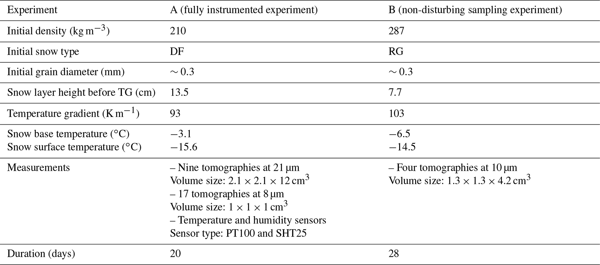
We carried out two experiments that follow the static method to monitor the evolution of a snow layer artificially created in a temperature gradient box. In both experiments, snow profiles are scanned at regular intervals with a DeskTom130 tomograph (RX Solutions) placed inside a cold room at −10 ∘C. In Experiment A, the layer is thicker, leading to a better appreciation of the temperature influence on metamorphism. Temperature and humidity profiles were thus recorded. Since in this experiment the sampling method damaged the lower millimeters, the method was improved in Experiment B: cylindrical samplers, closed at the bottom, were placed in the snow layer at the initial stage and horizontally dug out when needed. An overview of the experimental settings used for both experiments is provided in Table 1.
2.1.1 Experiment A: fully instrumented experiment
Natural fresh snow was collected at Saint-Pancrasse (1000 m, French Alps) in April 2021 and stored at −20 ∘C for 3 weeks. This snow was then sieved using a 1.6 mm diameter sieve in a cold room at −10 ∘C to obtain a horizontal snow slab of 97 cm length, 58 cm width, and 14.5 cm height, composed of decomposing and fragmented precipitation particles (DF) at 210 kg m−3. The snow layer was confined at the base and the top between two copper plates whose temperature was controlled by a thermoregulated fluid circulation. The whole system was insulated with 8 cm thick polystyrene plates. A photograph of the experimental setup and a schematic representation of the top and side view is given in Fig. 1. Isothermal conditions at −10 ∘C were applied to the snow slab for 21 h. This aimed at sintering snow grains whose bonds had been destroyed by sieving. After the isothermal stage, the upper copper plate was lowered by 1 cm to close the gap caused by the snow settling. During the following 20 d, the temperature of the cold room was held at −10 ∘C and the upper and lower copper plates were maintained at −15.6 and −3.1 ∘C, respectively, generating a steady vertical temperature gradient of about 93 K m−1 through the snow layer.
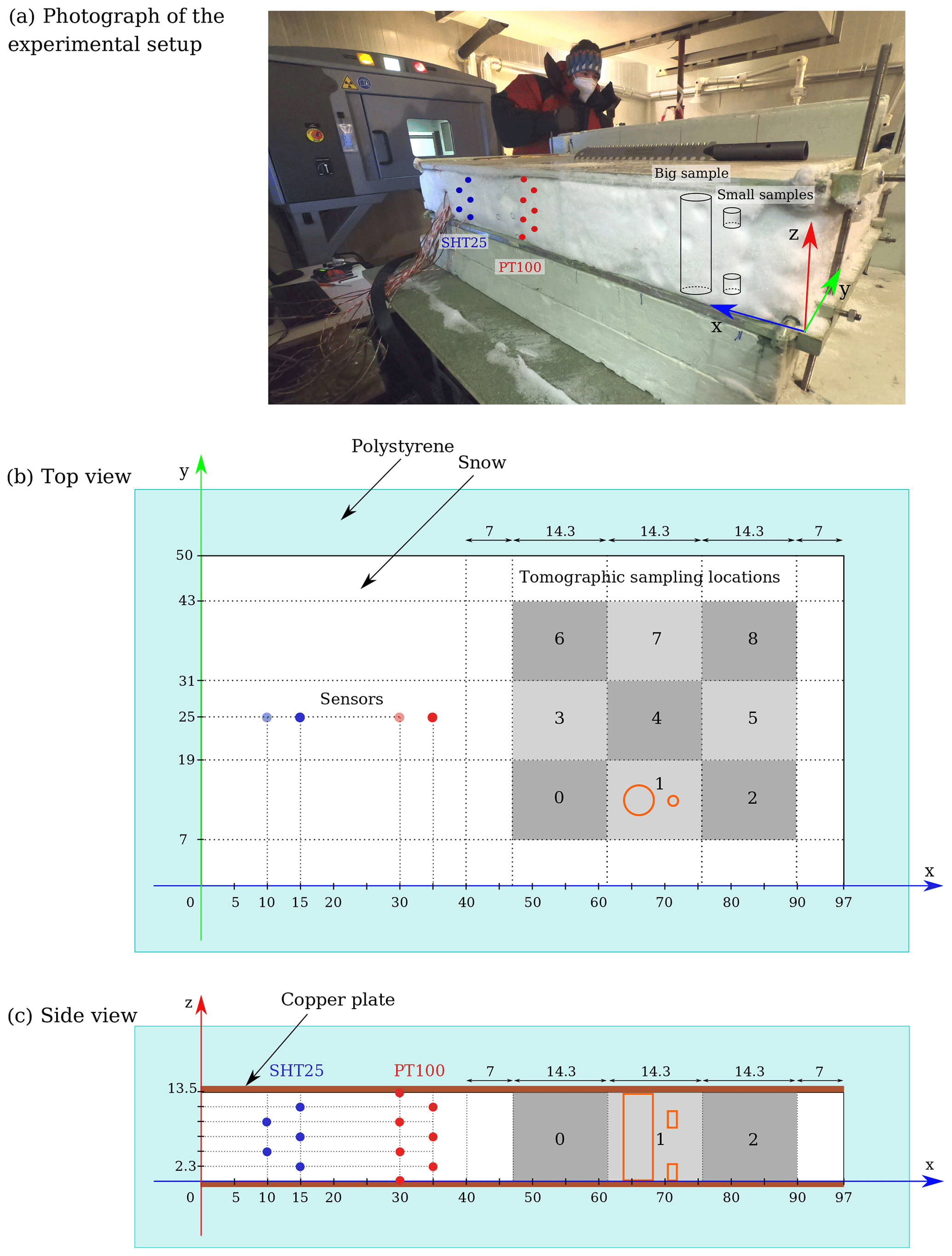
Figure 1(a) Photograph of the experimental setup of Experiment A. (b) Schematic view from above the instrumented box. (c) Schematic view from the side. The locations (in cm) of the two types of sensors are shown with blue and red dots. The tomography sample locations are numbered from 0 to 8 following the chronology of the samplings. The orange contours represent the tomography areas for session 1.
During the sieving process, temperature and humidity sensors were placed in the snow layer at regular heights to obtain two vertical profiles:
-
First is a profile of seven PT100 resistance thermometers made of platinum. Their temperature range varies from −50 to 200 ∘C, they have a 3 mm diameter and are 25 mm long, and their accuracy is ±0.2 ∘C.
-
Second is a profile of five capacitive-type humidity sensors (SHT25, Sensirion). Their dimensions are 3 × 3 × 1 mm3, and their accuracy is ±1.8 % RH.
The SHT25 sensors are marketed with a humidity calibration at ambient conditions (∼ 20 ∘C and ∼ 50 % RH) and present large offsets when placed in cold and humid conditions, up to 7 % RH. A calibration was conducted by placing the sensors in snow to reach close to vapor saturation conditions, in a temperature-controlled box. The applied conditions varied between −4 and −14 ∘C and between 85 % and 100 % RH. A HMP110 (Vaisala) sensor was used as reference humidity value. As the humidity error is correlated to the temperature, a linear correction was applied. In our range of temperature, the correction was between 0 % and 8 %. The capacitive humidity sensors provide relative humidity above liquid water (in %), which is defined as the ratio of the vapor density of the air to the water saturation vapor density. To derive water vapor density (in kg m−3), the following equation was used to obtain the relative humidity above ice:
The Clausius–Clapeyron equation (linking the saturation water vapor density to the temperature) was also used to derive the water vapor density from the relative humidity:
with kg m−3 and Tref=263 K the reference values, J m−3 the latent heat of ice from solid phase to gas phase, kg the mass of a water molecule, ρi=917 kg m−3 the ice density, and J K−1 the Boltzmann constant.
During the 20 d of the experiment, nine tomography sessions were done at regular time intervals. Each consisted of the sampling and scanning of one large sample of the whole vertical dimension and two small samples localized at the top and at the bottom of the snow layer (Fig. 1), leading to a total of 26 samples (only one small sample was collected during the first sampling). For each sampling, the polystyrene plates and the upper copper plate were temporarily removed in order to access the snow slab, disturbing momentarily the upper temperature boundary and breaking the ice bonds between the plate and the snow layer. The samples were vertically extruded at a minimum distance of 7 cm from the edges and from regions already sampled. Large samples were extracted using a polymethyl methacrylate (PMMA) serrated cylindrical core drill with a diameter of 4.5 cm and a height of 14 cm. Small samples were extracted using a copper cylindrical core drill with a diameter of 2 cm and a height of 5 cm. A flat trowel was inserted in contact with the lower copper plate, the cylinder was pushed in the snow layer from the top, and then it was carefully extracted and placed in the tomograph. The very bottom area of the snow was disturbed because of the samplers pressed down in the snow layer, which crushed the grains against the copper plate, and because of the insertion of the flat trowel at the base of the snow layer that destroyed 2 to 3 mm of snow. Holes in the snow layer created by the sampling were systematically refilled with snow to ensure stable temperature and humidity fields. Large samples (around 2.1 × 2.1 × 12 cm3) were scanned with a pixel size of 21 µm. The X-ray tube was powered by a voltage of 60 kV and a current of 260 µA. Small samples (1 × 1 × 1 cm3) were scanned with a pixel size of 8 µm, a voltage of 62 kV, and a current of 129 µA.
2.1.2 Experiment B: non-disturbing sampling experiment
Natural snow was collected at Col de Porte (1325 m, French Alps) in February 2022 and stored at −10 ∘C for 3 d. The snow was then sieved using a 1.6 mm diameter sieve in a cold room at −10 ∘C to obtain a horizontal snow layer of 97 cm length, 58 cm width, and 7.7 cm height, composed of rounded grains (RG) at 287 kg m−3. The same temperature gradient box described in Experiment A was used. During the following 28 d, the temperature of the cold room was held at −8 ∘C. The temperatures of the top and lower copper plates were maintained at −14.5 and −3.5 ∘C, respectively.
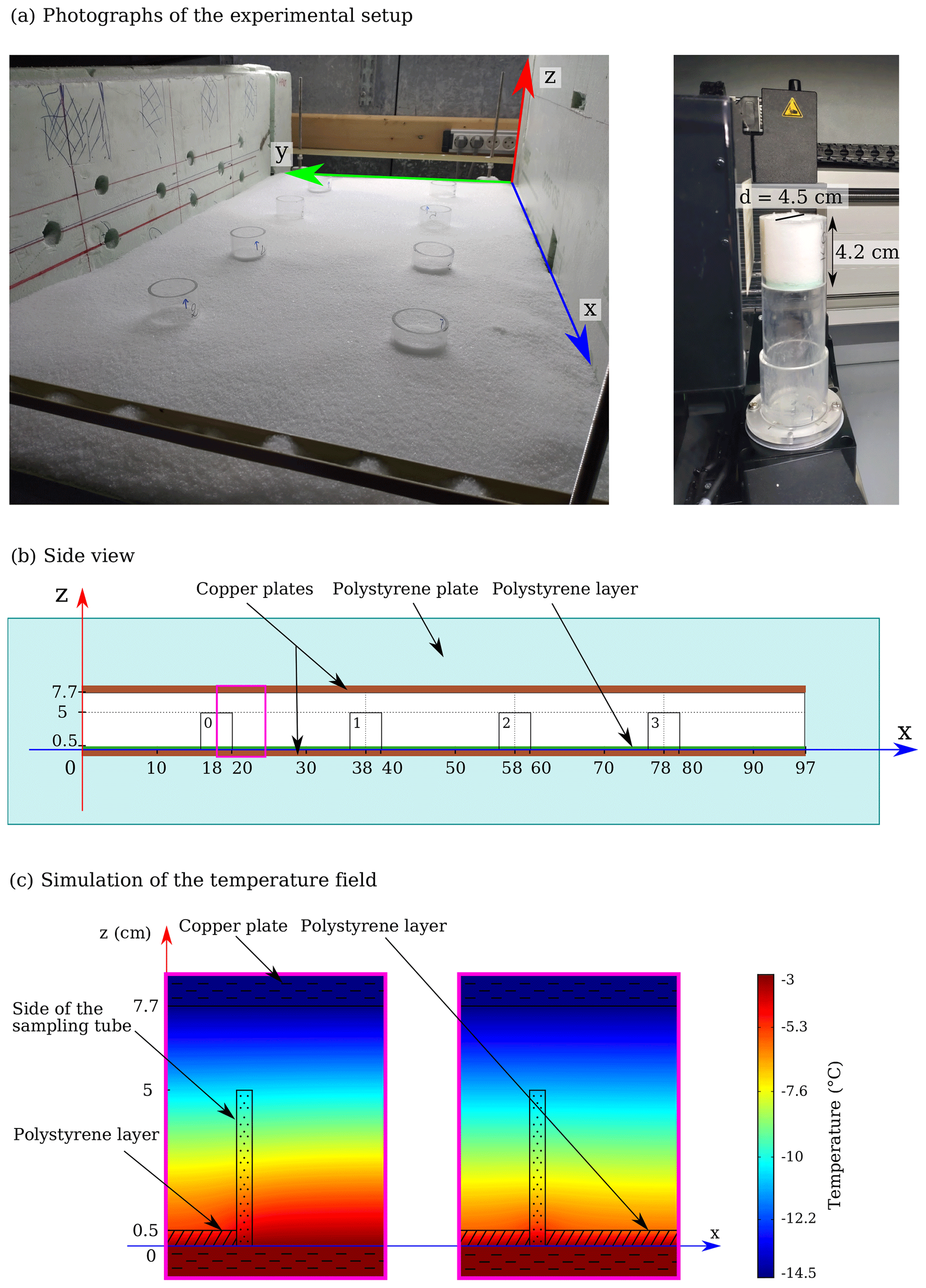
Figure 2(a) Photograph of the experimental setup of Experiment B. (b) Schematic view from the side of the instrumented box. (c) Simulation of the temperature field of the cylinders buried in snow with (left) the polystyrene layer placed only in the cylinders and (right) the polystyrene layer laid on the whole copper plate. The simulated geometry is represented by a pink box in (b) and (c). The simulation was computed with the finite element model COMSOL with axisymmetric conditions.
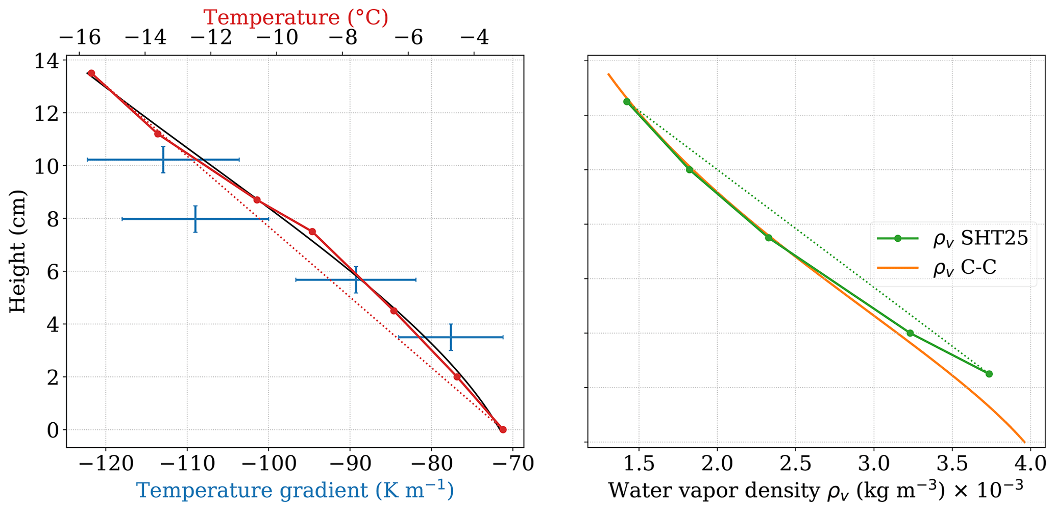
Figure 3Temperature, temperature gradient, and water vapor density profiles during the longest precisely defined steady-condition stage of Experiment A. The black line represents the polynomial fit on the PT100 data. The orange line displays the Clausius–Clapeyron equation applied to the temperature fit. The straight dotted red and green lines, which connect the higher and lower points of the temperature and the water vapor density, respectively, are presented to help highlight the shape of the curves.
For this experiment, the sampling method was improved compared to Experiment A, for which the insertion of the cylinder from the top disturbed the snow, especially at the base of the layer where grains could crush against the copper plate, which prevents analyzing snow at the base. Here, the new method allows us to scan undisturbed snow samples from top to bottom. For that, before snow sieving, eight cylinders made of PMMA with a diameter of 4.5 cm and a height of 4.2 cm were placed on the lower copper plate; the base of the cylinders was closed by a 5 mm thick layer of polystyrene. Cylinders were then filled with snow and buried in the layer during the sieving process. An illustration and a detailed schematic of the experimental setup is given in Fig. 2a and b. The modifications of the temperature field caused by the cylinder and the polystyrene layer were modeled for the initial stage of the snow layer, solving heat transfer equations using the finite element software COMSOL Multiphysics® (Fig. 2c). This figure shows that the setup on the left, with the polystyrene only inside the cylinders, modifies the temperature field. When the whole copper plate is covered with the polystyrene layer, this effect is significantly reduced, as shown in the simulation on the right. In addition, Fig. 2c shows that the presence of the PMMA cylinder does not disturb significantly the temperature field and that non-vertical gradients represent 10 % compared to the vertical ones. Similar results are observed when simulating the end of the experiment with an air gap (12.6 %). With the layer of polystyrene insulating the bottom of the snow, and the upper and lower copper plates maintained at −14.5 and −3.5 ∘C, the temperature was −6.5 ∘C at the snow base above the polystyrene layer, resulting in a temperature gradient of about 103 K m−1 across the snow layer.
Sampling for tomography was performed after 1, 7, 17, and 28 d of the temperature gradient. Each time, two samples were extracted and scanned using X-ray tomography. For sampling, the cylinders, buried in the snow layer, were excavated by digging horizontally from the front of the snow layer and being gently dragged out. The hole was then filled with snow. This method enables sampling without moving the copper plates, and only the front polystyrene plate needs to be temporarily removed. For tomography, the X-ray tube was powered by a voltage of 70 kV and a current of 114 µA. As both samples of each session were visually consistent, only one scan of each day has been analyzed. A total of four scanned samples with a size of 1.3 × 1.3 × 4.2 cm3 and a resolution of 10 µm are presented.
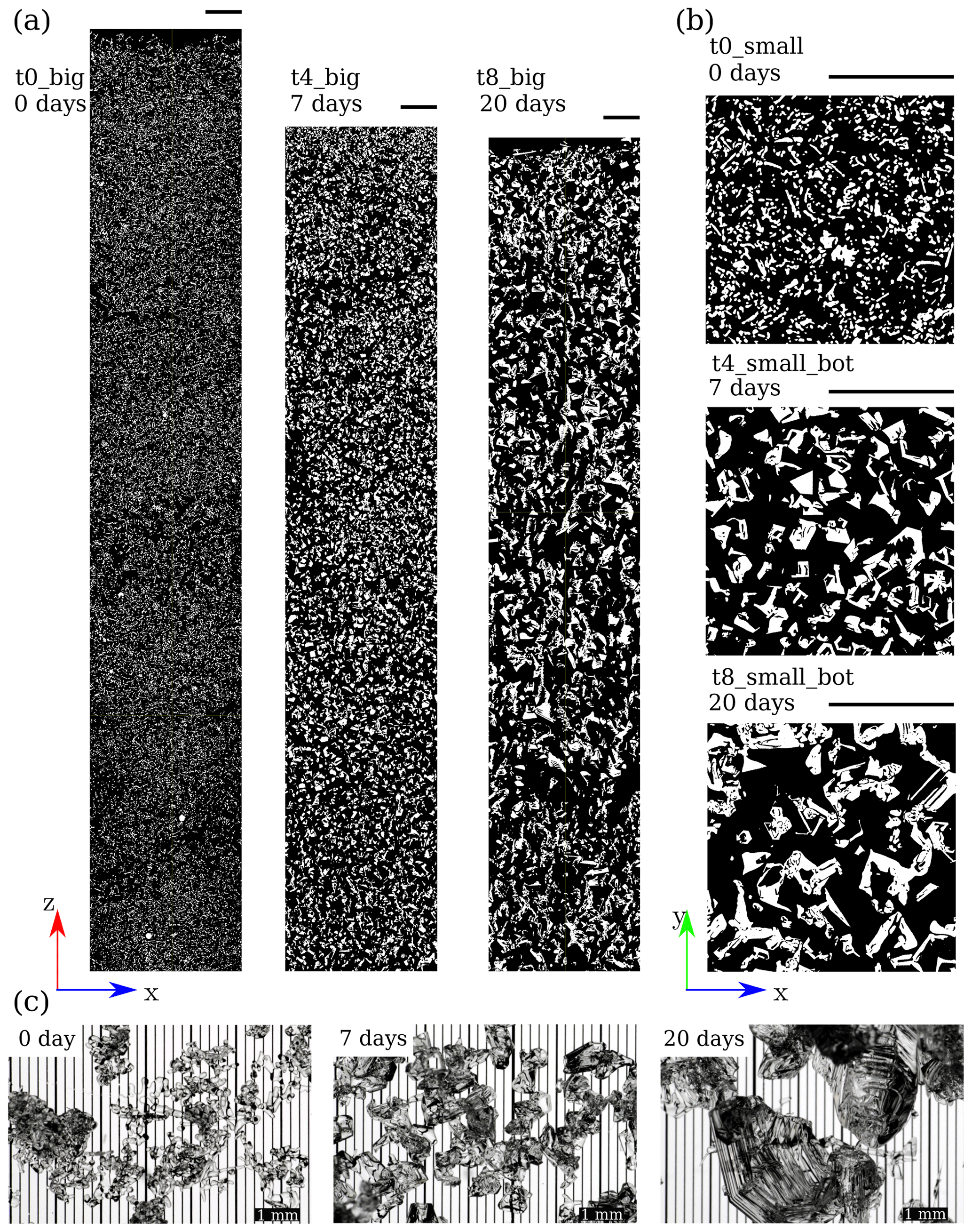
Figure 4(a) Vertical slices of the big samples at 21 µm after 0, 7, and 20 d of Experiment A. (b) Horizontal slices of the small samples at 8 µm. The vertical location of the small samples presented here are, respectively, 8.3, 1.2, and 1.2 cm for the samples at 0, 7, and 20 d. Each scale bar represents 5 mm. (c) Photographs of individual grains from the middle of the layer seen by microscope. All sample names and associated parameters are listed in Table A1.
2.2 3D image processing and analysis
For both experiments, the tomographies were reconstructed into 3D gray-scale images representing the attenuation coefficients of the different materials composing the samples. The ice phase was segmented from the air phase using the energy-based segmentation algorithm developed by Hagenmuller et al. (2013).
Using the segmented 3D images, properties were computed to characterize the microstructural evolution. The snow density ρs (kg m−3) was computed using a simple voxel counting algorithm. The SSA (m2 kg−1), defined as the total surface area of ice per unit of mass, was computed using the voxel projection approach (Flin et al., 2011; Dumont et al., 2021). The covariance (or correlation) length lc, which corresponds to the characteristic size of a heterogeneity made of an ice grain and a pore, was calculated along the x, y, and z directions of the images, as in the work of Calonne et al. (2014). In this study, we use the average of , , and , referred to as the mean covariance length in the following. The structural anisotropy coefficient 𝒜(lc) was computed from the covariance lengths as . The microstructure is considered isotropic when 𝒜(lc) is close to 1 and anisotropic otherwise. 𝒜(lc) values larger than 1 describe a microstructure that is elongated in the vertical direction, and values lower than 1 describe a horizontally elongated microstructure.
For the small samples of Experiment A, properties were computed on the representative elementary volume (REV) of size cm3. The volume of computation of the large samples was around cm3 for Experiment A and cm3 for Experiment B. For those large samples, to observe precisely the vertical mass transfer, the density was computed on each horizontal slice with a running average of 100 voxels applied to the profiles. For SSA, covariance length, and anisotropy parameters, the large samples have been divided into subsamples with the size of the REV of the properties, here cm3 for Experiment A and cm3 for Experiment B.
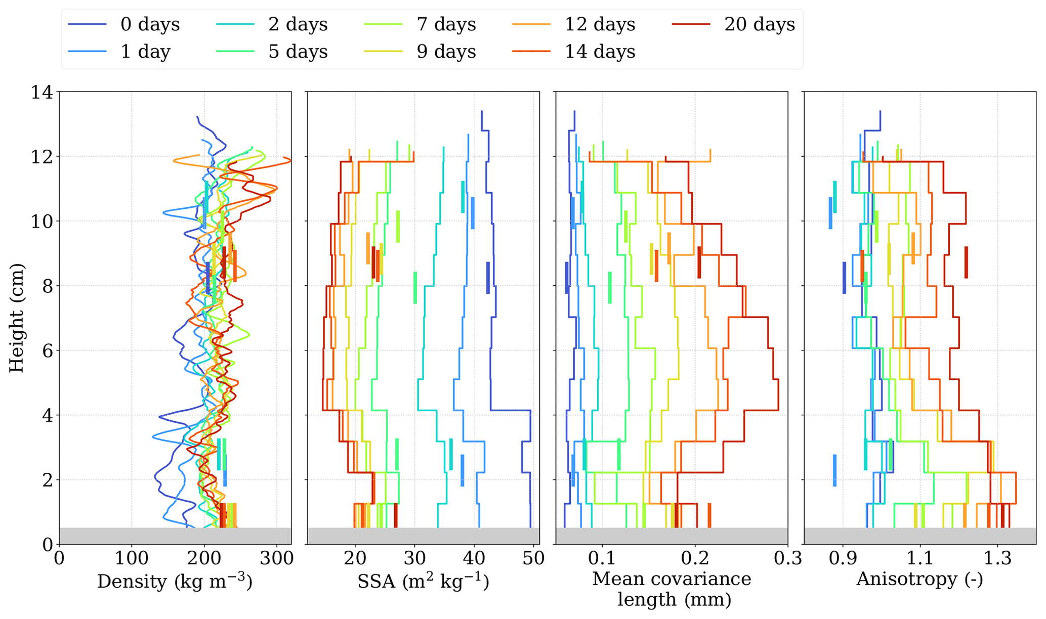
Figure 5Vertical profiles of the microstructural properties of Experiment A. Properties computed from the large samples at 21 µm are shown by step curves and those from the small samples at 8 µm by vertical bars. The density of the samples at 21 µm is computed on each slice with a running average (see Sect. 2.2). The gray area at the bottom represents the disturbed area caused by the snow sampling.
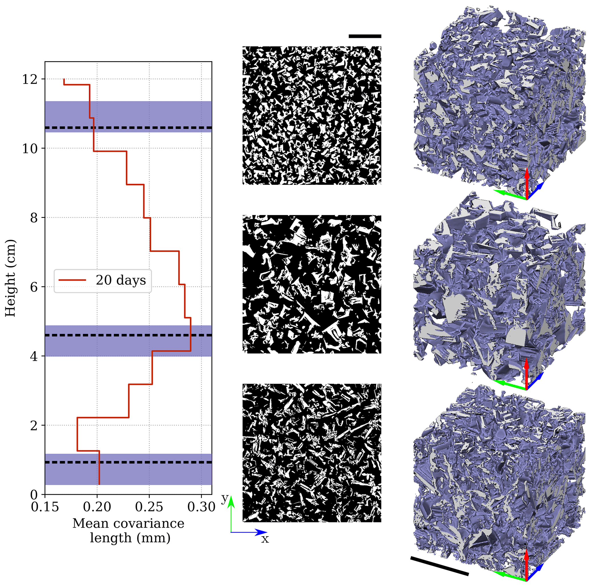
Figure 6Mean covariance length profile, horizontal slices, and 3D subsamples of the large sample at 20 d of Experiment A. Each 3D subsample is 0.95 × 0.95 × 0.95 cm3 and is horizontally centered. The vertical locations of the horizontal slices and of the 3D subsamples are shown, respectively, with dotted black lines and plain violet rectangles on the covariance length profile. The scale bars represent 5 mm.
3.1 Experiment A
3.1.1 Temperature and humidity sensors
The temperature and humidity sensors are used here to monitor the environmental variables of the snow layer. Figure 3 shows the vertical profile of both parameters, which correspond to the average temperature and humidity of the sensors from day 15 to day 17 of the experiment (longest period in steady-state conditions with no sampling). It is worth noticing that after starting the temperature gradient, temperature and humidity reached a stable state after approximately 5 h and remained rather constant for the whole duration of the experiment (variations maximum of 1 % RH and 0.75 ∘C). However, each time the top copper plate was removed to sample the snow layer, the temperature and humidity fields were slightly perturbed for several hours.
The vertical profile of temperature shows a slight upward convex curve, also observed in early experiments (Yosida, 1955; Fukuzawa and Akitaya, 1993; Sturm and Benson, 1997; Kamata and Sato, 2007) and consistent with the prediction of heat and vapor transport models, such as the homogenized model of Calonne et al. (2015b). This upward convex curve is due to the latent heat flux from phase change (sublimation and deposition). Local temperature gradients were calculated by averaging the temperature over a running window of four values. As a result of the curved distribution of temperature, the local temperature gradient is larger on the upper part of the snow layer (∼ 115 K m−1) than in the bottom part (∼ 80 K m−1). A similar and more pronounced result is observed in Kamata and Sato (2007) with local gradients ranging from 1200 K m−1 in the cold part to 300 K m−1 in the warm part, for a macroscopic gradient of 530 K m−1.
The vertical profile of water vapor density shows an upward concave curve due to the nonlinear dependence between the temperature and the saturation vapor density and due to the vapor sources and sinks. In the figure, the Clausius–Clapeyron equation applied to the polynomial fit of the PT100 profile (in black in the temperature plot) is shown in orange. It presents a two-point inflection curve, which is the consequence of the upward convex temperature profile (Sturm and Benson, 1997). The measured humidity profile is very close to the saturation vapor density in the upper half and deviates from it in the lower area. The difference between the two curves can be expressed in terms of supersaturation (), which reaches σ=0.24 g m−3 for the lower point. However, further quantitative analysis of the supersaturation is not feasible due to the poor resolution of the profile and of the uncertainty of our humidity measurements.
3.1.2 Qualitative analysis of the tomographs
Figure 4 presents, in a qualitative way, the microstructural evolution of snow during the 20 d of the temperature gradient. Vertical slices of the snow column of the large samples at 21 µm and horizontal slices of the small samples at 8 µm taken at 0, 7, and 20 d are shown, as well as the associated photographs of grains. The microstructure gradually transforms from decomposing and fragmented precipitation particles (DF) towards DH, and grains and pores are getting larger. Photographs of grains taken with a microscope show the detailed features of the grains, such as the rounded dendrites at day 0, the facets and angular shapes at day 7, and the large hollow striated cup shapes arranged in vertical chains after 20 d. The type of depth hoar obtained at the end of the experiment is standard depth hoar (formerly called skeleton-type depth hoar; Akitaya, 1974; Fierz et al., 2009).
3.1.3 Microstructural properties
Figure 5 presents the vertical profiles of microstructural properties. The small samples are presented in the figure with small vertical bars. The gray area represents the disturbed area at the base of the snow layer caused by the sampling method (see Sect. 2.1.1).
First, the effect of resolution on the property computations, using both the large samples at 21 µm and the small samples at 8 µm, can be observed. Precise comparisons are however challenged by the superimposing influence of the spatial variability, which creates variations between samples collected at the same time but at locations slightly different in the layer. Overall, the properties of the small and large samples are of the same order of magnitude, with average differences of 5 % for the density, 15 % for the SSA, 6 % for the covariance length, and 2 % for the anisotropy parameter.
Looking at the evolution of the properties in time, the density evolution suggests the settling of the snowpack in the first days of the experiment with a slight increase in the density and the loss of about 1 cm height. This rapid settling is mainly due to the isothermal phase before the temperature gradient. After the first 2 d, the density remains stable to the end of the experiment. The SSA decreases overall with time, with mean vertical values evolving from 44.5 to 17.5 m2 kg−1 after 20 d. Consistently, the mean covariance length increases gradually with time so that the characteristic size of heterogeneities is tripled, from 0.07 to 0.23 mm (mean vertical value). The anisotropy coefficient 𝒜(lc) increases in time to reach values around 1.2 after 20 d, reflecting the typical elongation of the ice structure along the vertical temperature gradient direction (grain chains).
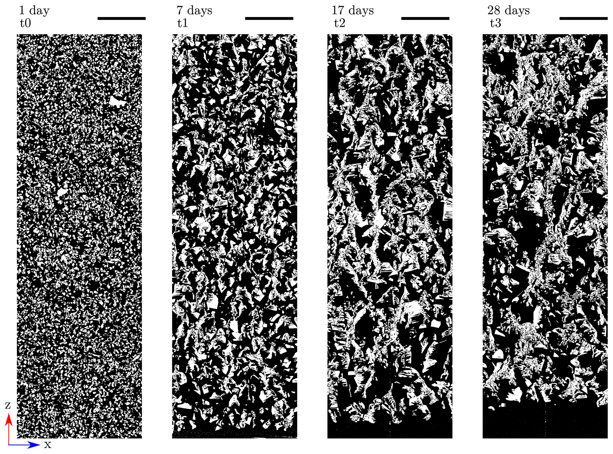
Figure 7Vertical slices of the four samples of Experiment B. Each scale bar represents 5 mm. All sample names and associated parameters are listed in Table A1.
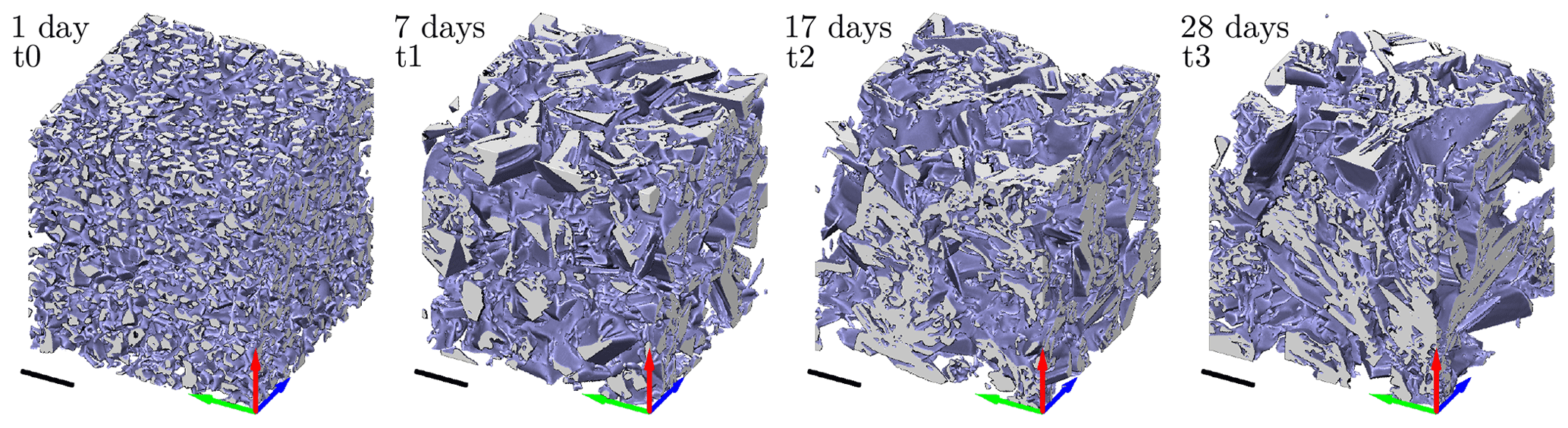
Figure 8The 3D representations of subsamples of Experiment B. Each subsample is 0.44 × 0.44 × 0.44 cm3 and shows the central part of the imaged snow column. Each scale bar represents 1 mm.
Then, the evolution of the properties along the vertical dimension is analyzed. The overall density remains constant along the vertical, around 220 kg m−3, although significant initial vertical variability can be observed, mainly caused by the sieving process. Specifically, no density drop is observed at the bottom (taking into account that the snow base could not be imaged – see Sect. 2.1.1). It gets more interesting when looking at SSA and covariance length profiles. Lower SSA, down to 14.5 m2 kg−1, and greater covariance length, up to 0.29 mm, are found in the middle part of the snow layer and stand out compared to values in the top and the bottom parts. As these vertical variations are not present at the initial stage, it indicates that the snow microstructure transforms in a different way within the snow layer – more precisely that the size of the ice and air heterogeneities develop a non-monotonous vertical distribution during the experiment. To analyze these differences further, Fig. 6 shows the final state with horizontal slices and 3D views of the snow microstructure in the top, middle, and bottom parts of the layer, together with the covariance length profile. At the top, snow consists of numerous small grains with solid-type crystals (lower covariance length and intermediate SSA). In the middle, larger sparse grains dominate (higher covariance length and lower SSA). At the bottom, grains are smaller, are more elongated, and show complex entangled dendritic crystals (lower covariance length and higher SSA). This last type of morphology is also characteristic of high-supersaturation conditions, which is supported by Fig. 3. This outcome will be further discussed in Sect. 4.1.
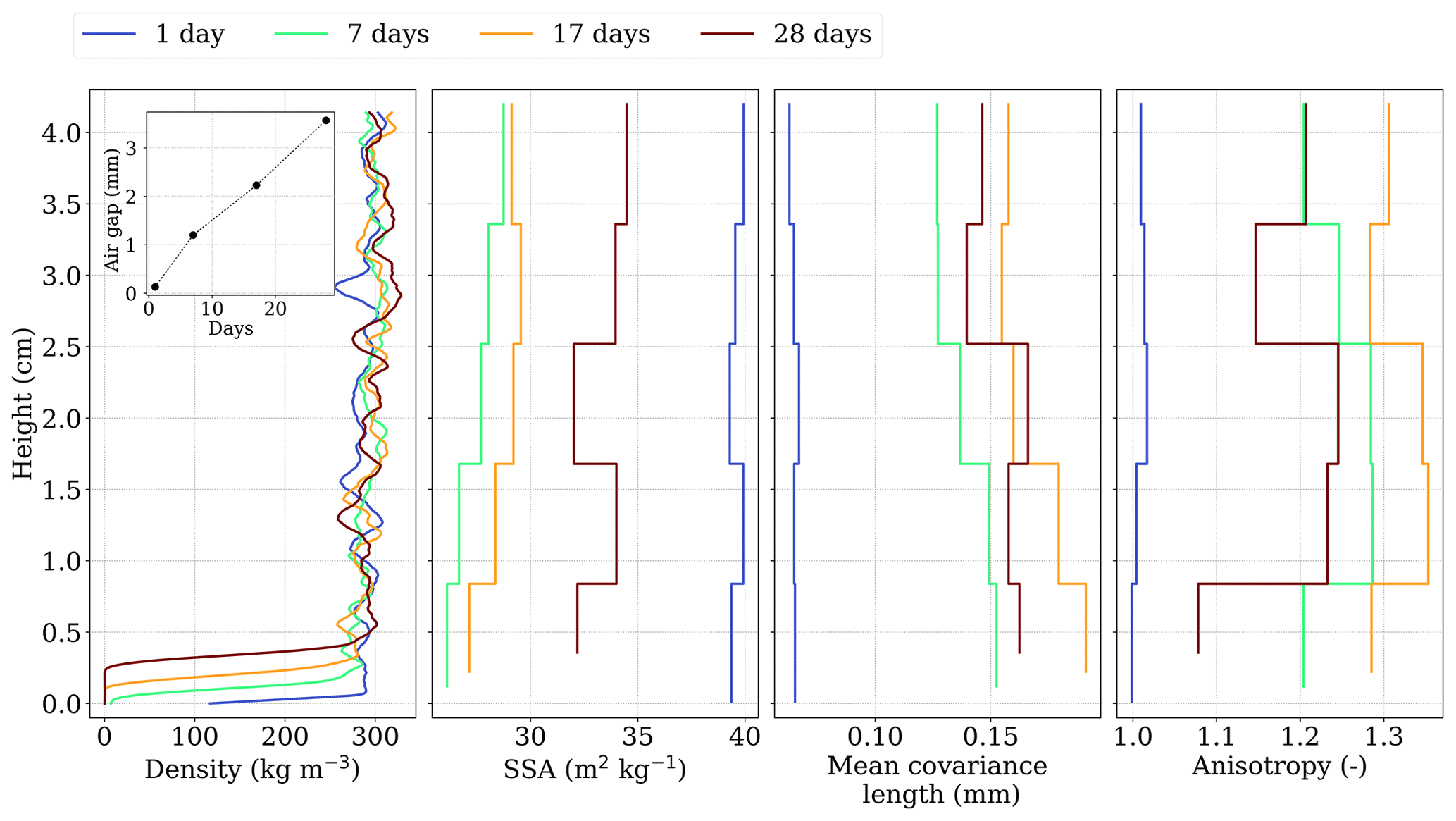
Figure 9Evolution of the vertical profile of the microstructural properties over time during Experiment B. The evolution of the air gap thickness is displayed in the subpanel.
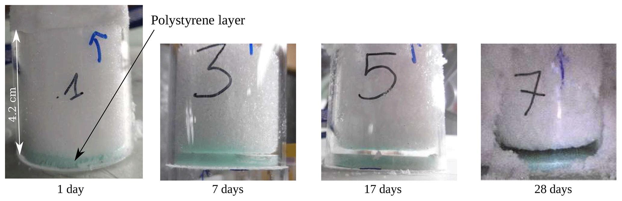
Figure 10Pictures of the snow samples collected at different times from the snow layer during Experiment B. The development of the air gap can be seen at the sample base.
3.2 Experiment B
3.2.1 Qualitative analysis of the tomographs
A visualization of the microstructural evolution is shown in Fig. 7 with vertical slices of the segmented images and in Fig. 8 with 3D views of centered subsamples. As the snow evolves, one can clearly see the transformation from the first step (after 1 d of temperature gradient), presenting dense FC to DH at 7 d, and finally to the last stages at 17 and 28 d where vertical structures appear and dendritic features develop. The last stage can be characterized as hard depth hoar, which has been previously described as a dense and cohesive structure, with hoar crystals connected by necks and vertical grain-to-grain chains (Akitaya, 1974; Pfeffer and Mrugala, 2002). A hand hardness test was conducted and showed hardness classified as “pencil”, corresponding to a high resistance to penetration (Fierz et al., 2009). Figure 7 also provides a clear insight of the local mass loss at the bottom of the samples, as an air gap gradually forms. Here, unlike in Experiment A, the base of the snow column could be scanned, and it provides an accurate observation of the bottom interface, as seen in the images.
3.2.2 Microstructural properties
As for Experiment A, Fig. 9 presents the evolution of the vertical profile of the microstructural properties with time. In terms of overall temporal evolution, the SSA shows a large decrease for the first days of the experiment, dropping from 39.6 to 27.5 m2 kg−1 after 7 d, followed by an increase during the remaining time, up to 33.3 m2 kg−1 at the end of the experiment. This increase in SSA can be seen as a specificity of hard depth hoar and will be further discussed in Sect. 4. The evolution of the covariance length takes place mainly during the first week, where values increase from about 0.07 to 0.14 mm in 7 d. Similar covariance lengths, around 0.15–0.16 mm, are then found until the end. This evolution of the size of the heterogeneities can also be observed in Figs. 7 and 8, with a drastic change in the microstructure in the first step, while the microstructure between 17 and 28 d does not show such a pronounced change. Similarly, the anisotropy 𝒜(lc) increases strongly in the first time step and seems to reach a stable range after 7 d. Considering the full height, the average density of the samples decreases from 287 to 273 kg m−3, indicating a regular mass loss of 5 % for each consecutive time step.
In terms of vertical variations, density shows the most significant evolution. A sharp drop in density localized in a thin layer at the bottom of the samples is observed. This air gap between the green polystyrene layer and the snow can be seen from the pictures of the snow samples presented in Fig. 10 and by the growing black area at the bottom of the segmented images in Fig. 7. We define the top boundary of the air gap as the height where snow reaches a density of 200 kg m−3. The evolution of the air gap thickness shows a linear progression from 0.1 to 3.6 mm (subpanel in Fig. 9). By a visual inspection, we noted that this air gap developed at the whole base of the snow slab and not only in the cylinders. Finally, SSA and covariance length show a slight slope in their vertical profile that seems to develop over time (Fig. 9). From top to bottom, SSA tends to decrease and covariance length tends to increase, meaning that grains become slightly larger towards the bottom.
4.1 Vertical evolution of the grain morphology
In Experiment A, different grain morphologies develop over time along the vertical, with coarser grains and pores in the middle characterized by higher covariance length and SSA (Figs. 5 and 6). This distribution was not present at the initial stage and formed during the TGM. To further quantify the evolution of the size of the ice and air heterogeneities in the vertical direction, a growth rate was calculated at different heights by dividing the difference between the initial and the final covariance lengths by the duration of the experiment (Fig. 11a). This lc-based growth rate depicts the growth of the air and ice structure at the REV scale. As expected, the growth rate also shows a non-monotonous distribution with a maximum in the middle part at 9.4 × 10⁻¹¹ m s−1. As a comparison, during the experiment of Kamata and Sato (2007), the growth rate increased linearly from 0 m s−1 at the top of the snow layer at −70 ∘C to 8 × 10⁻¹⁰ m s−1 at the bottom at −10 ∘C.
The more intense growth found in the center part is surprising as it does not follow the well-known dependency between metamorphism rate and temperature: the warmer the temperature, the more active the metamorphism (e.g., Kamata et al., 1999; Kamata and Sato, 2007). In our case, the largest grains would have been expected at the warmer bottom and the smallest grains at the colder top, with a monotonous grain size distribution across the snow layer. Thus, temperature alone cannot explain our results. Other known impacting factors are the temperature gradient intensity and snow density. As seen in Figs. 3 and 5, both parameters show a monotonous vertical distribution and cannot be the cause of the observed vertical heterogeneities.
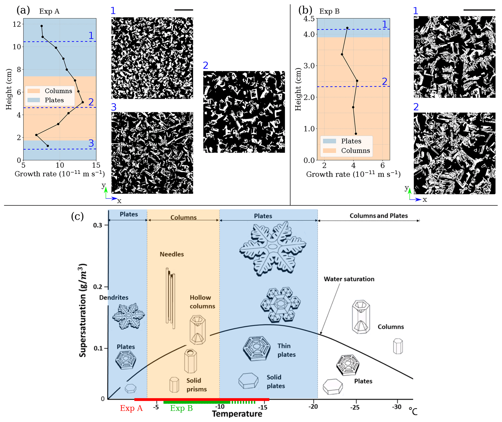
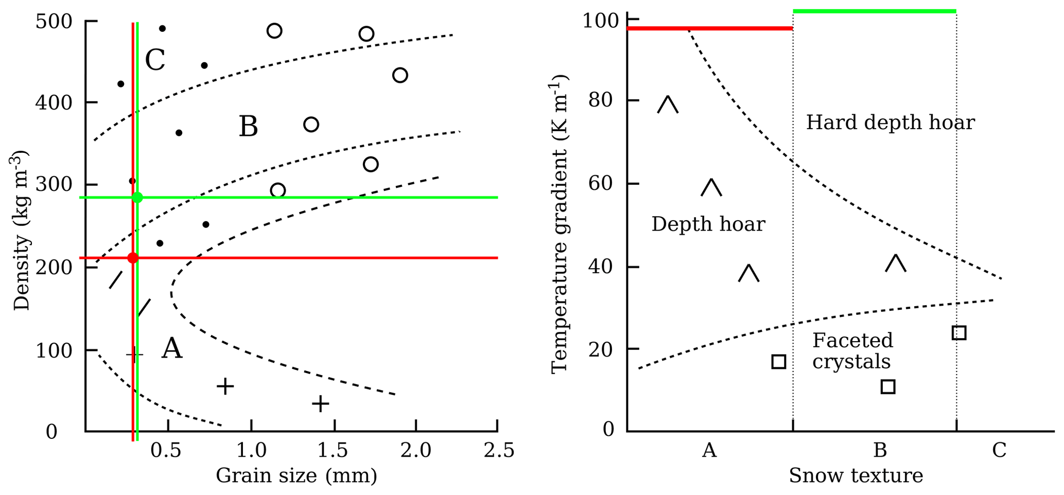
Figure 11(a) Growth rate and horizontal slices at different heights of the sample at 20 d for Experiment A. (b) Growth rate and horizontal slices for Experiment B. (c) Nakaya diagram (adapted from Libbrecht, 2021) with colors representing the basal (orange) and prismatic (blue) regimes. On the temperature axis, the red line corresponds to the temperature range of Experiment A and the green line to the one of Experiment B (the dotted line represents the snow above the scanned sample).
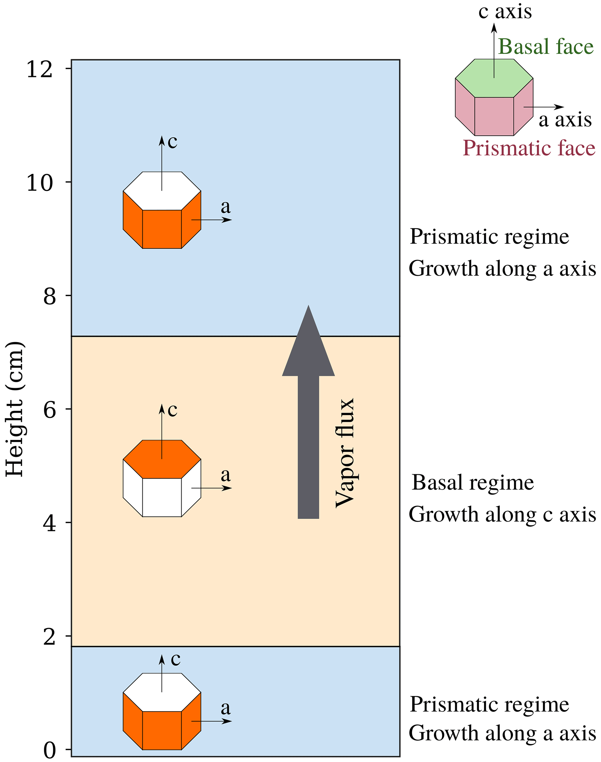
Figure 12Simplified representation of grain growth configuration in the case of vertical c axes for Experiment A.
One hypothesis to explain the observed variations within the layer is the effect of the different regimes of crystal growth as a function of temperature. Ice crystals grow preferentially depending on temperature either along the c axis (basal regime) or along their a axes (prismatic regime). Those preferential growth regimes are illustrated in the Nakaya diagram in the case of growing ice crystals in the atmosphere (Fig. 11c), where either column-like crystals or plate-like crystals are obtained. Experiment A covers temperatures from −3.1 to −15.6 ∘C (in red in Fig. 11) and comes across different regimes of the Nakaya diagram: from prismatic (in blue), to basal (in orange), and again to prismatic from the bottom to the top of our snow layer. Interestingly, when overlapping the regimes and the growth rate profile, the variations in the profile seem to match with the three regimes (Fig. 11a). The highest growth rates coincide with the basal regime, whereas smaller values are found rather in the prismatic regime. In terms of microstructural features, different morphologies are observed in the prismatic and basal regimes.
Former studies already pointed out a link between crystal growth regime and the shape of snow grains in the snowpack. Akitaya (1974) suggested that crystal regimes influence the shape of depth hoar. Based on micro-photographs, the author observed a dependence of temperature on the depth hoar habits, such as needle-like grains at −5.1 ∘C and plate-like grains at −2.2 ∘C, which is in agreement with the Nakaya diagram. In terms of field observations, Sturm and Benson (1997) investigated the vertical sequence of snow texture in a subarctic snow cover using a microscope and photographs. In the lower part of the snowpack, they reported two layers that showed opposite characteristics with rather plate shapes or columnar shapes, which could be attributed to prismatic and basal growth, respectively.
To explain how basal growth could have caused the observed enhanced grain growth in the center of the layer, we suggest a scenario involving the crystal orientation of the ice grains (see Fig. 12). During the sieving phase, the snow was composed of recent snow (DF) showing many plate-like crystals. Riche et al. (2013) suggested that such crystals tend to deposit with their c axes preferentially vertically oriented because of their shapes. In our case, this would lead to numerous grains having their c axes oriented close to the vertical axis. A higher proportion of basal surfaces would thus face the vertical vapor flux compared to the prismatic faces. Hence, in the center of the layer where basal growth is favored, those basal surfaces would grow actively as they benefit from both a high vapor intake and enhanced phase change. In comparison, in the upper and lower part, where prismatic growth is favored, prismatic surfaces do benefit from enhanced phase change but not from a high vapor intake, as they do not face the vapor flux. It would result in the formation of larger grains in the center part of the snow layer in comparison to the top and bottom. A similar orientation-selective metamorphism has been observed by Granger et al. (2021) between −4 and −2 ∘C for prismatic faces: based on diffraction contrast tomography and interface tracking, they showed that prismatic preferential growth occurred, with higher sublimation and deposition rates, for grains with their c axes close to the horizontal plane. This observation was actually realized from a nearly isotropic initial distribution of c axes. In fact, without considering the initial orientation of the c axes in our experiment, the temperature range effect would probably also lead to a selection of vertical c axes between −4 and −10 ∘C and to horizontal c axes elsewhere, thus differentiating the observed morphologies.
Unlike Experiment A, Experiment B shows a growth rate and a covariance length profile that do not show any clear bump and are rather monotonous (Figs. 9 and 11b). In Experiment B, the temperature range varies from −14.5 to −6.5 ∘C in the snow layer and from −11 to −6.5 ∘C inside the samples, meaning that most of the scanned snow underwent temperature conditions that fall into the basal regime. In terms of magnitude, the growth rate is lower in Experiment B than in Experiment A. This can be related to the density, higher in Experiment B than in Experiment A, as grain growth is more constrained in space in dense snow so that smaller grains form (e.g., Akitaya, 1974; Granger et al., 2021).
Superimposing the temperature range effect, supersaturation can also play a role in the grain morphology. As illustrated with the vertical axis of the Nakaya diagram (Fig. 11c), grains show more complex shapes such as dendritic and hollow structures in conditions of high supersaturation. As seen in our measurements in Fig. 3, the bottom area of the snow layer shows high-supersaturation conditions, which could indicate a rapid growth of small and complex features while keeping the mean covariance length rather small. This is supported by the final morphology of this area shown in Fig. 6.
In light of both experiments A and B, it seems that specific conditions must be fulfilled to observe the formation of heterogeneities within an initial homogeneous snow layer under TGM that would be caused by the crystal growth regimes. First of all, the temperature range should cover multiple growth regimes, which is easier to maintain in laboratory than in natural conditions, where the upper temperature is constrained by the changing atmospheric temperature. The initial density appears to play a role: low-density snow enables conditions closer to those encountered in the atmosphere, as crystal growth is not restricted by the proximity of other grains, whereas high-density snow constrains the condensation process on a shorter scale (Granger et al., 2021).
The processes described here happen within several centimeters inside the snowpack and impact greatly the microstructural properties such as the covariance length and the SSA while keeping the density nearly constant. From an initial homogeneous snow layer, the temperature and vapor density conditions lead to considerable heterogeneities in the layer microstructure. To describe a natural snowpack undergoing temperature gradient conditions, considering those processes could have a significant impact on macroscale models such as Crocus (Vionnet et al., 2012) and SNOWPACK (Lehning et al., 2002). For instance, the thermal conductivity is at first order driven by the density, but Calonne et al. (2011) have shown that it is also dependent on the microstructural arrangement. Similarly, the mechanical behavior of the snowpack could also be impacted by heterogeneities in the grain morphologies of a snow layer (see, e.g., Hagenmuller et al., 2014; Wautier et al., 2015).
4.2 Basal mass loss
An important part of this study is the monitoring of the mass loss in the first millimeters of the snow layer, made possible by the non-disturbed sampling method of Experiment B. The standard sampling method, as used in Experiment A, does not provide reliable data on the bottom area of the snow (see Sect. 2.1.1). Moreover, the removal of the top copper plate disturbed the temperature field. In contrast, in Experiment B, the copper plates remained in place and the contact with the snow was insured during the whole experiment, as the samplers were extracted from the snow layer from the side of the temperature gradient box.
The air gap on the base of the sample reached 3.6 mm, along with a mass loss of 5 % of the initial ice, in 28 d for a temperature gradient of about 100 K m−1 and temperatures near −6.5 ∘C. As only the first 4 cm of the snow layer (7 cm total height) was sampled and scanned, the mass redistribution in the upper part of the snow layer cannot be observed. This air gap was caused by the continuous mass transfer from the warm bottom to the cold top through the processes of diffusion and phase changes. For comparison, in the extremely high-temperature-gradient experiment of Kamata and Sato (2007), mass transfer was studied for a snow layer of 10 cm by weighing the mass of sublayers of 2.5 cm height each. The density of the lower sublayer decreased from 166 to 152 kg m−3 in 5 d under a local gradient of 270 K m−1 and an averaged temperature of −16 ∘C, whereas the other three sublayers showed a slight increase of 2 to 4 kg m−3 under gradients ranging from 480 to 700 K m−1 and averaged temperatures from −26 to −56 ∘C. As the vertical resolution was 2.5 cm, it is difficult to know whether a localized air gap formed, like in our experiment. Wiese (2017) monitored by in vivo tomography the evolution of a snow sample laying on an artificial frozen soil (frozen glass beads) under a 100 K m−1 gradient. After 21 d, they observed the formation of a low-density layer of 2 to 3 mm, as well as the partial drying of the soil. In terms of field observations, Domine et al. (2019) reported a gradual density drop of the first 10 cm at the base of the arctic snow cover from 400 to 160 kg m−3 for snow that underwent about 4 months of a temperature gradient between 30 and 50 K m−1. In comparison to the gradual decrease they observed, our results show a very abrupt mass loss with a thin layer completely empty of ice (maintained by the upper plate and the sides of the gradient box and the sampling tubes), which may be due to the dry condition imposed at the bottom ensuring no source of water vapor from underneath.
Depending on the soil nature and humidity, an abrupt or more gradual less dense layer can be formed. Wiese (2017) showed that even for soils containing a large proportion of ice, a low-density layer can appear. A cavity of several centimeters on the whole base of the snow cover could hold in spite of gravity with the topography or the vegetation making bridges on the snow base. As suggested by Domine et al. (2019), this drop in density at the ground interface could have a major influence on macroscale snow models such as Crocus and SNOWPACK in terms of mechanical processes and heat and mass transfer properties. In this regards, the data provided, which include quantification of the mass loss as well as the well-constrained forcing conditions, can contribute to evaluate mass transfer models.
4.3 Hard depth hoar observation
When comparing the microstructure obtained at the end of experiments A and B, very different features can be observed. In Experiment A (Fig. 4), the final microstructure is standard (skeleton-type) depth hoar, which is known to be fragile. In Experiment B (Figs. 7 and 8), the final microstructure corresponds to hard (or cohesive) depth hoar, as confirmed by the hand hardness test. Another difference between experiments A and B is the trend in SSA. In Experiment B (Fig. 9), the SSA decreases in the first week and then increases for the following 3 weeks, whereas in Experiment A (Fig. 5), the SSA decreases during the whole period. The increasing trend of SSA is evidence of hard depth hoar development, as the rapid sublimation and deposition rate on a dense structure results in very dendritic and intricate structures that tend to increase the SSA with more complex shapes, as opposed to the typical logarithmic decrease in SSA reported in most of the metamorphism studies (e.g., Cabanes et al., 2003; Flin et al., 2003; Domine et al., 2009). The trend in the SSA for the development of hard depth hoar is thus controlled by two opposite mechanisms, grain growth and the formation of complex surfaces (Wang and Baker, 2014).
In terms of morphology, Akitaya (1974) reported that the three main factors that determine whether TGM will produce hard depth hoar are the initial density, the initial snow type (and grain size), and the temperature gradient. Following this concept shown in Fig. 13, the initial conditions of Experiment A (DF, grain size ≃0.3 mm, ρs=210 kg m−3, TG = 93 K m−1) could likely lead to standard depth hoar, whereas the initial conditions of Experiment B (RG, grain size ≃0.3 mm, ρs=287 kg m−3, TG = 103 K m−1) would lead to hard depth hoar.
Following Wang and Baker (2014), who studied the formation of hard depth hoar for low-density snow, we showed that hard depth hoar can form not only with an extreme temperature gradient or very dense snow but also under more standard conditions with a rather strong gradient of 100 K m−1 and a density of 287 kg m−3. Hard depth hoar presents specific mechanical properties with a cohesive structure compared to the typical depth hoar, making its prediction and identification valuable, for instance, for avalanche risk forecasting.
This study focuses on two features of strong temperature gradient metamorphism at the scale of a snow layer: heterogeneous grain growth and vertical mass transfer. For that, two cold-room experiments were performed to monitor the evolution of a snow layer held under a 100 K m−1 temperature gradient, based on regular snow sampling and imaged by X-ray tomography. Temperature and humidity profiles were recorded during the first experiment to monitor the environmental conditions of the snow layer. We report that, from an initially homogeneous snow, strong heterogeneities developed across the thickness of the snow layer. Coarser and more solid grains developed in the middle of the layer compared to the top and bottom part, as shown by a covariance length about 3 times higher and a lower SSA. Transitions in microstructure seem to match with transitions in crystal growth regime (Nakaya diagram). Indeed, snow is subjected to temperatures that favor, from bottom to top, prismatic, basal, and prismatic growth regimes. The effect of the supersaturation was also highlighted by complex ice features in the bottom, where high supersaturation was measured. The other significant vertical signal was the basal mass loss, observed thanks to a non-disturbing sampling method. An air gap of more than 3 mm formed in 28 d. This drastic mass loss was caused by the vertical vapor flux and accentuated by the dry boundary conditions imposed at the bottom. Finally, from two similar experiments, hard depth hoar was observed in the second experiment characterized by higher initial density. Hard depth hoar was identified through a hand hardness classified as “pencil” and showed an increasing SSA with time, as opposed to the typical trend.
Our results show that a temperature gradient can form heterogeneities within an initially homogeneous layer, regarding mass and morphology. As a consequence, macroscale processes such as heat transport or mechanics may also be impacted. Hence, it could be important to include these temperature gradient features in snowpack models to refine the description of the metamorphism, transport properties, and mechanical behavior. To go in this direction, our measurements, composed of tomographic time series associated with temperature and humidity profiles, constitute a valuable evaluation dataset with well-constrained conditions and quantified evolution. Specifically, the temperatures and mass distributions could be used to evaluate heat and mass transfer models. Humidity profiles are more challenging to measure, and additional development should be done to obtain more robust data for comparison, especially for the evaluation of precise vapor fluxes and supersaturation. To further quantify the basal mass loss, a systematic study could be done, considering the intensity of the temperature gradient and the soil moisture influences. Complementary studies should be done to test the hypothesis provided for the heterogeneous depth hoar growth, adding crystalline orientation measurements for instance. Another interesting possibility would be to find suitable field conditions, such as the high temperature gradients of the arctic snowpack, to look for evidence of these heterogeneities.
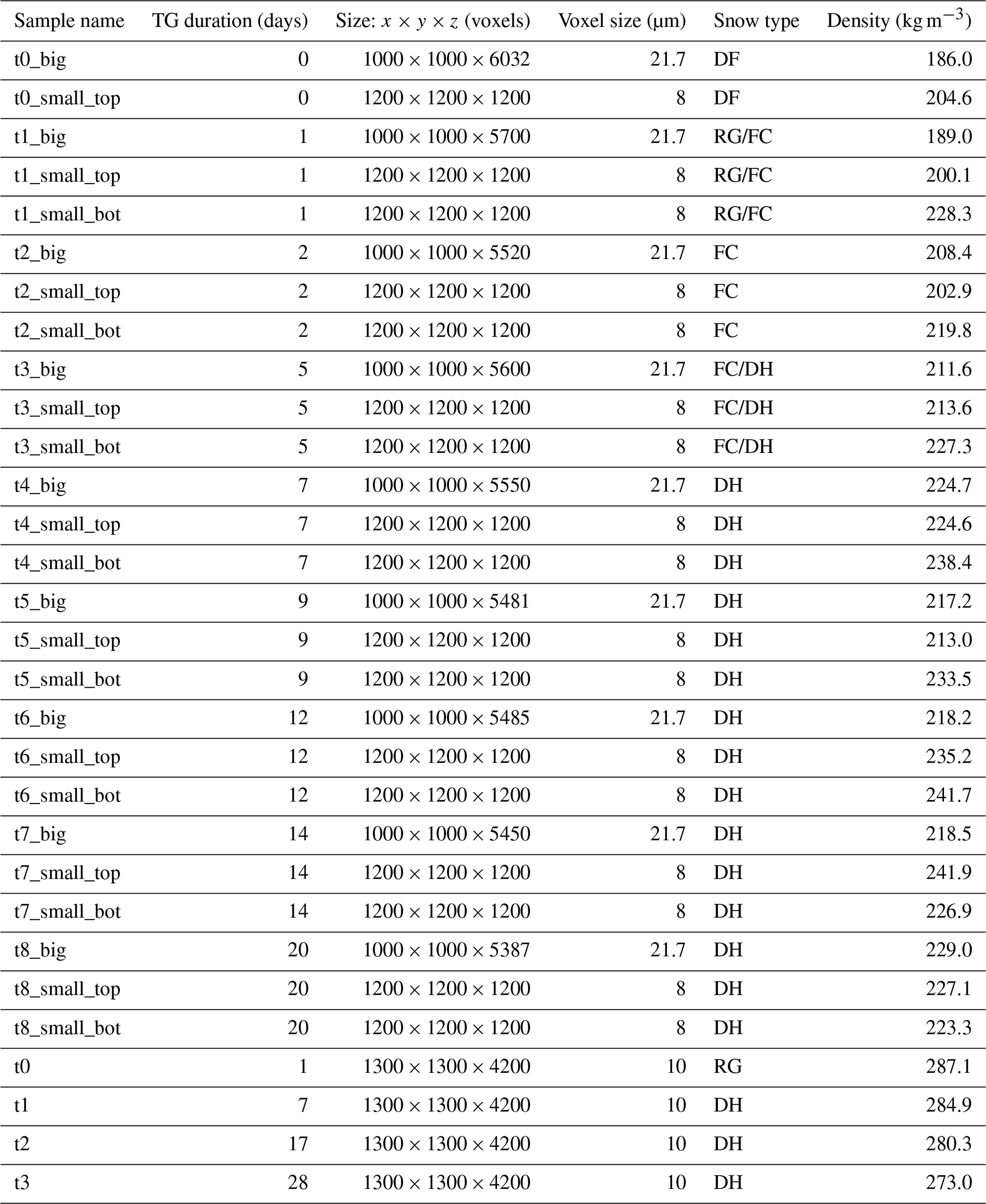
Table A1List of the 30 tomographic images used in experiments A and B (upper and lower parts of the table, respectively). Snow types are given according to the international classification (Fierz et al., 2009).
The data generated and investigated in this article are available in the Supplement.
The supplement related to this article is available online at: https://doi.org/10.5194/tc-17-3553-2023-supplement.
LB and NC designed the experiments and carried them out. The data were analyzed and interpreted by LB with the help of FF, NC, and CG. LB prepared the manuscript with contributions from all co-authors.
The contact author has declared that none of the authors has any competing interests.
Publisher’s note: Copernicus Publications remains neutral with regard to jurisdictional claims in published maps and institutional affiliations.
The authors would like to acknowledge the two anonymous reviewers, along with the editor Jürg Schweizer, for their constructive suggestions which led to the improvement of this paper. The authors also thank Laurent Pezard and Jacques Roulle for their help during the experiments.
The tomography apparatus (TomoCold) was funded by INSU-LEFE, Labex OSUG (Investissements d’avenir, grant ANR-10-LABX-0056), and the CNRM. The 3SR lab is part of the Labex Tec 21 (Investissements d’Avenir, grant ANR-11-LABX-0030). CNRM/CEN is part of Labex OSUG@2020 (Investissements d’Avenir, grant ANR-10-LABX-0056). This research has been supported by the Agence Nationale de la Recherche through the MiMESis-3D ANR project (ANR-19-CE01-0009).
This paper was edited by Jürg Schweizer and reviewed by two anonymous referees.
Akitaya, E.: Studies on Depth Hoar, Contributions from the Institute of Low Temperature Science, 26, 1–67, http://hdl.handle.net/2115/20238 (last access: 2 August 2023), 1974. a, b, c, d, e, f, g, h, i, j, k
Bailey, M. P. and Hallett, J.: A comprehensive habit diagram for atmospheric ice crystals: confirmation from the laboratory, AIRS II, and other field studies, J. Atmos. Sci., 66, 2888–2899, https://doi.org/10.1175/2009JAS2883.1, 2009. a
Brzoska, J., Coléou, C., Lesaffre, B., Borel, S., Brissaud, O., Ludwig, W., Boller, E., and Baruchel, J.: 3D visualization of snow samples by microtomography at low temperature, ESRF Newsletter, 32, 22–23, https://www.umr-cnrm.fr/IMG/pdf/brzoska_1999_esrf.pdf (last access: 2 August 2023), 1999. a
Cabanes, A., Legagneux, L., and Dominé, F.: Rate of evolution of the specific surface area of surface snow layers, Environ. Sci. Technol., 37, 661–666, https://doi.org/10.1021/es025880r, 2003. a
Calonne, N., Flin, F., Morin, S., Lesaffre, B., Rolland du Roscoat, S., and Geindreau, C.: Numerical and experimental investigations of the effective thermal conductivity of snow, Geophys. Res. Lett., 38, L23501, https://doi.org/10.1029/2011GL049234, 2011. a
Calonne, N., Flin, F., Geindreau, C., Lesaffre, B., and Rolland du Roscoat, S.: Study of a temperature gradient metamorphism of snow from 3-D images: time evolution of microstructures, physical properties and their associated anisotropy, The Cryosphere, 8, 2255–2274, https://doi.org/10.5194/tc-8-2255-2014, 2014. a, b
Calonne, N., Flin, F., Lesaffre, B., Dufour, A., Roulle, J., Puglièse, P., Philip, A., Lahoucine, F., Geindreau, C., Panel, J.-M., Rolland du Roscoat, S., and Charrier, P.: CellDyM: A room temperature operating cryogenic cell for the dynamic monitoring of snow metamorphism by time-lapse X-ray microtomography, Geophys. Res. Lett., 42, 3911–3918, https://doi.org/10.1002/2015GL063541, 2015a. a
Calonne, N., Geindreau, C., and Flin, F.: Macroscopic modeling of heat and water vapor transfer with phase change in dry snow based on an upscaling method: Influence of air convection, J. Geophys. Res.-Earth, 120, 2476–2497, https://doi.org/10.1002/2015JF003605, 2015b. a
Chen, S. and Baker, I.: Evolution of individual snowflakes during metamorphism, J. Geophys. Res.-Atmos., 115, D21114, https://doi.org/10.1029/2010JD014132, 2010. a
Domine, F., Taillandier, A.-S., Cabanes, A., Douglas, T. A., and Sturm, M.: Three examples where the specific surface area of snow increased over time, The Cryosphere, 3, 31–39, https://doi.org/10.5194/tc-3-31-2009, 2009. a
Domine, F., Picard, G., Morin, S., Barrere, M., Madore, J.-B., and Langlois, A.: Major issues in simulating some arctic snowpack properties using current detailed snow physics models: consequences for the thermal regime and water budget of permafrost, J. Adv. Model. Earth Sy., 11, 34–44, https://doi.org/10.1029/2018MS001445, 2019. a, b, c, d, e
Dumont, M., Flin, F., Malinka, A., Brissaud, O., Hagenmuller, P., Lapalus, P., Lesaffre, B., Dufour, A., Calonne, N., Rolland du Roscoat, S., and Ando, E.: Experimental and model-based investigation of the links between snow bidirectional reflectance and snow microstructure, The Cryosphere, 15, 3921–3948, https://doi.org/10.5194/tc-15-3921-2021, 2021. a
Fierz, C., Armstrong, R. L., Durand, Y., Etchevers, P., Greene, E., McClung, D. M., Nishimura, K., Satyawali, P. K., and Sokratov, S. A.: The international classification for seasonal snow on the ground, IHP-VII Technical Documents in Hydrology, IACS Contribution no. 1, 83, https://unesdoc.unesco.org/ark:/48223/pf0000186462 (last access: 2 August 2023), 2009. a, b, c, d
Flin, F. and Brzoska, J.-B.: The temperature-gradient metamorphism of snow: vapour diffusion model and application to tomographic images, Ann. Glaciol., 49, 17–21, https://doi.org/10.3189/172756408787814834, 2008. a
Flin, F., Brzoska, J.-B., Lesaffre, B., Coléou, C., and Pieritz, R. A.: Full three-dimensional modelling of curvature-dependent snow metamorphism: first results and comparison with experimental tomographic data, J. Phys. D Appl. Phys., 36, A49–A54, https://doi.org/10.1088/0022-3727/36/10A/310, 2003. a
Flin, F., Lesaffre, B., Dufour, A., Gillibert, L., Hasan, A., Rolland du Roscoat, S., Cabanes, S., and Puglièse, P.: On the computations of specific surface area and specific grain contact area from snow 3D images, in: Physics and Chemistry of Ice, edited by: Furukawa, Y., Hokkaido University Press, Sapporo, Japan, 321–328, http://www.umr-cnrm.fr/IMG/pdf/flin_etal_2011_ssa_sgca_published_color.pdf (last access: 2 August 2023), 2011. a
Fukuzawa, T. and Akitaya, E.: Depth-hoar crystal growth in the surface layer under high temperature gradient, Ann. Glaciol., 18, 39–45, https://doi.org/10.3189/S026030550001123X, 1993. a, b, c
Furukawa, Y. and Wettlaufer, J. S.: Snow and ice crystals, Phys. Today, 60, 70–71, https://doi.org/10.1063/1.2825081, 2007. a
Granger, R., Flin, F., Ludwig, W., Hammad, I., and Geindreau, C.: Orientation selective grain sublimation–deposition in snow under temperature gradient metamorphism observed with diffraction contrast tomography, The Cryosphere, 15, 4381–4398, https://doi.org/10.5194/tc-15-4381-2021, 2021. a, b, c, d, e
Hagenmuller, P., Chambon, G., Lesaffre, B., Flin, F., and Naaim, M.: Energy-based binary segmentation of snow microtomographic images, J. Glaciol., 59, 859–873, https://doi.org/10.3189/2013JoG13J035, 2013. a
Hagenmuller, P., Calonne, N., Chambon, G., Flin, F., Geindreau, C., and Naaim, M.: Characterization of the snow microstructural bonding system through the minimum cut density, Cold Reg. Sci. Technol., 108, 72–79, https://doi.org/10.1016/j.coldregions.2014.09.002, 2014. a
Hallett, J. and Mason, B. J.: The influence of temperature and supersaturation on the habit of ice crystals grown from the vapour, P. Roy. Soc. Lond. A Mat., 247, 440–453, https://doi.org/10.1098/rspa.1958.0199, 1958. a
Hammonds, K., Lieb-Lappen, R., Baker, I., and Wang, X.: Investigating the thermophysical properties of the ice–snow interface under a controlled temperature gradient: Part I: Experiments & Observations, Cold Reg. Sci. Technol., 120, 157–167, https://doi.org/10.1016/j.coldregions.2015.09.006, 2015. a
Ishimoto, H., Adachi, S., Yamaguchi, S., Tanikawa, T., Aoki, T., and Masuda, K.: Snow particles extracted from X-ray computed microtomography imagery and their single-scattering properties, J. Quant. Spectrosc. Ra., 209, 113–128, https://doi.org/10.1016/j.jqsrt.2018.01.021, 2018. a
Kaempfer, T. U. and Schneebeli, M.: Observation of isothermal metamorphism of new snow and interpretation as a sintering process, J. Geophys. Res.-Atmos., 112, D24101, https://doi.org/10.1029/2007JD009047, 2007. a
Kamata, Y. and Sato, A.: Water-vapor transport in snow with high temperature gradient, in: Physics and Chemistry of Ice, edited by: Kuhs, W. F., Royal Society of Chemistry, Cambridge, UK, 281–288, http://www.umr-cnrm.fr/IMG/pdf/kamata_and_sato_2007_high_tg.pdf (last access: 2 August 2023), 2007. a, b, c, d, e, f, g, h, i
Kamata, Y., Sokratov, S. A., and Sato, A.: Temperature and temperature gradient dependence of snow recrystallization in depth hoar snow, in: Advances in Cold-Region Thermal Engineering and Sciences, edited by: Hutter, K., Wang, Y., and Beer, H., Springer Berlin Heidelberg, 395–402, https://doi.org/10.1007/BFb0104197, 1999. a, b
Kobayashi, T.: The growth of snow crystals at low supersaturations, Philos. Mag., 6, 1363–1370, https://doi.org/10.1080/14786436108241231, 1961. a
Lehning, M., Bartelt, P., Brown, B., and Fierz, C.: A physical SNOWPACK model for the Swiss avalanche warning: Part III: meteorological forcing, thin layer formation and evaluation, Cold Reg. Sci. Technol., 35, 169–184, https://doi.org/10.1016/S0165-232X(02)00072-1, 2002. a, b
Li, Y. and Baker, I.: Metamorphism observation and model of snow from summit, Greenland under both positive and negative temperature gradients in a micro computed tomography, Hydrol. Process., 36, e14696, https://doi.org/10.1002/hyp.14696, 2022. a
Libbrecht, K. G.: A Taxonomy of Snow Crystal Growth Behaviors: 1. Using c-axis Ice Needles as Seed Crystals, arXiv [preprint], https://doi.org/10.48550/arxiv.2109.00098, 31 August 2021. a, b
Marbouty, D.: An experimental study of temperature-gradient metamorphism, J. Glaciol., 26, 304–312, https://doi.org/10.3189/S0022143000010844, 1980. a, b, c
Nakaya, U.: Snow Crystals, natural and artificial, Harvard University Press, Cambridge, 510 pp., ISBN 10: 0674811518, 1954. a
Ozeki, T., Tsuda, M., Yashiro, Y., Fujita, K., and Adachi, S.: Development of artificial surface hoar production system using a circuit wind tunnel and formation of various crystal types, Cold Reg. Sci. Technol., 169, 102889, https://doi.org/10.1016/j.coldregions.2019.102889, 2020. a
Pfeffer, W. T. and Mrugala, R.: Temperature gradient and initial snow density as controlling factors in the formation and structure of hard depth hoar, J. Glaciol., 48, 485–494, https://doi.org/10.3189/172756502781831098, 2002. a, b, c, d
Pinzer, B. R. and Schneebeli, M.: Snow metamorphism under alternating temperature gradients: Morphology and recrystallization in surface snow, Geophys. Res. Lett., 36, L23503, https://doi.org/10.1029/2009GL039618, 2009. a
Pinzer, B. R., Schneebeli, M., and Kaempfer, T. U.: Vapor flux and recrystallization during dry snow metamorphism under a steady temperature gradient as observed by time-lapse micro-tomography, The Cryosphere, 6, 1141–1155, https://doi.org/10.5194/tc-6-1141-2012, 2012. a, b
Riche, F., Montagnat, M., and Schneebeli, M.: Evolution of crystal orientation in snow during temperature gradient metamorphism, J. Glaciol., 59, 47–55, https://doi.org/10.3189/2013JoG12J116, 2013. a
Rottner, D. and Vali, G.: Snow crystal habit at small excess of vapor density over ice saturation, J. Atmos. Sci., 31, 560–569, https://doi.org/10.1175/1520-0469(1974)031<0560:SCHASE>2.0.CO;2, 1974. a
Satyawali, P. K., Singh, A. K., Dewali, S. K., Kumar, P., and Kumar, V.: Time dependence of snow microstructure and associated effective thermal conductivity, Ann. Glaciol., 49, 43–50, https://doi.org/10.3189/172756408787814753, 2008. a
Schweizer, J., Bruce Jamieson, J., and Schneebeli, M.: Snow avalanche formation, Rev. Geophys., 41, 1016, https://doi.org/10.1029/2002RG000123, 2003. a
Srivastava, P., Mahajan, P., Satyawali, P., and Kumar, V.: Observation of temperature gradient metamorphism in snow by X-ray computed microtomography: measurement of microstructure parameters and simulation of linear elastic properties, Ann. Glaciol., 51, 73–82, https://doi.org/10.3189/172756410791386571, 2010. a
Sturm, M. and Benson, C. S.: Vapor transport, grain growth and depth-hoar development in the subarctic snow, J. Glaciol., 43, 42–59, https://doi.org/10.3189/S0022143000002793, 1997. a, b, c, d, e, f
Vionnet, V., Brun, E., Morin, S., Boone, A., Faroux, S., Le Moigne, P., Martin, E., and Willemet, J.-M.: The detailed snowpack scheme Crocus and its implementation in SURFEX v7.2, Geosci. Model Dev., 5, 773–791, https://doi.org/10.5194/gmd-5-773-2012, 2012. a, b
Wang, X. and Baker, I.: Evolution of the specific surface area of snow during high-temperature gradient metamorphism, J. Geophys. Res.-Atmos., 119, 13690–13703, https://doi.org/10.1002/2014JD022131, 2014. a, b
Wautier, A., Geindreau, C., and Flin, F.: Linking snow microstructure to its macroscopic elastic stiffness tensor: A numerical homogenization method and its application to 3‐D images from X‐ray tomography, Geophys. Res. Lett., 42, 8031–8041, https://doi.org/10.1002/2015GL065227, 2015. a
Wiese, M.: Time-lapse tomography of mass fluxes and microstructural changes in snow, PhD thesis, ETH, Zurich, https://doi.org/10.3929/ethz-b-000213853, 2017. a, b, c, d, e
Yokoyama, E. and Kuroda, T.: Pattern formation in growth of snow crystals occurring in the surface kinetic process and the diffusion process, Phys. Rev. A, 41, 2038, https://doi.org/10.1103/PhysRevA.41.2038, 1990. a
Yosida, Z.: Physical studies on deposited snow, Contributions from the Institute of Low Temperature Science (Sapporo), 7, 19–74, http://hdl.handle.net/2115/20216 (last access: 2 August 2023), 1955. a, b, c