the Creative Commons Attribution 4.0 License.
the Creative Commons Attribution 4.0 License.
 | 24 Aug 2023
Cast shadows reveal changes in glacier surface elevation
Monika Pfau
Georg Veh
Wolfgang Schwanghart
Increased rates of glacier retreat and thinning need accurate local estimates of glacier elevation change to predict future changes in glacier runoff and their contribution to sea level rise. Glacier elevation change is typically derived from digital elevation models (DEMs) tied to surface change analysis from satellite imagery. Yet, the rugged topography in mountain regions can cast shadows onto glacier surfaces, making it difficult to detect local glacier elevation changes in remote areas. A rather untapped resource comprises precise, time-stamped metadata on the solar position and angle in satellite images. These data are useful for simulating shadows from a given DEM. Accordingly, any differences in shadow length between simulated and mapped shadows in satellite images could indicate a change in glacier elevation relative to the acquisition date of the DEM. We tested this hypothesis at five selected glaciers with long-term monitoring programmes. For each glacier, we projected cast shadows onto the glacier surface from freely available DEMs and compared simulated shadows to cast shadows mapped from ∼40 years of Landsat images. We validated the relative differences with geodetic measurements of glacier elevation change where these shadows occurred. We find that shadow-derived glacier elevation changes are consistent with independent photogrammetric and geodetic surveys in shaded areas. Accordingly, a shadow cast on Baltoro Glacier (the Karakoram, Pakistan) suggests no changes in elevation between 1987 and 2020, while shadows on Great Aletsch Glacier (Switzerland) point to negative thinning rates of about 1 m yr−1 in our sample. Our estimates of glacier elevation change are tied to occurrence of mountain shadows and may help complement field campaigns in regions that are difficult to access. This information can be vital to quantify possibly varying elevation-dependent changes in the accumulation or ablation zone of a given glacier. Shadow-based retrieval of glacier elevation changes hinges on the precision of the DEM as the geometry of ridges and peaks constrains the shadow that we cast on the glacier surface. Future generations of DEMs with higher resolution and accuracy will improve our method, enriching the toolbox for tracking historical glacier mass balances from satellite and aerial images.
- Article
(8892 KB) - Full-text XML
-
Supplement
(793 KB) - BibTeX
- EndNote


Quantifying spatial and temporal patterns of glacial changes is important to understanding the response of the cryosphere to ongoing atmospheric warming (IPCC, 2019). Changes in glacier volume determine the availability of regional and local freshwater resources that support the basic needs of many millions of people living in glaciated river basins (IPCC, 2019; Pritchard, 2019; Azam et al., 2021). Glacier retreat can shift ecosystems higher in elevation, changing the composition of, and possibly creating new, habitats (Brighenti et al., 2019; Cauvy-Fraunié and Dangles, 2019). Shrinking glaciers also alter discharge seasonality, enhance rates of sediment transport, and shift biogeochemical and contaminant fluxes in glaciated river basins (Milner et al., 2017; Li et al., 2021). In high mountains, glacier retreat can also destabilise adjacent hillslopes, possibly enhancing the frequency and magnitude of catastrophic slope failures (Huggel et al., 2012). Other hazards to mountain communities evolve from new meltwater lakes that can suddenly empty in glacial lake outburst floods (Veh et al., 2020). Recent appraisals imply that ice loss has accelerated globally in past decades, with thinning rates of glaciers outside the Antarctic and Greenland ice sheets having doubled between 2000 and 2019 (Hugonnet et al., 2021). Still, some 141 000 km3 of glacier ice covers ∼10 % of Earth's land surface today (Farinotti et al., 2019; Millan et al., 2022). Given projected future warming scenarios, sustainable management of these remaining ice resources requires accurate knowledge of regional and local mass balances (Richardson and Reynolds, 2000; Bolch et al., 2011).
Measuring changes in the surface elevation of glaciers relies on repeated field-based and remote-sensing-based surveys. Spaceborne techniques such as laser altimetry (e.g. ICESat) (Moholdt et al., 2010; Neckel et al., 2014), radar interferometry (Farías-Barahona et al., 2020), or stereo-photogrammetry (Bolch et al., 2011) have helped quantify changes in glacier surface elevation over large spatial scales and in terrain which is difficult to access. Few studies have analysed periods exceeding the past 2 decades (Belart et al., 2020; Geyman et al., 2022; Mannerfelt et al., 2022), with a few exceptions such as the CORONA and HEXAGON missions, which provided one-time stereo image pairs between the 1960s and 1970s (Lovell et al., 2018; Dehecq et al., 2020). Other spaceborne-derived estimates of long-term glacier changes have relied on time series of optical satellite images yet without the capability of using stereo-photogrammetry. The Landsat mission has been particularly useful for mapping changes in glacier area, rather than in elevation, primarily due to a continuous recording period extending back to the 1970s, the high temporal revisit rate of 16 d, and a moderate spatial resolution of 30 m in the visible–shortwave infrared electromagnetic spectrum (Paul et al., 2011; Wulder et al., 2019, 2022). However, questions remain about how the dense catalogue of Landsat images can be used to learn more about local changes in glacier elevation.
While optical satellite and aerial imagery provides the longest remotely sensed records of glacier change, its analysis is challenging in topographic settings where high relief casts shadows on highly reflective glacier surfaces (Kääb et al., 2016). As mountains block the direct incoming solar radiation, shaded glacier surfaces are characterised by a low variation in radiometric values, thus complicating visual image interpretation or automated approaches of image classification (Richter, 1998; Paul et al., 2002; Racoviteanu and Williams, 2012; Li et al., 2016). The problem of cast shadows increases with latitude, owing to seasonal differences in the solar elevation angle, and with the height of mountains, as those can cast wider shadows. Against these known limitations, we hypothesise that cast shadows in optical satellite images also have a largely untapped potential for mapping glacier elevation changes. If the local glacier elevation has changed in two successive time steps, the shape of shadows emanating from adjacent mountains has to change accordingly, as long as the solar elevation, azimuth, and geometry of ridges and peaks remain constant (Fig. 1). Therefore, we expect that glacier thinning must locally cause longer shadows, while a local gain in glacier thickness will shorten the length of shadows. Using the tangent, the horizontal offset can be converted into a vertical displacement, i.e. a change in elevation. These changes in elevation can also be translated into estimates of glacier altitude using a digital elevation model (DEM) as a reference (Fig. 1).
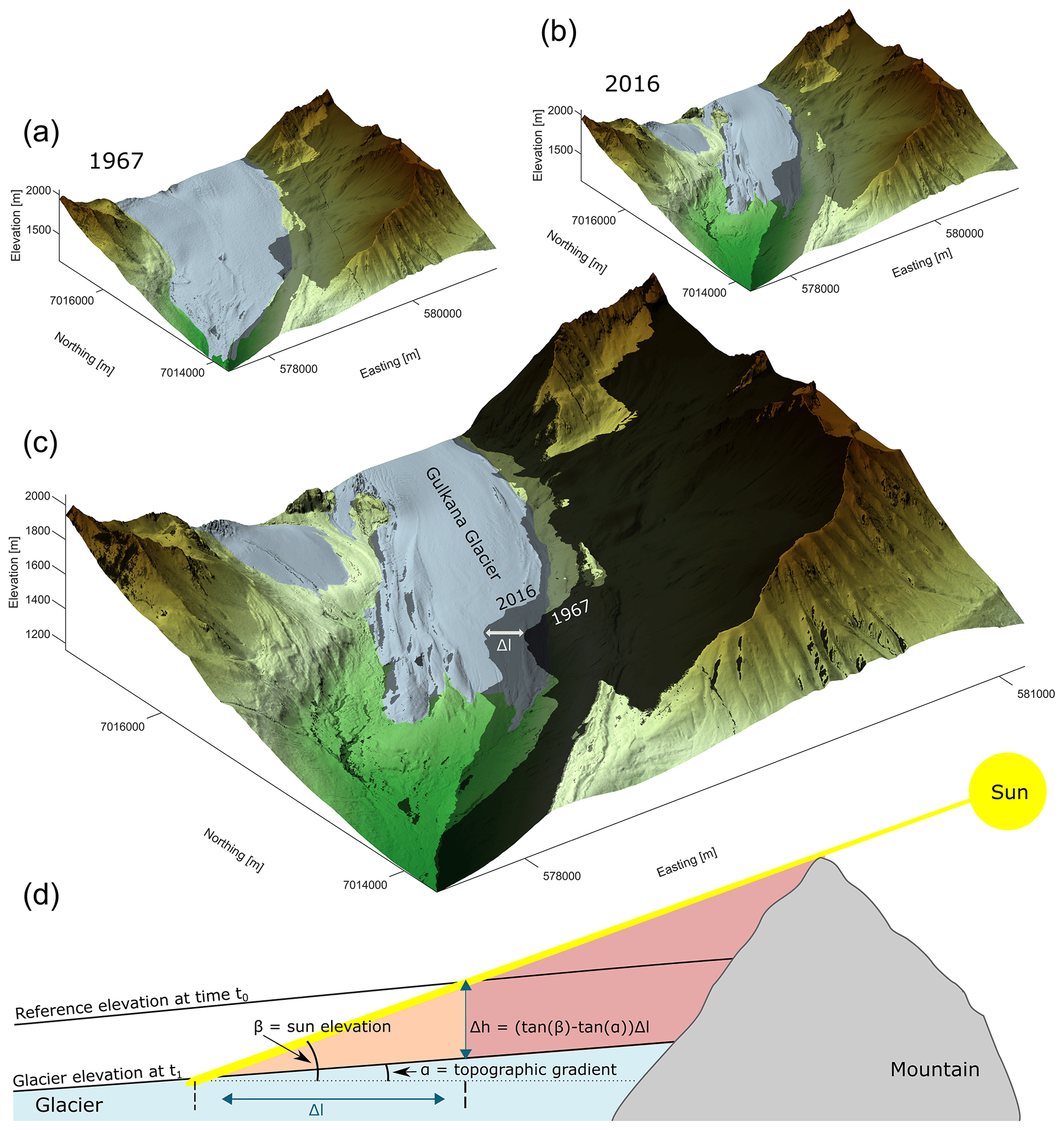
Figure 1Effects of changing glacier elevation on the length of cast shadows. Example of modelled shadows on Gulkana Glacier, Alaska, using digital elevation models and mapped glacier outlines in 2 distinct years from McNeil et al. (2022). (a) DEM and surface area (light blue) of Gulkana Glacier in 1967. (b) DEM and surface area of Gulkana Glacier in 2018. (c) DEM from 2018 with shadows from 1967 and 2018. Shadows were calculated based on a sun elevation of 20∘ and sun azimuth of 135∘. The horizontal difference between the shadows (arrow in c) is 210 m. (d) Diagram of the trigonometric relationship that predicts longer horizontal shadows under a constant sun elevation β and mountain topography, assuming that the glacier maintains its topographic gradient α. In the example, the gain in shadow length at the terminus of Gulkana Glacier translates into a glacier elevation change of ca. −76 m.
Few studies have explored the potential of cast shadows in satellite images to detect surface changes of glaciers. A recent study, for example, assessed ice-shelf freeboard heights of the Abbot Ice Shelf, Antarctica (Rada Giacaman, 2022). Another appraisal assessed the potential of the method for Great Aletsch Glacier using Sentinel-2 for the period 2017–2021 (Dematteis et al., 2023). Yet, the potential of cast shadows in glacier geodetic surveys has remained unaddressed for a broader geographic range and over longer timescales. Here we address the question of how well, if at all, we can measure elevation changes on glaciers based on the variability in shadows cast by surrounding mountains. To this end, we develop and test an approach that applies trigonometry to time series of shadows extracted from Landsat satellite images from 1986 to 2021, draped over local DEMs, in order to identify local glacier surface changes. We validate this method at five glaciers for which we have detailed information on local glacier elevation changes.
We selected glaciers in North America, Europe, and Central Asia, spanning 20∘ of latitude in the Northern Hemisphere (Fig. 2). Our selection was guided by the availability of decadal time series of glacier mass balances and high-resolution DEMs, as well as glacier outlines, providing a validation of our analysis. The shadows cast on these glaciers account for varying sun angles and surrounding relief, and they occur in accumulation as well as ablation areas.
Great Aletsch Glacier is located in the Swiss Alps, offering one of the longest consecutive records of mass balances in this mountain region (Bauder et al., 2007). The summit of Dreieckhorn casts a pronounced shadow on the Great Aletsch firn at ∼2950 m a.s.l., which is close to the estimated equilibrium line altitude (ELA) of 2961 m during the period of 1971–1990 (Zemp et al., 2007). High and steep mountains surround Baltoro Glacier in Pakistan. Mitre Peak creates a nearly triangular shadow near Concordia (∼4500 m a.s.l.), which is the confluence of Baltoro and Godwin-Austen glaciers. This shadow is likely in the ablation zone, given an ELA at ∼5200 m a.s.l. (Minora et al., 2015). The northernmost glacier in our study is Gulkana Glacier (Alaska, USA), shaded by Ogive Mountain at ∼1850 m a.s.l. in the west and by Icefall Peak at ∼1800 m a.s.l. in the east. We did not study the shadow near the tongue of Gulkana Glacier, given that most Landsat images are acquired around solar local noon when shadows are absent or very small. The ELA of Gulkana Glacier ranged from 1811 to 2178 m a.s.l. between 2009 and 2019 (McNeil et al., 2022), so the shadows were largely in the ablation zone. At South Cascade Glacier (Washington, USA), Lizard Mountain has two peaks, which form one coherent shadow on the glacier (∼2050 m a.s.l.). This shadow is above the ELA, which ranges between 1794 and 2042 m a.s.l. (1986 to 2018) (McNeil et al., 2022). Finally, Sperry Glacier (Montana, USA) is shaded at an altitude of ∼2350 m a.s.l. by Gunsight Mountain. The shadow is situated largely in the ablation zone, given an average ELA at ∼2500 m a.s.l. for the period 2005–2019 (McNeil et al., 2022).
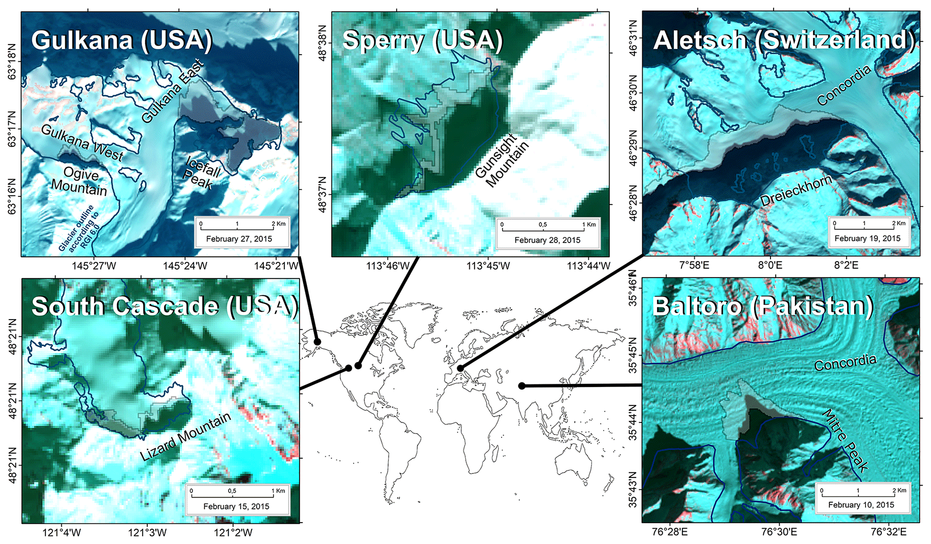
Figure 2Maps of the five study regions. Images are false-colour composites (shortwave infrared (SWIR), blue, and green bands) from Landsat OLI obtained in February 2015. Blue outlines are glaciers in the Randolph Glacier Inventory (RGI), V6.0. The semi-transparent areas show the difference between the largest and smallest shadow mapped in Landsat images in our study period, which we use for comparison with independent data and studies.
3.1 Satellite images and DEMs
We obtained 30 m resolution Landsat images (Level 1 Precision and Terrain Correction, L1TP) to map shadows on the glacier surface. To this end, we downloaded 69 cloud-free Landsat images (45 from TM, two from ETM+, and 22 from OLI) with an acquisition period between 1986 and 2021 from the USGS EarthExplorer (https://earthexplorer.usgs.gov/, last access: 18 July 2023, Supplement Table S1). L1TP images offer high radiometric and geodetic accuracy by using ground control points and correcting for topographic displacement using regional DEMs (https://www.usgs.gov/landsat-missions/landsat-levels-processing#L1TP, last access: 18 July 2023). We could not find any notable offsets between successive images in the time series.
We used several DEMs to simulate cast shadows for the dates on which the Landsat images were acquired (Table S2). For four glaciers, we used the DEM of the Shuttle Radar Topography Mission (SRTM-1, 1 arcsec spatial resolution), which corresponds to a spatial resolution of 30 m in the local projection (Farr et al., 2007). Gulkana Glacier is located beyond the maximum acquisition range of SRTM at 60∘ N. We therefore used a 2 m stereo-photogrammetric DEM of WorldView-1 data acquired in 2009, which is also part of ArcticDEM (Porter et al., 2022). Owing to high vertical uncertainties in SRTM data for rough topography (Mukul et al., 2017; Liu et al., 2019), we used additional DEMs to enhance and validate our results. For Great Aletsch Glacier, we obtained the swissALTI3D DEM (acquisition year 2017–2018, version 2019, downsampled to 5 m spatial resolution by merging multiple raster datasets). For Baltoro Glacier, we replaced Mitre Peak (the source of the shadow cast on the glacier) in the SRTM-1 DEM using data from the Viewfinder Panoramas (VFP) project (De Ferranti, 2015). VFP is an improved version of the SRTM DEM drawing on auxiliary DEMs at locations where SRTM features voids or artefacts due to phase-unwrapping errors. In the higher Himalayas, the accuracy of the SRTM DEM decreases as elevation and steepness increase (Mukul et al., 2017; Liu et al., 2019). Indeed, the original SRTM-3 DEM (3 arcsec or approximately 90 m) features a void at Mitre Peak, suggesting that its elevation was interpolated (EROS, 2018). We therefore filled this void using the VFP DEM while maintaining the elevation of the glacier from the original SRTM DEM. We also compared this modified shape of Mitre Peak against the original SRTM and other freely available DEMs (see Sect. 3.5).
3.2 Workflow for estimating trends in glacier elevation change in shaded areas
We created a binary mask of shaded and non-shaded areas (Fig. 3a) by applying a user-defined threshold to the digital numbers of the green band (encompassing a wavelength of 525–600 nm) of each Landsat scene (Supplement Table S1). We found the green band useful because shadows appear to be dark on the otherwise bright glacier surface. Snow, firn, and ice have minimal absorption in the blue–green range, whereas red and infrared light is strongly absorbed on these surfaces. This trait enhances contrast at the interface between glaciated surfaces and shaded colder areas with increasing wavelength. The incoming and reflected electromagnetic wavelength in the green band is also less affected by Rayleigh scattering in the atmosphere compared to the blue band, which has a shorter wavelength. The green band therefore offers a good compromise between contrast and surface reflectance measured at the sensor and has been successfully used in mapping glacier outlines (Paul et al., 2016). For each Landsat image, we obtained the sun azimuth and sun elevation from the associated metadata file. We used these two parameters to simulate cast shadows using a ray-tracing algorithm implemented in SAGA GIS V2.3.2 (Conrad et al., 2015). This algorithm returns a binary raster classifying each pixel as either shaded or non-shaded, equivalent to our threshold-based mapping (Fig. 3b). We then calculated the difference in area between the modelled shadow and shadows derived from Landsat images. We clipped the resulting polygons to the glacier outline in the Randolph Glacier Inventory (RGI) V6.0 (Pfeffer et al., 2014) (Fig. 3c). Within these difference polygons, we obtained the change in shadow length using bearing lines at a regular horizontal spacing of 30 m (i.e. the cell size of Landsat images) in the direction of the sun azimuth (Fig. 3d–f, Supplement Table S1). These lines represent the incoming sun rays and are assumed to be parallel, given that the sun is a far-distant, point-shaped light source. Thus, the change in shadow length is considered relatively short compared to the distance between Earth and the sun. Artefacts in the bearing lines (Fig. 3e) appeared mainly because of the limited resolution of the DEM and satellite images (i.e. interrupted lines by pixel corners, shadows at the bottom edge or in ice-free areas of the glacier), so we removed them manually. Finally, we used the trigonometric relationship of the law of tangents to convert the length of each line to changes in elevation relative to the date when the DEM was acquired (Fig. 1). Earth curvature could influence the length of the simulated shadows and thus the glacier elevation changes but only in the millimetre range, and it is therefore not considered in our analysis.
We scaled the elevation changes for each glacier so that the median for the year 2000 is zero because in most cases the data are relative to the elevation values in the SRTM DEM from February 2000. The changes in glacier elevation in the other years are therefore the positive or negative deviations from the median in 2000.
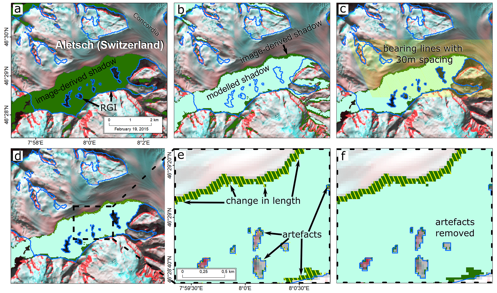
Figure 3Flowchart of modelling terrain shadows using the example of Great Aletsch Glacier. (a) Mapped shadows (green) using a digital number threshold of 5500 in a Landsat 8 image. Background image is a false-colour composite using the SWIR, blue, and green bands, and the glacier outline according to the RGI V6.0 is blue. (b) Modelled shadow (turquoise) using SAGA GIS, draped over the mapped shadow in the Landsat image. (c) Extracted shadows by RGI and parallel bearing lines from the azimuth given in the Landsat metadata. (d) Lines cut to the difference between the two shadows. (e) Close-up of (d) with generated lines of change in shadow length and unwanted artefacts. (f) Artefacts at the bottom edge and along ice-free areas removed.
We used a Bayesian multi-level linear regression model to estimate linear trends in elevation change for each glacier with time. Multi-level models can accommodate groups in data, in our case different glaciers, within a single model. We can thus estimate local effects at a given glacier with respect to the entire population learned from all data regardless of their location. Multi-level models improve parameter estimates for individual groups, in particular when differing sample sizes cause variance across the groups (McElreath, 2020). Multi-level models are suitable for datasets with different sample sizes in each group. In our case, one glacier might have hundreds of bearing lines in a given year (e.g. Great Aletsch Glacier) and others might have fewer data (e.g. Gulkana Glacier, regarding the eastern shadow). The hierarchical model structure avoids over-fitting parameters for glaciers with many bearing lines and generally improves inference for groups with few data points. The glaciers inform each other, given that groups are conditioned on the data from all glaciers, reducing uncertainty in years with few bearing lines at a given glacier. The parameters in the model are drawn from distributions specified by population-level (hyper-)parameters, which are also learned from the data. The multi-level model returns the posterior distribution for both population-level and group-level parameters.
Our likelihood function follows Student's t distribution, which is robust against outliers (Kruschke, 2014). We modelled the trend in glacier elevation change Δh with year y as
where Δh denotes the elevation changes from bearing lines in each year, i is an index for n bearing lines, and J is the number of glaciers. The likelihood function has a location parameter μ; κ is a positive scale parameter; and ν denotes the degrees of freedom, fixed at ν=3. The parameters αj and βj are the intercepts and slopes for each group, respectively, and α and β are the corresponding parameters at the population level. The covariance matrix S of the multivariate normal distribution (MVNormal) is composed of group-level standard deviations σα and σβ, and R, the correlation matrix with correlation ς. We choose the following priors to model the parameters for the entire population and all groups (i.e. the glaciers):
These priors refer to standardised data pairs (Δh and y) with zero mean and unit standard deviation. Choosing wide priors with a zero-mean Gaussian distribution and standard deviation of 2.5 admits both negative and positive trends for β, such that the posteriors are largely informed by the data. We choose a Lewandowski–Kurowicka–Joe Cholesky (LKJCholesky) correlation distribution prior for R so that all correlation matrices are equally likely. We numerically approximate this posterior using a Hamiltonian sampling algorithm implemented in Stan that is called via the software package brms within the statistical programming language R (Bürkner, 2017; R Core Team, 2022; Stan Development Team, 2022). We ran three parallel chains with 6000 iterations after 2000 warm-up runs, and we found that the Markov chains converged ( statistic =1.0). We report the posterior distributions of all model parameters in Table S3.
3.3 Comparison to reference DEMs and historical maps
We compared our estimated trends in glacier elevation change with trends from independent multi-temporal, high-resolution DEMs in shaded areas. For all glaciers in North America, we used repeated DEMs available for USGS benchmark glaciers (McNeil et al., 2022). These DEMs have spatial resolutions ranging between a few decimetres and 10 m, and they were derived from historic topographic maps, aerial stereo-photography, and spaceborne imagery. For all DEMs, we extracted the mean elevation change of all pixels between the edges of the largest and smallest mapped shadows in the Landsat images, as the shape of the shadows varies due to changing acquisition dates and sun angles. For Great Aletsch Glacier, we obtained glacier elevation changes from historical maps (Landeskarte at map scales of 1:25 000 and 1:50 000) available for 12 years between 1959 and 2020 from the Bundesamt für Landestopografie KOGIS (Koordination, Geoinformation und Services; https://www.swisstopo.admin.ch, last access: 26 March 2023). Mountain peaks in these maps are labelled with elevation values, and we consider them to have had stable terrain in the past 60 years. A sample of 10 peaks suggests positive and negative offsets of less than 5 m compared to the high-resolution swissALTI3D DEM, making these maps suitable for validating our method over a period of more than 6 decades (Fig. S1, Table S5). To infer elevation changes from contour lines in historical maps, we manually chose four points with a spacing of 1 km along a straight line in the flow direction of the glacier within the area covered by the shaded glacier (Fig. S1). For each map, we then extracted the glacier elevation at each point using linear interpolation and calculated the average elevation change from these points. We could not find any historical elevation data for Baltoro Glacier that would be suitable for comparison.
We used the same multi-level structure as above (Eqs. 1–11) to determine the trends in glacier elevation change from glaciers with repeat, high-resolution DEMs. To this end, we conditioned the model on J=5 glacier shadows (excluding Baltoro), chose the same priors, and maintained the setup of the Hamiltonian sampler. We trained two models, one with all available data and one with data limited to the Landsat period, to make trends comparable to our study period. In both cases, we found that all chains converged (), and we report all model parameters in Table S4.
3.4 Comparison to glacier elevation changes from Hugonnet et al. (2021)
In addition, we compared the elevation changes of our six study glaciers with time series from Hugonnet et al. (2021). In their study, the entire archive of satellite images from the Advanced Spaceborne Thermal Emission and Reflection Radiometer (ASTER) mission was automatically assembled into DEMs, stacked, and co-registered with other DEMs from the ArcticDEM at a spatial resolution of 100 m×100 m. In general, each pixel is covered by several dozen DEMs over the period 2000 to 2019. Noise and artefacts in the DEMs that would lead to excessively strong rates of glacier elevation change are iteratively filtered from the time series by several fixed thresholds and deviations from the reference TanDEM-X DEM, as well as by a Gaussian process (GP) regression model. Unlike our linear regression model, the GP regression model allows for seasonal, periodic oscillations in glacier elevation, so the interpolated time series of glacier elevations show seasonal variations. We used time series of glacier elevation change extracted from the area between the largest and the smallest shadow (Fig. 2), provided as summary statistics on mean glacier elevation change between 2000 and 2019 by Romain Hugonnet (personal communication, 2023) (Fig. 6). For comparison, we shortened our study period to 2000–2019 and fit the Bayesian hierarchical model with the same structure and parameterisation as above.
3.5 Sensitivity of cast shadows against globally available DEMs
The choice of the DEM may bias our estimates of glacier elevation changes because the DEMs can have different spatial resolutions, artefacts, and horizontal and vertical errors, e.g. due to foreshortening, layover, and shadow effects in radar data. These uncertainties propagate into modelled cast shadows and likely change the inference on glacier elevation change derived from different globally available DEMs (Table S2). Using Great Aletsch Glacier and Baltoro Glacier, we quantitatively and qualitatively assessed the impact of the underlying DEM on the modelled shadows.
Great Aletsch Glacier provides seven freely available DEMs. From OpenTopography (https://opentopography.org/, last access: 18 July 2023), we obtained two SRTM DEMs (SRTM-1 with 30 m and SRTM-3 with 90 m spatial resolution), NASADEM (a reanalysis of SRTM data with 30 m resolution), ALOS World 3D (AW3D30 with 30 m), and two Copernicus DEMs (GLO-30 with 30 m and GLO-90 with 90 m). We compared the DEM-derived shadows to those from the lidar-based swissALTI3D DEM, which we treat as the benchmark. In each simulation, we use a sun azimuth of 135∘ and sun elevation of 25∘ to determine how much the modelled shadow varies in shape and extent as a function of the input DEM. Accordingly, more recent DEMs should generate longer shadows if the glacier has gradually thinned during that period. We also studied the role of the DEM resolution in Landsat-derived shadows at Great Aletsch Glacier. In theory, choosing a DEM resolution coarser than Landsat (30 m) could increase the noise in the bearing lines, as one DEM pixel would cover several Landsat pixels and thus several bearing lines. To test this idea, we calculated the difference between the shadow mapped from Landsat images and the shadow simulated from three input DEMs. We then compared the variance of elevation change with time using bearing lines drawn through the swissALTI3D DEM (5 m, highest resolution), SRTM-1 (30 m, medium resolution, corresponding to that of the Landsat images), and the GLO-90 DEM (90 m, lowest resolution).
The example of Baltoro Glacier addresses the impact of the unknown elevation of Mitre Peak on the size and shape of the cast shadow. The SRTM data have gaps, so the peak is not well represented by the data, and the High Mountain Asia 8 m DEM (Shean, 2017) has wide data gaps on the west-facing slopes of Mitre Peak. Therefore, we took the void-filled SRTM-1 and SRTM-3 products as a basis; cut out Mitre Peak from these DEMs; and inserted the raster values from AW3D30, NASADEM, GLO-30, GLO-90, and VFP for the peak. We then mapped the shadow from a Landsat image obtained in February 2000 (the acquisition period of SRTM), and compared its shape against a modelled shadow using these modified input DEMs and the azimuth and elevation angle from the Landsat image. We assume that the DEM with the smallest differences between modelled and mapped shadows is most suitable for representing mountain peaks and thus elevation changes.
4.1 Glacier elevation changes from cast shadows
In each Landsat scene, between 20–110 bearing lines (2.5 %–97.5 % of the distribution; median is 31) with a regular spacing of 30 m pass through the mapped shadows on the five selected glaciers (Supplement Table S1). Individual bearing lines suggest the lowest variance in glacier elevation change at Sperry Glacier (−22 to +5 m; 2.5 % and 97.5 % of the distribution) and the highest variance at Gulkana West (−94 to +30 m), when adjusting elevation changes relative to the year 2000. Our analysis of trends in glacier elevation changes suggests that Gulkana West and Great Aletsch Glacier had the highest annual rates of thinning of and m yr−1, respectively (mean and 95 % highest density interval, HDI). The mean elevation change in the western, lower-lying branch of Gulkana Glacier is about 10 times more negative than that of the eastern, higher-lying branch. Shaded surfaces on Sperry and South Cascade glaciers have lost on average about 0.4 m yr−1 since the late 1980s. The eastern arm of Gulkana Glacier has been thinning at a credible negative, albeit low, annual rate, while the surface of Baltoro Glacier has shown no change in recent years (Fig. 4).
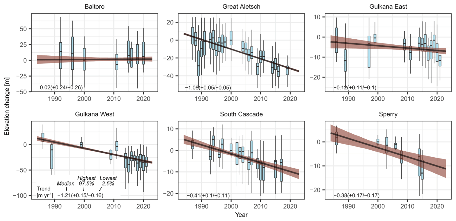
Figure 4Trends in mean elevation change on shaded glacier surfaces. Boxplots show annual glacier elevation changes, which we have derived from bearing lines drawn through shadows in Landsat images. Values of elevation change are relative to the median value in 2000 (for Gulkana Glacier in 1999). Boxes encompass the interquartile range, whiskers are 1.5 times the interquartile range, and horizontal lines are the median. Outliers (lowest and highest percent in the distribution) are removed. The thick black line is the mean posterior trend, and brown shading is the 95 % highest density interval (HDI). Numbers in the lower-left corner summarise the posterior distribution of the trend in glacier elevation change, including the median, the lower 2.5 %, and the upper 97.5 % of the HDI.
4.2 Comparison with reference DEMs
Our estimated trends from bearing lines match the trends obtained from high-resolution DEMs and historical maps (Fig. 5). However, uncertainties in the trends calculated from the reference DEMs are consistently higher given that fewer data enter the hierarchical regression model, especially if we fit the model only to data from DEMs obtained during the shorter Landsat period. At Great Aletsch Glacier, we find similar trends in mean glacier elevation change between our method ( m yr−1) and the reference DEMs, regardless if we evaluate all available DEMs dating back to 1959 ( m yr−1) or only those DEMs obtained during the shorter Landsat period () (Fig. 5). At South Cascade Glacier, the mean trend from the high-resolution DEMs is more than twice that of the trends obtained from bearing lines ( vs. m yr−1). Trends are more consistent, however, if we consider all available data from South Cascade Glacier, extending back to the late 1950s (Fig. 5). For the two shadows at Gulkana Glacier, the mean trends from the DEMs during the Landsat period are negative and midway between the very high and low values that we had determined for the two arms. Trends in historical DEMs are difficult to determine at Sperry Glacier because only two observations inform the multi-level model during the Landsat period.
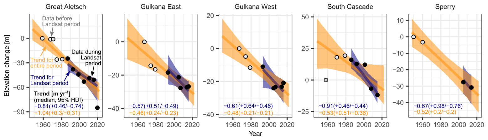
Figure 5Reported glacier elevation changes in five areas of shadow on four glaciers derived from reference DEMs. All values are relative to the first observation for each glacier, which is set to zero. Black bubbles are observations when Landsat images are available at a given glacier (see trends in Fig. 4). Grey bubbles mark data obtained before the Landsat period. Shades, thick lines, and numbers refer to models that are fit to all data from the entire period (orange) and to data for the Landsat period only (blue). Numbers in the left-lower corner summarise the posterior distribution of the annual trend in glacier elevation change, including the median, the lower 2.5 %, and the upper 97.5 % of the HDI.
4.3 Comparison with data from Hugonnet et al. (2021)
If we reduce our study period to 2000–2019, we find that our trends generally follow those of Hugonnet et al. (2021) (Fig. 6). The exception is Gulkana East, where our estimated mean rate of glacier elevation change is twice as high. The most negative trends in both methods occurred at Great Aletsch Glacier. With the exception of 1 year on Great Aletsch and Gulkana East glaciers, the Gaussian process regression models of Hugonnet et al. (2021) overlap with our data (yellow interquartile ranges of the boxes in Fig. 6), indicating good agreement between the two methods. One reason for some of the discrepancy between the two datasets may be the rigorous filtering of outliers in the dataset of Hugonnet et al. (2021), whereas our method maintains the elevation changes of all bearing lines, regardless of their distances from the mean or median.
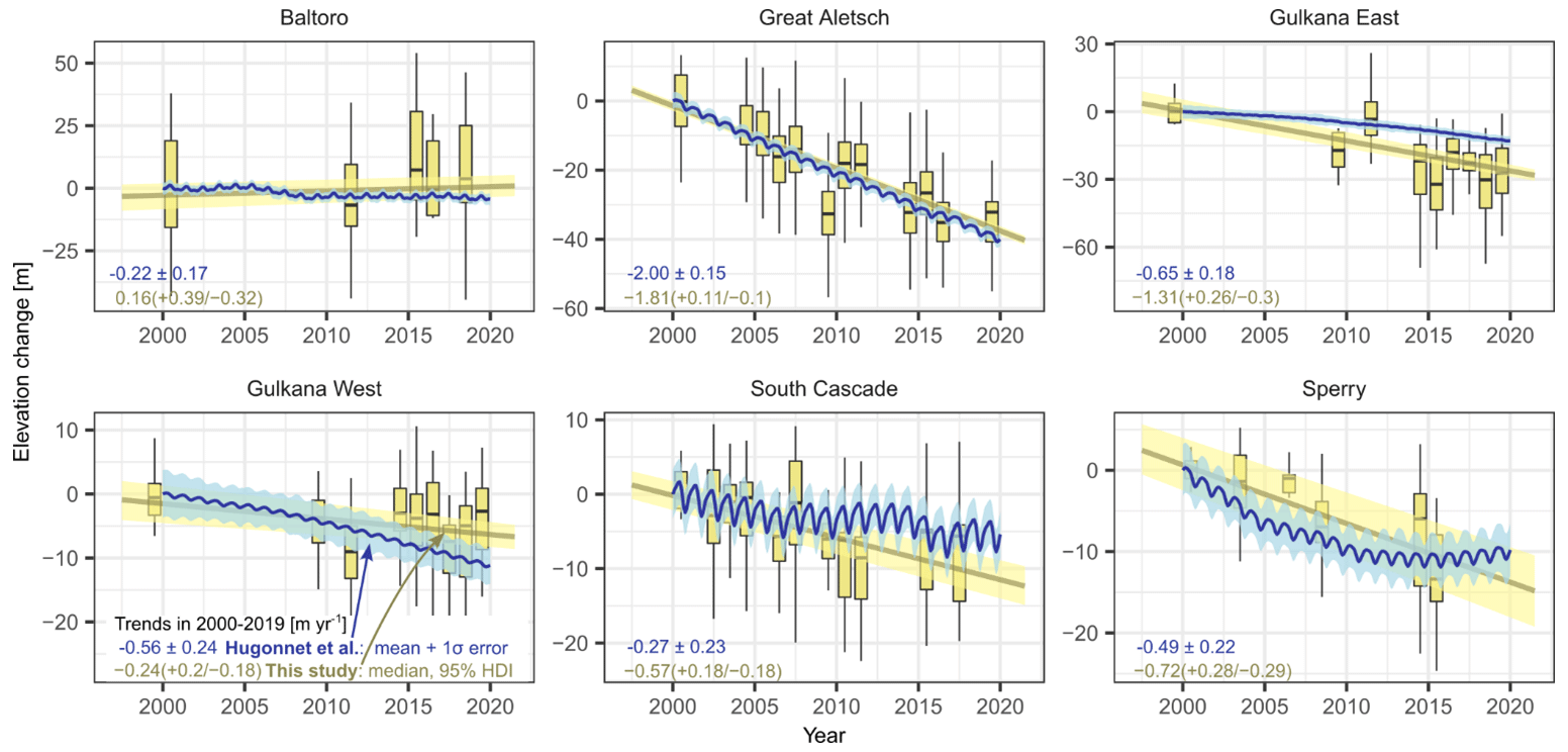
Figure 6Glacier elevation changes in shaded areas using our method and that of Hugonnet et al. (2021) for data between 2000 and 2019. All values are relative to the year 2000, which is set to zero. Yellow colours refer to our method, and blue colours are trends of glacier elevation change using Gaussian process (GP) regression through time series of ASTER DEMs from Hugonnet et al. (2021). Boxes encompass the interquartile range, whiskers are 1.5 times the interquartile range, and horizontal lines are the median. Outliers (lowest and highest percent in the distribution) are removed. The thick yellow line is the median posterior trend, and light-yellow shading is the 95 % highest density interval (HDI). Yellow numbers in the lower-left corner are our posterior estimate of the annual trend in glacier elevation change, including the mean, the lower 2.5 %, and the upper 97.5 % of the HDI. Blue numbers are the mean annual trend and 1σ error from Hugonnet et al. (2021).
4.4 Influence of DEM type and resolution
We conducted the shadow-based detection of glacier elevation changes with three DEMs for Great Aletsch Glacier (Fig. 7). The lengths of bearing lines between shadows (and derived elevation changes) vary substantially, but the shapes of nonparametric regression curves are consistent between the different DEMs. Apart from these trends, residuals from these trends are affected by the underlying DEM. Residuals of SRTM-1 and GLO-90 had a high standard deviation of 18.2 and 26.8 m. Residuals are lowest for the swissALTI3D DEM at a standard deviation of 14.3 m, suggesting that an increase in DEM resolution may improve the precision of our method.
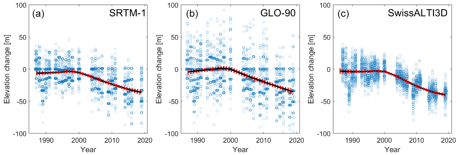
Figure 7Glacier elevation changes of Great Aletsch Glacier (see extent in Fig. 3) based on Landsat imagery and modelled shadows derived from three digital elevation models (DEMs). Semi-transparent blue points show the elevation change derived from the length of individual bearing lines between Landsat-derived shadows and those modelled from (a) the 30 m SRTM-1 DEM, (b) the 90 m GLO-90 DEM, and (c) the 5 m swissALTI3D DEM. Black lines are the means from a LOWESS (locally weighted scatterplot smoothing) regression of elevation change against time. Dashed red lines are bootstrapped confidence intervals (±2σ).
4.5 Comparison of shadows derived from DEMs
The elevation changes obtained from bearing lines have substantial variance in a given year (Fig. 4), despite covering a small range in elevation along the glacier. We infer that DEM resolution and quality have important controls on estimated glacier elevation changes from cast shadows. Indeed, the example of Great Aletsch Glacier shows that different DEMs produce shadows of different lengths, even with a constant sun azimuth and elevation (Figs. 8, 9). This variation reflects limits in the DEM resolution and the representation of ridge lines. The acquisition date may also play a role, assuming that ongoing thinning might produce longer shadows in more recent DEMs. In our example, shadows projected from the swissALTI3D DEM (5 m spatial resolution, acquisition in 2017 and 2018) extend farthest to the north (Fig. 8a). The large shadow area thus likely follows both from the reported decadal glacier thinning and from a more precise representation of the ridge line and the surrounding topography (Fig. 8a). Shadows from the GLO-30 DEM (acquisition date 2011–2015, ∼30 m spatial resolution) are very similar to those derived from the swissALTI3D DEM (Figs. 8b, 9). We also find the smallest variance in shadow length for the GLO-30 DEM (Fig. 9). Shadows derived from the GLO-90 DEM (∼90 m resolution) show both a larger spatial offset (Fig. 8c) and a higher variability in shadow length (Fig. 9). We attribute this mismatch to a higher degree of spatial averaging, causing lower topographic ridges due to the coarser spatial resolution. Shadows derived from the AW3D30 DEM (acquisition period between 2006 and 2011, ∼30 m spatial resolution) are highly variable compared to the swissALTI3D DEM (Fig. 8d). Some of the shadows extend beyond those derived from the swissALTI3D DEM, an effect of exaggerated topography in the DEM that overestimates the height of the ridge (Fig. 9). Finally, shadows derived from the SRTM DEMs and NASADEM (Fig. 8e–g) – all derived from data acquired from the same shuttle mission in 2000 – show the highest difference from the swissALTI3D DEM. SRTM DEMs and NASADEM-derived shadows are very similar, but again, the coarser SRTM-3 DEM leads to a lowering of the ridges and larger horizontal distances.
The absence of high-resolution data and presence of voids in the SRTM data covering Baltoro Glacier and Mitre Peak prompted us to use the VFP DEM to obtain the shape of the steep and peaked mountain. We assume that the unknown acquisition date of topographic data in the VFP DEM has little impact on our subsequent analysis as Mitre Peak is free of glacier ice and no major rockfalls were reported during our study period that could have reduced its elevation. To evaluate this choice, we compared the modelled shadows based on elevation data of Mitre Peak obtained from all DEMs with the actual shadows cast by the mountain in 2020 (Fig. 10). The VFP DEM has a spatial resolution of 3 arcsec (90 m), which suggests that it will perform less well than the other DEMs with higher resolution. However, visual comparison shows that the VFP DEM captures the actual shadows more precisely, which is consistent with >100 m higher peak elevations than those contained in the other DEMs (Fig. 10).
In summary, variations in modelled shadows obtained from different DEMs not only relate to variable acquisition dates but also reflect how accurately ridge topography is represented in the DEMs. Comparison of DEMs with the same acquisition date but different spatial resolution shows that coarser DEMs underestimate ridge height and commensurately shadow length. Notwithstanding, a general trend towards longer shadows and thus a trend towards lower glacier elevations can be observed for younger acquisition dates (Fig. 9).
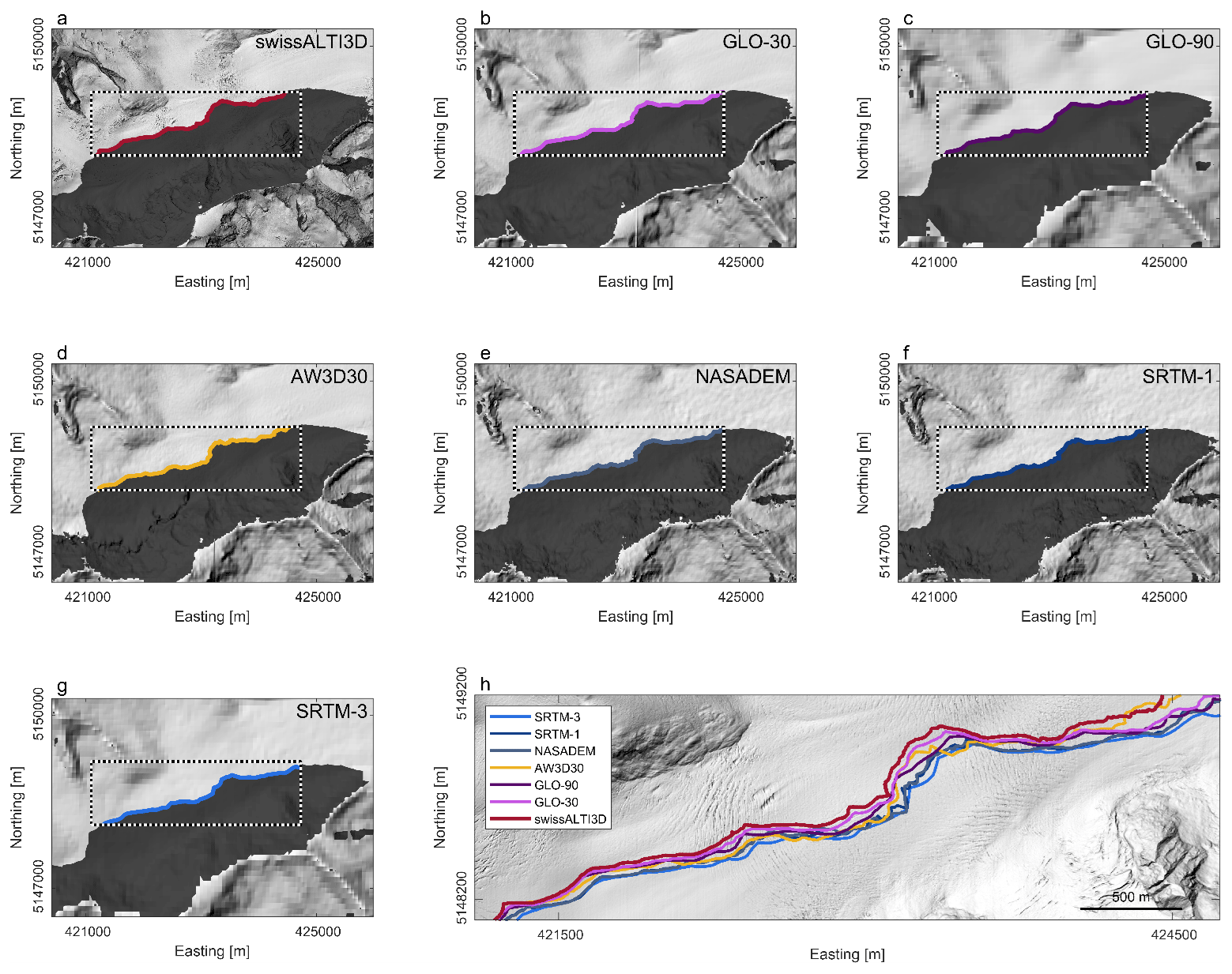
Figure 8Shadows projected onto Great Aletsch Glacier using different digital elevation models. (a–g) Grey hillshade shows the simulated cast shadow using a sun azimuth of 135∘ and elevation of 25∘. (h) Close-up of the shadow outlines modelled with different DEMs. Hillshade in the background is from the swissALTI3D DEM.
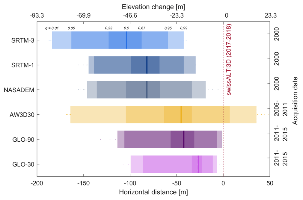
Figure 9Difference in the lengths (and corresponding elevation changes) of bearing lines crossing a shadow on Great Aletsch Glacier using six DEMs and the benchmark swissALTI3D DEM.
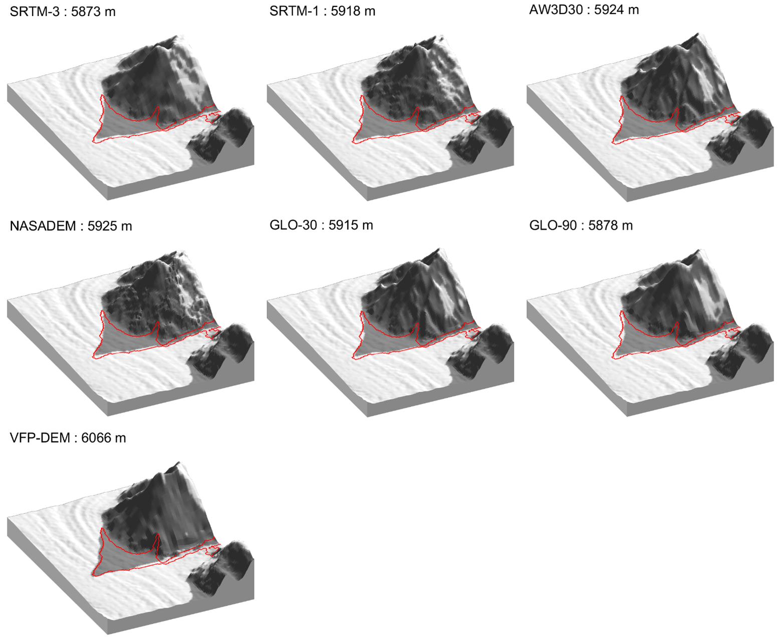
Figure 10Three-dimensional surface views including modelled and mapped shadows cast from Mitre Peak onto Baltoro Glacier, Pakistan. We used SRTM-1 and replaced Mitre Peak with elevation data from different DEMs. Shadows were calculated with an azimuth of 151.9∘ and a sun elevation angle of 29.5∘. These values refer to the sun position during the acquisition time (24 January 2000) of the Landsat image from which shadows were mapped (red outline). Visual comparison shows that the VFP-filled SRTM-1 creates the best match between modelled and actual cast shadows of the peak, whereas there are pronounced offsets between actual shadows and those derived from other DEMs. Elevation values indicate the peak altitude of Mitre Peak in each DEM.
We developed and assessed a method that measures glacier elevation changes in remote areas based on cast shadows from adjacent mountains. The precision and accuracy of the method depend on several factors that pertain to the individual processing steps and the input data (Rada Giacaman, 2022). We show that DEM quality and resolution cause variability in the detected elevation changes (Figs. 7–9). To this end, we assessed the length of bearing lines that link the shadow outlines along the azimuth direction. We find that spatial resolution affects the precision and accuracy of these lines (Fig. 7). First, DEMs with coarser resolution decrease the precision due to spatial averaging, blurring ridge topography by smoothing peaks and saddles (Purinton and Bookhagen, 2017). This effect may be more pronounced in SRTM data, which can have high errors on steep slopes and often poorly represent ridges and valley bottoms (Gorokhovich and Voustianiouk, 2006; Schwanghart and Scherler, 2017). Coarser resolution also biases or decreases the accuracy of our estimates because DEM values along ridges are lowered by spatial averaging (Fujita et al., 2008). Both effects entail that modelled shadow outlines on glaciers increasingly lack detail and underestimate shadow length with coarser DEM resolution (Fig. 9). Poor quality of the underlying DEM will propagate into our estimates of glacier elevation change although trends derived from different DEMs are surprisingly consistent (Fig. 7). Cast shadows from satellite imagery obtained for the date of DEM acquisition can help quantify and correct for such biases.
Besides differences in resolution, the type of DEM also impacts the precision and accuracy of modelled shadows. Our analysis shows that among the DEMs with global coverage, the new GLO-30 DEM has the highest precision of derived shadows when compared to the benchmark swissALTI3D DEM (Fig. 9), which is consistent with recent DEM assessments that underscore the high performance of the GLO-30 DEM (Guth and Geoffroy, 2021). Shadow outlines calculated from NASADEM and SRTM-1 are similar as they are obtained from the same data. We acknowledge that our method leaves any effects of synthetic aperture radar (SAR) penetration into the snowpack covering the glacier ice (Berthier et al., 2006) unconsidered. Yet, this offset can be treated as a constant when drawing bearing lines through shadows, given that the input DEM (SRTM) remains unchanged in our analysis. Snow cover can be thick in accumulation areas and may lead to biases (underestimates) when calculating glacier volume changes from DEM differencing (Gardelle et al., 2012). Though most shadows in our cases are in ablation zones, we recommend accounting for differing penetration depth in future studies that also include shadows on glaciers at very high elevations in snow accumulation areas. The relatively low performance of the AW3D30 DEM in comparison to other global DEMs likely relates to hillslope and ridge artefacts caused by errors in optical DEM generation (Purinton and Bookhagen, 2017). Where steep topography severely impacts DEM quality, manually edited DEMs such as the VFP DEM can provide a viable alternative despite their relatively coarse spatial resolution. In any case, our Bayesian framework objectively propagates these errors and uncertainties. One promising avenue for future research is to use more informed priors based on previous research on glacier elevation change (Hugonnet et al., 2021). Narrower and stronger priors may reduce the width of our posterior trends on glacier elevation changes that we currently observe at Sperry Glacier for example (Fig. 4). They might also offer a better compromise to balance some of the differences within our data (e.g. between Gulkana East and Gulkana West) and also between our data and data from previous research. One of these examples may be the outstanding trend at Gulkana West (Fig. 6), where the physical causes and methodological differences between our appraisals and the appraisal of Hugonnet et al. (2021) remain to be determined.
In addition to the resolution and quality of the DEM, we expect that higher image resolution will warrant a higher accuracy and precision at which elevation changes can be detected (Fig. 7). We refrained from analysing the effects of image resolution because we used only Landsat imagery, which comprises the longest freely available time series of satellite imagery. We recall that our trigonometric approach hinges on sun elevation and image resolution provided in the image metadata, both setting the detection limit of elevation changes. For example, for a sun elevation of 20∘ and a spatial resolution of 30 m, a minimum elevation change of 10.9 m can be detected, unless subpixel classification approaches or pan-sharpening techniques are adopted (Liu and Wu, 2005). The sun angle will be critical for our method (Rada Giacaman, 2022), and we expect that our approach works better for images acquired during the winter months of the respective hemispheres as well as at higher latitudes. To determine interannual trends, we recommend using satellite imagery with similar time stamps within a year, given that glacier elevations are prone to seasonal variations (Moholdt et al., 2010).
Atmospheric refraction – the bending of solar light as it traverses the atmosphere – causes an apparently higher sun elevation. The offset between the actual and apparent solar position leads to errors in shadow-height applications depending mainly on solar elevation and, to a minor degree, on atmospheric pressure, humidity, and temperature (Rada Giacaman, 2022). Sun elevations in our study range between 15 and 40∘, which yields height difference errors of 0 %–2 % (see Fig. 10 in Rada Giacaman, 2022). Additional error sources include uncertainties in the position of the satellite as well as problems in image registration and deformation. Yet, we did not account for errors due to atmospheric refraction and image registration as they appear minor compared to those related to image resolution and DEM quality.
Our study reveals and confirms decadal-scale loss of glacier mass. These changes are consistent with independent estimates of glacier elevation changes based on stereo-photogrammetric analysis of US benchmark glaciers, i.e. South Cascade, Gulkana, and Sperry glaciers (McNeil et al., 2022), and historic topographic maps of Great Aletsch Glacier (Fischer et al., 2015; Leinss and Bernhard, 2021). For Baltoro Glacier, we detect no credible trends, and independent, field-based validation data of surface changes at the shadow location are lacking. Yet, comparison of photographs from 1909 and 2004 shows that glacier elevation changes at Concordia were low in the 20th century (<40 m) (Mayer et al., 2006). These small rates of surface lowering have been attributed to increases in precipitation and a lowering of summer mean and minimum temperatures in the Karakoram, supporting regionally unchanged glacier masses referred to as the “Karakoram anomaly” (Hewitt, 2005; Kääb et al., 2015; Forsythe et al., 2017; Farinotti et al., 2020).
We stress that our results are tied to local changes in shadows cast from adjacent mountains. Thus, we caution against comparing our results directly with glacier-wide mass balances because these are integrated over entire glaciers or elevation bands within glaciers and may refer to different study periods. For example, Hugonnet et al. (2021) estimate that the entire areas of Great Aletsch and South Cascade glaciers had elevation changes of and m yr−1 (mean and 1σ error), respectively, in 2000–2019. Our estimates are less negative ( and m yr−1, respectively) in the longer Landsat period, either because we measure elevation changes at higher parts of the glacier, where the pattern of local accumulation, melt, and ice dynamics differs from that of the whole glacier, or because glacier melt has accelerated in recent years (Hugonnet et al., 2021). Indeed, if we shorten the study period to the years 2000–2019, Great Aletsch Glacier shows a trend of elevation change that is almost twice as high as that for the much longer trend going back to the 1980s. We thus envision that our method could enhance, complement, and amend geodetic surveys in ablation and accumulation areas (Beedle et al., 2014). Our method can be applied globally but is restricted to those glaciers that are surrounded by stable topography. Our method becomes unsuccessful when the shadow edge constantly falls onto bedrock due to progressive glacier retreat – a situation that will soon occur at the dwindling Sperry Glacier for example. Ideal environments for our approach are glaciers close to steep topography in high latitudes, producing cast shadows long enough to infer differences in bearing lines. Suitable sites remain to be identified and should, at best, have high-resolution DEMs with high precision and accuracy available. Locations with large landslides that lower mountain peaks (Shugar et al., 2021) should be avoided as they may violate the assumption of unaltered ridge topography over time. The processing steps developed in this study can be fully automated although quality control of the obtained bearing lines connecting modelled and actual shadow outlines are crucial.
In summary, we show that cast shadows offer avenues to retrieve glacier elevation changes from satellite imagery over many decades. We demonstrate for select cases that our method provides quantitative information about local changes in glacier elevation with time. These changes are consistent with independent DEMs of difference in shaded areas. Accurately resolving glacier elevation changes hinges on the spatial resolution of the satellite imagery from which we mapped shadows, as well as on the quality and resolution of the underlying DEM. Upon the emergence of global, void-free, high-resolution satellite images and DEMs, our method can be extended to historical satellite and aerial imagery, assuming that the geometry of mountain ridges and peaks remains unchanged with time. We conclude that our approach has the potential to complement existing or future in situ measuring networks anywhere on Earth where mountains shade parts of adjacent glaciers. We thus enrich the glaciological and geodetic toolbox with a new method that helps quantify glacier elevation changes, especially at high altitudes with limited access.
The outlines of the shadows, the bearing lines, tables with inferred elevation changes for each glacier, and the Bayesian multi-level models are available via Zenodo (https://doi.org/10.5281/zenodo.8087360, Pfau et al., 2022). Landsat images were obtained from EarthExplorer (https://earthexplorer.usgs.gov/, last access: 21 January 2023, https://doi.org/10.5066/F71835S6, Earth Resources Observation and Science (EROS) Center, 2018a, https://doi.org/10.5066/F7WH2P8G, Earth Resources Observation and Science (EROS) Center, 2018b, https://doi.org/10.5066/F7N015TQ, Earth Resources Observation and Science (EROS) Center, 2018c), and all DEMs from which we derived shadows are freely available from the sources provided in Table S2. DEMs for validation are available at https://doi.org/10.5066/P9R8BP3K (McNeil et al., 2019). Codes to fit the Bayesian multi-level models are available at GitHub (https://github.com/geveh/ShadowsOnGlaciers, last access: 21 August 2023) and Zenodo (https://doi.org/10.5281/zenodo.8269242, Veh, 2023).
The supplement related to this article is available online at: https://doi.org/10.5194/tc-17-3535-2023-supplement.
All authors contributed equally to designing the study, conducting the analysis, validating the results, and writing the manuscript.
The contact author has declared that none of the authors has any competing interests.
Publisher’s note: Copernicus Publications remains neutral with regard to jurisdictional claims in published maps and institutional affiliations.
We are indebted to the help from Romain Hugonnet, who provided data on elevation changes along shaded glacier surfaces. This work is based on global DEM services provided by the OpenTopography Facility with support from the National Science Foundation under NSF award numbers 1948997, 1948994, and 1948857.
Monika Pfau was supported for 1 year by a fellowship from the German Academic Exchange Service (DAAD) within the project Co-PREPARE, a collaboration between the University of Potsdam and the Indian Institute of Technology Roorkee. Article processing charges were covered by the Deutsche Forschungsgemeinschaft (DFG, German Research Foundation) – project no. 491466077.
This paper was edited by Etienne Berthier and reviewed by Erik Mannerfelt and one anonymous referee.
Azam, M. F., Kargel, J. S., Shea, J. M., Nepal, S., Haritashya, U. K., Srivastava, S., Maussion, F., Qazi, N., Chevallier, P., Dimri, A. P., Kulkarni, A. V., Cogley, J. G., and Bahuguna, I.: Glaciohydrology of the Himalaya-Karakoram, Science, 373, 6557, https://doi.org/10.1126/science.abf3668, 2021.
Bauder, A., Funk, M., and Huss, M.: Ice-volume changes of selected glaciers in the Swiss Alps since the end of the 19th century, Ann. Glaciol., 46, 145–149, https://doi.org/10.3189/172756407782871701, 2007.
Beedle, M. J., Menounos, B., and Wheate, R.: An evaluation of mass-balance methods applied to Castle creek Glacier, British Columbia, Canada, J. Glaciol., 60, 262–276, https://doi.org/10.3189/2014JoG13J091, 2014.
Belart, J. M. C., Magnússon, E., Berthier, E., Gunnlaugsson, Á. Þ., Pálsson, F., Aðalgeirsdóttir, G., Jóhannesson, T., Thorsteinsson, T., and Björnsson, H.: Mass Balance of 14 Icelandic Glaciers, 1945–2017: Spatial Variations and Links With Climate, Front. Earth Sci., 8, 163, https://doi.org/10.3389/feart.2020.00163, 2020.
Berthier, E., Arnaud, Y., Vincent, C., and Rémy, F.: Biases of SRTM in high-mountain areas: Implications for the monitoring of glacier volume changes, Geophys. Res. Lett., 33, L08502, https://doi.org/10.1029/2006GL025862, 2006.
Bolch, T., Pieczonka, T., and Benn, D. I.: Multi-decadal mass loss of glaciers in the Everest area (Nepal Himalaya) derived from stereo imagery, The Cryosphere, 5, 349–358, https://doi.org/10.5194/tc-5-349-2011, 2011.
Brighenti, S., Tolotti, M., Bruno, M. C., Wharton, G., Pusch, M. T., and Bertoldi, W.: Ecosystem shifts in Alpine streams under glacier retreat and rock glacier thaw: A review, Sci. Total Environ., 675, 542–559, https://doi.org/10.1016/j.scitotenv.2019.04.221, 2019.
Bürkner, P. C.: brms: An R Package for Bayesian Multilevel Models Using Stan, J. Stat. Softw., 80, 1–28, https://doi.org/10.18637/jss.v080.i01, 2017.
Cauvy-Fraunié, S. and Dangles, O.: A global synthesis of biodiversity responses to glacier retreat, Nature Ecology & Evolution, 3, 1675–1685, https://doi.org/10.1038/s41559-019-1042-8, 2019.
Conrad, O., Bechtel, B., Bock, M., Dietrich, H., Fischer, E., Gerlitz, L., Wehberg, J., Wichmann, V., and Böhner, J.: System for Automated Geoscientific Analyses (SAGA) v. 2.1.4, Geosci. Model Dev., 8, 1991–2007, https://doi.org/10.5194/gmd-8-1991-2015, 2015.
Dehecq, A., Gardner, A. S., Alexandrov, O., McMichael, S., Hugonnet, R., Shean, D., and Marty, M.: Automated Processing of Declassified KH-9 Hexagon Satellite Images for Global Elevation Change Analysis Since the 1970s, Front. Earth Sci., 8, https://doi.org/10.3389/feart.2020.566802, 2020.
De Ferranti, J.: Digital Elevation Data: SRTM Void Fill, Viewfinder Panoramas, http://www.viewfinderpanoramas.org/voidfill.html (last access: 28 August 2022), 2015.
Dematteis, N., Giordan, D., Crippa, B., and Monserrat, O.: Measuring Glacier Elevation Change by Tracking Shadows on Satellite Monoscopic Optical Images, IEEE Geosci. Remote S., 20, 1–5, https://doi.org/10.1109/LGRS.2022.3231659, 2023.
Earth Resources Observation and Science (EROS) Center: USGS EROS Archive – Landsat Archives – Landsat 8 OLI (Operational Land Imager) and TIRS (Thermal Infrared Sensor) Level-1 Data Products, Earth Resources Observation and Science (EROS) Center [data set], https://doi.org/10.5066/F71835S6, 2018a.
Earth Resources Observation and Science (EROS) Center: USGS EROS Archive – Landsat Archives – Landsat 7 Enhanced Thematic Mapper Plus (ETM+) Level-1 Data Products, Earth Resources Observation and Science (EROS) Center [data set], https://doi.org/10.5066/F7WH2P8G, 2018b.
Earth Resources Observation and Science (EROS) Center: USGS EROS Archive – Landsat Archives – Landsat 4-5 Thematic Mapper (TM) Level-1 Data Products, Earth Resources Observation and Science (EROS) Center [data set], https://doi.org/10.5066/F7N015TQ. 2018c.
EROS (Earth Resources Observation And Science) Center: USGS EROS Archive – Digital Elevation – Shuttle Radar Topography Mission (SRTM) Non-Void Filled, https://www.usgs.gov/centers/eros/science/usgs-eros-archive-digital-elevation-shuttle-radar-topography-mission-srtm-non (last access: 28 March 2023), 2018.
Farías-Barahona, D., Sommer, C., Sauter, T., Bannister, D., Seehaus, T. C., Malz, P., Casassa, G., Mayewski, P. A., Turton, J. V., and Braun, M. H.: Detailed quantification of glacier elevation and mass changes in South Georgie, Environ. Res. Lett., 15, 34036, https://doi.org/10.1088/1748-9326/ab6b32, 2020.
Farinotti, D., Huss, M., Fürst, J. J., Landmann, J., Machguth, H., Maussion, F., and Pandit, A.: A consensus estimate for the ice thickness distribution of all glaciers on Earth, Nat. Geosci., 12, 168–173, https://doi.org/10.1038/s41561-019-0300-3, 2019.
Farinotti, D., Immerzeel, W. W., De Kok, R., Quincey, D. J., and Dehecq, A.: Manifestations and mechanisms of the Karakoram glacier Anomaly, Nat. Geosci., 13, 8–16, https://doi.org/10.1038/s41561-019-0513-5, 2020.
Farr, T. G., Rosen, P. A., Caro, E., Crippen, R., Duren, R., Hensley, S., Kobrick, M., Paller, M., Rodriguez, E., Roth, L., Seal, D., Shaffer, S., Shimada, J., Umland, J., Werner, M., Oskin, M., Burbank, D., and Alsdorf, D.: The Shuttle Radar Topography Mission, Rev. Geophys., 45, 2005RG000183, https://doi.org/10.1029/2005RG000183, 2007.
Fischer, M., Huss, M., and Hoelzle, M.: Surface elevation and mass changes of all Swiss glaciers 1980–2010, The Cryosphere, 9, 525–540, https://doi.org/10.5194/tc-9-525-2015, 2015.
Forsythe, N., Fowler, H. J., Li, X. F., Blenkinsop, S., and Pritchard, D.: Karakoram temperature and glacial melt driven by regional atmospheric circulation variability, Nat. Clim. Change, 7, 664–670, https://doi.org/10.1038/nclimate3361, 2017.
Fujita, K., Suzuki, R., Nuimura, T., and Sakai, A.: Performance of ASTER and SRTM DEMs, and their potential for assessing glacial lakes in the Lunana region, Bhutan Himalaya, J. Glaciol., 54, 220–228, https://doi.org/10.3189/002214308784886162, 2008.
Gardelle, J., Berthier, E., and Arnaud, Y.: Impact of resolution and radar penetration on glacier elevation changes computed from DEM differencing, J. Glaciol., 58, 419–422, https://doi.org/10.3189/2012JoG11J175, 2012.
Geyman, E. C., van Pelt, W. J. J., Maloof, A. C., Aas, H. F., and Kohler, J.: Historical glacier change on Svalbard predicts doubling of mass loss by 2100, Nature, 601, 374–379, https://doi.org/10.1038/s41586-021-04314-4, 2022.
Gorokhovich, Y. and Voustianiouk, A.: Accuracy assessment of the processed SRTM-based elevation data by CGIAR using field data from USA and Thailand and its relation to the terrain characteristics, Remote Sens. Environ., 104, 409–415, https://doi.org/10.1016/j.rse.2006.05.012, 2006.
Guth, P. L. and Geoffroy, T. M.: LiDAR point cloud and ICESat-2 evaluation of 1 second global digital elevation models: Copernicus wins, T. GIS, 25, 2245–2261, https://doi.org/10.1111/tgis.12825, 2021.
Hewitt, K.: The Karakoram Anomaly? Glacier Expansion and the “Elevation Effect”, Karakoram Himalaya, Mountain Research and Development, 25, 332–340, https://doi.org/10.1659/0276-4741(2005)025[0332:TKAGEA]2.0.CO;2, 2005.
Huggel, C., Clague, J. J., and Korup, O.: Is climate change responsible for changing landslide activity in high mountains?, Earth Surf. Proc. Land., 37, 77–91, https://doi.org/10.1002/esp.2223, 2012.
Hugonnet, R., McNabb, R., Berthier, E., Menounos, B., Nuth, C., Girod, L., Farinotti, D., Huss, M., Dussaillant, I., Brun, F., and Kääb, A.: Accelerated global glacier mass loss in the early twenty-first century, Nature, 592, 726–731, https://doi.org/10.1038/s41586-021-03436-z, 2021.
IPCC: Special Report on the Ocean and Cryosphere in a Changing Climate, edited by: Pörtner, H.-O., Roberts, D. C., Masson-Delmotte, V., Zhai, P., Tignor, M., Poloczanska, E., Mintenbeck, K., Alegría, A., Nicolai, M., Okem, A., Petzold, J., Rama, B., and Weyer, N. M., https://www.ipcc.ch/srocc/ (last access: 28 August 2022), 2019.
Kääb, A., Treichler, D., Nuth, C., and Berthier, E.: Brief Communication: Contending estimates of 2003–2008 glacier mass balance over the Pamir–Karakoram–Himalaya, The Cryosphere, 9, 557–564, https://doi.org/10.5194/tc-9-557-2015, 2015.
Kääb, A., Winsvold, S., Altena, B., Nuth, C., Nagler, T., and Wuite, J.: Glacier Remote Sensing Using Sentinel-2. Part I: Radiometric and Geometric Performance, and Application to Ice Velocity, Remote Sensing, 8, 598, https://doi.org/10.3390/rs8070598, 2016.
Kruschke, J.: Doing Bayesian data analysis. A tutorial with R, JAGS, and Stan, 2nd ed., Elsevier, ISBN 978-0-12-405888-0, 2014.
Leinss, S. and Bernhard, P.: TanDEM-X:Deriving InSAR Height Changes and Velocity Dynamics of Great Aletsch Glacier, IEEE J. Sel. Top. Appl., 14, 4798–4815, https://doi.org/10.1109/JSTARS.2021.3078084, 2021.
Li, D., Lu, X., Overeem, I., Walling, D. E., Syvitski, J., Kettner, A. J., Bookhagen, B., Zhou, Y., and Zhang, T.: Exceptional increases in fluvial sediment fluxes in a warmer and wetter High Mountain Asia, Science, 374, 599–603, https://doi.org/10.1126/science.abi9649, 2021.
Li, H., Xu, L., Shen, H., and Zhang, L.: A general variational framework considering cast shadows for the topographic correction of remote sensing imagery, ISPRS J. Photogramm., 117, 161–171, https://doi.org/10.1016/j.isprsjprs.2016.03.021, 2016.
Liu, K., Song, C., Ke, L., Jiang, L., Pan, Y., and Ma, R.: Global open-access DEM performances in Earth's most rugged region High Mountain Asia: A multi-level assessment, Geomorphology 338, 16–26, https://doi.org/10.1016/j.geomorph.2019.04.012, 2019.
Liu, W. and Wu, E. Y.: Comparison of non-linear mixture models: sub-pixel classification, Remote Sens. Environ., 94, 145–154, https://doi.org/10.1016/j.rse.2004.09.004, 2005.
Lovell, A. M., Carr, J. R., and Stokes, C. R.: Topographic controls on the surging behaviour of Sabche Glacier, Nepal (1967 to 2017), Remote Sensing of Environment, 210, 434–443, https://doi.org/10.1016/j.rse.2018.03.036, 2018.
Mannerfelt, E. S., Dehecq, A., Hugonnet, R., Hodel, E., Huss, M., Bauder, A., and Farinotti, D.: Halving of Swiss glacier volume since 1931 observed from terrestrial image photogrammetry, The Cryosphere, 16, 3249–3268, https://doi.org/10.5194/tc-16-3249-2022, 2022.
Mayer, C., Lambrecht, A., Belò, M., Smiraglia, C., and Diolaiuti, G.: Glaciological characteristics of the ablation zone of Baltoro glacier, Karakoram, Pakistan, Ann. Glaciol., 43, 123–131, https://doi.org/10.3189/172756406781812087, 2006.
McElreath, R.: Statistical Rethinking, Chapman and Hall/CRC, 2nd Edn., ISBN 978-0-367-13991-9, 2020.
McNeil, C. J., Florentine, C. E., Bright, V. A. L., Fahey, M. J., McCann, E., Larsen, C. F., Thomas, E. E., Shean, D. E., McKeon, L. A., March, R. S., Keller, W., Whorton, E. N., O'Neel, S., Baker, E. H., Sass, L. C., and Bollen, K. E.: Geodetic Data for USGS Benchmark Glaciers: Orthophotos, Digital Elevation Models, Glacier Boundaries and Surveyed Positions, version 2.0, US Geological Survey data release [data set], https://doi.org/10.5066/P9R8BP3K, 2022.
Millan, R., Mouginot, J., Rabatel, A., and Morlighem, M.: Ice velocity and thickness of the world's glaciers, Nat. Geosci., 15, 124–129, https://doi.org/10.1038/s41561-021-00885-z, 2022.
Milner, A. M., Khamis, K., Battin, T. J., Brittain, J. E., Barrand, N. E., Füreder, L., Cauvy-Fraunié, S., Gíslason. G. M., Jacobsen, D., Hannah, D. M., Hodson, A. J., Hood, E., Lencioni, V., Ólafsson, J. S., Robinson, C. T., Traner, M., and Brown, L. E.: Glacier shrinkage driving global changes in downstream systems, P. Natl. Acad. Sci. USA, 114, 9770–9778, https://doi.org/10.1073/pnas.1619807114, 2017.
Minora, U., Senese, A., Bocchiola, D., Soncini, A., D'agata, C., Ambrosini, R., Mayer, C., Lambrecht, A., Vuillermoz, E., Smiraglia, C., and Diolaitui, G.: A simple model to evaluate ice melt over the ablation area of glaciers in the Central Karakoram National Park, Pakistan, Ann. Glaciol., 56, 202–216, https://doi.org/10.3189/2015AoG70A206, 2015.
Moholdt, G., Nuth, C. Hagen, J. O., and Kohler, J.: Recent elevation changes of Svalbard glaciers derived from ICESat laser altimetry, Remote Sens. Environ., 114, 2756–2767, https://doi.org/10.1016/j.rse.2010.06.008, 2010.
Mukul, M., Srivastava, V., Jade, S., and Mukul, M.: Uncertainties in the Shuttle Radar Topography Mission (SRTM) Heights: Insights from the Indian Himalaya and Peninsula, Sci. Rep., 7, 41672, https://doi.org/10.1038/srep41672, 2017.
Neckel, N., Kropáček, J., Bolch, T., and Hochschild, V.: Glacier mass changes on the Tibetan Plateau 2003–2009 derived from ICESat laser altimetry measurements, Environ. Res. Lett., 9, 14009, https://doi.org/10.1088/1748-9326/9/1/014009, 2014.
Paul, F., Andreassen, L. M., and Winsvold, S. H.: A new glacier inventory for the Jostedalsbreen region, Norway, from Landsat TM scenes of 2006 and changes since 1966, Ann. Glaciol., 52, 153–162, https://doi.org/10.3189/172756411799096169, 2011.
Paul, F., Kääb, A., Maisch, M., Kellenberger, T., and Haeberli, W.: International Glaciological Society: The new remote-sensing-derived Swiss glacier inventory: I. Methods, Ann. Glaciol., 34, 355–361, 2002.
Paul, F., Winsvold, S., Kääb, A., Nagler, T., and Schwaizer, G.: Glacier Remote Sensing Using Sentinel-2. Part II: Mapping Glacier Extents and Surface Facies, and Comparison to Landsat 8, Remote Sensing, 8, 575, https://doi.org/10.3390/rs8070575, 2016.
Pfau, M., Veh, G., and Schwanghart, W.: Data for “Cast shadows reveal changes in glacier surface elevation” (Version 3), Zenodo [data set], https://doi.org/10.5281/zenodo.8087360, 2022.
Pfeffer, W. T., Arendt, A. A., Bliss, A., Bolch, T., Cogley, J. G., Gardner, A. S., Hagen, J. O., Hock, R., Kaser, G., Kienholz, C., Miles, E. S., Moholdt, G., Mölg, N., Paul, F., Radić, V., Rastner, P., Raup, B. H., Rich, J., Sharp, M. J., and The Randolph Consortium: The Randolph Glacier Inventory: A globally complete inventory of glaciers, J. Glaciol., 60, 537–552, https://doi.org/10.3189/2014JoG13J176, 2014.
Porter, C., Howat, I., Noh, M. J., Husby, E., Khuvis, S., Danish, E., Tomko, K., Gardiner, J., Nergrete, A., Yadav, B., Klassen, J., Kelleher, C., Cloutier, M., Bakker, J., Enos, J., Arnold, G., Bauer, G., and Morin, P.: ArcticDEM – Strips, Version 4.1, Harvard Dataverse [data set], https://doi.org/10.7910/DVN/C98DVS, 2022.
Pritchard, H. D.: Asia's shrinking glaciers protect large populations from drought stress, Nature, 569, 649–654, https://doi.org/10.1038/s41586-019-1240-1, 2019.
Purinton, B. and Bookhagen, B.: Validation of digital elevation models (DEMs) and comparison of geomorphic metrics on the southern Central Andean Plateau, Earth Surf. Dynam., 5, 211–237, https://doi.org/10.5194/esurf-5-211-2017, 2017.
R Core Team: R: The R Project for Statistical Computing. Vienna, Austria, https://www.r-project.org/ (last access: 17 August 2022), 2022.
Racoviteanu, A. and Williams, M. W.: Decision Tree and Texture Analysis for Mapping Debris-Covered Glaciers in the Kangchenjunga Area, Eastern Himalaya, Remote Sensing, 4, 3078–3109, https://doi.org/10.3390/rs4103078, 2012.
Rada Giacaman, C. A.: High-Precision Measurement of Height Differences from Shadows in Non-Stereo Imagery: New Methodology and Accuracy Assessment, Remote Sensing, 14, 1702, https://doi.org/10.3390/rs14071702, 2022.
Richardson, S. D. and Reynolds, J. M.: An overview of glacial hazards in the Himalayas, Quatern. Int., 65–66, 31–47, https://doi.org/10.1016/S1040-6182(99)00035-X, 2000.
Richter, R.: Correction of satellite imagery over mountainous terrain, Appl. Optics, 37, 4004–4015, https://doi.org/10.1364/AO.37.004004, 1998.
Schwanghart, W. and Scherler, D.: Bumps in river profiles: uncertainty assessment and smoothing using quantile regression techniques, Earth Surf. Dynam., 5, 821–839, https://doi.org/10.5194/esurf-5-821-2017, 2017.
Shean, D.: High Mountain Asia 8-meter DEM Mosaics Derived from Optical Imagery, version 1, National Snow and Ice Data Center, https://doi.org/10.5067/KXOVQ9L172S2, 2017.
Shugar, D. H., Jacquemart, M., Shean, D., Bhushan, S., Upadhyay, K., Sattar, A., Schwanghart, W., MCBride, S., Van Wyk de Vries, M., Mergili, M., Emmer, A., Deschamps-Berger, C., MCDonnell, M., Bhambri, R., Allen, S., Berthier, E., Carrivivk, J. L., Clague, J. J., Dokukin, M., Dunning, S. A., Frey, H., Gascoin, S., Haritashya, U. K., Huggel, C., Kääb, A., Kargel, J. S., Kavanaugh, J. L., Lacroix, P., Petley, D., Pupper, S., Azam, M. F., Cook, S. J., Dimri, A. P., Eriksson, M., Farinotti, D., Fiddes, J., Gnyawali, K. R., Harrison, S., Jha, M., Koppes, M., Kumar, A., Leinss, S., Majeed, U., Mal, S., Muhuri, A., Noetzli, J., Paul, F., Rashid, I., Sain, K., Steiner, J., Ugalde, F., Watson, C. S., and Westoby, M. J.: A massive rock and ice avalanche caused the 2021 disaster at Chamoli, Indian Himalaya, Science, 373, 300–306, https://doi.org/10.1126/science.abh4455, 2021.
Stan Development Team: Stan Modeling Language Users Guide and Reference Manual, version 2.30, https://mc-stan.org/ (last access: 17 August 2022), 2022.
Veh, G.: Script to estimate trends in glacier elevation change in shaded areas, Zenodo [code], https://doi.org/10.5281/zenodo.8269242, 2023.
Veh, G., Korup, O., and Walz, A.: Hazard from Himalayan glacier lake outburst floods, P. Natl. Acad. Sci. USA, 117, 907–912, https://doi.org/10.1073/pnas.1914898117, 2020.
Wulder, M. A., Loveland, T. R., Roy, D. P., Crawford, C. J., Masek, J. G., Woodcock, C. E., Allen, R. G., Anderson, M. C., Belward, A. S., Cohen, W. B., Dweyer, J., Erb, A., Gao, F., Griffiths, P., Helder, D., Hermosilla, T., Hipple, J. D., Hostert, P., Hughes, M. J., Huntington, J., Johnson, D., M., Kennedy, R., Kilic, A., Li, Z., Lymburner, L., McCorkel, J., Pahlevan, N., Scambos, T. A., Schaaf, C., Schott, J. R., Sheng, Y., Storey, J., Vermote, E., Vogelmann, J., White, J. C., Wynne, R. H., and Zhu, Z.: Current status of Landsat program, science, and applications, Remote Sens. Environ., 225, 127–147, https://doi.org/10.1016/j.rse.2019.02.015, 2019.
Wulder, M. A., Roy, D. P., Radeloff, V. C., Loveland, T. R., Anderson, M. C., Johnson, D. M., Healey, S., Zuh, Z., Scambos, C. J., Masek, J. G., Hermosilla, T., White, J. C., Belward, A. S., Schaaf, C., Woodcock, C., Huntington, J. L., Lymburner, L., Hostert, P., Gao, F., Lyapustin, A., Pekel, J. F., Strobel, P., and Cook, B. D.: Fifty years of Landsat science and impacts, Remote Sens. Environ., 280, 113195, https://doi.org/10.1016/j.rse.2022.113195, 2022.
Zemp, M., Hoelzle, M., and Haeberli, W.: Distributed modelling of the regional climatic equilibrium line altitude of glaciers in the European Alps, Global Planet. Change, 56, 83–100, https://doi.org/10.1016/j.gloplacha.2006.07.002, 2007.