the Creative Commons Attribution 4.0 License.
the Creative Commons Attribution 4.0 License.
 | 24 Aug 2023
AutoTerm: an automated pipeline for glacier terminus extraction using machine learning and a “big data” repository of Greenland glacier termini
Ginny Catania
Daniel T. Trugman
Ice sheet marine margins via outlet glaciers are susceptible to climate change and are expected to respond through retreat, steepening, and acceleration, although with significant spatial heterogeneity. However, research on ice–ocean interactions has continued to rely on decentralized, manual mapping of features at the ice–ocean interface, impeding progress in understanding the response of glaciers and ice sheets to climate change. The proliferation of remote-sensing images lays the foundation for a better understanding of ice–ocean interactions and also necessitates the automation of terminus delineation. While deep learning (DL) techniques have already been applied to automate the terminus delineation, none involve sufficient quality control and automation to enable DL applications to “big data” problems in glaciology. Here, we build on established methods to create a fully automated pipeline for terminus delineation that makes several advances over prior studies. First, we leverage existing manually picked terminus traces (16 440) as training data to significantly improve the generalization of the DL algorithm. Second, we employ a rigorous automated screening module to enhance the data product quality. Third, we perform a thoroughly automated uncertainty quantification on the resulting data. Finally, we automate several steps in the pipeline allowing data to be regularly delivered to public databases with increased frequency. The automation level of our method ensures the sustainability of terminus data production. Altogether, these improvements produce the most complete and high-quality record of terminus data that exists for the Greenland Ice Sheet (GrIS). Our pipeline has successfully picked 278 239 termini for 295 glaciers in Greenland from Landsat 5, 7, 8 and Sentinel-1 and Sentinel-2 images, spanning the period from 1984 to 2021. The pipeline has been tested on glaciers in Greenland with an error of 79 m. The high sampling frequency and the controlled quality of our terminus data will enable better quantification of ice sheet change and model-based parameterizations of ice–ocean interactions.
- Article
(12059 KB) - Full-text XML
-
Supplement
(11573 KB) - BibTeX
- EndNote


The declining mass balance of the world's ice sheets and glaciers represents the largest source of sea level rise occurring since the 1900s, with losses from mountain glaciers, the Greenland Ice Sheet (GrIS), and the Antarctic Ice Sheet (AIS) representing 41 %, 25 %, and 4 % of total sea level rise, respectively (IPCC, 2021). This loss of ice is driven by climate-induced changes in the surface mass balance, which primarily impacts snowfall accumulation and surface melt, and so-called dynamic changes in ice flow that occur as a result of changing ice flux to the ocean. Current work for the two largest ice sheets on Earth suggests that much of the past ice loss was dominated by the enhanced flow of ice as revealed in satellite-derived ice surface velocities (Mouginot et al., 2019; Rignot et al., 2019). Recent results suggest that outlet glacier dynamics will continue to contribute 50±20 % of the total mass loss of the ice sheet through to the end of the century (Choi et al., 2021). While a range of mechanisms can lead to enhanced flow, there is a general consensus that ocean-induced terminus retreat is one of the dominant triggers for this enhanced flow (Catania et al., 2018; King et al., 2020; Hill et al., 2018; Murray et al., 2015; Miles et al., 2016; Cook et al., 2016; Seroussi et al., 2017; Miles et al., 2013). Shrinking ocean-terminating glaciers will not only impact sea level: increased freshwater discharge (via meltwater and icebergs) into the climate-sensitive, convective polar regions also plays a role in global ocean circulation (Böning et al., 2016; Luo et al., 2016; Oltmanns et al., 2018; Pan et al., 2022). Regionally, increasing freshwater discharge and the distribution and transport of sediments and nutrients into the ocean also influence the marine ecosystem (Arrigo et al., 2017; Bhatia et al., 2013; Arendt et al., 2016; Overeem et al., 2017). Further, terminus-derived icebergs have been shown to significantly contribute to fjord circulation, impacting the magnitude, timing, and spatial distribution of submarine melt at the terminus, which is itself a trigger of glacier retreat (Moon et al., 2018) Thus, understanding and correctly representing changes at the ice sheet marine margin is key to predicting future polar ocean variability and the fate of dependent systems.
In Greenland, the magnitude and timing of terminus-driven dynamic mass loss vary widely between glaciers in part due to differences in glacier geometry (Enderlin et al., 2013; Brough et al., 2019; Bunce et al., 2018; Catania et al., 2018; Felikson et al., 2017; Bassis and Jacobs, 2013). In addition, regional variability in climate forcing also influences the response of marine-terminating glaciers, as supported by several observation- and modeling-based studies (Holland et al., 2008; Rignot et al., 2016; Straneo and Heimbach, 2013; Cook et al., 2016; Miles et al., 2016; Wood et al., 2021). At present, the research community lacks agreement regarding how to parameterize terminus behavior. This is partly because myriad processes can occur at the ice–ocean boundary, but these processes vary over space and time, both within an individual glacier fjord but also between glaciers. The research community also suffers from irregular availability and uneven distribution of terminus data, and data that do exist are inconsistent in format, quality, sampling frequency, and availability. This makes it more difficult for terminus data to be used in models (e.g., numerical or machine learning) to test various terminus parameterizations. Together, these factors contribute to an inability to quantify the relationship governing interactions between external and internal controls on glacier termini, which leads to large ranges in published sea level rise projections over the coming century. For example, numerical modeling studies project between 5–33 cm of sea level rise contribution from the GrIS by 2100 with discharge from outlet glaciers accounting for 8 %–45 % of the total (Aschwanden et al., 2019).
Over the last few decades, the proliferation of new satellite sensors has created an explosion of Earth science data for use by scientists. The sheer volume of data, when coupled with increasing computational capacity and the rapid improvement of deep learning (DL) algorithms, allows scientists to construct exceptional spatiotemporal time series of the changing Earth. This is particularly valuable for the Earth's cryosphere, which exhibits a great, non-linear sensitivity to climate change. Recently, several studies have demonstrated that it is possible to use DL methods to delineate glacier termini (Mohajerani et al., 2019; Zhang et al., 2019; Baumhoer et al., 2019; Cheng et al., 2020; Zhang et al., 2021; Davari et al., 2021; Hartmann et al., 2021; Holzmann et al., 2021; Marochov et al., 2021; Davari et al., 2021; Heidler et al., 2021; Periyasamy et al., 2022; Heidler et al., 2022; Loebel et al., 2022; Gourmelon et al., 2022; Davari et al., 2022) with many generating data products that are of interest to the glaciological community.
While these works represent a significant step forward, making DL algorithms applicable to the total catalog of image data necessitates a level of generalization, rigor, and automation that has not yet been accomplished due to several outstanding challenges. First, applying deep learning to the existing and substantial volume of images requires the deep learning model to have a high level of generalization, comparable to the diversity found in all of the images. This diversity is introduced by spatial and temporal coverage of the images and the difference in satellite sensors. Most previous studies applied DL algorithms to thousands of images, with the most complete study generating 22 678 glacier termini (Cheng et al., 2020). However, the number is an order of magnitude less than the number of the total catalog of image data (more than 400 000 in Greenland). The complexity brought by such a large and diverse set of images could fail with existing algorithms. Therefore, generalization of the DL algorithm must be improved before applying it to the total catalog. Secondly, despite its power, DL technology cannot perfectly identify termini for all available images. Most previous studies have no quality control of the automatically picked terminus traces, which can lead to spurious terminus trace results. Only two studies (Zhang et al., 2021; Baumhoer et al., 2019) developed automated quality control techniques, but they have limited applications and are thus insufficient to be applied to the large volume of glaciers. Thirdly, any manual step in the pipeline requires intense effort and significantly slows progress, considering the substantial processing load. This necessitates improved automation in the pipeline that runs from data collection to quality control and quantifying data uncertainties, which previous studies have lacked.
Here, we build on established methods to implement an automated pipeline for terminus delineation that makes several advances over prior studies. First, we leverage existing manually picked terminus data (Goliber et al., 2022) to use as our training data, which greatly improves the generalization of the DL model. Second, we employ a rigorous automated screening module improving on previous methods (Zhang et al., 2021) to refine data quality. Third, we perform a thorough uncertainty quantification on our resulting data in order to provide end users with quantified estimates of data quality. Finally, we automate multiple steps in the pipeline allowing data (glacier IDs, termini, and ice, ocean, and bedrock masks) to be regularly delivered to public databases with increased and regular frequency. Altogether, these improvements produce the most complete and high-quality record of terminus data that exists for the GrIS – one that can be updated as new imagery becomes available.
2.1 Remote-sensing imagery
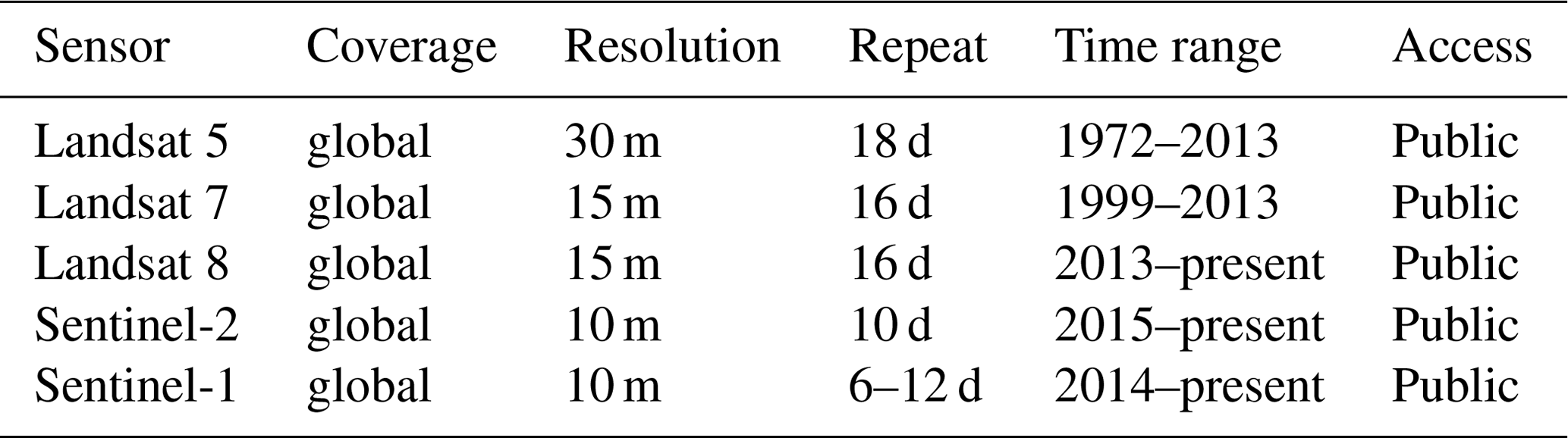
Our data cover five satellites available on Google Earth Engine (GEE; described in detail below); Landsat 5, 7, and 8 and Sentinel-1 and Sentinel-2, with a diverse range of image resolutions, repeat cycles, and operation times (Table 1). Note that GEE only contains Landsat 7 images over Greenland until 2013, although the satellite is still operating as of 2022. As the only satellite operating in winter, Sentinel-1 is essential for analyzing seasonal terminus variations. However, despite the success of Sentinel-1 instruments and their ground processing system in providing open-source data with high geometric accuracy, Sentinel-1 images have several issues. First, apparent georeferencing errors remain between Sentinel-1 and optical images (Ye et al., 2021), thus requiring a georeferencing adjustment for Sentinel-1 that must be automatically applied. Second, the distribution of Sentinel-1 images is not even across Greenland with some glaciers located in between image gaps. Third, as SAR (synthetic aperture radar) images, Sentinel-1 images are cloud-free but suffer from speckle noise (Bamler, 2000), affecting the image quality.
2.2 TermPicks: manually digitized terminus dataset
Deep learning methods employ training data to be used to train the algorithm to predict termini in new imagery. Here, we use a manually picked terminus dataset for Greenland called TermPicks (Goliber et al., 2022), which covers 291 outlet glaciers in Greenland with over 39 000 terminus traces spanning the period from 1916 to 2019. As the most complete set of manually digitized terminus data for Greenland's outlet glaciers, TermPicks enriches the training set and improves the generalization of the model. TermPicks merges several existing glacier ID files across both published literature and several unpublished sources to properly identify glaciers and homogenize terminus trace data. TermPicks data have been cleaned to ensure quality and reformatted specifically for deep learning applications. This dataset covers a wide range of local conditions (e.g., weather, illumination angle, ice mélange strength), glacier orientations, geometries, and satellite sensor differences (e.g., different image textures and pixel value ranges).
2.3 Glacier identifications
Glacier identification is important for data management since Greenland has numerous glaciers. Here, we include 295 outlet glaciers by combining IDs from Moon and Joughin (2008) and TermPicks (Goliber et al., 2022). The criteria of these two IDs are as follows: glaciers with velocities larger than 50 m yr−1, grounding lines below sea level (ocean-terminating), and termini greater than or equal to 1 km in width (Moon and Joughin, 2008; Goliber et al., 2022). To be easily referenced with other datasets, we also include glacier naming schemes cataloged by Bjørk et al. (2015) along with the IDs. Glacier IDs need to be updated continuously because as glaciers retreat, the terminus may diverge into several tributaries and, vice versa, as a glacier advances several tributaries merge into one. Since the two ID files are based on the more recent configuration of GrIS outlet glaciers, some glacier termini do not appear in older Landsat 5 and 7 images because at that time they had merged with adjacent tributaries. Thus, we do not include these glaciers in those older images. Although a static glacier ID is sufficient for current usage, updating the glacier IDs is an essential step in maintaining the longevity of the pipeline in the future (see Sect. 5.5).
2.4 Ice and ocean mask
Land, ice, and ocean masks serve as important data sources for estimating ice-mass balance through elevation changes. Measuring height differences without considering changes in the position of glacier termini can result in significant spurious changes that can dominate estimates of ice-mass change (Kjeldsen et al., 2020; Hansen et al., 2022). Ice masks delineate the glacier area so that measured elevation or mass change can be integrated over the glacier domain (and not, for example, over ocean or rock). In addition, these masks are used to remove measurements over open water so that measured elevation or mass changes never represent, for example, the difference between the height or mass of a glacier and the height or mass of the open water that replaces it when the glacier calves away during retreat.
With the newly generated terminus traces and an original mask, we can update the mask and avoid the spurious changes caused by using fixed terminus positions. The original mask we use is the 2015 GrIMP ice mask from the Greenland Ice Mapping Project (Howat, 2017). This mask used manual delineation of the ice margin from the panchromatic and pan-sharpened multispectral GrIMP 2015 image mosaic (Howat, 2017). The ice mask includes snowfields and identifies the ice sheet margin using visible information and breaks in surface slope where it is visually difficult to differentiate the ice margin. The ocean mask is produced similarly but examines only the coastline with the null of the ice and ocean masks being ice-free terrain (Howat et al., 2014).
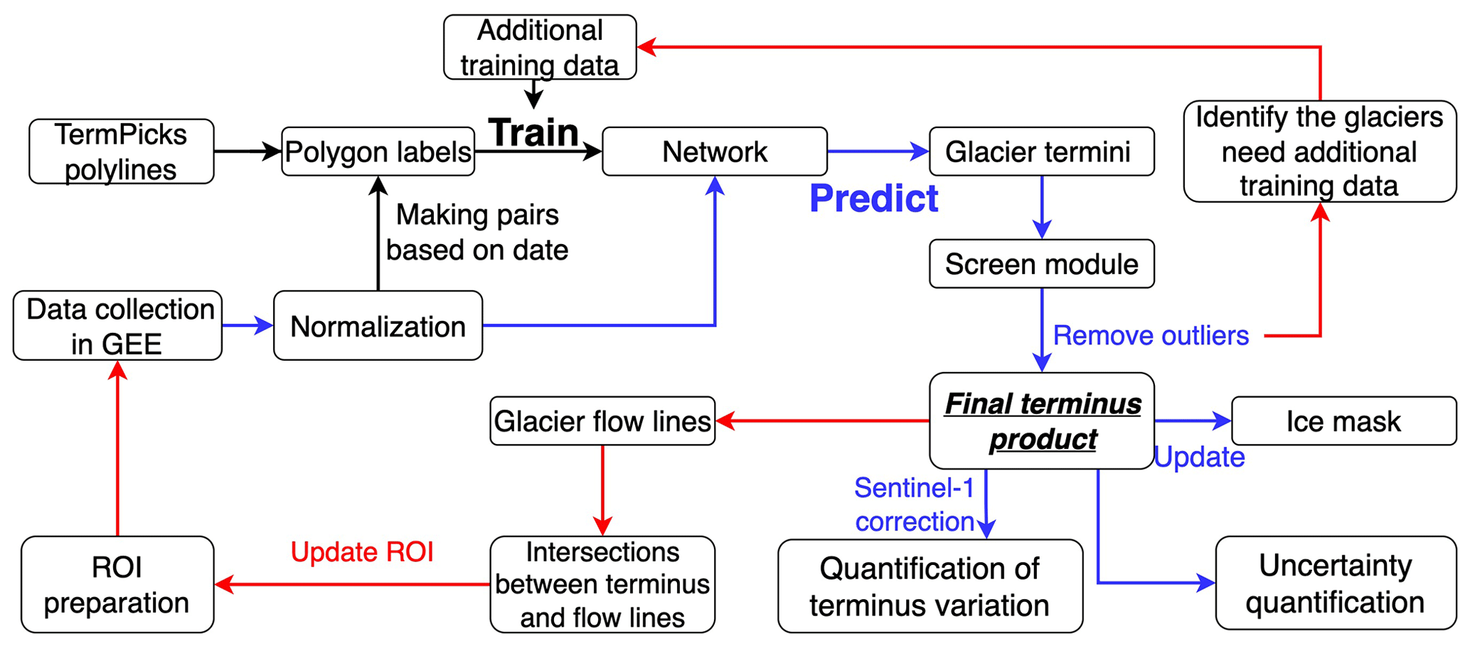
Figure 1Our automated deep learning pipeline. The black arrows represent aspects related to the training data via TermPicks traces and done semi-automatically. The blue arrows represent the procedures that are fully automated when generating glacier terminus traces. The red arrows represent the procedures in the workflow emplaced to maintain the longevity of producing terminus traces through automation.
Our overarching approach is to build an automated pipeline (Fig. 1) for extracting outlet glacier termini from all available satellite remote-sensing images on Google Earth Engine over Greenland using deep learning (DL). Automation requires steps above and beyond terminus delineation, including image collection, pre-processing, quality control, and uncertainty quantification (Fig. 1, blue arrows). Additionally, converting the TermPicks terminus data into a training dataset suitable for deep learning highly generalizes the model and ensures the success of extracting glacier termini from new datasets (Fig. 1, black arrows). In the long term, additional efforts are required to maintain the pipeline, such as preparing more training data and updating the region of interest (ROI) (Fig. 1, red arrows). We adopt similar post-processing procedures with Zhang et al. (2019) that vectorize deep learning output to generate terminus traces. The whole pipeline is built and executed with all software written in Python and Bash.
The structure of the method section follows the order of data processing. We first collect remote-sensing images and conduct pre-processing (Sect. 3.1). Second, we generate the training dataset by converting the terminus traces in TermPicks into label polygons and pairing polygons with the remote-sensing images (Sect. 3.2). Third, we introduce the model architecture and the training progress in Sect. 3.3. Fourth, Sect. 3.4 to 3.6 are post-processing procedures after applying the well-trained model to make inferences on all the images collected via Google Earth Engine. Finally, we update the ice and ocean mask with the newly generated glacier termini (Sect. 3.7).
Table 1Satellite missions with publicly available data on Google Earth Engine for terminus extraction.
3.1 Automated data collection and pre-processing
As the first step, automating image collection eliminates the time involved in the manual collection of remote-sensing imagery. We use the Google Earth Engine (GEE) Python application programming interface (API) (https://earthengine.google.com/, last access: 21 August 2023) to automate our search for satellite data with a given ROI for each glacier and use GEE tools (https://github.com/gee-community/gee_tools, last access: 21 August 2023) to automate data collection. The ROIs are bounding boxes, which require manual preparation to span the range of terminus variations occurring during the study period for each glacier. This is the only manual step in data collection; however, it only needs to be done once for each glacier and thus represents the minimum manual effort. GEE provides a platform for scientific analysis and visualization of geospatial datasets but also hosts a large volume of satellite imagery that goes back more than 40 years and stores these in a public data archive (Table 1). The images, ingested on a daily basis, are then made available for global-scale data mining. GEE also provides APIs and other tools to enable the analysis of large datasets. Through the fusion of multiple datasets on GEE, we can provide a publicly available, densely sampled terminus position dataset that covers the observational time period and importantly fills gaps in existing (manual and automatically delineated) terminus datasets. We do not use a cloud filter to maximize the number of available images where termini may be visible. This is because common cloud filters are calculated based on the full image scene but not the area of interest where a terminus might be located. Thus, image scenes with high cloud coverage might still have clear views of glacier termini. Instead, we filter cloud-covered termini with a screening module described in Sect. 3.4. Overall, we collected ∼430 000 images with a total volume of ∼1 TB spanning the GrIS over a period from 1984–2021.
In addition to automating the data acquisition process, we also automate several data preparation steps before applying DL to delineate glacier termini. First, all satellite images are cropped to the ROI on the GEE platform to save local processing and storage costs. For example, the size of an entire Sentinel-1 scene is about 800 MB, while the size of a cropped image is less than 10 MB, meaning that cropping can decrease costs by a factor of ∼80. Second, we pre-process these cropped images on our local server to normalize image differences between sensors with heterogeneous image textures, resolutions, pixel values, etc. This normalization is necessary since it will ease the terminus extraction task for the DL algorithm by decreasing the complexity level of the dataset, especially when applying DL to a substantial volume of images. We first use histogram normalization to equalize the pixel value differences between SAR and optical image types with different dynamic ranges and image textures (Zhang et al., 2021). We then normalize the image size, which is commonly adopted in the computer vision field for better capturing object features with various physical sizes (Xu et al., 2017). The size normalization allows glaciers with various natural sizes to have a similar image size in computer vision, which largely decreases the complexity of delineating the glacier terminus. In other words, the normalization makes small glaciers appear to the deep learning model as if they had a similar physical size. Specifically, we upsample small images (image width less than 1000 pixels) by an integer value using cubic interpolation so that their widths are just over 1000 pixels. We do not downsample images of large glaciers to avoid losing spatial information. Moreover, since the images will be subdivided into patches with overlaps before going through the model (Zhang et al., 2019), upsampling the small images allows the model to make multiple predictions over the same area, making the inferences more robust. The effect of size normalization will be discussed in Sect. 5.1.
Figure 2An example of converting a polyline into a polygon label and producing a labeled figure. (a) The source image, TermPicks traces (red curves), and the reference polygon for this glacier (blue polygon). The terminus of the reference polygon is upglacier from all the TermPicks traces. (b) The red polygon shows a converted polygon label from one of the TermPicks traces, and the binary label image is derived from the polygon.
3.2 Generating training data from TermPicks
The ability of the model to generalize and identify a glacier terminus is primarily determined by the heterogeneity found in the training dataset (LeCun et al., 2015). More precisely, we want the training dataset to reflect the heterogeneity of conditions observed in the real world. To accomplish this, we leverage existing manually picked terminus data from Greenland using TermPicks (Goliber et al., 2022), which consists of the largest compilation of manually picked terminus traces covering a range of satellite sensors and glacier conditions. The TermPicks traces, which are polylines, need to be converted into labeled polygons for generating binary labels (Fig. 2) for each glacier in Greenland. Each labeled polygon contains the glacier terminus, fjord boundary, and an outer boundary that ensures that the polygon covers the corresponding source image. To automate the conversion of terminus traces into polygon labels, we manually create one reference polygon for each glacier. A reference polygon is similar to a polygon label, but its terminus (blue polygon in Fig. 2a) is up-glacier from all the TermPicks traces (red curves in Fig. 2a) for that glacier. This ensures that each reference polygon has two intersections with a TermPicks trace (on either end of the TermPicks trace). We then generate polygon labels by connecting each TermPicks trace between the two intersection points and the reference polygon (e.g., red polygon in Fig. 2b). Then, we pair the converted polygon labels with the GEE collection of satellite images based on date. Finally, we manually abandon training data mismatches between polygon labels and images. This can occur when manually picked traces do not extend across the fjord, contain erroneous points (Fig. S1a, b in the Supplement), and/or are offset due to differences in georeferencing (Fig. S1c). After manual checking, we have 16 440 polygon labels from TermPicks for 249 glaciers. Most of the unused TermPicks traces are due to not being able to match the source image, as we only use the data available on GEE, which has a limited temporal range.
Although TermPicks covers a range of conditions and brings great diversity to the training set, additional training data would presumably improve the accuracy of the model in difficult situations. We identify five conditions that pose distinct challenges: (1) images covered by cloud but where termini are still visible; (2) winter Sentinel-1 images with blurry boundaries due to their coarse resolution, ice mélange, and snow cover; (3) images with shadow over the terminus; (4) images with tabular icebergs close to the glacier terminus; and (5) similarities in texture between ice mélange and glacier (Fig. S2). For these types of images, we manually prepare an additional 1466 training examples. To further increase the diversity of our training set, we perform data augmentation for all the training examples, including rotating images by 90, 180, and 270∘, and image flipping following (Zhang et al., 2019), increasing the training set by a factor of 4.
3.3 The architecture and training of deep learning model
We use DeepLabv3+, a state-of-the-art deep learning algorithm for image segmentation (Chen et al., 2018). DeepLabv3+ combines an encoder–decoder architecture with atrous spatial pyramid pooling, where the former can obtain sharp object boundaries while the latter senses multi-scale contextual information. Sharp boundaries can improve delineation accuracy, and sensing multi-scale information helps indirectly when we integrate remote-sensing datasets with different spatial resolutions. This model architecture has been proven to have a large learning capability (Chen et al., 2018), spatial transferability, and the capability of using multi-sensor remote-sensing images (Zhang et al., 2021). To train the model, we use binary cross entropy as the loss function and a stochastic gradient descent method as the optimizer with an L2 regularization factor of , as recommended by Zhang et al. (2021). Based on the learning rate in Chen et al. (2018) and Zhang et al. (2021), we train the model with learning rates of , , and and choose owing to its lowest validation loss. To improve the efficiency of model training, we choose the largest possible batch size (16) on four A100 GPUs with 160 GB GPU memory in total. We set the batch size to a power of 2 to take full advantage of GPU processing (Kandel and Castelli, 2020). From TermPicks traces, we randomly select 100 traces as the test set and take the rest into the training set. Among the training data, we randomly select 5 % as the validation data to conduct early stopping in order to mitigate overfitting. The training will be stopped when the validation error stops decreasing for three consecutive epochs. The model training took seven epochs, about 1 week, and consumed 120 GB of memory. After the training, we apply the well-trained model to the test set in order to quantify the test error and to all the images collected via GEE in order to generate the terminus dataset. We measure the test error by calculating the enclosed area bounded by the TermPicks traces and the model predictions divided by the length of the TermPicks traces. In the case where there are crosses between a TermPicks trace and a model prediction, we calculate the area on both sides of the crosses and then add them together. Terminus picking and post-processing for a single image takes less than 1 min.
3.4 Automated screen module
Despite the power of deep learning technology, it cannot perfectly identify termini for all available images. Moreover, the model is expected to generate erroneous results from images where termini are invisible. These results should be detected and removed. With this in mind, we have developed an automated screening module to assist with quality control. Many previous DL methods applied to terminus delineation do not have quality control (Mohajerani et al., 2019; Zhang et al., 2019). Where it does exist, data screening has been simplistic and not automatically applied. For example, Zhang et al. (2021) only considers the complexity of the terminus shape and removes traces with abnormal complexity (which, in turn, requires a threshold to be established for each glacier), Baumhoer et al. (2019) only considers outliers that arise in a time series of terminus position change over time, and Gourmelon et al. (2022) remove the outliers based on terminus length. Cheng et al. (2020), however, did design an automated data screening based on the deviation of two classifications from the model. Our screening module is based on using the physical properties of glacier termini.
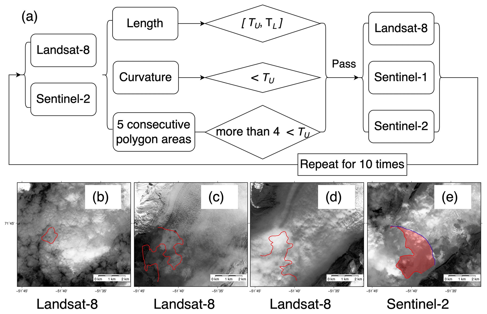
Figure 3(a) The pipeline of the screening module. TU is the upper threshold, and TL is the lower threshold. Each metric (length, curvature, five consecutive areas) has its own threshold. Only the results from optical images are used to calculate the thresholds, and the thresholds are applied uniformly to all the datasets. Examples of results abandoned for different reasons. (b) Short terminus. (c, d) Long and complex terminus. (e) Terminus forms a large polygon with its adjacent picks. The backgrounds are the source images of the wrong picks. The red line in (e) is the wrong pick, and the blue curve shows its time-adjacent manual pick.
Based on the previous work (Zhang et al., 2021; Baumhoer et al., 2019; Gourmelon et al., 2022), we develop an automated screening module that forgoes any manual intervention or prior knowledge of the data (Fig. 3). The outliers are quantified in three different categories: (1) the number of intersections between terminus and glacier flow line, (2) terminus length, (3) terminus curvature, and (4) the abnormally large area enclosed by the two temporally closest termini. This latter case refers to outliers in a time series of terminus change. Terminus curvature is computed among every three adjacent points along the terminus based on Peijin Zhang's work (Zhang, 2018), and then an average is taken for each terminus trace. Finally, we calculate the area enclosed by two temporally adjacent termini to determine the change in glacier area over time. We will only keep termini that have a single intersection with the glacier flow line. For each of the last three metrics, we calculate the lower (TL) and upper thresholds (TU) based on the interquartile range:
where Q3 is the 75th percentile and Q1 is the 25th percentile of the data range. The thresholds are calculated automatically based on the results of the same glacier and the same satellite. Since the Sentinel-1 images suffer from speckle noise, Landsat 7 is affected by SLC-off (scan-line corrector off), and Landsat 5 has a small number of images, the results generated from these satellites are of relatively poor quality compared to the other datasets, or the obtained thresholds are inappropriate. Therefore, we calculate the thresholds based on results from Landsat 8 and Sentinel-2 and apply them uniformly to all remaining datasets. For outliers in terminus length, we remove both the lower and upper thresholds (Eqs. 1 and 2) because we do not anticipate large changes in terminus length in either direction (bigger or smaller). In contrast, terminus curvature and area change outliers are only removed with the upper threshold (Eq. 1). This is because high-quality terminus traces are expected to be smooth with little curvature and have a time derivative of terminus change that is small at the sampling frequency permitted. Exceptions to this latter assumption exist when large calving events occur. In that case, if all of the traces are accurate, only one anomalously large area change will occur over a short period (typically less than 1 month). To remove incorrect traces and retain traces providing information on large calving events, we examine the change in the terminus area over five consecutive area polygons (in a moving time window) and remove the first large-area polygon only if more than one large-area change is identified. The removal of outliers changes the data distribution, and we will have new thresholds in the next screening. We repeat this screening procedure 10 times or until we do not find any more outliers to maintain the quality of the terminus product (Fig. 3). Finally, we estimate the success rate by calculating the percentage of the terminus traces that pass the screening module.
3.5 Georeferencing adjustment for Sentinel-1
Location errors occur for Sentinel-1 images along the azimuth direction (Small and Schubert, 2019) introducing error in georeferencing for this sensor in our data (Fig. S3). Although applications have been made to correct these georeferencing errors in post-processing (Ye et al., 2021), they have not been widely deployed for public use. Owing to the overlap of multiple sensors, it is possible to have more than one machine-predicted terminus trace for a single date, allowing us to use duplicate traces to aid in performing a georeferencing adjustment for Sentinel-1. This is done by calculating all of the areas enclosed by Sentinel-1 traces and comparing these to area enclosed by traces on the same day, but from optical sensors. Then we take the averaged area difference between these two time series to adjust the georeferencing offset in the retreat time series.
3.6 Uncertainty quantification
Traditional uncertainty quantification for glacier terminus position is conducted by calculating the difference between manually picked termini and automatically picked termini (e.g., Cheng et al., 2020). However, the model accuracy likely varies over time as glaciers experience different conditions (e.g., cloud cover). Uncertainty quantification thus requires significant manual effort to ensure that the computed uncertainty is representative of such variability. We compute the uncertainty in two ways. First, we use duplicate traces (described above) to automatically quantify the uncertainties for each glacier. For this, only the traces with the highest source image resolution (Table 1) are kept (Sentinel-2 and Landsat 8). We do not use duplicate Sentinel-1 traces because they are used for the georeferencing offset for that sensor, and we do not use Landsat 5 or 7 because of the lack of overlap with other datasets. Uncertainty from duplicate traces is computed by comparing the average area enclosed by the duplicate Landsat 8 traces and Sentinel-2 traces for the same date. For each glacier, we average the uncertainties from all duplicated traces and use the mean to represent the uncertainty in that glacier. We also divide this area by the piecewise terminus length to get the uncertainty in terminus position as a measure of length change. This is done because some data users may prefer to examine terminus change in length instead of terminus change in area.
We also compute uncertainty through deploying the Monte Carlo (MC) dropout (Gal and Ghahramani, 2016) method, which has become widely adopted in the uncertainty quantification for DL methods (Abdar et al., 2021). Dropout is a regularization technique that prevents overfitting of the data ensuring that the model works well with new imagery that is not contained in the training data. MC dropout yields variants of our DL model by dropping out random subsets of the model's neurons during prediction (setting their values to zero). These variants make multiple inferences for a single remote-sensing image, and the differences between these inferences can be used to quantify the model uncertainty. Hartmann et al. (2021) applied MC dropout to glacier terminus delineation and built a two-stage approach. They used the uncertainty in the first model as additional information to train the second model. The multiple outputs of the second model are averaged to eliminate the uncertainty and get the final prediction. Here, we deploy MC dropout and use model variants to pick multiple terminus traces for a single image. By quantifying the average difference between the traces from the original model and the variants, we measure the uncertainties in the terminus position, providing a different perspective on uncertainty quantification from duplicate traces. MC dropout requires multiple inferences and is computationally time-consuming. To strike a balance between computational cost and the reliability of the MC dropout, we randomly chose 10 images from each of the five sensors and made three inferences for each of the images. Thus, in total, each glacier will have six measures of uncertainty: one from duplicate traces and the other five estimated by MC dropout for each sensor.
3.7 Ice and ocean masks
The newly generated terminus traces are also used to update the GrIMP mask for accurate estimates of ice-mass balance. While we can update masks monthly, we do not expect significant changes in glacier area on this timescale. We thus only create updated masks annually beginning in 2018 to serve the ICESat-2 community needs for improved accuracy of laser returns during periods of extensive glacier terminus retreat. To create a new ice mask we first select terminus traces at a time of minimum ice extent (late fall) for every glacier. These termini are combined with geometries delineating the edges of outlet fjords and the edges of static ice margins from GrIMP (Howat et al., 2014) to form a continuous boundary of the ice sheet. We use the new terminus to update only the ocean mask and consider the bedrock mask to be static. The ice mask is updated automatically because of the shared ice–ocean boundary with the ocean mask. Practically, we first vectorize the ocean mask into a shapefile. Second, we crop the shapefile with the glacier ROIs and replace the parts in the ROIs with the newly generated terminus traces. Then, we convert the updated shapefile to a raster as the new ocean mask. Finally, the residual of the new ocean mask and original bed mask serve as the new ice mask.
In addition to terminus delineation, we have successfully automated data collection, pre-processing, data quality control (Fig. 3), uncertainty quantification, the measurement of terminus variation (Fig. 1, blue color), and the derivation of annual land, ice, and ocean masks for Greenland. The improvements in automation enable the pipeline to generate a tremendous number of terminus trace data continuously with controlled quality and measured uncertainties. As a result, the pipeline can automatically produce new terminus traces from all newly acquired satellite images in Greenland.
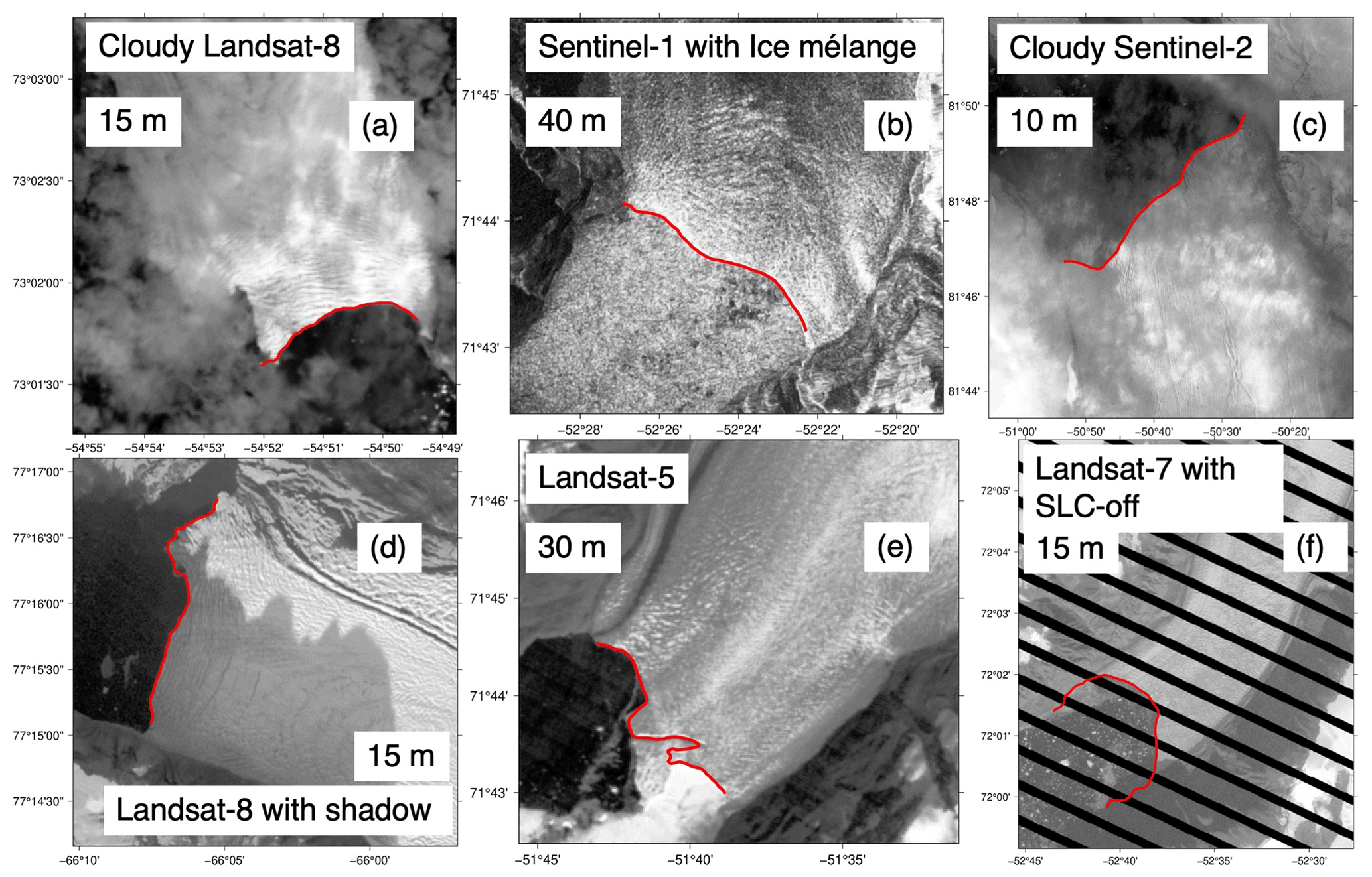
Figure 4Examples of the automatically picked glacier terminus. The model can handle different scales and resolutions, light cloud cover (a, c), ice mélange (b), heavy shadowing (d), complex geometry (e), and Landsat 7 scan-line errors (f). All the results are beyond the training set.
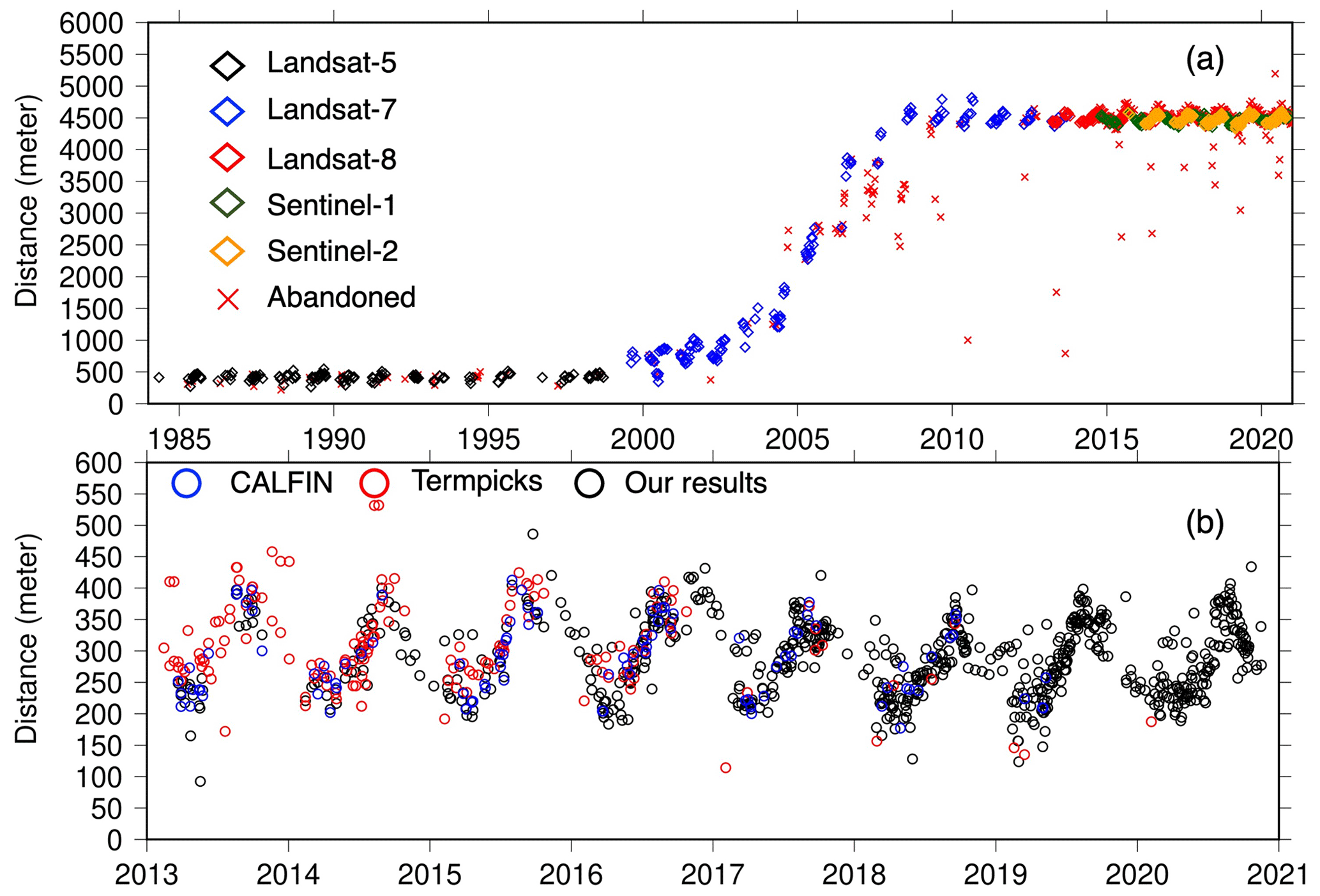
Figure 5(a) An example of terminus variation over time from our results showing clear seasonal and longer-term signals in terminus change. We highlight the ability of our screening module to detect erroneous traces (red x signs). After 2014, seasonal variations are more apparent owing to the addition of wintertime records from Sentinel-1. (b) Detail of (a) over 2013–2021 showing the comparison between our results and manual traces from TermPicks covering 2013–2020 (Goliber et al., 2022) and CALFIN covering 2013–2019 (Cheng et al., 2020).
4.1 Data quality
Our model is capable of handling different image scales and resolutions, heavy shadowing, ice mélange, light cloud cover, and Landsat 7 scan-line errors (Fig. 4). Thus we can pick the terminus trace whenever it can be clearly seen in an image. Further, our screening module is capable of removing erroneous terminus traces with numerous causes (e.g., cloud cover, image resolution, Fig. 3). With these removed, a time series of terminus variation shows clear signals without spurious changes in terminus position (Fig. 5). Data quality is assessed via test error, success rate, and uncertainty. The test error provides a general estimation of the model's performance. Our averaged test error is 79 m (Table S1 in the Supplement), which is comparable to previous studies where errors range from 33 to 108 m (Mohajerani et al., 2019; Zhang et al., 2019; Baumhoer et al., 2019; Cheng et al., 2020), although the test set and the way of calculating test error are slightly different. Our success rate is determined by examining how many terminus traces pass the screening module and dividing this by the number of images available for each glacier. The success rate of the test set is 90 %, and the test error was reduced to 62 m after the screening module. For the entire dataset, we find an average success rate of 64 % (Fig. 6), but this varies temporally and spatially. Such variations could be caused by the uneven distribution of the training data glaciers with more training data having higher success rates. We have improved the seasonality of the terminus position. However, the model does struggle to delineate termini in many wintertime Sentinel-1 images, probably because of blurry boundaries and the lack of sufficient training data specifically using Sentinel-1 imagery. For example, we only have 484 Sentinel-1 traces from TermPicks and an additional 936 manually prepared Sentinel-1 traces as part of this work. As a result, many more traces from Sentinel-1 images did not pass the screening module (Fig. 7).
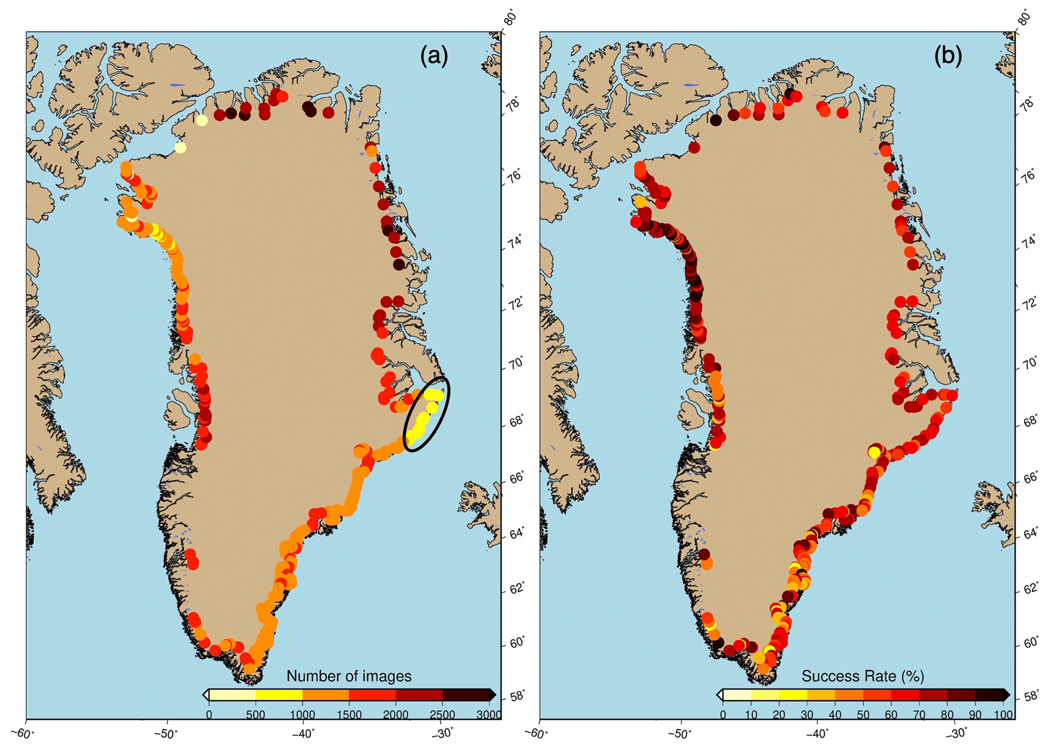
Figure 6(a) Total number of images and (b) overall success rate of AutoTerm for each glacier. The ellipse in (a) indicates the glaciers 127 to 138 with relatively low numbers of images. The spatial variations in image numbers are caused by the variations in satellite spatial coverage. The spatial variations in success rates are caused by the uneven distribution of training data. Glaciers with more training data have higher success rates. The boundary of the GrIS is provided by the Generic Mapping Tools (GMT, https://www.generic-mapping-tools.org/, last access: 21 August 2023).
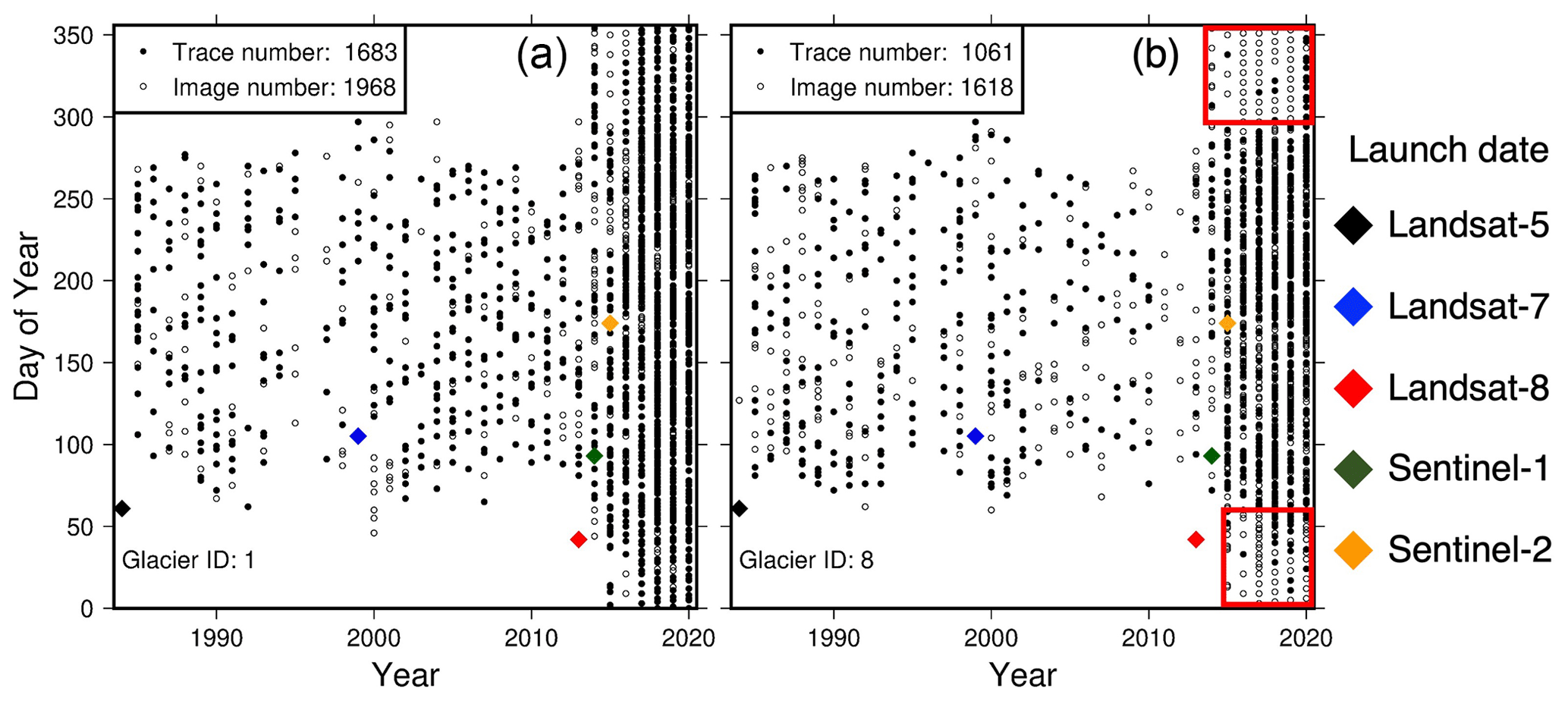
Figure 7Examples of remote-sensing image availability (black dots) versus termini successfully predicted for (a) glacier 1 and (b) glacier 8. The diamonds show the launch date of the satellites. Since 2014, the launch of Sentinel-1 (green diamond) has filled the gap in winters. Due to the blurry boundaries of wintertime Sentinel-1 images, some of these terminus predictions did not pass the screening module (red boxes in b).
The uncertainties are measured in two ways: using duplicate traces and the MC dropout method. The MC dropout measures model uncertainties in neural network parameters, while duplicate traces quantify the performance difference of the model on various datasets. Using duplicate traces, we find an average uncertainty of ∼37 m with a range from 10 to 204 m (Fig. 8a). The duplicate trace uncertainty variation between glaciers along with success rates might be because the training data are not evenly distributed for each glacier; glaciers with less training data will probably have larger uncertainties and lower success rates. Uncertainty also varies across sensor type. Figure 8b–f show the uncertainties in different satellite sensors from MC dropout. Among the five datasets used, Landsat 8 and Sentinel-2 have the lowest average uncertainties, probably because they have the highest spatial resolution. Landsat 7 images suffer from the scan-line corrector (SLC) failure, which contributes to the uncertainties in the derived results. The reasons for the Landsat 5 uncertainty might be twofold. First, Landsat 5 does not have a panchromatic band, and, thus, its resolution is coarser than other Landsat sensors. Second, floating ice tongues were more prevalent at the time of Landsat 5 data acquisition than they are now (Hill et al., 2018), which challenges the model to accurately delineate ice tongue edges without significant training data. The higher uncertainty in Sentinel-1 images could be due to their low image quality, coarse resolution, and the lower volume of training data derived from this sensor. Figure S4 shows multiple predictions of terminus traces resulting from MC dropout with a comparison to the original terminus prediction for two glaciers. Due to the randomness of the model parameter that is shut down during this calculation, MC dropout makes some predictions noisier (Fig. S4a). Further, we observe that prediction noise is larger when the original terminus predictions significantly deviate from reality (Fig. S4b).

Figure 8Terminus trace uncertainties measured by duplicate Landsat 8 and Sentinel-2 traces (a) and MC dropout (f) for each glacier. The averaged uncertainties for all glaciers are shown at the bottom left of each panel. Gray indicates that no uncertainty is measured due to data shortage (either no duplicate trace for panel a or no source image for panels b–f). The boundary of the GrIS is the same as Fig. 6, provided by GMT.
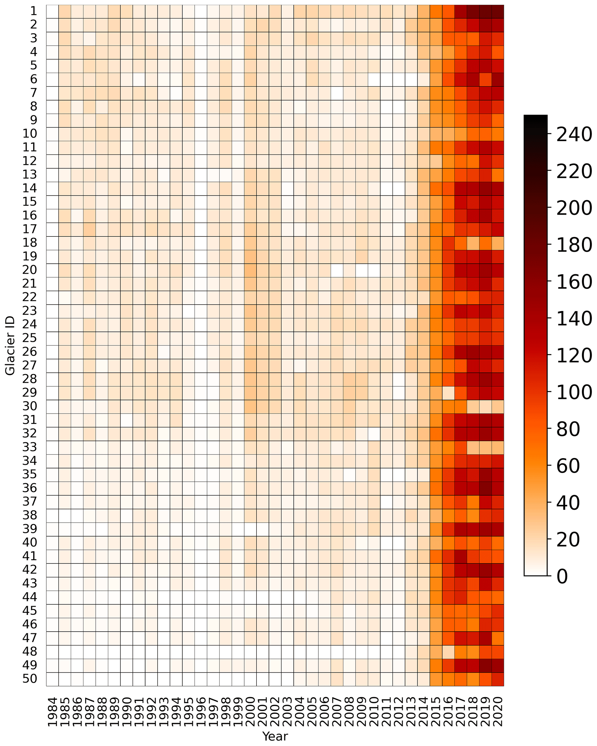
Figure 9Example heatmap of the number of successful traces predicted in each year for glaciers 1–50. The full record of annual trace numbers can be found in the Supplement.
4.2 Data quantity
Using the pipeline, we generated 278 239 glacier termini for 295 glaciers from 433 721 images (Fig. 6). Generally, we find that variations in satellite coverage cause significant spatial variations in image availability. For instance, in central east Greenland (glaciers 127 to 138), the relatively low number of images is caused by the shortage of Sentinel-1 images in this region. There are only ∼60 Sentinel-1 images in total for each of these glaciers, while other glaciers have 300–600 images available. We also find the launch of Landsat 8, Sentinel-1, and Sentinel-2 greatly improve the frequency of remote-sensing images (Fig. 7) providing ∼100 traces per year per glacier for the most recent (>2014) period. Figure 9 shows a heatmap of terminus traces for selected glaciers. The Supplement provides similar heatmaps for the full record of glaciers (Figs. S6–S10). Importantly, Sentinel-1 images fill data gaps in winter when optical sensors struggle with low-light conditions. These wintertime terminus picks provide near-continuous characterization of the seasonality of terminus position (Fig. 10).
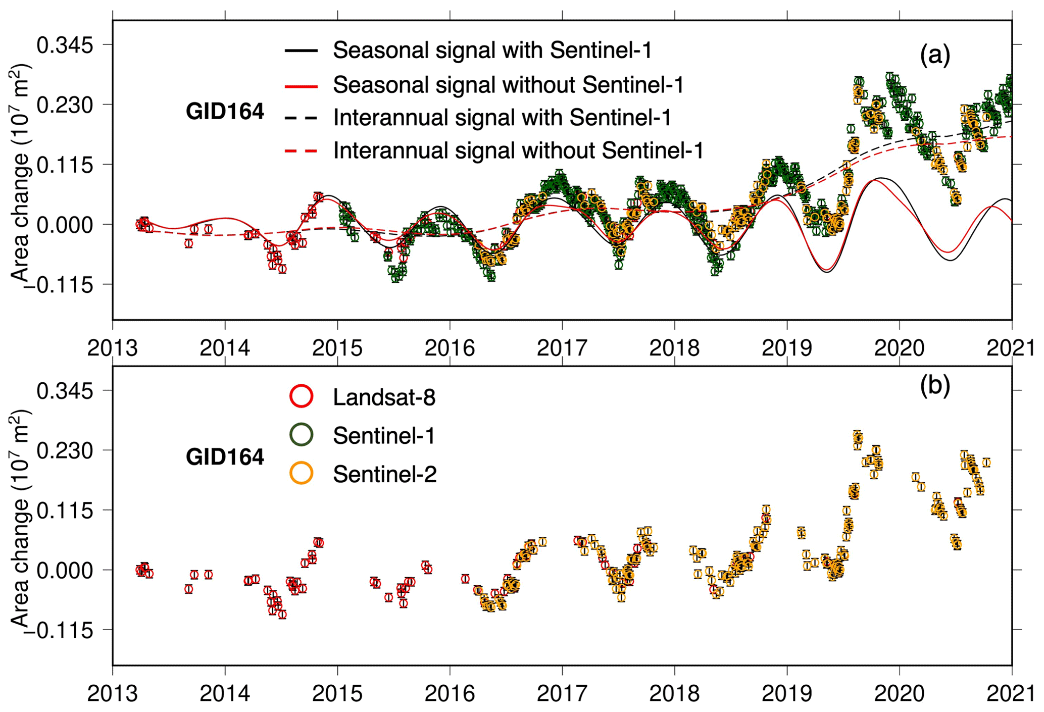
Figure 10An example showing the importance of including Sentinel-1 traces for glacier ID 164. (a) With Sentinel-1 (green circles), Landsat 8 (red circles), and Sentinel-2 (orange) and (b) with only Landsat 8 and Sentinel-2 data. In (a), we quantify the inter-annual and seasonal variation in terminus position using the singular spectrum analysis method (Zhang et al., 2018). Uncertainties are shown as vertical bars for each terminus trace and are measured by duplicate traces. Legends in (b) are shared by both panels (a) and (b).
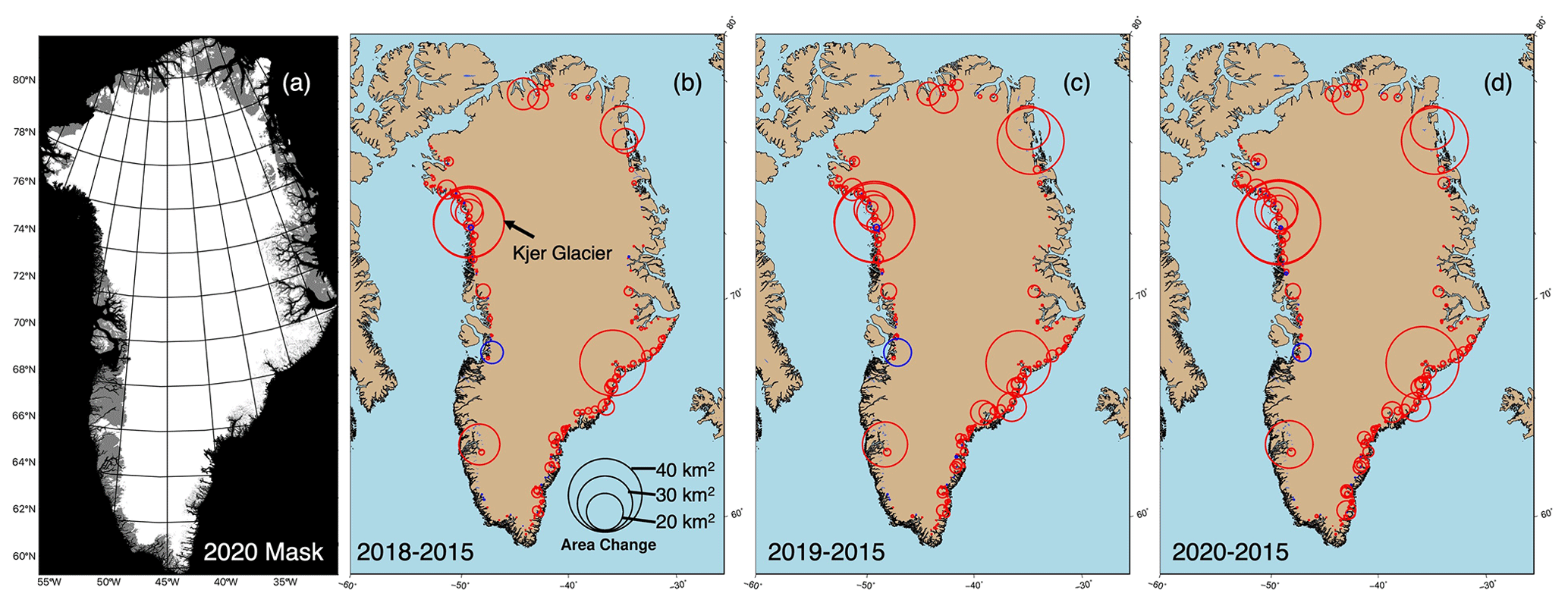
Figure 11An example of an updated ice mask for 2020 (a) and the terminus change between the updated masks and the original 2015 GrIMP ice mask (b–d; 2018–2020). Red circles represent retreating glaciers and blue circles represent advancing glaciers. The size of the circle indicates the difference in area change in each glacier from the original mask. The boundary of the GrIS in (b–d) is the same as Fig. 6, provided by GMT.
4.3 Ice mask
In addition to terminus trace data, we also generate three new ice, ocean, and bedrock masks for 2018, 2019, and 2020 (Fig. 11). Each newly generated ice mask is provided as a single GeoTIFF file with black representing the ocean, gray representing the bedrock, and white representing the ice (Fig. 11a). To identify how valuable updates to the ice masks are, we compare our masks with the 2015 GrIMP ice mask product (Howat et al., 2014) for each year (Fig. 11b–d). We find ongoing retreat of most glaciers after 2018 with glaciers in the northwest and southeast of Greenland dominating the retreating. The net area change in ice extent is 520 km2 for 2018, 660 km2 for 2019, and 72 km2 for 2020. The largest area change was 45.5 km2 at Kjer Glacier, which was previously attached to a nunatak and has now detached from it and diverged into two tributaries (glacier IDs 28 and 29). The one blue circle in Fig. 11b shows the advance of Jakobshavn Isbræ (Sermeq Kujalleq), which has been associated with regional cooling of ocean water (Khazendar et al., 2019; Joughin et al., 2019).
4.4 Data format
AutoTerm contains shapefiles of terminus traces and four supplementary data, including (1) a complete record of uncertainties, (2) identification of glaciers, (3) temporal coverage of terminus traces, (4) time series of terminus variations, and (5) ice masks. The terminus traces of a particular glacier are assembled in a single shapefile with an attribute table showing the metadata of each trace. The metadata contain the date in YYYY-MM-DD format, glacier ID, source image satellite, and the uncertainty of each trace by averaging the two types of uncertainties provided. The entire record of uncertainties is provided in a spreadsheet. Each glacier has six averaged uncertainty measures, including one from duplicate trace uncertainty and five from MC dropout uncertainties in different satellites. Data end users can choose an average of the two uncertainty measures as a total uncertainty or use one uncertainty value from the spreadsheet based on the prevalence of the data type used. The identification file includes the glacier location, ID, name, and region of interest. For each glacier, we will provide a figure similar to Fig. 7 showing the temporal coverage of terminus traces and a time series figure identical to Fig. 5 showing the terminus variation. The temporal coverage and time series figures will be packaged into two KMZ files, respectively. In the KMZ files, the figures are assigned with the locations of their corresponding glaciers. By doing so, we can easily access the information on data gaps and terminus variation, comparing adjacent glaciers. The format of ice masks is described in Sect. 4.3.
5.1 Methodological improvements
Building on previous DL-based studies, the major improvements we achieve in this work are (1) increasing the generalization level of the deep learning model to enable more and better quality terminus predictions, (2) deploying size normalization to improve the accuracy of terminus delineation for small glaciers, (3) designing a rigorous automated screening module to control the data quality, and (4) automating several additional steps in the pipeline such as data collection and uncertainty quantification to allow the data to be regularly delivered.
The substantial generalization improvement we observe is due in large part to converting the TermPicks (Goliber et al., 2022) dataset into a rich training dataset. All previous DL-based studies use training data that are manually prepared by the individual authors with CALFIN having the most training data (1773 training pairs; Cheng et al., 2020). Because model generalization is tied to the diversity of training data, small volumes of training data limit the ability of the model to generalize and thus reduce the accuracy of terminus predictions. Instead, we prepare the training data semi-automatically and only manually check for mismatches between TermPicks traces and the source images, saving time. Further, TermPicks covers a larger variety of glacier conditions, geometries, and satellite sensor differences. In total, we have 16 440 training pairs from TermPicks and 1466 training examples prepared manually. This diversity is much more representative of the real world and improves the success of the model. To demonstrate the generalization brought by TermPicks, we train the model with only 1466 training examples prepared manually. That model has a test error of 315 m and a success rate of 46 %, while the model trained with TermPicks has a testing error of 79 m and a success rate of 90 %.
Despite numerous studies that have demonstrated the feasibility of using DL algorithms to automate terminus delineation, there is an additional degree of automation needed to deal with the emerging big data now available on cloud services. Our automated pipeline saves substantial manual effort, even though we still employ some manual effort, like preparing the regions of interest. As the volume of images increases, so does the difficulty for the model to succeed on all of them. As a result, the need for quality control becomes paramount, particularly given that there are plans for follow-on Landsat missions extending terminus time series indefinitely into the future. Although we could devote more effort to manually preparing additional training examples and improving the model accuracy, we opted to build a screening module enabling improved data quality. This choice results in significant time savings over adding additional training data. Terminus data produced from machine learning will always have larger uncertainty than manually delineated data since we use manually delineated data as our training data. The uncertainty in data generated from deep learning has been traditionally quantified by measuring the difference between automatically picked termini and manually picked ones, which is rigorous but also requires significant manual effort. Further, how representative such uncertainty is depends on the diversity of conditions covered by manual delineations. As a result, improved uncertainty estimates come at the cost of labor required to compute them. Our implementation of duplicate traces and MC dropout provides an estimate of uncertainty automatically while only sacrificing a modest amount of rigor over manual delineation. For instance, if both duplicated traces deviate from reality but are close to each other, the uncertainty would not represent reality.
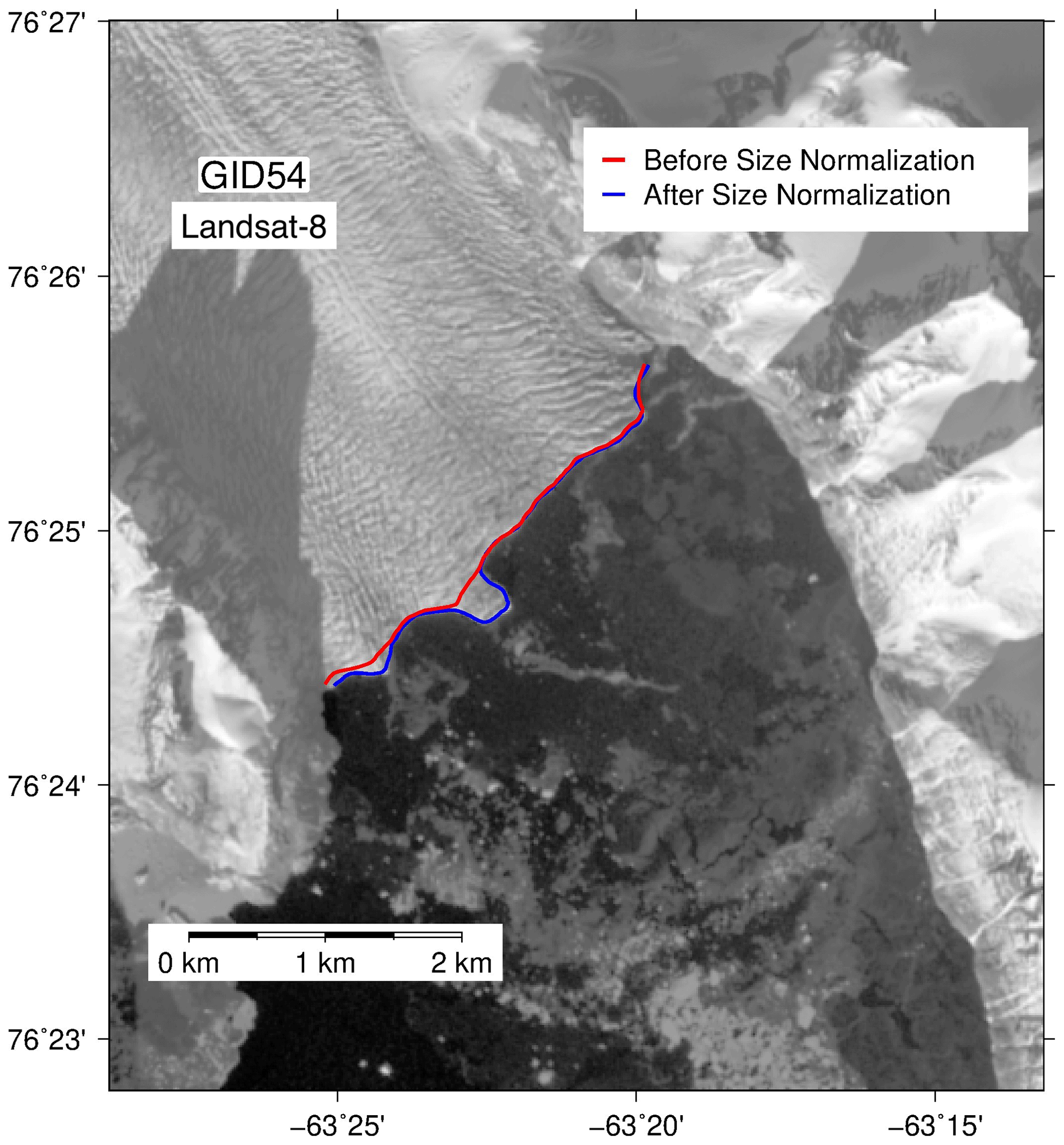
Figure 12An example showing the effect of size normalization for glacier ID 54. After normalization, delineation of the terminus is more accurate and captures small features.
Image normalization homogenizes images and thus eases the difficulties of terminus delineation under various conditions (e.g., weather, illumination, geometry). In addition to histogram normalization (Zhang et al., 2021), we also conduct size normalization to deal with the diversity of glacier sizes around Greenland. Although the design of DeepLabV3+ enables the model to sense multi-scale contextual information, glacier sizes in Greenland vary by orders of magnitude (1–80 km in width), necessitating size normalization. Since we upsample small images, size normalization is especially useful in increasing the accuracy of terminus predictions for small glaciers and capturing detailed features in the terminus (Fig. 12). We randomly select 36 images of five small glaciers as the test set for size normalization. These images are beyond the training set. Table S3 shows that the size normalization effectively decreases the test error for all five glaciers. We estimate the uncertainties from all duplicated traces of that five glaciers, which also reveals the effectiveness of the size normalization (Table S3).
5.2 Advantages of AutoTerm
Owing to the automation level we have achieved, AutoTerm produces terminus data with complete spatial coverage, sub-seasonal sampling interval (Fig. 9), and full-width terminus morphology. Previous studies on terminus variation either have a high temporal resolution (Schild and Hamilton, 2013; Kehrl et al., 2017; Fried et al., 2018; Catania et al., 2018) or complete spatial coverage (Murray et al., 2015; Wood et al., 2021) but not both because of the laborious effort required with manual terminus delineation. Even with DL-based terminus prediction, most data available comes from CALFIN (Cheng et al., 2020), which produced 22 678 terminus traces across 66 Greenland glaciers, limited in part because they only examined Landsat imagery. Our inclusion of Sentinel-1 data improves the temporal sampling of the terminus data 3-fold over CALFIN, providing an average sampling frequency of ∼100 traces per year for the most recent (>2014) period (Figs. 5b and 10). These additional winter terminus traces allow improved accuracy for quantifying seasonality and inter-annual variability (Fig. 10). Further, our ability to provide full-width terminus trace morphology enables a detailed investigation of the specific processes controlling the ice–ocean interface (Murray et al., 2015; Fried et al., 2018; Rignot et al., 2016; Slater et al., 2021).
5.3 Limitations
Despite the success in automating the pipeline and producing a massive number of terminus trace data, our workflow is limited by the immense computational power (120 GB of GPU memory) and long training time (5–7 d) required, which also make uncertainty quantification challenging. This degree of processing time is due to the extensive volume of training data, which are crucial to generalizing the model and improving model performance. The second limitation is caused by our assumption that the screening module provides high-quality results. This assumption rests on the choice of thresholds defined by the interquartile range in the screening module. Thus, when most results for a glacier are not credible, the screening module might not be able to clean the results because the random distribution of the terminus attributes leads to improper thresholds. The resulting terminus variation series could be spurious, and additional training data or a more advanced model will be required to improve the data quality. The third limitation is that even though we include additional training data, the model might struggle with some challenging situations (Fig. S2). The fourth limitation is that further validation will be needed to apply it globally despite the success of the screening module in Greenland. The fifth limitation comes from the biased value of duplicate uncertainty as Landsat 8 and Sentinel-2 images have the highest resolution among the five satellites. A final limitation is that not all the data that can provide terminus trace information are included here. For example, there are numerous satellite and airborne sensors that are not available on GEE (e.g., air photos, ASTER, and other SAR products). Our workflow is limited to what is available on GEE. As a result, AutoTerm only produces a high sampling frequency with winter traces after 2014.
5.4 Difference between the two types of uncertainties
The differences in the two types of uncertainties are caused by their quantification methods and source images. When using MC dropout to quantify uncertainty, the model varies, but the input images are fixed, while the situation is reversed when we quantify uncertainty measured by duplicate traces. As a result, the MC dropout uncertainty emphasizes uncertainty in the model itself, while duplicate traces rely on data uncertainty inferred from the difference between Landsat 8 and Sentinel-2 imagery. Additionally, the MC dropout uncertainty permits quantification of uncertainty for each dataset and is thus influenced by the characteristics of the training data as a whole, such as the SLC failure in Landsat 7. On the contrary, the uncertainty from duplicate traces is more representative of Landsat 7 and Sentinel-2 than other datasets. Since Landsat 8 and Sentinel-2 images have the highest resolution among the five satellites, using the duplicate uncertainty to represent the error of results obtained from other satellites would be biased towards lower values. Moreover, different ways of choosing source images in two types of uncertainties bring discrepancies. The source images for computing the MC dropout are randomly selected, but this is not true for duplicate traces. The dates having duplicate traces from both Landsat 8 and Sentinel-2 images are governed by satellite coverage. Overall, uncertainties from MC dropout and duplicate traces are roughly equivalent, especially for Landsat 8 and Sentinel-2 results since duplicate trace uncertainties are also based on these two satellites (Fig. S5).
5.5 Future effort required for maintaining the pipeline
Maintaining the longevity of the pipeline is essential as glaciers and ice sheets in our chosen regions undergo rapid and large-scale changes with time. To continuously produce terminus traces each year in the future, the ROI for each glacier can be automatically updated based on the intersection between the glacier centerline and the most recent terminus trace. With an updated ROI, new images can be collected via GEE and the entire pipeline can be rerun to produce new terminus trace data for that year. Moreover, manually preparing additional training data might be required as the model could fail to pick the terminus from new images. The model's failure will result in many termini not passing the screening and high uncertainty. The pipeline can use the low success rates and high uncertainty to alert us to prepare more training data for the corresponding glaciers. Annually, these terminus data can be used to calculate updated glacier terminus change data, which in turn inform the need for the generation of new land, ice, and ocean masks. We can also update glacier ID files triggered by the bifurcation or confluence of termini. For example, when a glacier retreats and, in doing so, diverges into several tributaries or when an ice shelf collapses and exposes new glacier termini, the existing glacier IDs (numbers) can be suffixed with letters (a, b, c, etc.) indicating that the origin of each tributary is embedded within the ID. When several tributaries merge into one main terminus, for example through advance, the ID of the largest tributary will be kept. Lastly, we depend on future community feedback about our products to assist in identifying issues not caught by our screening module. This is because the massive number of data precludes the ability to guarantee the quality of each individual trace.
This study builds a fully automated, deep-learning-based pipeline that can continuously produce terminus traces from multi-sensor remote-sensing images. We convert a large volume of manually picked terminus traces to be used as training data, allowing the model to tackle diverse conditions found in “big data”. In addition to terminus delineation, we automate data collection, quality control, and uncertainty estimation in order to generate a terminus dataset with comprehensive spatial coverage and dense temporal sampling, which we call AutoTerm. AutoTerm covers 295 outlet glaciers in Greenland and contains 278 239 terminus traces with controlled quality and uncertainties. The comprehensiveness of the terminus dataset will benefit the community for conducting a pan-Greenland investigation of terminus variation and model-based parameterizations of ice–ocean interactions. Owing to the transferability of deep learning, the entire pipeline has the potential to be applied to many other outlet glaciers around the world.
The codes of the pipeline are available at https://doi.org/10.5281/zenodo.8270875 (Zhang, 2023). All the data including terminus traces, inventory, uncertainties, ice mask, and terminus variation are submitted to NSIDC and are pending approval. Before approval, data are available at https://doi.org/10.5281/zenodo.7782039 (Zhang, 2022). The data will be version controlled through community feedback and manual inspection.
The supplement related to this article is available online at: https://doi.org/10.5194/tc-17-3485-2023-supplement.
EZ developed the code, performed the data processing, and wrote the paper. GC and DTT advised EZ and revised the paper.
The contact author has declared that none of the authors has any competing interests.
Publisher’s note: Copernicus Publications remains neutral with regard to jurisdictional claims in published maps and institutional affiliations.
We acknowledge the Institute for Geophysics Postdoctoral Fellowship at the Jackson School to Enze Zhang. We highly appreciate the editor Kang Yang and two anonymous reviewers for their constructive comments and suggestions, which significantly improved the quality of this paper.
This research has been supported by the National Aeronautics and Space Administration (grant no. 80NSSC21K0903).
This paper was edited by Kang Yang and reviewed by two anonymous referees.
Abdar, M., Pourpanah, F., Hussain, S., Rezazadegan, D., Liu, L., Ghavamzadeh, M., Fieguth, P., Cao, X., Khosravi, A., Acharya, U. R., Makarenkov, V., and Nahavandi, S.: A review of uncertainty quantification in deep learning: Techniques, applications and challenges, Inform. Fusion, 76, 243–297, https://doi.org/10.1016/j.inffus.2021.05.008, 2021. a
Arendt, K. E., Agersted, M. D., Sejr, M. K., and Juul-Pedersen, T.: Glacial meltwater influences on plankton community structure and the importance of top-down control (of primary production) in a NE Greenland fjord, Estuar. Coast. Shelf Sci., 183, 123–135, https://doi.org/10.1016/j.ecss.2016.08.026, 2016. a
Arrigo, K. R., Dijken, G. L. v., Castelao, R. M., Luo, H., Rennermalm, A. K., Tedesco, M., Mote, T. L., Oliver, H., and Yager, P. L.: Melting glaciers stimulate large summer phytoplankton blooms in southwest Greenland waters, Geophys. Res. Lett., 44, 6278–6285, https://doi.org/10.1002/2017gl073583, 2017. a
Aschwanden, A., Fahnestock, M. A., Truffer, M., Brinkerhoff, D. J., Hock, R., Khroulev, C., Mottram, R., and Khan, S. A.: Contribution of the Greenland Ice Sheet to sea level over the next millennium, Sci. Adv., 5, eaav9396, https://doi.org/10.1126/sciadv.aav9396, 2019. a
Bamler, R.: Principles of synthetic aperture radar, Surv. Geophys., 21, 147–157, https://doi.org/10.1023/a:1006790026612, 2000. a
Bassis, J. N. and Jacobs, S.: Diverse calving patterns linked to glacier geometry, Nat. Geosci., 6, 833–836, https://doi.org/10.1038/ngeo1887, 2013. a
Baumhoer, C. A., Dietz, A. J., Kneisel, C., and Kuenzer, C.: Automated Extraction of Antarctic Glacier and Ice Shelf Fronts from Sentinel-1 Imagery Using Deep Learning, Remote Sens., 11, 2529, https://doi.org/10.3390/rs11212529, 2019. a, b, c, d, e
Bhatia, M. P., Kujawinski, E. B., Das, S. B., Breier, C. F., Henderson, P. B., and Charette, M. A.: Greenland meltwater as a significant and potentially bioavailable source of iron to the ocean, Nat. Geosci., 6, 274–278, https://doi.org/10.1038/ngeo1746, 2013. a
Bjørk, A. A., Kruse, L. M., and Michaelsen, P. B.: Brief communication: Getting Greenland's glaciers right – a new data set of all official Greenlandic glacier names, The Cryosphere, 9, 2215–2218, https://doi.org/10.5194/tc-9-2215-2015, 2015. a
Brough, S., Carr, J. R., Ross, N., and Lea, J. M.: Exceptional retreat of Kangerlussuaq Glacier, east Greenland, between 2016 and 2018, Front. Earth Sci., 7, 123, https://doi.org/10.3389/feart.2019.00123, 2019. a
Bunce, C., Carr, J. R., Nienow, P. W., Ross, N., and Killick, R.: Ice front change of marine-terminating outlet glaciers in northwest and southeast Greenland during the 21st century, J. Glaciol., 64, 523–535, https://doi.org/10.1017/jog.2018.44, 2018. a
Böning, C. W., Behrens, E., Biastoch, A., Getzlaff, K., and Bamber, J. L.: Emerging impact of Greenland meltwater on deepwater formation in the North Atlantic Ocean, Nat. Geosci., 9, 523–527, https://doi.org/10.1038/ngeo2740, 2016. a
Catania, G. A., Stearns, L. A., Sutherland, D. A., Fried, M. J., Bartholomaus, T. C., Morlighem, M., Shroyer, E. L., and Nash, J. D.: Geometric Controls on Tidewater Glacier Retreat in Central Western Greenland, J. Geophys. Res.-Earth, 123, 2024–2038, https://doi.org/10.1029/2017jf004499, 2018. a, b, c
Chen, L.-C., Zhu, Y., Papandreou, G., Schroff, F., and Adam, H.: Encoder-Decoder with Atrous Separable Convolution for Semantic Image Segmentation, in: Proceedings of the European Conference on Computer Vision (ECCV), 8–14 September 2018, Munich, Germany, 801–818, https://doi.org/10.48550/arXiv.1802.02611, 2018. a, b, c
Cheng, D., Hayes, W., Larour, E., Mohajerani, Y., Wood, M., Velicogna, I., and Rignot, E.: Calving Front Machine (CALFIN): glacial termini dataset and automated deep learning extraction method for Greenland, 1972–2019, The Cryosphere, 15, 1663–1675, https://doi.org/10.5194/tc-15-1663-2021, 2021. a, b, c, d, e, f, g, h
Choi, Y., Morlighem, M., Rignot, E. J., and Wood, M. H.: Ice dynamics will remain a primary driver of Greenland ice sheet mass loss over the next century, Nat. Commun. Earth Environ., 2, 26, https://doi.org/10.1038/s43247-021-00092-z, 2021. a
Cook, A. J., Holland, P. R., Meredith, M. P., Murray, T., Luckman, A., and Vaughan, D. G.: Ocean forcing of glacier retreat in the western Antarctic Peninsula, Science, 353, 283–286, https://doi.org/10.1126/science.aae0017, 2016. a, b
Davari, A., Islam, S., Seehaus, T., Hartmann, A., Braun, M., Maier, A., Christlein, V., and Davari, A.: On Mathews Correlation Coefficient and Improved Distance Map Loss for Automatic Glacier Calving Front Segmentation in SAR Imagery, IEEE T. Geosci. Remote, 60, 1–12, https://doi.org/10.1109/tgrs.2021.3115883, 2021. a
Davari, A., Baller, C., Seehaus, T., Braun, M., Maier, A., and Christlein, V.: Pixelwise Distance Regression for Glacier Calving Front Detection and Segmentation, IEEE T. Geosci. Remote, 60, 1–10, https://doi.org/10.1109/TGRS.2022.3158591, 2022. a
Enderlin, E. M., Howat, I. M., and Vieli, A.: High sensitivity of tidewater outlet glacier dynamics to shape, The Cryosphere, 7, 1007–1015, https://doi.org/10.5194/tc-7-1007-2013, 2013. a
Felikson, D., Bartholomaus, T. C., Catania, G. A., Korsgaard, N. J., Kjær, K. H., Morlighem, M., Noël, B. P. Y., Broeke, M. R. v. d., Stearns, L. A., Shroyer, E. L., Sutherland, D. A., and Nash, J. D.: Inland thinning on the Greenland ice sheet controlled by outlet glacier geometry, Nat. Geosci., 10, 366–369, https://doi.org/10.1038/ngeo2934, 2017. a
Fried, M. J., Catania, G. A., Stearns, L. A., Sutherland, D. A., Bartholomaus, T. C., Shroyer, E., and Nash, J.: Reconciling Drivers of Seasonal Terminus Advance and Retreat at 13 Central West Greenland Tidewater Glaciers, J. Geophys. Res.-Earth, 123, 1590–1607, https://doi.org/10.1029/2018jf004628, 2018. a, b
Gal, Y. and Ghahramani, Z.: Dropout as a Bayesian Approximation: Representing Model Uncertainty in Deep Learning, Proceedings of the 33rd International Conference on Machine Learning, 19–24 June 2016, New York, United States, 1050–1059, https://doi.org/10.48550/arXiv.1506.02142, 2016. a
Goliber, S., Black, T., Catania, G., Lea, J. M., Olsen, H., Cheng, D., Bevan, S., Bjørk, A., Bunce, C., Brough, S., Carr, J. R., Cowton, T., Gardner, A., Fahrner, D., Hill, E., Joughin, I., Korsgaard, N. J., Luckman, A., Moon, T., Murray, T., Sole, A., Wood, M., and Zhang, E.: TermPicks: a century of Greenland glacier terminus data for use in scientific and machine learning applications, The Cryosphere, 16, 3215–3233, https://doi.org/10.5194/tc-16-3215-2022, 2022. a, b, c, d, e, f, g
Gourmelon, N., Seehaus, T., Braun, M., Maier, A., and Christlein, V.: Calving fronts and where to find them: a benchmark dataset and methodology for automatic glacier calving front extraction from synthetic aperture radar imagery, Earth Syst. Sci. Data, 14, 4287–4313, https://doi.org/10.5194/essd-14-4287-2022, 2022. a, b, c
Hansen, N., Simonsen, S. B., Boberg, F., Kittel, C., Orr, A., Souverijns, N., van Wessem, J. M., and Mottram, R.: Brief communication: Impact of common ice mask in surface mass balance estimates over the Antarctic ice sheet, The Cryosphere, 16, 711–718, https://doi.org/10.5194/tc-16-711-2022, 2022. a
Hartmann, A., Davari, A., Seehaus, T., Braun, M., Maier, A., and Christlein, V.: Bayesian U-Net for Segmenting Glaciers in Sar Imagery, 2021 IEEE International Geoscience and Remote Sensing Symposium IGARSS, 11–16 July 2021, Brussels, Belgium, 00, 3479–3482, https://doi.org/10.1109/igarss47720.2021.9554292, 2021. a, b
Heidler, K., Mou, L., Baumhoer, C., Dietz, A., and Zhu, X. X.: HED-UNet: Combined Segmentation and Edge Detection for Monitoring the Antarctic Coastline, IEEE T. Geosci. Remote, 60, 1–14, https://doi.org/10.1109/tgrs.2021.3064606, 2021. a
Heidler, K., Mou, L., Loebel, E., Scheinert, M., Lefèvre, S., and Zhu, X. X.: Deep Active Contour Models for Delineating Glacier Calving Fronts, in: IGARSS 2022–2022 IEEE International Geoscience and Remote Sensing Symposium, 17–22 July 2022, Kuala Lumpur, Malaysia, 4490–4493, https://doi.org/10.1109/IGARSS46834.2022.9884819, 2022. a
Hill, E. A., Carr, J. R., Stokes, C. R., and Gudmundsson, G. H.: Dynamic changes in outlet glaciers in northern Greenland from 1948 to 2015, The Cryosphere, 12, 3243–3263, https://doi.org/10.5194/tc-12-3243-2018, 2018. a, b
Holland, D. M., Thomas, R. H., Young, B. D., Ribergaard, M. H., and Lyberth, B.: Acceleration of Jakobshavn Isbræ triggered by warm subsurface ocean waters, Nat. Geosci., 1, 659–664, https://doi.org/10.1038/ngeo316, 2008. a
Holzmann, M., Davari, A., Seehaus, T., Braun, M., Maier, A., and Christlein, V.: Glacier Calving Front Segmentation Using Attention U-Net, 2021 IEEE International Geoscience and Remote Sensing Symposium IGARSS, 11–16 July 2021, Brussels, Belgium, 3483–3486, https://doi.org/10.1109/igarss47720.2021.9555067, 2021. a
Howat, I. M.: MEaSURES Greenland Ice Velocity: Selected Glacier Site Velocity Maps from Optical Images, Version 2., NSIDC (National Snow and Ice Data Center), https://doi.org/10.5067/VM5DZ20MYF5C, 2017. a, b
Howat, I. M., Negrete, A., and Smith, B. E.: The Greenland Ice Mapping Project (GIMP) land classification and surface elevation data sets, The Cryosphere, 8, 1509–1518, https://doi.org/10.5194/tc-8-1509-2014, 2014. a, b, c
IPCC: Climate Change 2021: The Physical Science Basis. Contribution of Working Group I to the Sixth Assessment Report of the Intergovernmental Panel on Climate Change, Tech. rep., Cambridge University Press, https://doi.org/10.1017/9781009157896, 2021. a
Joughin, I., Shean, D. E., Smith, B. E., and Floricioiu, D.: A decade of variability on Jakobshavn Isbræ: ocean temperatures pace speed through influence on mélange rigidity , The Cryosphere, 14, 211–227, https://doi.org/10.5194/tc-14-211-2020, 2020. a
Kandel, I. and Castelli, M.: The effect of batch size on the generalizability of the convolutional neural networks on a histopathology dataset, ICT Express, 6, 312–315, https://doi.org/10.1016/j.icte.2020.04.010, 2020. a
Kehrl, L. M., Joughin, I., Shean, D. E., Floricioiu, D., and Krieger, L.: Seasonal and interannual variabilities in terminus position, glacier velocity, and surface elevation at Helheim and Kangerlussuaq Glaciers from 2008 to 2016, J. Geophys. Res.-Earth, 122, 1635–1652, https://doi.org/10.1002/2016jf004133, 2017. a
Khazendar, A., Fenty, I. G., Carroll, D., Gardner, A., Lee, C. M., Fukimori, I., Wang, O., Zhang, H., Moller, D., Broeke, M. R., Dinardo, S., and Willis, J.: Interruption of two decades of Jakobshavn Isbrae acceleration and thinning as regional ocean cools, Nat. Geosci., 12, 277–283, https://doi.org/10.1038/s41561-019-0329-3, 2019. a
King, M. D., Howat, I. M., Candela, S. G., Noh, M.-J., Jeong, S., Noël, B. P. Y., Broeke, M. R. v. d., Wouters, B., and Negrete, A.: Dynamic ice loss from the Greenland Ice Sheet driven by sustained glacier retreat, Nat. Commun. Earth Environ., 1, 1, https://doi.org/10.1038/s43247-020-0001-2, 2020. a
Kjeldsen, K. K., Khan, S. A., Colgan, W. T., MacGregor, J. A., and Fausto, R. S.: Time Varying Ice Sheet Mask: Implications on Ice Sheet Mass Balance and Crustal Uplift, J. Geophys. Res.-Earth, 125, e2020JF005775, https://doi.org/10.1029/2020jf005775, 2020. a
LeCun, Y., Bengio, Y., and Hinton, G.: Deep learning, Nature, 521, 436–444, https://doi.org/10.1038/nature14539, 2015. a
Loebel, E., Scheinert, M., Horwath, M., Heidler, K., Christmann, J., Phan, L. D., Humbert, A., and Zhu, X. X.: Extracting Glacier Calving Fronts by Deep Learning: The Benefit of Multispectral, Topographic, and Textural Input Features, IEEE T. Geosci. Remote, 60, 1–12, https://doi.org/10.1109/TGRS.2022.3208454, 2022. a
Luo, H., Castelao, R. M., Rennermalm, A. K., Tedesco, M., Bracco, A., Yager, P. L., and Mote, T. L.: Oceanic transport of surface meltwater from the southern Greenland ice sheet, Nat. Geosci., 9, 528–532, https://doi.org/10.1038/ngeo2708, 2016. a
Marochov, M., Stokes, C. R., and Carbonneau, P. E.: Image classification of marine-terminating outlet glaciers in Greenland using deep learning methods, The Cryosphere, 15, 5041–5059, https://doi.org/10.5194/tc-15-5041-2021, 2021. a
Miles, B. W. J., Stokes, C. R., Vieli, A., and Cox, N. J.: Rapid, climate-driven changes in outlet glaciers on the Pacific coast of East Antarctica, Nature, 500, 563–566, https://doi.org/10.1038/nature12382, 2013. a
Miles, B. W. J., Stokes, C. R., and Jamieson, S. S. R.: Pan-ice-sheet glacier terminus change in East Antarctica reveals sensitivity of Wilkes Land to sea-ice changes, Sci. Adv., 2, e1501350, https://doi.org/10.1126/sciadv.1501350, 2016. a, b
Mohajerani, Y., Wood, M. H., Velicogna, I., and Rignot, E. J.: Detection of Glacier Calving Margins with Convolutional Neural Networks: A Case Study, Remote Sensing, 11, 74, https://doi.org/10.3390/rs11010074, 2019. a, b, c
Moon, T. and Joughin, I. R.: Changes in ice front position on Greenland's outlet glaciers from 1992 to 2007, J. Geophys. Res.-Earth, 113, F02022, https://doi.org/10.1029/2007jf000927, 2008. a, b
Moon, T., Sutherland, D. A., Carroll, D., Felikson, D., Kehrl, L., and Straneo, F.: Subsurface iceberg melt key to Greenland fjord freshwater budget, Nat. Geosci., 11, 49–54, https://doi.org/10.1038/s41561-017-0018-z, 2018. a
Mouginot, J., Rignot, E. J., Bjørk, A. A., Broeke, M. R. v. d., Millan, R., Morlighem, M., Noël, B. P. Y., Scheuchl, B., and Wood, M. H.: Forty-six years of Greenland Ice Sheet mass balance from 1972 to 2018, P. Natl. Acad. Sci. USA, 116, 9239–9244, https://doi.org/10.7280/d1mm37, 2019. a
Murray, T., Scharrer, K., Selmes, N., Booth, A. D., James, T. D., Bevan, S. L., Bradley, J. A., Cook, S., Llana, L. C., Drocourt, Y., Dyke, L. M., Goldsack, A., Hughes, A. L. C., Luckman, A. J., and McGovern, J.: Extensive Retreat of Greenland Tidewater Glaciers, 2000–2010, Arct. Antarct. Alp. Res., 47, 427–447, https://doi.org/10.1657/aaar0014-049, 2015. a, b, c
Oltmanns, M., Karstensen, J., and Fischer, J.: Increased risk of a shutdown of ocean convection posed by warm North Atlantic summers, Nat. Clim. Change, 8, 1–6, https://doi.org/10.1038/s41558-018-0105-1, 2018. a
Overeem, I., Hudson, B. D., Syvitski, J. P., Mikkelsen, A. P. B., Hasholt, B., Broeke, M. R. v. d., Noël, B. P. Y., and Morlighem, M.: Substantial export of suspended sediment to the global oceans from glacial erosion in Greenland, Nat. Geosci., 10, 859–863, https://doi.org/10.1038/ngeo3046, 2017. a
Pan, X. L., Li, B. F., and Watanabe, Y. W.: Intense ocean freshening from melting glacier around the Antarctica during early twenty-first century, Sci. Rep., 12, 383, https://doi.org/10.1038/s41598-021-04231-6, 2022. a
Periyasamy, M., Davari, A., Seehaus, T., Braun, M., Maier, A., and Christlein, V.: How to Get the Most Out of U-Net for Glacier Calving Front Segmentation, IEEE J. Sel. Top. Appl., 15, 1712–1723, https://doi.org/10.1109/jstars.2022.3148033, 2022. a
Rignot, E., Xu, Y., Menemenlis, D., Mouginot, J., Scheuchl, B., Li, X., Morlighem, M., Seroussi, H., Broeke, M. v. d., Fenty, I., Cai, C., An, L., and Fleurian, B. d.: Modeling of ocean‐induced ice melt rates of five west Greenland glaciers over the past two decades, Geophys. Res. Lett., 43, 6374–6382, https://doi.org/10.1002/2016gl068784, 2016. a, b
Rignot, E. J., Mouginot, J., Scheuchl, B., Broeke, M. R. v. d., Wessem, M. v., and Morlighem, M.: Four decades of Antarctic Ice Sheet mass balance from 1979–2017, P. Natl. Acad. Sci. USA, 116, 1095–1103, https://doi.org/10.1073/pnas.1812883116, 2019. a
Schild, K. M. and Hamilton, G. S.: Seasonal variations of outlet glacier terminus position in Greenland, J. Glaciol., 59, 759–770, https://doi.org/10.3189/2013jog12j238, 2013. a
Seroussi, H., Nakayama, Y., Larour, E. Y., Menemenlis, D., Morlighem, M., Rignot, E. J., and Khazendar, A.: Continued retreat of Thwaites Glacier, West Antarctica, controlled by bed topography and ocean circulation, Geophys. Res. Lett., 44, 6191–6199, https://doi.org/10.1002/2017gl072910, 2017. a
Slater, D. A., Benn, D. I., Cowton, T. R., Bassis, J. N., and Todd, J. A.: Calving Multiplier Effect Controlled by Melt Undercut Geometry, J. Geophys. Res.-Earth, 126, e2021JF006191, https://doi.org/10.1029/2021jf006191, 2021. a
Small, D. and Schubert, A.: Guide to sentinel-1 geocoding, Remote Sensing Lab. Univ. Zurich (RSL), Zürich, Switzerland, Tech. Rep. UZHS1-GC-AD, 2019. a
Straneo, F. and Heimbach, P.: North Atlantic warming and the retreat of Greenland's outlet glaciers, Nature, 504, 36–43, https://doi.org/10.1038/nature12854, 2013. a
Wood, M. H., Rignot, E. J., Fenty, I. G., An, L., Bjørk, A., Broeke, M. R. v. d., Cai, C., Kane, E., Menemenlis, D., Millan, R., Morlighem, M., Mouginot, J., Noël, B. P. Y., Scheuchl, B., Velicogna, I., Willis, J. K., and Zhang, H.: Ocean forcing drives glacier retreat in Greenland, Sci. Adv., 7, eaba7282, https://doi.org/10.1126/sciadv.aba7282, 2021. a, b
Xu, M., Papageorgiou, D. P., Abidi, S. Z., Dao, M., Zhao, H., and Karniadakis, G. E.: A deep convolutional neural network for classification of red blood cells in sickle cell anemia, PLOS Comput. Biol., 13, 1–27, https://doi.org/10.1371/journal.pcbi.1005746, 2017. a
Ye, Y., Yang, C., Zhu, B., Zhou, L., He, Y., and Jia, H.: Improving Co-Registration for Sentinel-1 SAR and Sentinel-2 Optical Images, Remote Sensing, 13, 928, https://doi.org/10.3390/rs13050928, 2021. a, b
Zhang, B., Zhang, E., Liu, L., Khan, S. A., Dam, T. v., Yao, Y., Bevis, M., and Helm, V.: Geodetic measurements reveal short-term changes of glacial mass near Jakobshavn Isbræ (Greenland) from 2007 to 2017, Earth Planet. Sc. Lett., 503, 216–226, https://doi.org/10.1016/j.epsl.2018.09.029, 2018. a
Zhang. E.: AutoTerm: A “big data” repository of glacier termini delineated using deep learning (Version 4), Zenodo [data set], https://doi.org/10.5281/zenodo.7782039, 2022. a
Zhang, E.: AutoTerm: an automated pipeline of glacier termini delineated using deep learning, Zenodo [code], https://doi.org/10.5281/zenodo.8270875, 2023. a
Zhang, E., Liu, L., and Huang, L.: Automatically delineating the calving front of Jakobshavn Isbræ from multitemporal TerraSAR-X images: a deep learning approach, The Cryosphere, 13, 1729–1741, https://doi.org/10.5194/tc-13-1729-2019, 2019. a, b, c, d, e, f
Zhang, E., Liu, L., Huang, L., and Ng, K. S.: An automated, generalized, deep-learning-based method for delineating the calving fronts of Greenland glaciers from multi-sensor remote sensing imagery, Remote Sens. Environ., 254, 112–265, https://doi.org/10.1016/j.rse.2020.112265, 2021. a, b, c, d, e, f, g, h, i, j
Zhang, P.: Numerical solution for the line curvature, GitHub [code], https://github.com/peijin94/PJCurvature (last access: 21 August 2023), 2018. a