the Creative Commons Attribution 4.0 License.
the Creative Commons Attribution 4.0 License.
 | 17 Aug 2023
Patterns of wintertime Arctic sea-ice leads and their relation to winds and ocean currents
Günther Heinemann
Frank Schnaase
We use a novel sea-ice lead climatology for the winters of 2002/03 to 2020/21 based on satellite observations with 1 km2 spatial resolution to identify predominant patterns in Arctic wintertime sea-ice leads. The causes for the observed spatial and temporal variabilities are investigated using ocean surface current velocities and eddy kinetic energies from an ocean model (Finite Element Sea Ice–Ice-Shelf–Ocean Model, FESOM) and winds from a regional climate model (CCLM) and ERA5 reanalysis, respectively. The presented investigation provides evidence for an influence of ocean bathymetry and associated currents on the mechanic weakening of sea ice and the accompanying occurrence of sea-ice leads with their characteristic spatial patterns. While the driving mechanisms for this observation are not yet understood in detail, the presented results can contribute to opening new hypotheses on ocean–sea-ice interactions. The individual contribution of ocean and atmosphere to regional lead dynamics is complex, and a deeper insight requires detailed mechanistic investigations in combination with considerations of coastal geometries. While the ocean influence on lead dynamics seems to act on a rather long-term scale (seasonal to interannual), the influence of wind appears to trigger sea-ice lead dynamics on shorter timescales of weeks to months and is largely controlled by individual events causing increased divergence. No significant pan-Arctic trends in wintertime leads can be observed.
- Article
(13405 KB) - Full-text XML
- BibTeX
- EndNote


The fact that sea ice is mobile and exposed to ocean currents and winds causes it to be under constant traction from above and below, which induces not only sea-ice motion but also internal stress and mechanical weakening. Therefore, sea ice exhibits a distinct dynamical character, which is mostly expressed through the formation of sea-ice leads in the divergent domain (e.g., Feltham, 2008). Knowledge about the variability and spatial distribution of leads is crucial as they promote a very strong exchange of heat and moisture between the relatively warm ocean and the cold winter atmosphere (Marcq and Weiss, 2012; Lüpkes et al., 2008; Heinemann et al., 2022). Considering the observed changes in Arctic sea-ice extent and the projected trends, understanding the dynamics of leads is key to getting a better insight into the feedbacks of the Arctic climate system (e.g., Wang et al., 2016; Zhang et al., 2012; Rheinlænder et al., 2022). Large-scale and high-resolution sea-ice deformation data are also important for improving short-term and seasonal sea-ice forecasts (Korosov et al., 2022; Nguyen et al., 2009). The potential of sea-ice leads for preconditioning summer Arctic sea ice has been discussed (Zhang et al., 2018), and leads have been recognized as a source of global methane, mercury and ozone emissions (Kort et al., 2012; Moore et al., 2014). The recurrence of leads and their spatial distribution are valuable diagnostic parameters for the sea-ice drift (e.g., Spreen et al., 2017; Kwok et al., 2013) and represent an essential habitat for marine mammals and birds (Stirling, 1997). Knowledge about the variability in sea-ice lead dynamics provides crucial information about the exchange of heat, the potential formation of new ice and the release of particles into the atmosphere (Creamean et al., 2022). Therefore, an identification and explanation of the factors that control sea-ice weakening and the associated lead patterns is key for a comprehensive understanding of air–sea-ice–ocean interactions. Hence, especially in light of the observed trends in Arctic sea-ice extent (Stroeve and Notz, 2018) and with respect to the projected development of the Arctic climate system (Notz and SIMIP community, 2020), the structure and dynamics of leads represent essential information for monitoring Arctic climate change. Moreover, the younger and thinner ice that was observed during recent years is expected to be more prone to break-up and lead formation (Zhang et al., 2012). While patterns in the spatial distribution of leads have recently been identified for both hemispheres with distinct spatial patterns (Reiser et al., 2019; Willmes and Heinemann, 2016), the driving mechanisms for the profound variability in wintertime sea-ice dynamics are yet to be explained (e.g., Liu et al., 2022, Årthun et al., 2019; Hegyi and Taylor, 2017). The effects of warm-air intrusions, extratropical atmospheric circulation and downward infrared radiation on the overall Arctic warming and sea-ice decline have been discussed (Warner et al., 2020; Woods and Caballero, 2016), and the first insights into the role of ocean currents on predominant lead occurrences, i.e., the Antarctic Slope Current in the Southern Ocean and the Arctic Boundary Current, were given by Reiser et al. (2019) and Willmes and Heinemann (2016), respectively.
In this paper we will first give an overview of the data used (Sect. 2) and then identify regions where leads are forming most frequently using a novel sea-ice lead climatology (Sect. 3). In Sect. 3, we show how predominant lead patterns in wintertime (November–April) Arctic sea ice, as well as trends and anomalies, have developed over the winters from 2002/2003 to 2020/2021 for different regions in the Arctic. Subsequently, we identify the influence of ocean floor topography and associated ocean currents on spatial lead patterns by regional examples. Lastly, Sect. 3 shows how winds, especially the wind field divergence, have triggered temporal lead dynamics in some regions in the Arctic. The results are discussed in Sect. 4 before a comprehensive summary is given in Sect. 5.
2.1 Sea-ice lead data
We use pan-Arctic daily binary lead maps derived from Moderate Resolution Imaging Spectroradiometer (MODIS) satellite infrared imagery at a resolution of 1 km2 (data source: https://doi.org/10.1594/PANGAEA.955561, Willmes et al., 2023) to deduce spatial and temporal lead patterns and a lead climatology for the Arctic Ocean. The daily grids contain one out of four basic categories per pixel and day including sea ice, clouds, artifacts and leads. The lead category indicates that the respective grid point was found to exhibit a significant positive surface temperature anomaly with respect to the surrounding sea-ice area in a kernel of 50 km×50 km. This concept is based on the fact that during winter for leads the relatively warm ocean is exposed to a substantially colder atmosphere. Using this approach does not allow us to distinguish between thin-ice and open-water leads, but it only accounts for the temperature anomaly. Artifacts can be considered an extension to the MODIS cloud mask as they represent a potential lead detection with, however, large retrieval uncertainty. The metrics and filtering mechanisms that apply to separate sea ice from leads and leads from artifacts, respectively, are described in detail in Reiser et al. (2020).
2.2 Bathymetry
To compare our data with ocean depth we use version 4.0 of the International Bathymetric Chart of the Arctic Ocean (IBCAO) grid (Jakobsson et al., 2020). The data were acquired from https://www.gebco.net/ (last access: 10 January 2023) in Polar Stereographic projection coordinates (meters), and the true scale is set at 75∘ N. We re-projected the data to WGS 84/NSIDC Sea Ice Polar Stereographic North (EPSG code: 3413) to match with our lead climatology.
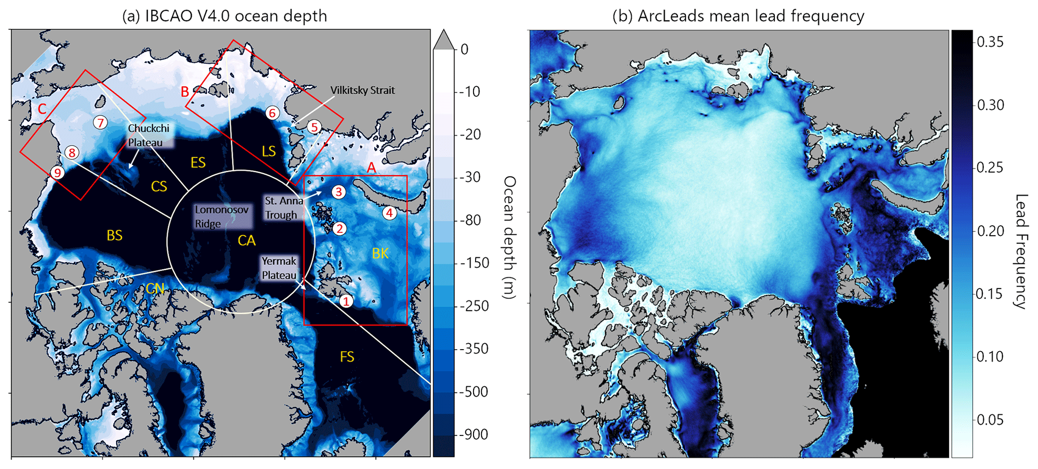
Figure 1(a) IBCAO version 4.0 ocean depth (Jakobsson et al., 2020) and overview of the Arctic Ocean, analyzed sub-regions, and points of interest. Red boxes indicate regions used in Figs. 3, 4 and 5. (b) Pan-Arctic mean sea-ice lead frequencies for the months of November–April in the period 2002/03–2020/21 (Reiser et al., 2020).
2.3 Atmospheric data
Atmospheric data are taken from simulations of the non-hydrostatic regional climate model COnsortium for Small-scale MOdeling – Climate Mode (COSMO-CLM or CCLM; Steger and Bucchignani, 2020). CCLM was adapted to polar regions by implementing a two-layer sea-ice model and new parameterizations for the atmospheric boundary layer (Heinemann et al., 2021). CCLM has been used for several studies of air–sea-ice–ocean interactions and boundary layer processes in polar regions (e.g., Gutjahr et al., 2016; Kohnemann and Heinemann, 2021, Heinemann et al., 2022). CCLM is used with a horizontal resolution of 15 km for the whole Arctic (C15). Initial and boundary data are taken from ERA-Interim reanalyses (Dee et al., 2011). The model is used in a forecast mode with daily re-initialization. Model output is available every 1 h. Sea-ice concentration is taken as daily data from AMSR2 data (Spreen et al., 2008). Sea-ice thickness is prescribed daily from interpolated Pan-Arctic Ice–Ocean Modeling and Assimilation System (PIOMAS) fields (Zhang and Rothrock, 2003). For the present study, monthly averages of wind field data at 10 m are used. C15 data are available for the whole Arctic for 2002–2016. As a second atmospheric dataset, we use ECMWF ERA5 data (Hersbach et al., 2020), which have a horizontal resolution of about 30 km. We here use monthly averages of wind speed, horizontal wind components and wind divergence for the winter months of November to April in the period 2002 to 2021 downloaded from the Copernicus Climate Data Store (https://cds.climate.copernicus.eu/, last access: 10 January 2023).
2.4 Ocean data
Ocean data of the surface current velocity (F_SCV) and eddy kinetic energy (F_EKE) are from simulations of the Finite Element Sea Ice–Ice-Shelf–Ocean Model (FESOM) version 1.4 (Wang et al., 2014). FESOM has previously been used also in other studies for the simulation of ocean currents in the Arctic (e.g., Wang et al., 2016; Wekerle et al., 2017). Here, the same version of FESOM was used as in Sidorenko et al. (2019) but with a different model grid. FESOM runs on a specialized grid with a global horizontal resolution of approximately 1∘, which is refined to 4.5 km in the Arctic and 2 km for the Laptev Sea. Vertically it is structured into 47 layers with a resolution of 10 m in the upper 100 m and increased layer density near the bottom. Depth data are taken from the 1 min version of the RTopo-2 dataset (Schaffer et al., 2016). The model is initialized with temperature and salinity data from the World Ocean Atlas (Levitus et al., 2010), and river runoff is from the Japanese 55-year Reanalysis or JRA55 (Suzuki et al., 2018). On the global scale, FESOM is driven by ERA-Interim reanalyses (Dee et al., 2011) for the period 1987–2016. The model output is available as monthly means, with selected variables being available as daily means. We here use FESOM data for the Arctic for the period 2002–2016.
2.5 Data processing
Based on the method described in Reiser et al. (2020) and the resulting daily binary lead maps we calculate monthly lead frequencies and the absolute mean lead frequency for the months of November to April for the winters of 2002/03 to 2015/16 (short period) and 2002/03 to 2020/21 (long period), respectively. The short period is used to allow for comparison with FESOM and C15 simulation results, which are available only up to April 2016. The long period is computed to make use of the full lead dataset and allow comparisons with ERA5 wind divergence. Two quantities are calculated from the daily binary lead maps. The lead frequency (LFQ) is a temporally integrated quantity that indicates on how many days during a specified period a pixel is found to be covered by a lead, relative to the number of the available clear-sky observations (Willmes and Heinemann, 2016). Thereby we obtain, e.g., monthly, annual and total lead frequencies for the Arctic. Lead fraction area (LFA), in contrast, is a spatially integrated lead quantity that represents the fraction of a specified area that was covered by leads, i.e., the number of lead pixels over the sum of lead and sea-ice pixels. If more than 50 % of the given area is covered by clouds or artifacts (Reiser et al., 2020), the lead fraction is flagged “cloud covered”. The wind divergence from C15 data was calculated from horizontal wind components at 10 m. We also derived shear from the C15 wind data. It is, however, not shown here because no correlation was found between lead dynamics and this parameter. For ERA5, we directly use the provided monthly divergence data for the 10 m wind field. F_SCV is a direct model output of FESOM given as monthly averages. Monthly averaged eddy kinetic energy (F_EKE) is calculated based on the monthly averaged surface velocities following Wekerle et al. (2017).
Figure 1a provides an overview of the Arctic Ocean with IBCAO ocean depth and individual regions, sectors and points of interest for the subsequent description of detailed results and discussion. An overview of the spatial distribution of mean LFQ based on the new lead climatology of Reiser et al. (2020) is given in Fig. 1b. There are several distinct spatial patterns in the observed lead climatology which confirm the findings of Willmes and Heinemann (2016) but with far more detail. Increased lead frequencies with values of up to 0.4 (meaning that the sea ice at this pixel is covered by leads for more than 40 % of the time in the winter period from November to April) are mainly found on the shelves, along the shelf break, and alongside channels and distinct bathymetric features (Fig. 1b). Several lead “hot spots” can be identified by darker shading that were hitherto unknown or at least not described in detail (see Sect. 3.2). The most dominant spatial lead patterns are mainly found in Fram Strait (FS) and in the Barents and Kara seas (BK), thus close to the marginal ice zone where the ice pack becomes less dense due to strong currents in combination with the increased influence of ocean swell and waves (e.g., Pavlova et al., 2014). The lead data shown here indicate, however, that also in the BK region we can spatially distinguish regions with pronounced LFQ that are associated with sea floor channels or ridges. Also, e.g., the northern edge of the Yermak plateau (northwest of Svalbard, point 1 in Fig. 1) shows an increased lead activity as compared to the surroundings, which gives rise to the assumption that mechanical or thermodynamical sea-ice weakening due to ocean current gradients and eddies (with the associated mixing) influences sea-ice dynamics in this region. Similar patterns are also found around Franz-Josef Land (2), in the St. Anna Trough (3) and west of Novaya Zemlya (4). The Beaufort Sea (BS) and its associated gyre are characterized by a significantly increased LFQ (values can exceed 0.3 in some regions) as compared to the central Arctic Ocean, where LFQ can drop down to below 0.05. The Laptev and East Siberian seas (LS, ES) are mostly characterized by the extended fast-ice area and large flaw polynyas. Additionally, the shelf break and several small islands and shoals pop out in Fig. 1b with very high LFQ values (> 0.4 in polynyas and over shoals). In the Chukchi Sea (CS) we also find a distinct spatial pattern in the lead climatology that is obviously influenced by the sea floor.
3.1 Interannual and regional lead variability and trends
The MODIS lead climatology allows for an in-depth overview of wintertime sea-ice dynamics for the last 2 decades. As shown in Fig. 2a, no overall trend is present in pan-Arctic monthly lead fractions (LFA). However, a significant seasonal and interannual variability can be noted with the tendency of a generally lower lead fraction at the end of winter (April) with frequency values of 0.1 on average compared to 0.15 in November. This is a reasonable finding considering that the ice becomes thicker, more compact and thus less mobile throughout the winter months. Figure 2b–i show the interannual and seasonal variability in lead fractions for individual regions (see map in Fig. 2a). None of the presented regions exhibits a significant trend if the entire winter season is considered (November–April).
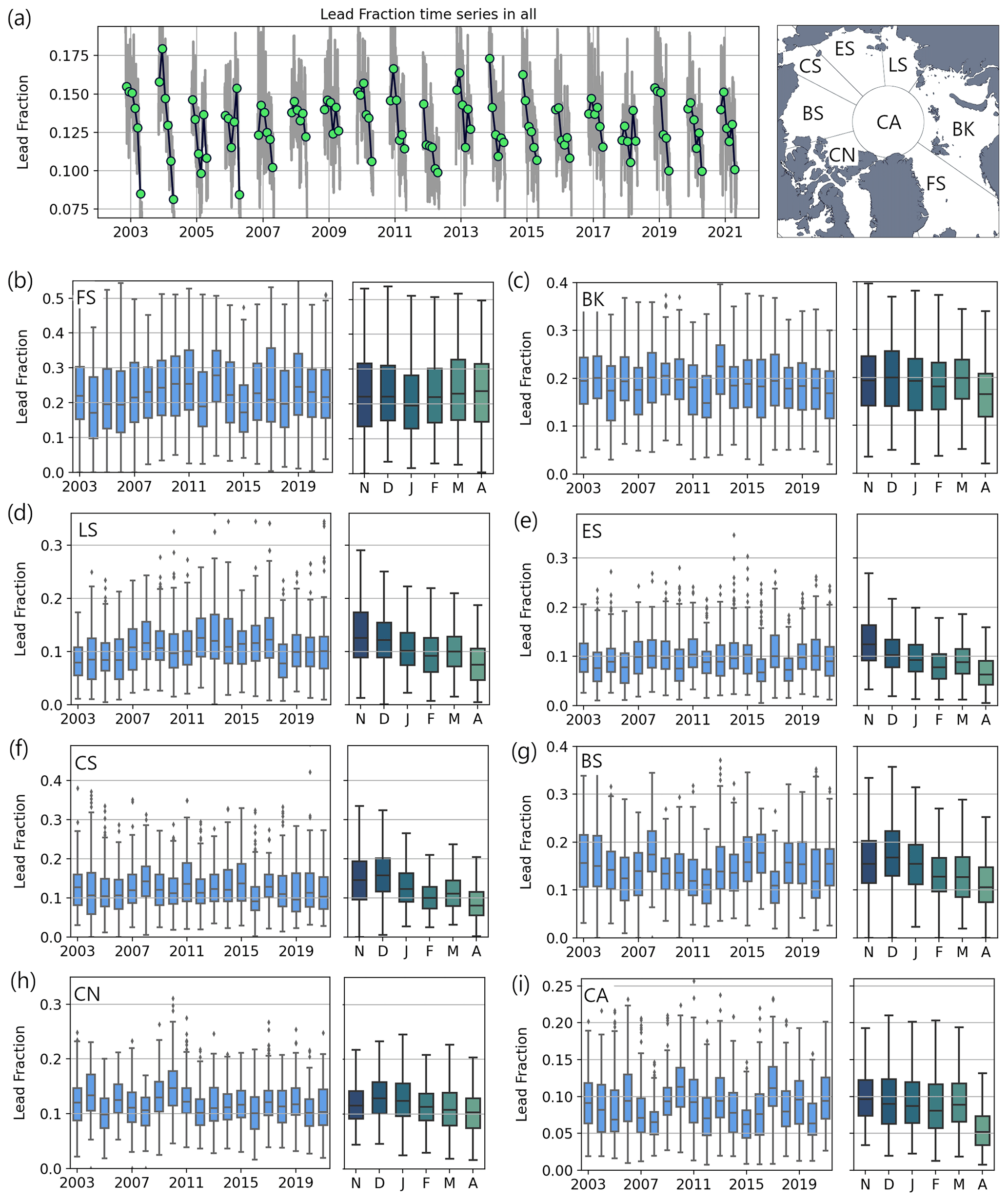
Figure 2(a) Time series of daily (grey) and monthly (green) Arctic lead fractions for all areas: inset map indicates individual regions. (b–f) Lead fractions for individual regions throughout years and months for regions indicated in inset map: Fram Strait (FS), Barents and Kara seas (BK), Laptev Sea (LS), East Siberian Sea (ES), Chukchi Sea (CS), Beaufort Sea (BS), Canadian Arctic (CN), and central Arctic (CA). The given spread per year represents the distribution of daily lead fractions per region and winter. Left panels: box–whisker plots for individual years with the median, the 25th and 75th percentiles as boxes, and the 10th and 90th percentiles as error bars. Right panels: like left panels but for individual months.
The magnitude of LFA differs between regions with the largest area covered by leads found in the FS sector (> 0.5, note the different scales for individual regions). A strong seasonal variability is present in all regions, which is also indicated by the seasonal evolution of lead fractions per region (right panel for each region). While the change in area covered by leads is less pronounced in the FS, Canadian Arctic (CN) and BK sectors throughout winter, all other regions are characterized by a continuous decrease in lead fractions from November to April. In the central Arctic (CA) lead fractions are the lowest (< 0.1 on average) and rather stable from November to March, but a significant drop is present from March to April, when lead fraction here is on average only around 0.05. Outliers in monthly lead fractions in all sectors indicate that strong anomalies are found only on the monthly scale, while there is no full year with extremely anomalous lead fractions on the pan-Arctic and the regional scales. This finding is presented in more detail in latitude-averaged monthly LFQ anomalies in 5∘ longitude bins for November 2002 to April 2021.
Figure 3a shows the temporal evolution of LFQ anomalies in sea-ice regions between 70 and 90∘ N across longitudes in the Arctic Ocean (the coastlines below the figure indicate the respective position across longitudes). Significant trends are not identified. The most interesting feature here is an indication of strong lead events that are expressed through strong positive anomalies (red dots). Several of these events can be identified from the diagram across all longitudes, while the Siberian sector of the Arctic (90–180∘ E) generally shows less monthly variability as compared to other sectors. Two events are exemplarily extracted and shown as monthly lead anomaly maps.
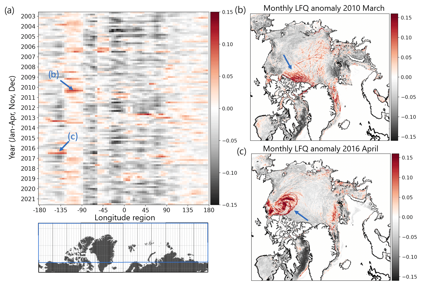
Figure 3(a) Latitude-averaged (70–90∘ N) monthly LFQ anomalies in 5∘ longitude bins for November 2002 to April 2021. Only the months of November, December, January, February, March and April are shown. (b) Monthly lead frequency (LFQ) anomaly for March 2010, with a very strong positive lead anomaly north of the Canadian Archipelago and (c) monthly LFQ anomaly for April 2016, underpinning the strong positive lead anomaly in the Beaufort Sea that is also given in the overview in (a). Anomalies are calculated relative to the climatological monthly means.
In Fig. 3b, the monthly LFQ map shows strong anomalies north of the Canadian Archipelago with values of up to 15 % above average (see marker b for comparison in Fig. 3a). An extreme lead event in the Beaufort Sea in April 2016 with similar anomalies is shown in Fig. 3c (marker c in Fig. 3a), which resulted from a series of preceding events that preconditioned the ice in the Beaufort Sea to become weaker and thinner (Babb et al., 2019). The event from 2013 in the Beaufort Sea discussed in Rheinlænder et al. (2022) is also visible in Fig. 3.
The question of trends in wintertime lead dynamics has been addressed in several studies so far. For example, Wang et al. (2016) did not observe significant lead trends in the Arctic, and Lewis and Hutchings (2019) reported no significant trend in the total number of days with leads per winter season. Qu et al. (2021) discuss a positive interannual trend in the April lead area of the Beaufort Sea and close relation to enhanced ice motion driven by an enhanced Beaufort High and persistent easterly winds. Significant interannual trends cannot be found in our annual time series for this region (Fig. 2g). Also for individual months, no significant trends can be found at the 5 % significance level.
3.2 Sea-ice leads, bathymetry and ocean currents
The mean spatial lead patterns presented in Fig. 1b can be compared with FESOM simulations of ocean surface current velocities and EKE to evaluate a potential role of the ocean in shaping the presented observations (Fig. 4a, b). One can see that higher values in both FESOM variables in many places occur with increased lead frequencies. This agreement is noteworthy especially because the two datasets are independent of one another (observations and simulation). The F_SCV clearly shows what is usually referred to as the Arctic Boundary Current (Aksenov et al., 2011) with branches crossing the channels of the Barents and Kara seas and entering the Laptev Sea via the Vilkitsky Strait (5). Some of the spatial structures exhibited by these current branches resemble the lead patterns, for example, along the shelf break north of Svalbard, at the eastern edge of St. Anna Trough, in Vilkitsky Strait or in the northern Chukchi Sea, which gives rise to the hypothesis that ocean currents are an important driver for the mean susceptibility of sea-ice lead occurrence. While increased current speeds are mostly associated with high F_EKE values, the latter are more tied to bathymetric features and ocean depths above −1000 m.
A more detailed perspective on the relation of lead frequencies, ocean depth and ocean currents is presented in Figs. 5, 6 and 7 for three different sub-regions and transects. These regions were selected because bathymetry is highly variable here, and a lot of details can be found in the patterns of LFQ, F_SCV and F_EKE.
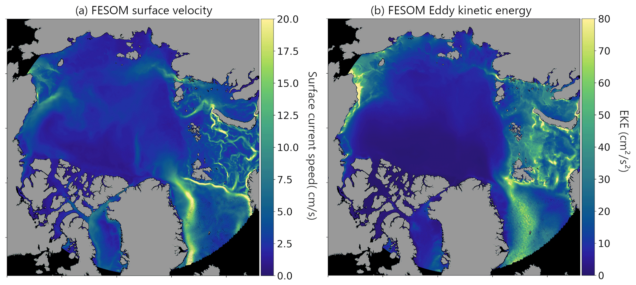
Figure 4(a) FESOM ocean surface current velocity (F_SCV) and (b) FESOM eddy kinetic energy (F_EKE) for November–April 2002/03–2015/16.
3.2.1 Barents and Kara seas
In Fig. 5a, we show mean LFQ, IBCAO ocean depth, mean F_SCV and mean F_EKE in the Barents Sea (see red box around BK in Fig. 1a). The spatial overview reveals the above-mentioned patterns in more detail. In many places high LFQ values are associated with strong bathymetric gradients, increased current speeds and high F_EKE. Ocean depth in the Barents Sea ranges between −400 and −100 m in the presented subset and is characterized by several elevations and channels with outlets towards the shelf break north of Svalbard (point 1) and Franz-Josef Land (2), where ocean depth drops immediately to less than −1000 m. The eastern slope of St. Anna Trough (3) shows moreover a branch of significantly increased current speeds and a band of LFQ values above 0.4, which means that the sea ice in this region is covered by leads for more than 40 % of the time in the winter period from November to April. The highlighted transect (red) allows for a more detailed comparison in Fig. 5e and f. Reaching from northwest to southeast through the Barents Sea, the LFQ transect exhibits local maxima right above the indicated seafloor elevations, which reach from about −350 up to −100 m in this region (Fig. 5e). At the northwestern coast of Novaya Zemlya the LFQ maximum is found over the slope rather than on top of the shelf (4). At this position the LFQ maximum is neighbored by strong maxima of F_SCV and F_EKE by the FESOM model (Fig. 5f). The other seafloor elevations along the presented transect (e.g., at 69, 207, 345 km) do not present F_SCV or F_EKE maxima like LFQ.
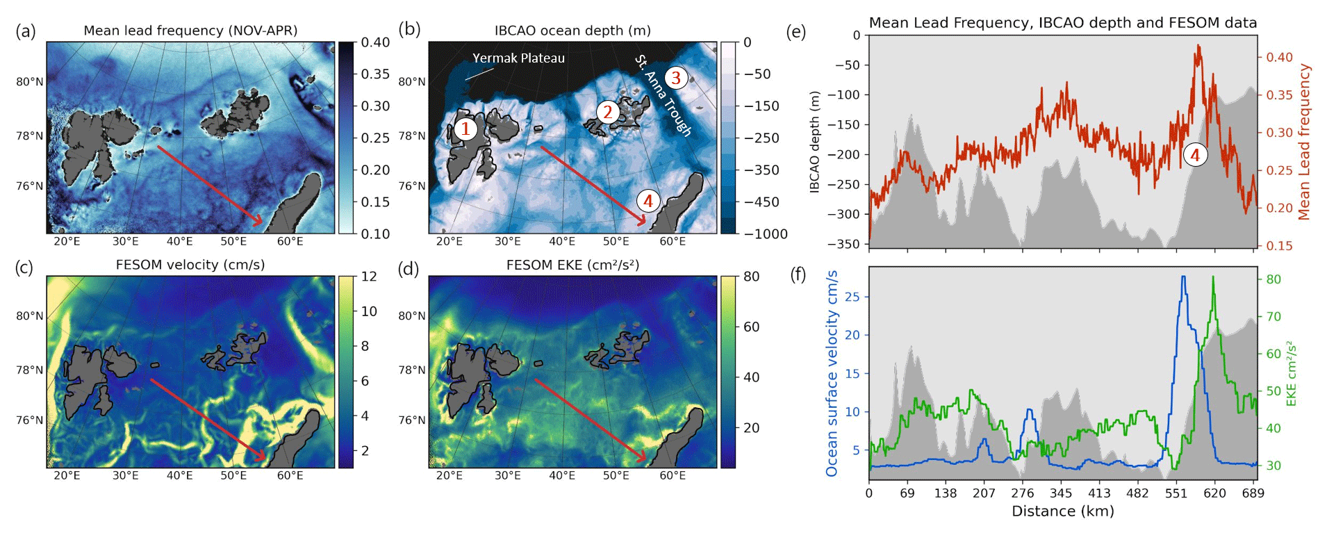
Figure 5(a) Mean wintertime lead frequency for 2002–2016, (b) IBCAO ocean depth (Jakobsson et al., 2020), (c) mean FESOM surface current velocity (F_SCV) and (d) mean FESOM EKE (F_EKE) in the Barents Sea. Transect (red line) values: (e) mean lead frequency (red) and ocean depth and (f) FESOM current velocity (F_SCV, blue) and FESOM EKE (F_EKE, green); see red box A in Fig. 1a.
3.2.2 Laptev Sea
Similar features are found in a close-up for the Laptev Sea (Fig. 6, see red box around LS in Fig. 1a). Most prominent here are the flaw polynyas and the extended fast-ice area, which are characterized by high and low lead activity, respectively. But increased LFQ values are also found in the outflow region of Vilkitsky Strait (5), between the Taymyr Peninsula and Bolshevik Island, and along the shelf break (6). The chosen transect crosses Vilkitsky Strait up to the shelf and continues over the shelf break towards the deep ocean. Here, increased LFQ is found at the start of the transect southeast of Bolshevik Island where a flaw polynya is found, at the southern slope of Vilkitsky Trough and over the shelf break (Fig. 6e). Except for the flaw polynya, we find the mentioned LFQ maxima to be associated with maxima in both F_SCV and F_EKE. Local maxima for both parameters are found on the slope of Vilkitsky canyon, as well as over the shelf break, indicating that the ocean plays a crucial role in shaping the sea-ice stability in this region. The importance of the Vilkitsky canyon in transporting water masses was documented in several studies (e.g., Harms and Karcher, 2005) with the general surface circulation in the Laptev Sea being characterized by an eastward flow that causes an inflow of saline water masses from Vilkitsky Strait (Janout et al., 2020). While the inflow itself does not explain increased lead frequencies in this region and over the shelf break, intensified currents and tide-induced shear (Janout et al., 2015; Janout and Lenn, 2014) might be a driver for frequent sea-ice break-up. Thus, changing water masses and strong surface gradients in Vilkitsky Strait and over the Laptev Sea shelf break potentially represent favorable conditions for the formation of leads. The overall lead patterns in the Atlantic and Siberian sectors of the Arctic Ocean with increased lead frequencies over seafloor channels, over ridges and along the shelf break might therefore be related to the structure and pathway of the Arctic Circumpolar Boundary Current (Pnyushkov et al., 2015, Aksenov et al., 2011).
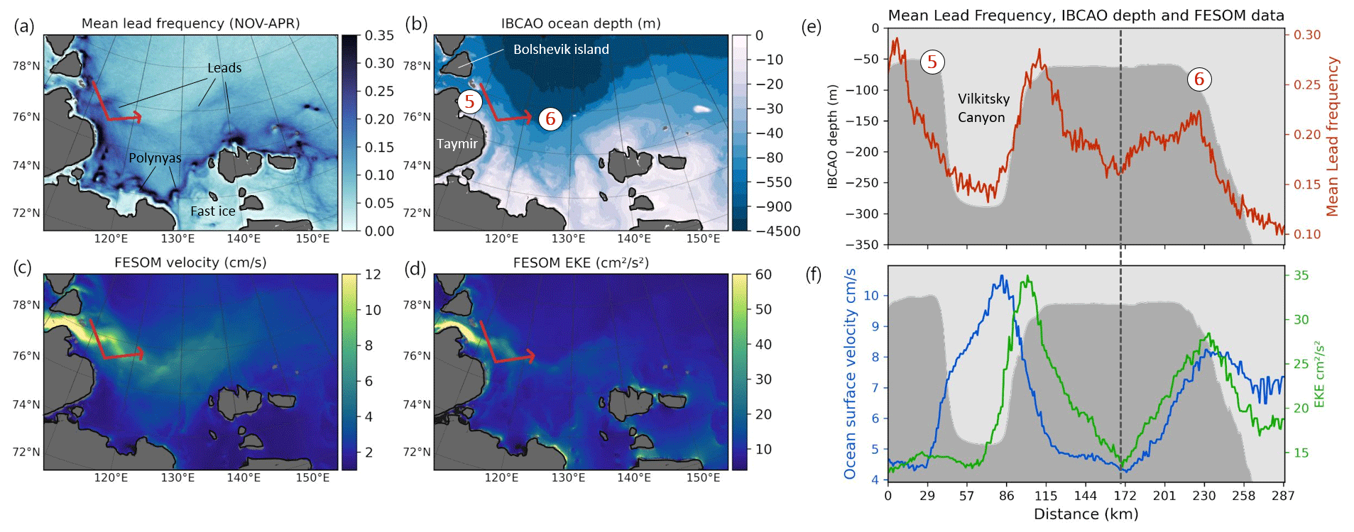
Figure 6As in Fig. 5 but for the Laptev Sea; see red box B in Fig. 1a.
3.2.3 Chukchi Sea
In the Chukchi Sea (Fig. 7, see red box around CS in Fig. 1a) and around Wrangel Island we find some point-shaped areas of high LFQ and a linear band of slightly increased LFQ reaching from the northeastern edge of Bering Strait towards the northwest. The IBCAO subset indicates that the latter pattern is associated with a shallow channel in this region, i.e., Herald Canyon (7), and the southwestern slope of Herald Shoal (8), while the point-like LFQ maxima are found north of Point Barrow (9), over Hanna Shoal (10) and next to a small island east of Wrangel. The ocean current velocities show two branches of increased speed reaching up north alongside Herald Shoal. F_EKE values are increased next to the coast and also in the band of increased LFQ on the western side of Herald Shoal. The profile in this subset crosses Herald Canyon, continues over Herald Shoal and ends in the central channel of the Chukchi Sea. It indicates the strongly increased LFQ on the southwestern slope of Herald Shoal that is part of the band of higher LFQs mentioned above and with a pronounced peak right over Herald Shoal (Fig. 7e). The latter is accompanied by increased F_EKE in the ocean data, while the LFQ peak at the slope shows maxima for both F_SCV and F_EKE (Fig. 7f). Towards the central channel, LFQ, F_SCV and F_EKE increase coincidently. The indicated lead patterns can be attributed to the general circulation in the Chukchi Sea, which is characterized by a broad northeasterly flow following the topography with some regions of intensified currents, e.g., in Herald Canyon (Winsor and Chapman, 2004; Stabeno et al., 2018).
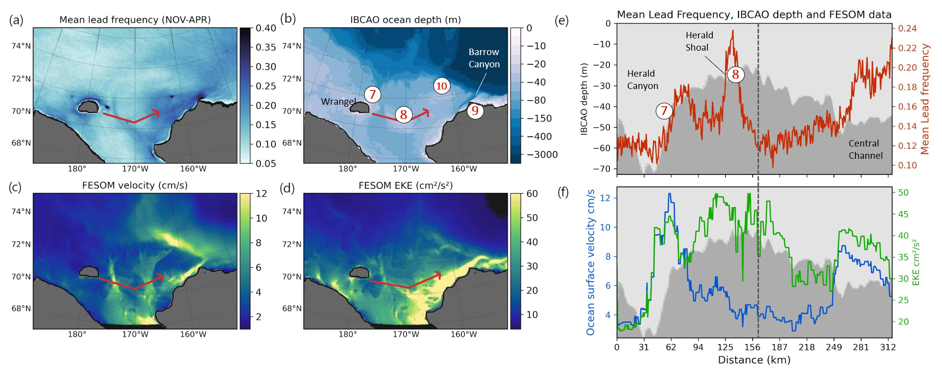
Figure 7As in Fig. 5 but for the Chukchi Sea; see red box C in Fig. 1a.
3.2.4 Overall influence of surface currents and EKE
In order to pinpoint the Arctic regions where the ocean (F_SCV and F_EKE) has the largest influence on the observed lead frequencies, we calculated what we refer to as the coincident percentile exceedance (CPE), which is the percentile value that is exceeded in both datasets (LFQ and F_SCV or LFQ and F_EKE) at a certain position (Fig. 8). This metric allows us to identify the regions in which there is an indication that the ocean is a driver for lead dynamics. The resulting map shows distinct patterns with CPE values over 90 in several regions (i.e., values are above the 90th percentile in both datasets). The most dominant are the Fram Strait, the Barents and Kara seas, and the coast of Alaska, north of Point Barrow. Several bathymetric features can be recognized in both maps, e.g., Herald Canyon in the Chukchi Sea, the Vilkitsky Canyon in the western Laptev Sea and the slope of St. Anna Trough in the Kara Sea. In Fram Strait, we find high CPE for LFQ and F_SCV in a broad band between Greenland and Svalbard (Fig. 8a), while the influence of F_EKE on leads seems to be limited to the marginal ice zone. In the Barents Sea we find individual current branches that are associated with high LFQ values. Many more interesting details can be seen in the two maps in Fig. 8 that provide insight into how F_SCV and F_EKE affect the long-term lead dynamics individually and in which regions the stability of sea ice seems to be more prone to processes in the ocean. This documented effect of the ocean on sea-ice lead dynamics is most obvious in the long-term, i.e., in the climatology.
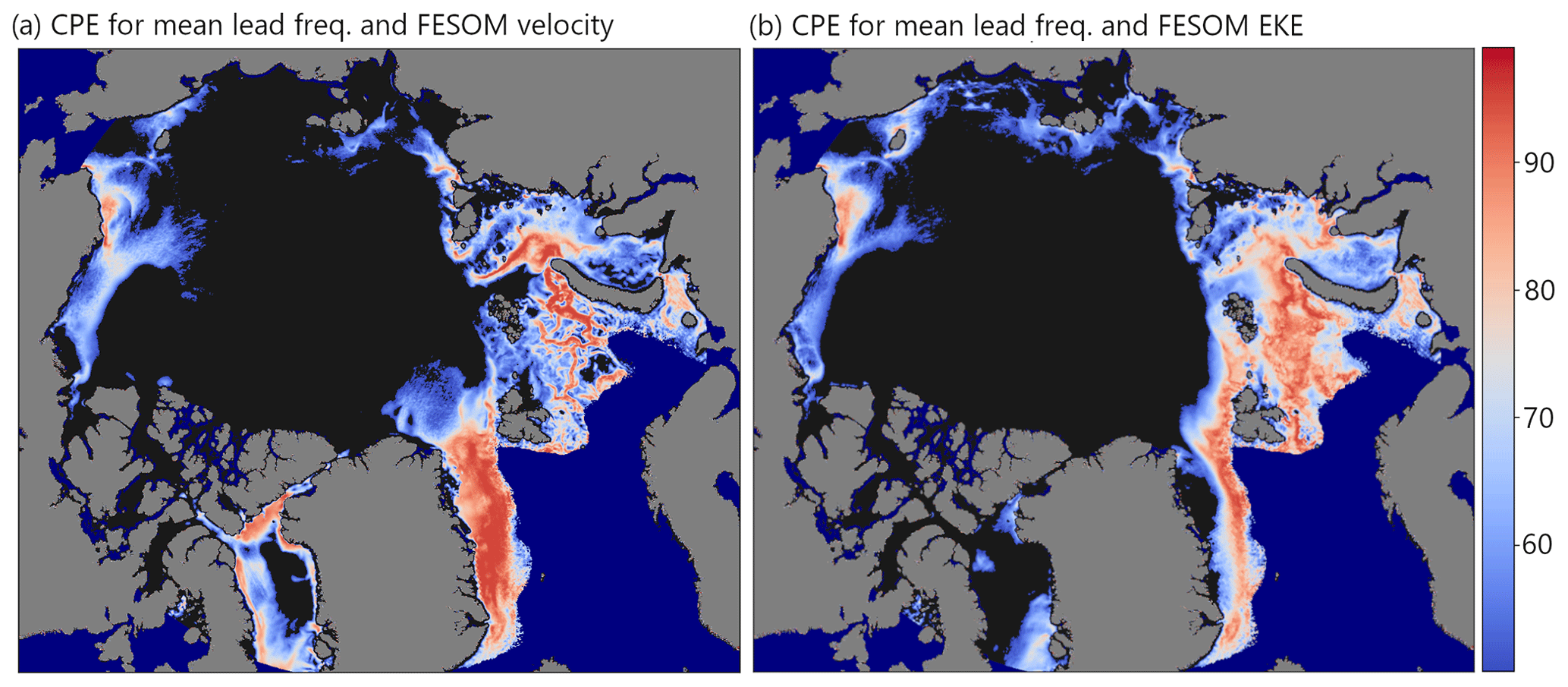
Figure 8The coincident percentile exceedance (CPE) for the mean wintertime lead frequency for 2002–2016 and (a) FESOM surface current velocity (F_SCV) and (b) FESOM EKE (F_EKE). Values indicate the value percentile per pixel that exceeds coincidently in both datasets and are cut off at values below the 50th percentile (black areas).
3.2.5 Spatial lead patterns and winds
To understand the role of winds in driving the observed patterns in lead formation we look at wind components and derived mean quantities. The average wind speed and shear (not shown) provide no indication for driving the observed spatial patterns in the lead climatology on a pan-Arctic scale. This also holds when daily instead of monthly wind data are considered. However, the mean wind divergence (Fig. 9) shows a dominant region of positive divergence centered around the Beaufort Gyre. This divergence pattern with maxima especially in the southern Beaufort Sea is well aligned with the Beaufort Sea LFQ maximum indicated in Fig. 1b. This broad region of generally increased lead occurrences might therefore be influenced by the mean divergence of the wind field rather than by ocean currents. Also, Fram Strait is characterized by a positive wind divergence in the long-term mean that can consequently add up to the influence of enhanced ocean currents on average lead frequencies in this region. In general, however, winds seem to have a larger effect on the temporal dynamics of leads rather than on the mean spatial patterns. This will be presented in detail in Sect. 3.3.
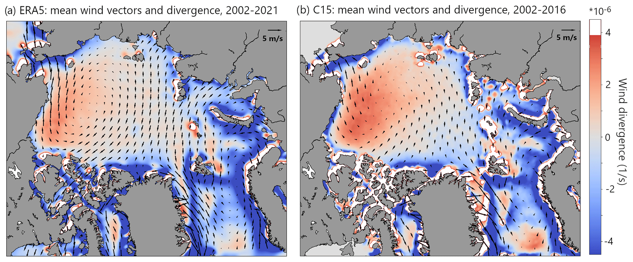
Figure 9Spatial fields of mean wind divergence (in 10−6 s−1) and mean horizontal wind vectors for (a) ERA5 for 2002–2021 (Hersbach et al., 2020) and (b) C15 for 2002–2016 for November to April. Wind vectors are shown with a spatial distance of 15 grid points for ERA5 and 10 grid points for C15 (wind vector scale in the upper right corner). Regions with values exceeding s−1 are masked out (white areas), since they are influenced by the transition of land to ocean in coastal areas and different resolutions of the associated land masks in most cases.
3.2.6 Winds vs. ocean forcing in the mean lead fields
As shown above, the spatial patterns in the lead climatology show a strong coincidence with the spatial patterns of maxima in ocean surface currents and EKE. A link to mean winds can only be found in the fields of mean wind divergence and is constrained to the Beaufort Sea and Fram Strait. FESOM allows us to distinguish between local forcing provided by winds and ocean individually in terms of sea-ice surface and sea-ice bottom stress. The FESOM stress difference (bottom stress−top stress) is given in Fig. 10a. Here, we can see that the modeled stress fields show the highest difference (with sea-ice bottom stress exceeding sea-ice surface stress) right where the observed lead frequencies are characterized by their most dominant patterns, i.e., the shelf break north of Franz-Josef Land, the eastern slop of St. Anna Trough, Vilkitsky Strait and the western part of the Laptev Sea shelf break, as well as Herald Canyon in the Chukchi Sea. The regions where the stress difference is positive (ocean dominates) are coincident with high lead frequencies and are highlighted in Fig. 10b, which in comparison with Fig. 8 provides evidence for where the ocean plays a dominant role in shaping the mean lead patterns in the observed lead climatology. The region north and east of Point Barrow with its high mean lead frequencies is apparently characterized by a mixture of ocean and wind stress dominating here, while bathymetry and coastal geometry seem to act as two factors for lead opening/closing dynamics superimposed to one another. While the role of atmospheric forcing here was thoroughly analyzed and presented recently, e.g., by Jewell et al. (2023), the influence of ocean processes and bathymetry requires additional research. Untangling individual regional forcings for lead dynamics will generally need an in-depth analysis that includes mechanistic explanations of dynamics, thermodynamics and the influence of coastal geometry.
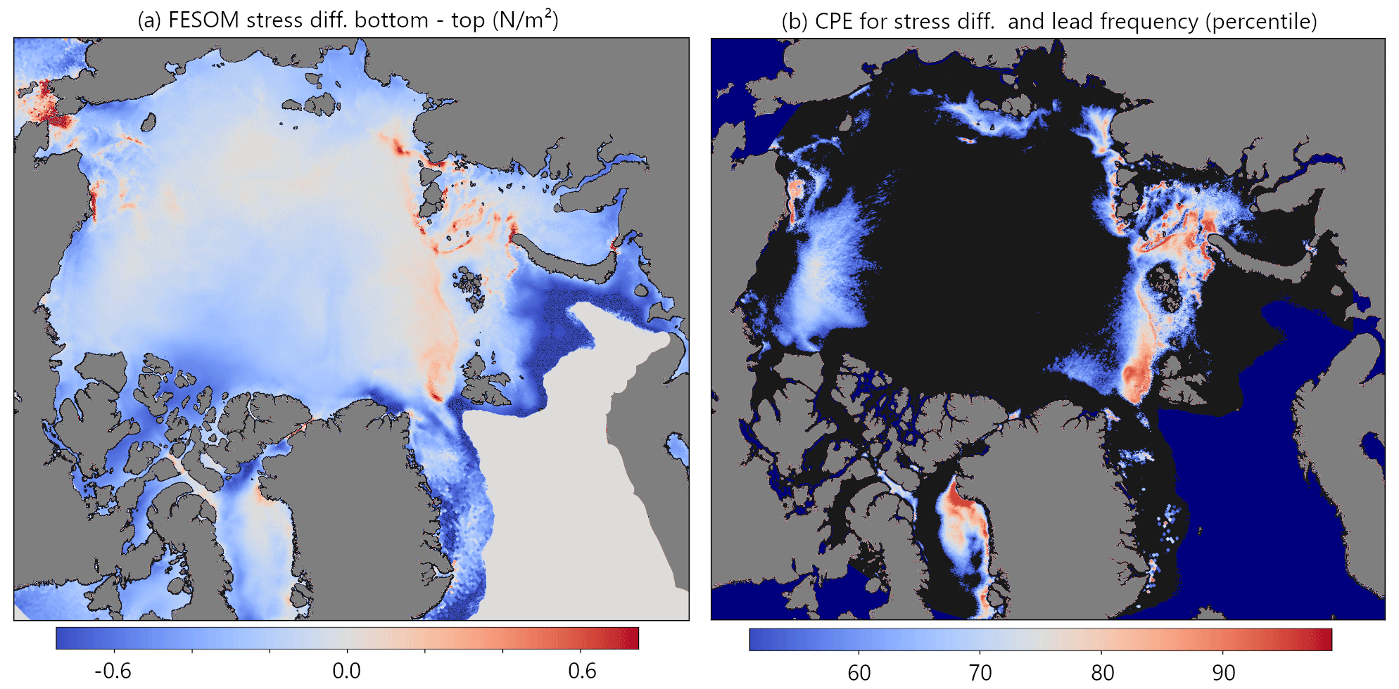
Figure 10(a) FESOM sea-ice stress difference (bottom−top). (b) Coincident percentile exceedance (CPE) of the FESOM stress difference and mean lead frequency.
3.3 Sea-ice leads and wind and temporal variability
To get a better insight into the driving mechanism for the temporal lead variability discussed above we investigate the grid-point correlation of monthly LFQ with wind from ERA5 and C15 model data. No significant correlations are found for the wind speed and wind shear (not shown). The Pearson correlation coefficient for monthly LFQ with wind divergence is shown in Fig. 11 for ERA5 and C15. The latter is only available for the period 2002–2016. Only significant sectors are considered in both maps (p values <0.05). There are clearly two main regions where a significant correlation between wind divergence and lead dynamics can be identified: in both the Beaufort Sea and Fram Strait, the variability in monthly wind divergence correlates with the mean monthly lead frequency. While the correlation coefficient is generally only in the range between 0.5 and 0.7, the clustering of values in the two mentioned regions indicates that wind divergence is a significant driver of lead dynamics here. For the C15 data, there is a maximum correlation in the approximate center of the Beaufort Gyre (Fig. 11b), while this is less pronounced with ERA5 data (Fig. 11a). Towards Fram Strait, correlations increase southward.
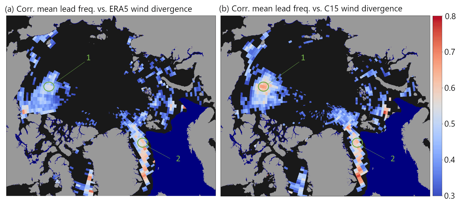
Figure 11Pearson correlation for monthly values of mean lead frequency and monthly mean wind divergence from (a) ERA5 (Hersbach et al., 2020) for 2002–2020 (November–April) and (b) C15 for 2002–2016 (November–April). Coefficients are only shown for p values <0.05.
No significant correlation is found in the central and Siberian Arctic, suggesting that on average winds play only a minor role in the regional lead dynamics for these sectors. The Barents and Kara seas indicate some sectors with a significant correlation and with a maximum at the ice edge. Two points are indicated (1: central Beaufort Sea; 2: Fram Strait) from where time series are extracted to show the temporal evolution of monthly values of LFQ and wind divergence from ERA5 and C15. Figure 12 shows the evolution of monthly averages of these data at points 1 and 2 in Fig. 11 for November to April from 2002–2021 (ERA5) and 2002–2016 (C15). The comparison of time series suggests that peaks in the mean LFQ (grey) are very often accompanied by high average wind divergence (blue and orange). This is also confirmed by the associated scatterplots on the right-hand side of the time series panels, where a positive correlation between wind divergence and LFQ is indicated for both ERA5 and C15 data, respectively. In point 1 (Beaufort Sea), the correlation coefficient is 0.67 for LFQ with C15 data and 0.54 for LFQ with ERA5 data. In point 2 (Fram Strait) these values are 0.69 and 0.61, respectively (note that p values for all colored points in Fig. 12 are < 0.05). Figure 9 puts this in context with the fields of mean divergence and mean horizontal wind vectors from ERA5 and C15 datasets. If the coastal regions are not considered (where the effects due to friction and topography dominate), the main maximum in mean wind divergence is found in the Beaufort Sea. This maximum is associated with the mean anticyclonic circulation of the Beaufort high and is more pronounced in the C15 data. The mean wind vector fields reflect also the Transpolar Drift from the Laptev Sea to Fram Strait and the southward winds with high directional constancy over Fram Strait.
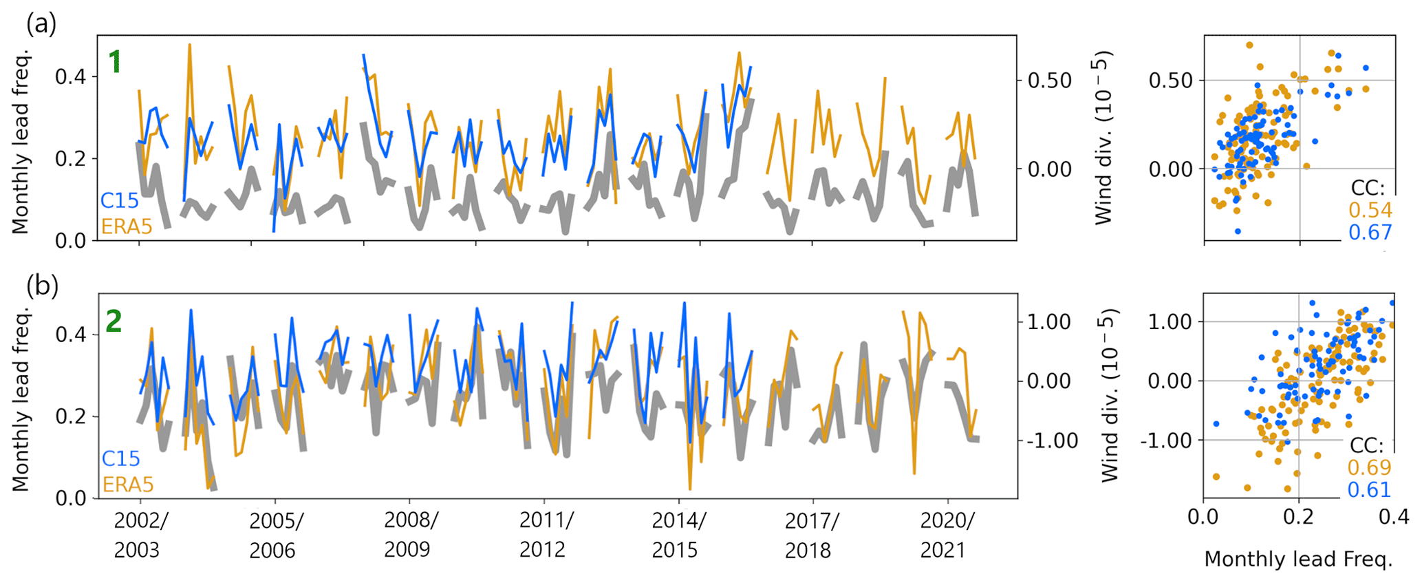
Figure 12Time series of monthly and sectoral averages of lead frequency (grey) and wind divergence from ERA5 (Hersbach et al., 2020; orange) and C15 (blue), as well as associated scatterplots for (a) point 1 and (b) point 2 in Fig. 11. Correlation coefficients are indicated in the scatterplots for LFQ with ERA5 (orange) and C15 (blue).
With the perspective of a changing Arctic, knowledge about the drivers of wintertime sea-ice dynamics is key. In this context, insight about where and when leads are forming and an overview about the conditions that favor the formation of leads are essential. When extreme sea-ice break-up events are observed, the focus is most often set on explaining the driving mechanisms (Rheinlænder et al., 2022; Babb et al., 2019), which are generally strong winds or (in the marginal ice zone) waves (e.g., Pavlova et al., 2014). Also in some studies, the attribution of overall anthropogenic influences on extreme events in Arctic sea ice is analyzed (Kirchmeier-Young et al., 2017). In any case, the drivers for sea-ice dynamics on seasonal and interannual timescales are found in ocean processes and in the atmosphere. However, the relative importance of oceanic and atmospheric processes for changes in the Arctic sea-ice cover is not well established (Liu et al., 2022). In this study, we therefore present a first attempt to describe and untangle the influence of both drivers spatially and temporally. The drift of sea ice and the associated stress is directly connected to the formation of leads. The main circulation patterns of Arctic sea ice, the Beaufort Gyre and the Transpolar Drift, have shown a net strengthening during the last decades, which was attributed mainly to a reduced multiyear sea-ice cover (Kwok et al., 2013, Stroeve and Notz, 2018). Younger and thinner ice is expected to be more prone to break-up and lead formation (Zhang et al., 2012). However, we could not observe pan-Arctic trends in wintertime lead fractions in the period between 2002 and 2021 (see Fig. 2). The trends in detected leads can be biased by overlying trends in cloud frequencies. This effect is, however, compensated for in our trend calculation. A small positive lead area trend of 3700 km2 yr−1 was reported by Hoffman et al. (2022), however, with a large uncertainty and based on a different lead climatology, which shows less of the patterns highlighted in this study. Eicken et al. (2012) describe an increase in lead frequency in the Beaufort Sea in the period of 2004–2010 in comparison to 1993–2004. They explain this finding with less multiyear ice and increased divergence (Hutchings and Rigor, 2012; Babb et al., 2022). From the data we present here, an increase in lead frequencies in the Beaufort Sea cannot be inferred, but as our analysis does not include lead observations before 2002, no conclusion can be drawn about changes in comparison to the period prior to this year. In Lewis and Hutchings (2019), no trend in the occurrence of leads in the Beaufort Sea is found over 20 winters from December 1993 to May 2013.
4.1 Winds and leads
The role of storms and waves on wintertime sea-ice break-up is well known (e.g., Graham et al., 2019). We could, however, not find an overall correlation between leads and wind speed in long-term data, although their relation is well documented for several case studies, at least for shorter timescales and extreme events (e.g., Rheinlænder et al., 2022). Instead, we find the wind divergence to be a dominant driver for large-scale lead dynamics and sea-ice variability. We therefore assume the influence of wind speed on large-scale lead formation to be confined to short timescales and divergent conditions, at least for cases when the ice cover is still dense and compact. On the other hand, increasing wind speeds are projected for the future wintertime Arctic in conditions with a less dense sea-ice cover and consequently surface warming (Mioduszewski et al., 2018). Thus, a potentially enhanced sea-ice loss and increasing lead fractions can be amplified by the resulting intensified winds in the future. In the Barents and Kara seas with their marginal ice zones we find generally high lead frequencies. Here, the influence of winds affects the redistribution of sea ice and thereby the formation of leads (Pavlova et al., 2014). From the ocean side, the advection of heat through winds can trigger a thermodynamic weakening of the sea-ice cover, which can favor a break-up in regions of strong surface gradients. We find high lead frequencies also in Fram Strait, where ice export is directly connected to higher southward ice drift velocities due to stronger geostrophic winds (Smedsrud et al., 2011). Our findings show that here also the enhanced lead activity can be attributed to strong ocean surface currents (in the climatology) and to wind divergence on seasonal scales (Figs. 6 and 10). In the Beaufort Sea, we find a large region of enhanced lead activity around the Beaufort Gyre that shows significant correlation with wind divergence. High sea-ice divergence in this region is reported also by Wang et al. (2016) based on FESOM simulations with 4.5 km horizontal resolution in the Arctic and by Spreen et al. (2017) based on RADARSAT satellite data. The finding that changes in sea-ice coverage in the Beaufort Sea are primarily wind driven was also reported by Frey et al. (2015). While the correlation of changes in sectoral monthly LFQ anomalies with monthly wind data shows significance only for wind divergence in the given regions in this analysis (Fig. 11), we have to make clear that an in-depth analysis of winds and leads will potentially offer a more detailed insight. In this context, the lower spatial resolution of the atmospheric data (15 and 30 km, for C15 and ERA5, respectively) in comparison to FESOM (up to 4.5 km) needs to be mentioned as a potential factor for blurring fine-scale variabilities. In individual regions and for certain periods and events, strong wind speeds and thin ice (Jewell and Hutchings, 2023), as well as the location and trajectory of pressure systems (e.g., Aue et al., 2022) and the effect of coastal geometry (Lewis and Hutchings, 2019), will definitely play a significant role in the opening and closing of leads. Only recently, Jewell et al. (2023) have demonstrated how coastal boundaries modify the response of sea-ice dynamics to wind forcing. Generally speaking, it will require an in-depth analysis that includes mechanistic explanations of dynamics, thermodynamics and the influence of coastal geometry to be able to identify individual regional forcings for lead dynamics (e.g., Jewell et al., 2023; Rheinlænder et al., 2022; Babb et al., 2019).
4.2 Ocean and leads
The spatial patterns in mean lead frequencies (Fig. 1b) seem to be significantly affected by ocean bathymetry and the Arctic Circumpolar Boundary Current (Aksenov et al., 2011; Pnyushkov et al., 2015), especially with its Barents Sea branch and its pathways along the shelf break. While we can assume that it is not the heat of the Atlantic water directly that triggers increased sea-ice break-up, it might well be intensified currents and tide-induced shear (Janout et al., 2015; Årthun et al., 2019). Tides are not included in the FESOM simulations, which means that the contribution of this component could even enhance the suggested governing role of the ocean on preconditioning the sea-ice stability. Holloway and Proshutinsky (2007) show that tides are capable of enhancing the loss of heat from Atlantic waters. The impact of tide-driven mixing on sea ice is characterized by an enhanced ocean heat flux that causes a general sea-ice thinning and thereby makes the ice more prone to lead formation. This suggests the hypothesis that some of the lead patterns that can be seen in Fig. 1b are due to so-called tidal leads. This cannot, however, be answered with the presented analysis. The fine details in the spatial lead patterns that can be seen in our lead climatology (see Figs. 5, 6, 7) probably have the potential to reveal much more of what is happening in the ocean and about the pathways and branches of water masses that could hitherto only be described with model and mooring data.
For the eastern Arctic Ocean, i.e., the Laptev Sea and northern Kara Sea, an increased oceanic heat flux from intermediate-depth warm Atlantic water to the surface mixed layer and sea ice was reported by Polyakov et al. (2020). Such a warming at the ocean surface has the potential for a thermodynamic weakening of sea ice in these regions, which can add up to a potential dynamic weakening through changing water masses and strong surface gradients. Consequently, lead fractions are likely to increase here when increased oceanic heat fluxes persist. In the Chukchi Sea, the ocean currents and branches described by, e.g., Stabeno et al. (2018) clearly resemble the observed spatial lead patterns. Herald Canyon, Barrow Canyon, and Herald and Hanna shoals are the main bathymetric features in this region that govern the ocean currents. We argue here that surface gradients and eddy kinetic energies in these regions are responsible for a frequent formation of sea-ice leads at or next to these structures. The interaction between ocean and leads occurs in two ways. As suggested here, the ocean acts as a preconditioner for sea-ice break-up, and the resulting leads will in turn affect ocean stratification through new ice formation and eddy formation with an associated horizontal redistribution of salinity anomalies (Cohanim et al., 2021). Recently, interactions between ocean–ice heat fluxes, sea-ice cover and upper-ocean eddies were discussed and highlighted as a missing feedback in current climate models (Manucharyan and Thompson, 2022), and Cassianides et al. (2023) suggest that pan-Arctic variations in kinetic and potential energy in the ocean can drive the variability in sea-ice conditions rather than the other way around.
4.3 Overall lead patterns and seasonal impacts
The presented lead climatology shows a lot of very interesting regional details that could not all be described and analyzed in this paper. Especially over the shelf of the Barents and Kara seas, as well as in the East Siberian and Chukchi seas, very distinct but small-scale spatial patterns of mean lead frequencies indicate a significant preconditioning of the ice cover through the ocean and a strong role of bathymetry. These features deserve a thorough in-depth analysis to get a more detailed insight into how the ocean shapes the sea ice and into how projected anomalies of ocean processes in the future could affect the sea-ice cover. It is also suggested that summer sea ice might be affected by deformation events of winter sea ice and the resulting fracturing (Korosov et al., 2022; Hwang et al., 2017). With the presented results we argue that seasonal lead dynamics are mainly driven by winds (e.g., Liu et al., 2022) with the wind divergence yielding the most significant correlations with temporal lead dynamics. The ocean, however, is highly responsible for preconditioning the ice cover and making it more prone in some regions to thinning and break-up than in others with a distinct influence of bathymetry.
We here present a first interpretation of the drivers for the spatial and temporal patterns of Arctic sea-ice leads based on a 20-year climatology from satellite observations with a 1 km2 spatial resolution. No long-term trends can be identified for pan-Arctic average wintertime sea-ice lead fractions in the period from 2002 to 2021. In most regions, the monthly lead fractions decrease on average slightly towards the end of winter. The results of our analysis reveal a strong influence of ocean depth and associated currents on the frequency of the occurrence of leads. This suggests that the ocean acts a preconditioner for sea-ice break-up through dynamic processes mainly over the shelf break, along channels and slopes, and over shoals. Moreover, we find indications that regions with a high average wind field divergence, i.e., the Beaufort Sea and Fram Strait, are more prone to lead formation than other regions. These regions are also characterized by a significant temporal correlation of the monthly wind field divergence and monthly lead frequencies, while wind speed and wind shear do not correlate with changes in lead dynamics on long-term monthly timescales. We conclude from the presented results that the ocean (in conjunction with significant bathymetric features and associated currents), as well as a high mean wind divergence, can prime the sea-ice to be more vulnerable to break-up. Leads are thereby more likely to occur in these regions when synoptic conditions are appropriate. While we assume events with high wind speed contribute strongly to lead formation, we find the wind divergence to represent these conditions better on the monthly timescale. For more detailed conclusions and to be able to identify individual regional forcings for lead dynamics, it will be necessary to conduct in-depth analyses including mechanistic explanations of dynamics, thermodynamics and the influence of coastal geometry. The presented spatial patterns of the Arctic lead climatology used exhibit detailed local information about lead characteristics that can be used for a more thorough regional analysis of air–sea-ice–ocean interactions.
There are many open questions resulting from the presented analysis and comparison of model data and observed leads that we want to put forward to foster and motivate more in-depth research. For example, why do strong ocean currents and bathymetry in some regions align with high lead frequencies and not in others, where and how does coastal geometry impact the opening and closing of the ice pack, which role does the trajectory of synoptic-scale pressure systems and associated wind fields play for lead dynamics on short timescales and how will an anticipated thinning of Arctic sea ice change these interactions?
The daily wintertime lead data for the period November 2002 to April 2021 are available as annual files in NetCDF format on PANGAEA (ArcLeads: Daily sea-ice lead maps for the Arctic, 2002–2021, NOV-APR, https://doi.org/10.1594/PANGAEA.955561, Willmes et al., 2023). CCLM data are available in the World Data Centre for Climate (https://www.wdc-climate.de/ui/entry?acronym=DKRZ_LTA_474_dsg0001, Schefczyk and Heinemann, 2023). Version 4.0 of the International Bathymetric Chart of the Arctic Ocean (IBCAO; Jakobsson et al., 2020) was acquired from https://gebco.net (last access: 10 January 2023), and ERA5 data (Hersbach et al., 2020) were downloaded from the Copernicus Climate Data Store (https://cds.climate.copernicus.eu/, last access: 10 January 2023).
SW analyzed the data and drafted the main script. FS performed the FESOM simulations and EKE calculations. The final version was prepared with contributions from all co-authors including GH.
The contact author has declared that none of the authors has any competing interests.
Publisher's note: Copernicus Publications remains neutral with regard to jurisdictional claims in published maps and institutional affiliations.
The research was funded by the Deutsche Forschungsgemeinschaft (DFG) in the framework of the priority program “Antarctic Research with comparative investigations in Arctic ice areas” under grant WI 3314/3 and by the Federal Ministry of Education and Research (BMBF) under grant 03F0831C in the frame of German–Russian cooperation “WTZ RUS: Changing Arctic Transpolar System (CATS)”. We acknowledge the CLM Community and the German Meteorological Service for providing the basic COSMO-CLM model. This work used resources of the Deutsches Klimarechenzentrum (DKRZ) granted by its Scientific Steering Committee (WLA) under project ID bb0474. The FESOM simulations were performed with resources provided by the North German Supercomputing Alliance (HLRN). We thank Lukas Schefczyk for performing the CCLM simulations. The publication was funded and supported by the Open-Access Fund of Trier University and by the German Research Foundation (DFG).
This research has been supported by the Deutsche Forschungsgemeinschaft (grant no. WI 3314/3), the Bundesministerium für Bildung und Forschung (grant no. 03F0831C), and the Deutsches Klimarechenzentrum (grant no. bb0474).
This paper was edited by Yevgeny Aksenov and reviewed by Jonathan W. Rheinlænder and Daniel Watkins.
Aksenov, Y., Ivanov, V. V., Nurser, A. J. G., Bacon, S., Polyakov, I. V., Coward, A. C., Naveira-Garabato, A. C., and Beszczynska-Moeller, A.: The Arctic Circumpolar Boundary Current, J. Geophys. Res.-Oceans, 116, C09017, https://doi.org/10.1029/2010JC006637, 2011. a, b, c
Årthun, M., Eldevik, T., and Smedsrud, L. H.: The Role of Atlantic Heat Transport in Future Arctic Winter Sea Ice Loss, J. Climate, 32, 3327–3341, https://doi.org/10.1175/JCLI-D-18-0750.1, 2019. a, b
Aue, L., Vihma, T., Uotila, P., and Rinke, A.: New Insights Into Cyclone Impacts on Sea Ice in the Atlantic Sector of the Arctic Ocean in Winter, Geophys. Res. Lett., 49, e2022GL100051, https://doi.org/10.1029/2022GL100051, 2022. a
Babb, D. G., Landy, J. C., Barber, D. G., and Galley, R. J.: Winter Sea Ice Export From the Beaufort Sea as a Preconditioning Mechanism for Enhanced Summer Melt: A Case Study of 2016, J. Geophys. Res.-Oceans, 124, 6575–6600, https://doi.org/10.1029/2019JC015053, 2019. a, b, c
Babb, D. G., Galley, R. J., Howell, S. E. L., Landy, J. C., Stroeve, J. C., and Barber, D. G.: Increasing Multiyear Sea Ice Loss in the Beaufort Sea: A New Export Pathway for the Diminishing Multiyear Ice Cover of the Arctic Ocean, Geophys. Res. Lett., 49, e2021GL097595, https://doi.org/10.1029/2021GL097595, 2022. a
Cassianides, A., Lique, C., Tréguier, A.-M., Meneghello, G., and De Marez, C.: Observed Spatio-Temporal Variability of the Eddy-Sea Ice Interactions in the Arctic Basin, J. Geophys. Res.-Oceans, 128, e2022JC019469, https://doi.org/10.1029/2022JC019469, 2023. a
Cohanim, K., Zhao, K. X., and Stewart, A. L.: Dynamics of Eddies Generated by Sea Ice Leads, J. Phys. Oceanogr., 51, 3071–3092, https://doi.org/10.1175/JPO-D-20-0169.1, 2021. a
Creamean, J. M., Barry, K., Hill, T. C. J., Hume, C., DeMott, P. J., Shupe, M. D., Dahlke, S., Willmes, S., Schmale, J., Beck, I., Hoppe, C. J. M., Fong, A., Chamberlain, E., Bowman, J., Scharien, R., and Persson, O.: Annual cycle observations of aerosols capable of ice formation in central Arctic clouds, Nat. Commun., 13, 3537–3537, https://doi.org/10.1038/s41467-022-31182-x, 2022. a
Dee, D. P., Uppala, S. M., Simmons, A. J., Berrisford, P., Poli, P., Kobayashi, S., Andrae, U., Balmaseda, M. A., Balsamo, G., Bauer, P., Bechtold, P., Beljaars, A. C. M., van de Berg, L., Bidlot, J., Bormann, N., Delsol, C., Dragani, R., Fuentes, M., Geer, A. J., Haimberger, L., Healy, S. B., Hersbach, H., Hólm, E. V., Isaksen, L., Kållberg, P., Köhler, M., Matricardi, M., McNally, A. P., Monge-Sanz, B. M., Morcrette, J.-J., Park, B.-K., Peubey, C., de Rosnay, P., Tavolato, C., Thépaut, J.-N., and Vitart, F.: The ERA-Interim reanalysis: configuration and performance of the data assimilation system, Q. J. Roy. Meteor. Soc., 137, 553–597, https://doi.org/10.1002/qj.828, 2011. a, b
Eicken, H., Shapiro, L., Heinrichs, T., Gens, R., Meyer, F., Mahoney, A., Gaylord, A., and Ak, H.: Mapping and characterization of recurring spring leads and landfast ice in the Beaufort and Chukchi Seas, U.S. Dept. of the Interior, Bureau of Ocean Energy Management, Alaska Region, Anchorage, AK, https://espis.boem.gov/technical summaries/5225.pdf (last access: 21 January 2023), 2012. a
Feltham, D. L.: Sea Ice Rheology, Annu. Rev. Fluid Mech., 40, 91–112, https://doi.org/10.1146/annurev.fluid.40.111406.102151, 2008. a
Frey, K. E., Moore, G. W. K., Cooper, L. W., and Grebmeier, J. M.: Divergent patterns of recent sea ice cover across the Bering, Chukchi, and Beaufort seas of the Pacific Arctic Region, Prog. Oceanogr., 136, 32–49, https://doi.org/10.1016/j.pocean.2015.05.009, 2015. a
Graham, R. M., Itkin, P., Meyer, A., Sundfjord, A., Spreen, G., Smedsrud, L. H., Liston, G. E., Cheng, B., Cohen, L., Divine, D., Fer, I., Fransson, A., Gerland, S., Haapala, J., Hudson, S. R., Johansson, A. M., King, J., Merkouriadi, I., Peterson, A. K., Provost, C., Randelhoff, A., Rinke, A., Rösel, A., Sennéchael, N., Walden, V. P., Duarte, P., Assmy, P., Steen, H., and Granskog, M. A.: Winter storms accelerate the demise of sea ice in the Atlantic sector of the Arctic Ocean, Sci. Rep.-UK 9, 9222, https://doi.org/10.1038/s41598-019-45574-5, 2019. a
Gutjahr, O., Heinemann, G., Preußer, A., Willmes, S., and Drüe, C.: Quantification of ice production in Laptev Sea polynyas and its sensitivity to thin-ice parameterizations in a regional climate model, The Cryosphere, 10, 2999–3019, https://doi.org/10.5194/tc-10-2999-2016, 2016. a
Harms, I. H. and Karcher, M. J.: Kara Sea freshwater dispersion and export in the late 1990s, J. Geophys. Res.-Oceans, 110, C08007, https://doi.org/10.1029/2004JC002744, 2005. a
Hegyi, B. M. and Taylor, P. C.: The regional influence of the Arctic Oscillation and Arctic Dipole on the wintertime Arctic surface radiation budget and sea ice growth, Geophys. Res. Lett., 44, 4341–4350, https://doi.org/10.1002/2017GL073281, 2017. a
Heinemann, G., Willmes, S., Schefczyk, L., Makshtas, A., Kustov, V., and Makhotina, I.: Observations and Simulations of Meteorological Conditions over Arctic Thick Sea Ice in Late Winter during the Transarktika 2019 Expedition, Atmosphere, 12, 174, https://doi.org/10.3390/atmos12020174, 2021. a
Heinemann, G., Schefczyk, L., Willmes, S., and Shupe, M. D.: Evaluation of simulations of near-surface variables using the regional climate model CCLM for the MOSAiC winter period, Elementa, 10, 00033, https://doi.org/10.1525/elementa.2022.00033, 2022. a, b
Hersbach, H., Bell, B., Berrisford, P., Hirahara, S., Horányi, A., Muñoz-Sabater, J., Nicolas, J., Peubey, C., Radu, R., Schepers, D., Simmons, A., Soci, C., Abdalla, S., Abellan, X., Balsamo, G., Bechtold, P., Biavati, G., Bidlot, J., Bonavita, M., De Chiara, G., Dahlgren, P., Dee, D., Diamantakis, M., Dragani, R., Flemming, J., Forbes, R., Fuentes, M., Geer, A., Haimberger, L., Healy, S., Hogan, R. J., Hólm, E., Janisková, M., Keeley, S., Laloyaux, P., Lopez, P., Lupu, C., Radnoti, G., de Rosnay, P., Rozum, I., Vamborg, F., Villaume, S., and Thépaut, J.-N.: The ERA5 global reanalysis, Q. J. Roy. Meteor. Soc., 146, 1999–2049, https://doi.org/10.1002/qj.3803, 2020. a, b, c, d, e
Hoffman, J. P., Ackerman, S. A., Liu, Y., and Key, J. R.: A 20-Year Climatology of Sea Ice Leads Detected in Infrared Satellite Imagery Using a Convolutional Neural Network, Remote Sens.-Basel, 14, 22, https://doi.org/10.3390/rs14225763, 2022. a
Holloway, G. and Proshutinsky, A.: Role of tides in Arctic ocean/ice climate, J. Geophys. Res.-Oceans, 112, C04S06, https://doi.org/10.1029/2006JC003643, 2007. a
Hutchings, J. K. and Rigor, I. G.: Role of ice dynamics in anomalous ice conditions in the Beaufort Sea during 2006 and 2007, J. Geophys. Res.-Oceans, 117, C00E04, https://doi.org/10.1029/2011JC007182, 2012. a
Hwang, B., Wilkinson, J., Maksym, T., Graber, H. C., Schweiger, A., Horvat, C., Perovich, D. K., Arntsen, A. E., Stanton, T. P., Ren, J., and Wadhams, P.: Winter-to-summer transition of Arctic sea ice breakup and floe size distribution in the Beaufort Sea, Elementa, 5, 40, https://doi.org/10.1525/elementa.232, 2017. a
Jakobsson, M., Mayer, L. A., Bringensparr, C., Castro, C. F., Mohammad, R., Johnson, P., Ketter, T., Accettella, D., Amblas, D., An, L., Arndt, J. E., Canals, M., Casamor, J. L., Chauché, N., Coakley, B., Danielson, S., Demarte, M., Dickson, M.-L., Dorschel, B., Dowdeswell, J. A., Dreutter, S., Fremand, A. C., Gallant, D., Hall, J. K., Hehemann, L., Hodnesdal, H., Hong, J., Ivaldi, R., Kane, E., Klaucke, I., Krawczyk, D. W., Kristoffersen, Y., Kuipers, B. R., Millan, R., Masetti, G., Morlighem, M., Noormets, R., Prescott, M. M., Rebesco, M., Rignot, E., Semiletov, I., Tate, A. J., Travaglini, P., Velicogna, I., Weatherall, P., Weinrebe, W., Willis, J. K., Wood, M., Zarayskaya, Y., Zhang, T., Zimmermann, M., and Zinglersen, K. B.: The International Bathymetric Chart of the Arctic Ocean Version 4.0, Sci. Data, 7, 176, https://doi.org/10.1038/s41597-020-0520-9, 2020. a, b, c, d
Janout, M. A. and Lenn, Y.-D.: Semidiurnal Tides on the Laptev Sea Shelf with Implications for Shear and Vertical Mixing, J. Phys. Oceanogr., 44, 202–219, https://doi.org/10.1175/JPO-D-12-0240.1, 2014. a
Janout, M. A., Aksenov, Y., Hölemann, J. A., Rabe, B., Schauer, U., Polyakov, I. V., Bacon, S., Coward, A. C., Karcher, M., Lenn, Y.-D., Kassens, H., and Timokhov, L.: Kara Sea freshwater transport through Vilkitsky Strait: Variability, forcing, and further pathways toward the western Arctic Ocean from a model and observations, J. Geophys. Res.-Oceans, 120, 4925–4944, https://doi.org/10.1002/2014JC010635, 2015. a, b
Janout, M. A., Hölemann, J., Laukert, G., Smirnov, A., Krumpen, T., Bauch, D., and Timokhov, L.: On the Variability of Stratification in the Freshwater-Influenced Laptev Sea Region, Front. Mar. Sci., 7, 543489, https://doi.org/10.3389/fmars.2020.543489, 2020. a
Jewell, M. E. and Hutchings, J. K.: Observational Perspectives on Beaufort Sea Ice Breakouts, Geophys. Res. Lett., 50, e2022GL101408, https://doi.org/10.1029/2022GL101408, 2023. a
Jewell, M. E., Hutchings, J. K., and Geiger, C. A.: Atmospheric highs drive asymmetric sea ice drift during lead opening from Point Barrow, The Cryosphere Discuss. [preprint], https://doi.org/10.5194/tc-2023-9, in review, 2023. a, b, c
Kirchmeier-Young, M. C., Zwiers, F. W., and Gillett, N. P.: Attribution of Extreme Events in Arctic Sea Ice Extent, J. Climate, 30, 553–571, https://doi.org/10.1175/JCLI-D-16-0412.1, 2017. a
Kohnemann, S. and Heinemann, G.: A climatology of wintertime low-level jets in Nares Strait, Polar Res., 40, 1–16, https://doi.org/10.33265/polar.v40.3622, 2021. a
Korosov, A., Rampal, P., Ying, Y., Ólason, E., and Williams, T.: Towards improving short-term sea ice predictability using deformation observations, The Cryosphere Discuss. [preprint], https://doi.org/10.5194/tc-2022-46, in review, 2022. a, b
Kort, E. A., Wofsy, S. C., Daube, B. C., Diao, M., Elkins, J. W., Gao, R. S., Hintsa, E. J., Hurst, D. F., Jimenez, R., Moore, F. L., Spackman, J. R., and Zondlo, M. A.: Atmospheric observations of Arctic Ocean methane emissions up to 82∘ north, Nat. Geosci., 5, 318–321, https://doi.org/10.1038/ngeo1452, 2012. a
Kwok, R., Spreen, G., and Pang, S.: Arctic sea ice circulation and drift speed: Decadal trends and ocean currents, J. Geophys. Res.-Oceans, 118, 2408–2425, https://doi.org/10.1002/jgrc.20191, 2013. a, b
Levitus, S., Locarnini, R. A., Boyer, T. P., Mishonov, A. V., Antonov, J. I., Garcia, H. E., Baranova, O. K., Zweng, M. M., Johnson, D. R., and Seidov, 1948, D.: World ocean atlas 2009, NOAA atlas NESDIS, https://repository.library.noaa.gov/view/noaa/1259 (last access: 1 June 2020), 2010. a
Lewis, B. J. and Hutchings, J. K.: Leads and Associated Sea Ice Drift in the Beaufort Sea in Winter, J. Geophys. Res.-Oceans, 124, 3411–3427, https://doi.org/10.1029/2018JC014898, 2019. a, b, c
Liu, Z., Risi, C., Codron, F., Jian, Z., Wei, Z., He, X., Poulsen, C. J., Wang, Y., Chen, D., Ma, W., Cheng, Y., and Bowen, G. J.: Atmospheric forcing dominates winter Barents-Kara sea ice variability on interannual to decadal time scales, P. Natl. Acad. Sci. USA, 119, e212077011, https://doi.org/10.1073/pnas.2120770119, 2022. a, b, c
Lüpkes, C., Vihma, T., Birnbaum, G., and Wacker, U.: Influence of leads in sea ice on the temperature of the atmospheric boundary layer during polar night, Geophys. Res. Lett., 35, L03805, https://doi.org/10.1029/2007GL032461, 2008. a
Manucharyan, G. E. and Thompson, A. F.: Heavy footprints of upper-ocean eddies on weakened Arctic sea ice in marginal ice zones, Nat. Commun., 13, 2147, https://doi.org/10.1038/s41467-022-29663-0, 2022. a
Marcq, S. and Weiss, J.: Influence of sea ice lead-width distribution on turbulent heat transfer between the ocean and the atmosphere, The Cryosphere, 6, 143–156, https://doi.org/10.5194/tc-6-143-2012, 2012. a
Mioduszewski, J., Vavrus, S., and Wang, M.: Diminishing Arctic Sea Ice Promotes Stronger Surface Winds, J. Climate, 31, 8101–8119, https://doi.org/10.1175/JCLI-D-18-0109.1, 2018. a
Moore, C. W., Obrist, D., Steffen, A., Staebler, R. M., Douglas, T. A., Richter, A., and Nghiem, S. V.: Convective forcing of mercury and ozone in the Arctic boundary layer induced by leads in sea ice, Nature, 506, 81–84, https://doi.org/10.1038/nature12924, 2014. a
Nguyen, A. T., Menemenlis, D., and Kwok, R.: Improved modeling of the Arctic halocline with a subgrid-scale brine rejection parameterization, J. Geophys. Res.-Oceans, 114, C11014, https://doi.org/10.1029/2008JC005121, 2009. a
Notz, D. and SIMIP community: Arctic Sea Ice in CMIP6, Geophys. Res. Lett., 47, e2019GL086749, https://doi.org/10.1029/2019GL086749, 2020. a
Pavlova, O., Pavlov, V., and Gerland, S.: The impact of winds and sea surface temperatures on the Barents Sea ice extent, a statistical approach, J. Marine Syst., 130, 248–255, https://doi.org/10.1016/j.jmarsys.2013.02.011, 2014. a, b, c
Pnyushkov, A. V., Polyakov, I. V., Ivanov, V. V., Aksenov, Y., Coward, A. C., Janout, M., and Rabe, B.: Structure and variability of the boundary current in the Eurasian Basin of the Arctic Ocean, Deep-Sea Res. Pt. I, 101, 80–97, https://doi.org/10.1016/j.dsr.2015.03.001, 2015. a, b
Polyakov, I. V., Rippeth, T. P., Fer, I., Alkire, M. B., Baumann, T. M., Carmack, E. C., Ingvaldsen, R., Ivanov, V. V., Janout, M., Lind, S., Padman, L., Pnyushkov, A. V., and Rember, R.: Weakening of Cold Halocline Layer Exposes Sea Ice to Oceanic Heat in the Eastern Arctic Ocean, J. Climate, 33, 8107–8123, https://doi.org/10.1175/JCLI-D-19-0976.1, 2020. a
Qu, M., Pang, X., Zhao, X., Lei, R., Ji, Q., Liu, Y., and Chen, Y.: Spring leads in the Beaufort Sea and its interannual trend using Terra/MODIS thermal imagery, Remote Sens. Environ., 256, 112342, https://doi.org/10.1016/j.rse.2021.112342, 2021. a
Reiser, F., Willmes, S., Hausmann, U., and Heinemann, G.: Predominant Sea Ice Fracture Zones Around Antarctica and Their Relation to Bathymetric Features, Geophys. Res. Lett., 46, 12117–12124, https://doi.org/10.1029/2019GL084624, 2019. a, b
Reiser, F., Willmes, S., and Heinemann, G.: A New Algorithm for Daily Sea Ice Lead Identification in the Arctic and Antarctic Winter from Thermal-Infrared Satellite Imagery, Remote Sens., 12, 1957, https://doi.org/10.3390/rs12121957, 2020. a, b, c, d, e
Rheinlænder, J. W., Davy, R., Ólason, E., Rampal, P., Spensberger, C., Williams, T. D., Korosov, A., and Spengler, T.: Driving Mechanisms of an Extreme Winter Sea Ice Breakup Event in the Beaufort Sea, Geophys. Res. Lett., 49, e2022GL099024, https://doi.org/10.1029/2022GL099024, 2022. a, b, c, d, e
Schaffer, J., Timmermann, R., Arndt, J. E., Kristensen, S. S., Mayer, C., Morlighem, M., and Steinhage, D.: A global, high-resolution data set of ice sheet topography, cavity geometry, and ocean bathymetry, Earth Syst. Sci. Data, 8, 543–557, https://doi.org/10.5194/essd-8-543-2016, 2016. a
Sidorenko, D., Goessling, H., Koldunov, N., Scholz, P., Danilov, S., Barbi, D., Cabos, W., Gurses, O., Harig, S., Hinrichs, C., Juricke, S., Lohmann, G., Losch, M., Mu, L., Rackow, T., Rakowsky, N., Sein, D., Semmler, T., Shi, X., Stepanek, C., Streffing, J., Wang, Q., Wekerle, C., Yang, H., and Jung, T.: Evaluation of FESOM2.0 Coupled to ECHAM6.3: Preindustrial and HighResMIP Simulations, J. Adv. Model. Earth Sy., 11, 3794–3815, https://doi.org/10.1029/2019MS001696, 2019. a
Schefczyk, L. and Heinemann, G.: CATS Projekt – Uni Trier – Simulation C15_Arctic, DOKU at DKRZ [data set], https://www.wdc-climate.de/ui/entry?acronym=DKRZ_LTA_474_dsg0001 (last access: February 2023), 2023. a
Smedsrud, L. H., Sirevaag, A., Kloster, K., Sorteberg, A., and Sandven, S.: Recent wind driven high sea ice area export in the Fram Strait contributes to Arctic sea ice decline, The Cryosphere, 5, 821–829, https://doi.org/10.5194/tc-5-821-2011, 2011. a
Spreen, G., Kaleschke, L., and Heygster, G.: Sea ice remote sensing using AMSR-E 89-GHz channels, J. Geophys. Res.-Oceans, 113, C02S03, https://doi.org/10.1029/2005JC003384, 2008. a
Spreen, G., Kwok, R., Menemenlis, D., and Nguyen, A. T.: Sea-ice deformation in a coupled ocean–sea-ice model and in satellite remote sensing data, The Cryosphere, 11, 1553–1573, https://doi.org/10.5194/tc-11-1553-2017, 2017. a, b
Stabeno, P., Kachel, N., Ladd, C., and Woodgate, R.: Flow Patterns in the Eastern Chukchi Sea: 2010–2015, J. Geophys. Res.-Oceans, 123, 1177–1195, https://doi.org/10.1002/2017JC013135, 2018. a, b
Steger, C. and Bucchignani, E.: Regional Climate Modelling with COSMO-CLM: History and Perspectives, Atmosphere, 11, 1250, https://doi.org/10.3390/atmos11111250, 2020. a
Stirling, I.: The importance of polynyas, ice edges, and leads to marine mammals and birds, J. Marine Syst., 10, 9–21, https://doi.org/10.1016/S0924-7963(96)00054-1, 1997. a
Stroeve, J. and Notz, D.: Changing state of Arctic sea ice across all seasons, Environ. Res. Lett., 13, 103001, https://doi.org/10.1088/1748-9326/aade56, 2018. a, b
Suzuki, T., Yamazaki, D., Tsujino, H., Komuro, Y., Nakano, H., and Urakawa, S.: A dataset of continental river discharge based on JRA-55 for use in a global ocean circulation model, J. Oceanogr., 74, 421–429, https://doi.org/10.1007/s10872-017-0458-5, 2018. a
Wang, Q., Danilov, S., Sidorenko, D., Timmermann, R., Wekerle, C., Wang, X., Jung, T., and Schröter, J.: The Finite Element Sea Ice-Ocean Model (FESOM) v.1.4: formulation of an ocean general circulation model, Geosci. Model Dev., 7, 663–693, https://doi.org/10.5194/gmd-7-663-2014, 2014. a
Wang, Q., Danilov, S., Jung, T., Kaleschke, L., and Wernecke, A.: Sea ice leads in the Arctic Ocean: Model assessment, interannual variability and trends, Geophys. Res. Lett., 43, 7019–7027, https://doi.org/10.1002/2016GL068696, 2016. a, b, c, d
Wang, Q., Wekerle, C., Danilov, S., Wang, X., and Jung, T.: A 4.5 km resolution Arctic Ocean simulation with the global multi-resolution model FESOM 1.4, Geosci. Model Dev., 11, 1229–1255, https://doi.org/10.5194/gmd-11-1229-2018, 2018.
Warner, J. L., Screen, J. A., and Scaife, A. A.: Links Between Barents-Kara Sea Ice and the Extratropical Atmospheric Circulation Explained by Internal Variability and Tropical Forcing, Geophys. Res. Lett., 47, e2019GL085679, https://doi.org/10.1029/2019GL085679, 2020. a
Wekerle, C., Wang, Q., von Appen, W.-J., Danilov, S., Schourup-Kristensen, V., and Jung, T.: Eddy-Resolving Simulation of the Atlantic Water Circulation in the Fram Strait With Focus on the Seasonal Cycle, J. Geophys. Res.-Oceans, 122, 8385–8405, https://doi.org/10.1002/2017JC012974, 2017. a, b
Willmes, S. and Heinemann, G.: Pan-Arctic lead detection from MODIS thermal infrared imagery, Ann. Glaciol., 56, 29–37, https://doi.org/10.3189/2015AoG69A615, 2015.
Willmes, S. and Heinemann, G.: Sea-Ice Wintertime Lead Frequencies and Regional Characteristics in the Arctic, 2003–2015, Remote Sens., 8, 4, https://doi.org/10.3390/rs8010004, 2016. a, b, c, d
Willmes, S., Heinemann, G., and Reiser, F.: ArcLeads: Daily sea-ice lead maps for the Arctic, 2002–2021, NOV-APR, PANGAEA [data set], https://doi.org/10.1594/PANGAEA.955561, 2023. a, b
Winsor, P. and Chapman, D. C.: Pathways of Pacific water across the Chukchi Sea: A numerical model study, J. Geophys. Res.-Oceans, 109, C03002, https://doi.org/10.1029/2003JC001962, 2004. a
Woods, C. and Caballero, R.: The Role of Moist Intrusions in Winter Arctic Warming and Sea Ice Decline, J. Climate, 29, 4473–4485, https://doi.org/10.1175/JCLI-D-15-0773.1, 2016. a
Zhang, J. and Rothrock, D. A.: Modeling Global Sea Ice with a Thickness and Enthalpy Distribution Model in Generalized Curvilinear Coordinates, Mon. Weather Rev., 131, 845–861, https://doi.org/10.1175/1520-0493(2003)131<0845:MGSIWA>2.0.CO;2, 2003. a
Zhang, J., Lindsay, R., Schweiger, A., and Rigor, I.: Recent changes in the dynamic properties of declining Arctic sea ice: A model study, Geophys. Res. Lett., 39, L20503, https://doi.org/10.1029/2012GL053545, 2012. a, b, c
Zhang, Y., Cheng, X., Liu, J., and Hui, F.: The potential of sea ice leads as a predictor for summer Arctic sea ice extent, The Cryosphere, 12, 3747–3757, https://doi.org/10.5194/tc-12-3747-2018, 2018. a