the Creative Commons Attribution 4.0 License.
the Creative Commons Attribution 4.0 License.
 | 11 Aug 2023
Everest South Col Glacier did not thin during the period 1984–2017
Fanny Brun
Owen King
Marion Réveillet
Charles Amory
Anton Planchot
Etienne Berthier
Amaury Dehecq
Tobias Bolch
Kévin Fourteau
Julien Brondex
Marie Dumont
Christoph Mayer
Silvan Leinss
Romain Hugonnet
Patrick Wagnon
The South Col Glacier is a small body of ice and snow (approx. 0.2 km2) located at the very high elevation of 8000 m a.s.l. (above sea level) on the southern ridge of Mt. Everest. A recent study by Potocki et al. (2022) proposed that South Col Glacier is rapidly losing mass. This is in contradiction to our comparison of two digital elevation models derived from aerial photographs taken in December 1984 and a stereo Pléiades satellite acquisition from March 2017, from which we estimate a mean elevation change of 0.01 ± 0.05 m a−1. To reconcile these results, we investigate some aspects of the surface energy and mass balance of South Col Glacier. From satellite images and a simple model of snow compaction and erosion, we show that wind erosion has a major impact on the surface mass balance due to the strong seasonality in precipitation and wind and that it cannot be neglected. Additionally, we show that the melt amount predicted by a surface energy and mass balance model is very sensitive to the model structure and implementation. Contrary to previous findings, melt is likely not a dominant ablation process on this glacier, which remains mostly snow-covered during the monsoon.
- Article
(6849 KB) - Full-text XML
- BibTeX
- EndNote


Glaciers and ice caps are losing mass at an accelerated rate in almost all regions on Earth and are icons of climate change (IPCC, 2021; Zemp et al., 2019; Hugonnet et al., 2021). It is generally observed that the lowest parts of glaciers thin at rates often exceeding 1 m a−1, with variability between regions and glaciers (Hugonnet et al., 2021). Upper accumulation areas are more stable, with rates of elevation changes often close to zero, even for some high-elevation regions where the warming of the firn column is documented (Vincent et al., 2020).
In the Everest region, glaciers have lost mass at a continuously accelerating rate since 1962, reaching a regionally averaged mass change rate of −0.38 ± 0.13 m w.e. a−1 for the period 2009–2018 (King et al., 2020). Thinning for the period 1984–2018 was observed up to elevations of approximately 6000 m a.s.l. (above sea level) and was close to zero at higher elevations (King et al., 2020). Within this context, a recent study surprisingly suggested substantial thinning of the South Col Glacier, located at 8020 m a.s.l. (Potocki et al., 2022). Based on the interpretation of an ice core and surface energy balance modeling, Potocki et al. (2022) estimated that contemporary thinning rates – or negative surface mass balance rates because the authors did not consider ice dynamics – were approaching 2 m a−1 over the ∼ 1990–2019 period.
The South Col Glacier is a small body of snow and ice covering an area of approximately 0.2 km2. It is located on the ascent route of Mt. Everest from Nepal. Despite this iconic location, it is largely without prior scientific investigation due to the logistical challenge of conducting scientific fieldwork in this very high-altitude environment. Processes governing the surface energy balance of the ice and snow in the extreme high-altitude weather remain poorly constrained despite the installation of an automatic weather station (AWS), which has been running since May 2019 with some gaps, on a rock outcrop close to the South Col (Matthews et al., 2020).
Interpreting a shallow ice core (approximately 10 m long) drilled in May 2019 and modeling the surface energy balance, Potocki et al. (2022) concluded that the glacier surface state likely transitioned from a snow-dominated surface to an ice-dominated surface in the 1990s, leading to large amounts of melt (averaging to 1.5 m w.e. a−1 over the considered period), which was the main cause for the disappearance of ∼ 55 m of ice over a 30-year period covering 1990 to 2019. Based on these observations, Potocki et al. (2022) suggested that Himalayan glaciers at or above 8000 m a.s.l. may not survive beyond the middle of the 21st century.
In this article, we explore the elevation change of South Col Glacier for the period 1984–2017, based on digital elevation model (DEM) differencing. We also investigate the processes governing the mass balance of South Col Glacier from satellite images and models in order to compare our findings with those of Potocki et al. (2022). The structure of this article differs from that of a typical research paper, as our study evolved from a comment-type manuscript instead of stand-alone research.
We used aerial photographs and tri-stereo Pléiades data to generate DEMs and investigate surface elevation changes. The Pléiades DEM was generated from imagery acquired on 23 March 2017 using the Ames Stereo Pipeline software (Berthier et al., 2014; Beyer et al., 2018). The 1984 DEM was generated from a subset of images acquired by Bradford Washburn supported by Werner Altherr and Swissair Photo and Surveys over the wider Everest region on 20 December 1984 using a Wild RC-10 camera (Washburn, 1989) supported by the National Geographic Society and the Boston Museum of Science. We focus on three images in which the South Col Glacier is located centrally within the frame to avoid peripheral image distortion, and we processed images from a single flight line in the survey to avoid problems associated with DEM merging. The images were produced by scanning the original diapositives at 1693 dpi, which results in a mean pixel spacing of 0.5 m. The 1984 DEM was generated using PCI Geomatica with the aid of 10 ground control points (GCPs) extracted from the 2017 Pléiades orthoimage and DEM. We used these GCPs, in combination with 90 tie points, which relate ground features visible in overlapping images to one another, to perform a bundle adjustment – the optimization of camera position and orientation. The root mean square error (RMSE) associated with these 10 GCPs was 0.76, 0.94 and 1.92 m in the x, y and z directions, following bundle adjustment, suggesting the precise rectification of the 1984 imagery in relation to the reference Pléiades scene. Stereo triangulation between the rectified overlapping images was performed using the semiglobal matching method (Hirschmuller, 2008), resulting in a DEM with 2 m posting to match the resolution of the Pléiades DEM.
To ensure the precise coregistration of both DEMs prior to differencing, we removed shifts (all below 2 m) following Nuth and Kääb (2011). We modified the GAMDAM glacier inventory (GG18; Sakai, 2019) over the surroundings of the South Col using the Pléiades orthoimage (0.5 m) to delineate glacier boundaries, allowing for DEM co-registration over stable, off-glacier surfaces. We also defined the outlines of South Col Glacier, which is not identified as a single glacier in the original GG18 inventory (Fig. 1). Following DEM differencing, surface elevation change data (dH) were filtered to remove outliers, with values outside the range of 5 times the standard deviation of dH estimates within 50 m elevation bands removed below 6800 m a.s.l. Above 6800 m, or from the base of the much steeper Lhotse face, we applied a threshold of 3 times the standard deviation of dH estimates, as the range of elevation change values here include high-magnitude elevation changes ( m) associated with crevasse field evolution captured by both DEMs. To fill small data voids we computed a smoothed version of the dH grid where the value of each cell was derived as the mean of a 5 × 5 cell window centered on the respective pixel. Data voids in the original dH grid smaller than this window size were then filled with the “mean” values.
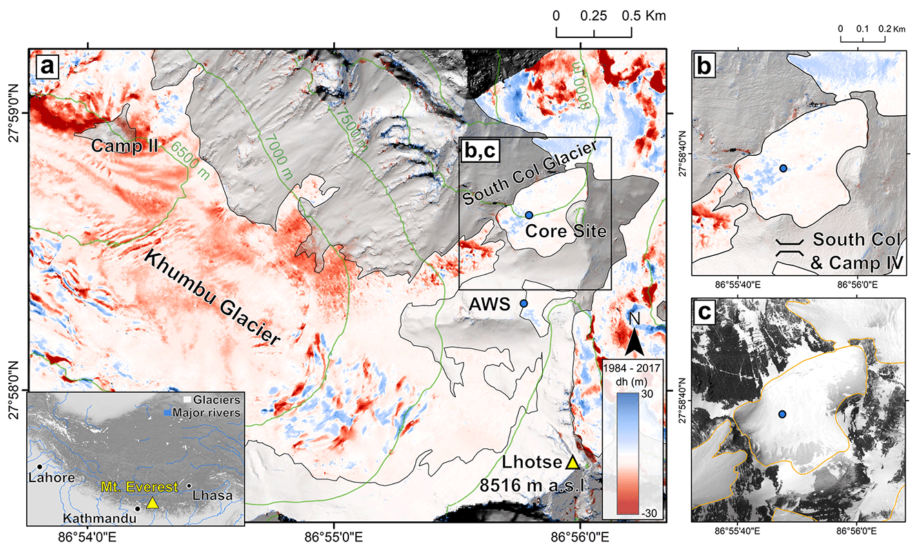
Figure 1Surface elevation change over the Western Cwm (a) between 1984 and 2017 and over the South Col Glacier (b). The locations of the ice core and AWS from Potocki et al. (2022) are shown with blue dots. Background is a shaded relief from the Pléiades DEM. The conditions at the surface of the South Col Glacier on 23 March 2017 are captured by a Pléiades orthoimage in panel (c). Pléiades, © CNES 2017, Distribution Airbus DS. Elevations are reported relative to the geoid. The inset in panel (a) shows the location of Mt. Everest.
The uncertainty associated with the mean elevation change over South Col Glacier (σdH,SCG) was estimated following Hugonnet et al. (2022). This robust approach applies error propagation for correlated variables considering, in the structure of error, the spatial correlation of errors at multiple ranges modeled by a variogram and the heteroscedasticity (i.e., variability in error) modeled by a variable variance , which is a function of the terrain slope α and maximum absolute curvature c:
where is the average of the variance of elevation differences in the glacier area A, composed of N pixels. is inferred by the square of the half difference between the 0.025 and 0.975 quantiles (a robust proxy for the 2σ uncertainty range) in binned categories of elevation differences on stable terrain. is the variogram of the standard score zdH on stable terrain (i.e., elevation differences standardized by σdH(α,c)), estimated by a median empirical variogram and modeled by a sum of two spherical models. The variogram of the standard score takes values between 0 (fully correlated) and 1 (uncorrelated) depending on the spatial lag di,j (i.e., distance between pixel i and j). We found that 89 % of the variance is correlated until a first range of 87 m, while the remaining 11 % are correlated until a second range of 6.5 km, after which errors are fully decorrelated.
Several patterns of dH are evident over the Western Cwm and South Col Glacier surroundings, which relate to both ice flow and surface mass balance processes (Fig. A1). The thinning and recession of the steep hanging glaciers on the north face of the Western Cwm are evident north of Camp II at an elevation of 6500 m a.s.l. (Fig. A1d–f). Slight (∼ 10 m or less) thinning is evident over the Khumbu Glacier up to an elevation of 7000 m a.s.l. Above this height, substantial elevation change is limited to areas where ice flow has driven crevasse field evolution between the two DEM dates, primarily on the Lhotse and Kangshung faces to the southwest and east of South Col Glacier, respectively (Fig. A1a–c). Over the South Col Glacier specifically, we find a mean elevation change of 0.01 ± 0.05 m a−1 for the period 1984–2017. The distribution of dH on South Col Glacier is rather homogeneous and not different from the distribution of dH over ice-free areas or over glacierized areas located within the same elevation range (Fig. A2). The distribution of elevation change values off ice centered around zero (mean of 0.07 m, standard deviation of 3.72 m) gives us confidence in the successful processing of both DEMs in the study area. Within a 50 m diameter circle centered on the drilling location of Potocki et al. (2022), the elevation change is 1.7 ± 5.1 m for the period 1984–2017, corresponding to an elevation change rate of 0.05 ± 0.15 m a−1. Glacier-wide and local (at drill site) thickness changes are thus statistically not different from zero (Fig. 1). This observation can be extended back in the past, at least in a qualitative way, as the comparison of photographs from the Swiss expedition to Everest in 1956 with photographs from 2008 and 2022 shows that there are no large changes visible in the thickness of South Col Glacier (Machguth and Mattea, 2022).
We investigate the mass balance processes to further understand the contending conclusions between the findings of Potocki et al. (2022) and our observations of no elevation change in South Col Glacier over the last 3 decades. Little is known about the surface mass balance processes at such high altitude, and consequently, we utilize multiple methods and data to investigate them. We first analyze high-temporal-resolution satellite images to document the seasonal evolution of the glacier surface state. We then model the potential magnitude of wind erosion, as it could be a very important process (Litt et al., 2019). Finally, we run a surface energy balance model with different configurations to investigate the significance of surface melt.
3.1 Seasonal surface state changes from satellite images
Due to its small size, highly reflective surface and persistent cloud coverage during monsoon (June, July, August and September: JJAS), the South Col Glacier is challenging to observe with standard optical satellite imagery. The VENµS satellite acquired multispectral images every 2 to 30 d from November 2017 to October 2020 that are suitable to qualitatively document the surface state changes in South Col Glacier (e.g., Bessin et al., 2022). VENµS images consist of 12 narrow spectral bands from blue visible (0.424 µm) to near-infrared (0.910 µm) with a 5 m ground resolution acquired at 11:00 local time (Dick et al., 2022).
We use 267 VENµS surface reflectance (SRE) multispectral images that we crop to the South Col Glacier surroundings. A total of 14 images with poor co-registration were horizontally shifted by manually selecting four GCPs. All other images are well co-registered and orthorectified in the original SRE product. We produce natural color composites using the band combination 7–4–3, corresponding to red, green and blue bands, respectively. The equalize_adapthist function from the Python scikit-image package was used to obtain a rendering that highlights the blue-ice areas (Fig. 2). We rely on visual inspection of the images only and did not attempt to automatically classify the snow-covered areas.
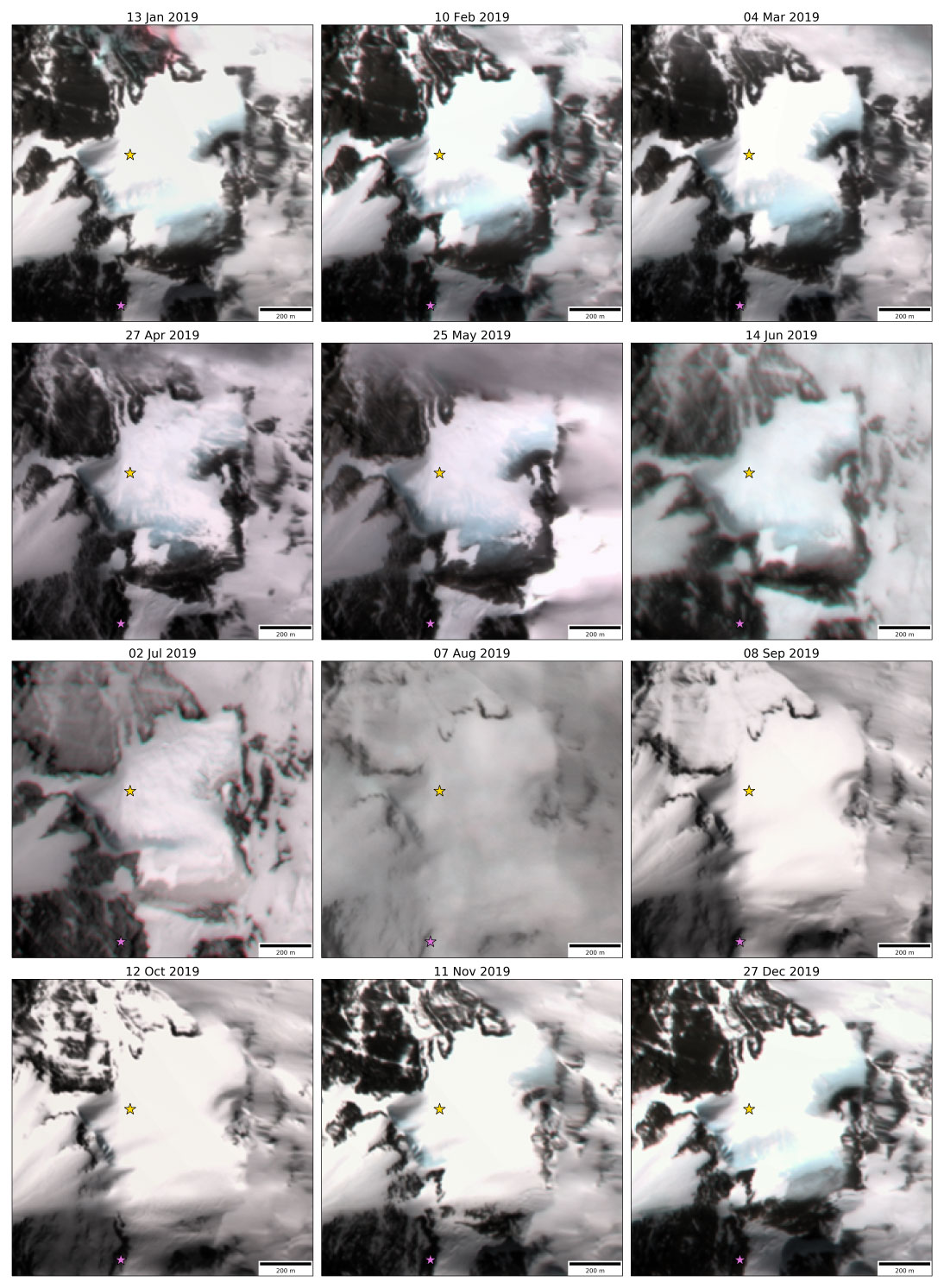
Figure 2Natural color composites (bands 7–4–3) of VENµS images (CC BY-NC 4.0) showing the seasonal variability in the surface snow cover of South Col Glacier. The yellow star shows the location of the drilling site and the purple one the location of the South Col AWS. Note the striking expansion of blue-ice areas outside the monsoon months, i.e., January–April 2019 and October–December 2019.
The South Col Glacier exhibits strong seasonal contrasts in terms of snow cover. Here we show only one image per month for the year 2019 (Fig. 2), but the whole image series is available (Brun, 2022). From January to June, the glacier surface is partially covered by snow, while ice is exposed in multiple places. The exposed ice area increases, at least until May and even sometimes June. After mid-June, the number of usable images is limited due to monsoon cloud cover, and the only image available in July shows that the glacier is covered by a thin layer of snow, as the ice is visible underneath. The glacier is then covered by an apparently thicker layer of snow in August, September and October. The ice is not visible, except at the lower cliff of South Col Glacier, above the Western Cwm (upper part of Khumbu Glacier, on the west side of South Col Glacier) in October. The ice re-appears in November, and its exposed area increases through the course of December (Fig. 2).
The series of VENµS images shows an excellent qualitative agreement with the albedo series measured at the South Col AWS in 2019 (Matthews et al., 2020). The South Col AWS (purple star in Fig. 2) was installed on a rock outcrop, which became covered by snow in early July 2019. Then the albedo of the surface below the AWS remained high until mid-October 2019, when the rock outcrop was re-exposed (Matthews et al., 2020).
With VENµS, we observe only 3 years (2018, 2019 and 2020), but our findings are similar for the 3 years. The qualitative interpretation of the VENµS image series hints at a dominant role of wind erosion in the surface mass balance. They show that late monsoon accumulation is removed during subsequent periods, as large blue-ice areas, starting at the east part of the glacier, become exposed within a few days in October–November when the available energy is limited for melt and when the wind speed is high.
3.2 The potential of wind erosion
In order to test the importance of wind erosion, we implement a simple model inspired from Amory et al. (2021). Hereafter we define accumulation as the snow that is deposited on the glacier surface (i.e., a fraction of precipitation) minus the erosion (i.e., the snow that is mechanically removed by wind from the glacier surface after the deposition). Accumulation can thus be negative when erosion exceeds deposition. The parameterization of wind erosion is based on a set of semi-empirical formulations, originally implemented in the polar-oriented regional climate model MAR (Gallée et al., 2001; Amory et al., 2021). MAR has been used to study the cryosphere under various climates, and the erosion and deposition processes have been largely validated in Antarctica where these processes are critical (e.g., Agosta et al., 2019). Here we develop a simplified analytical approach expressed in a one-dimensional vertical framework, in which the erosion model is only forced by the meteorological variables with no further interactions between the surface and the atmosphere. We assume that snow re-mobilized from the surface by wind is entirely exported off the glacier boundaries, which is justified by the local topography, with steep slopes around the glacier especially toward the east (predominant westerly winds). Due to its one-dimensional, offline nature, our analytical erosion model does not account for horizontal advection of airborne snow from upstream areas, and interactions of airborne snow particles with the atmosphere are neglected. Following Amory et al. (2021), fresh snow is assumed to be deposited with a density ρ of 300 kg m−3, the erosion rate is parameterized as a function of surface snow density and wind speed, and erosion is not allowed to occur when ρ≥450 kg m−3 or when the air temperature exceeds the freezing point. In this approach the snowpack is described with a three-layer model, representing a range of ρ values from fresh snow (top layer; ρ=300 kg m−3), erodible aging snow (intermediate layer; 300 kg m kg m−3) and non-erodible firn (bottom layer; ρ≥450 kg m−3). This ensures that the upper limit for the erosion rate is set to the mass content of the first two erodible layers and allows dense snow to be permanently added to the snowpack. Snow densification of the top layer is parameterized following a linear densification rate as implemented in MAR and is considered to occur under the action of erosion only. Note that our model does not resolve the surface energy balance and other mass balance processes (sublimation and melt), and it inherently ignores the related snow metamorphism. The snowpack is initialized as a single non-erodible firn layer. The model is described in more detail in Appendix A. The meteorological inputs (precipitation, wind speed, air temperature and surface pressure) required to drive the parametrization of wind erosion are directly taken from Potocki et al. (2022) and cover the period 1950–2019, as they originate from ERA5 downscaled data (Hersbach et al., 2020). However, instead of using artificially reduced precipitation (averaging 66.9 mm a−1) to implicitly account for wind erosion that is missing in Potocki et al. (2022), we prescribe uncorrected precipitation rates (averaging 191 mm a−1), as we intend to explicitly model wind erosion.
The dominant meteorological conditions at South Col Glacier were previously described (Matthews et al., 2020; Potocki et al., 2022). We focus on precipitation and wind, which both have a strong seasonal cycle (Fig. 3a). Most of the precipitation falls during the monsoon. In winter (December, January and February: DJF), the winds are extremely strong, with mean daily values approaching 20 m s−1 when the westerlies hit the topography (Maussion et al., 2014). During the monsoon, the winds progressively decrease, from a daily mean of around 10 m s−1 in early June to 2.5 m s−1 at the heart of the monsoon season (July and August). After mid-September, the wind speed increases very sharply, marking the end of the monsoon (Khadka et al., 2021). As a consequence, the precipitation falling before June is not deposited, and the accumulation efficiency (ratio of daily accumulation over precipitation, defined only when precipitation is non-zero) is close to zero (Fig. 3b). During the course of the monsoon, a large proportion of deposited precipitation is not eroded, and the accumulation efficiency gradually increases. The cumulative accumulation reaches a maximum in mid-September and ultimately decreases in October when winds strengthen again, meaning that erosion becomes larger than precipitation, thus leading to a negative accumulation efficiency (Fig. 3b). At that time of the year, in our model, the snow reaches a density of 450 kg m−3, which does not allow any additional erosion.
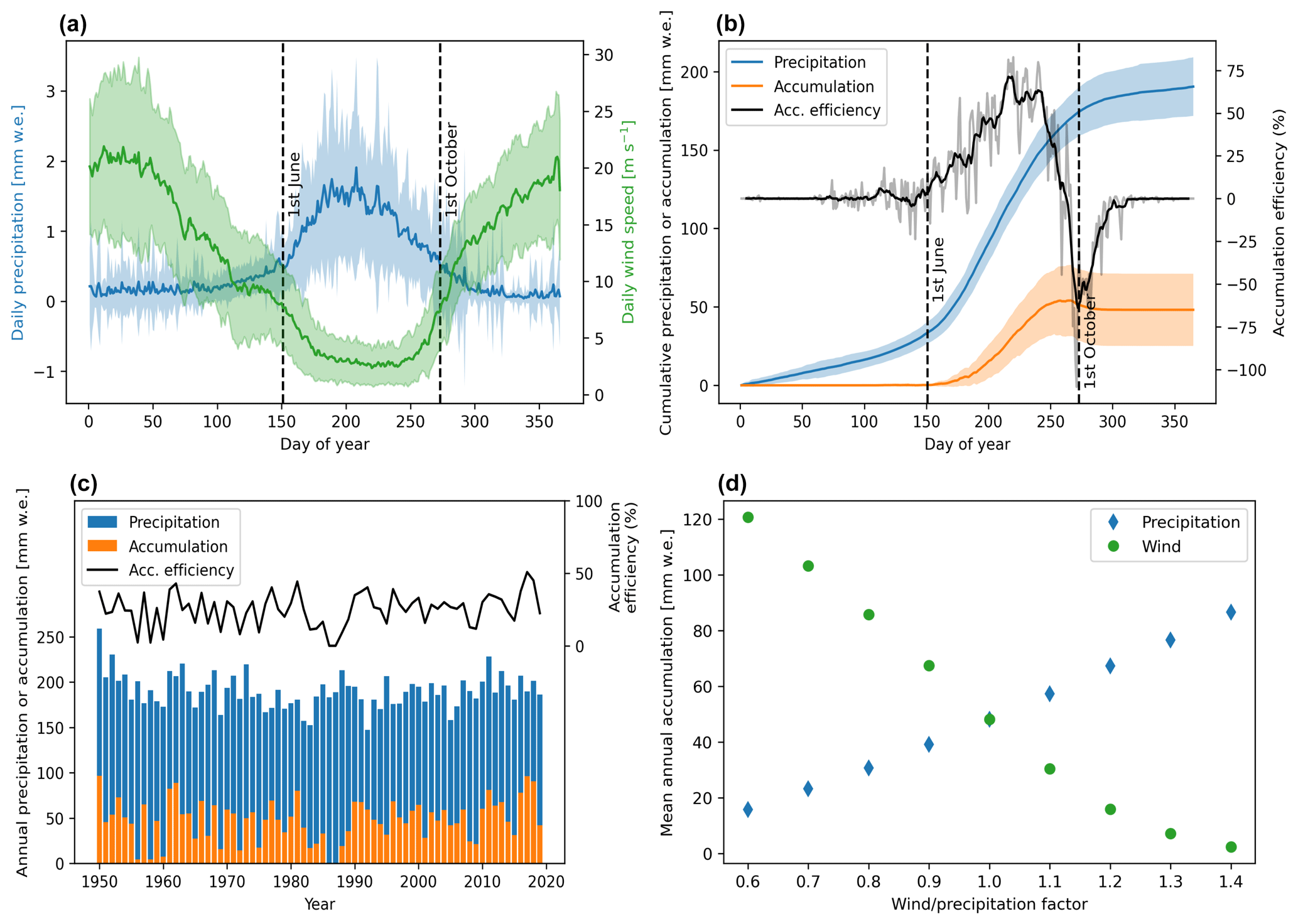
Figure 3Seasonal cycle of wind and precipitation from downscaled ERA5 data (a) and cumulative precipitation and accumulation from the wind erosion model (b) for the period 1950–2020. The black curve in panel (b) shows the 9 d moving average of the daily ratio of accumulation over precipitation. Panel (c) shows the annual values of precipitation, accumulation and accumulation efficiency. The model sensitivity to the wind and precipitation factors is shown in panel (d), where the averages are calculated for the period 1950–2020.
Over the period 1950–2019, the annual uncorrected precipitation ranges from 147 to 259 mm w.e., and only 0 % to 51 % (mean value 25 %) of the precipitation is deposited, ranging from 0 to 97 mm w.e. (mean value 48 mm w.e.), the rest being eroded by wind. The interannual variability in the accumulation efficiency is high, and the model results are very sensitive to the wind speed (Fig. 3c and d). With a wind speed increase of 30 % to 40 %, the annual accumulation is almost reduced to zero (Fig. 3d). Conversely, if the wind speed is 40 % lower, the mean annual accumulation is about 120 mm w.e., which is 63 % of the mean annual precipitation. The results are also very sensitive to the total amount of precipitation, with an increase of 40 % in precipitation corresponding to an increase in the accumulation of 80 % (Fig. 3d).
The wind erosion model is simple and has large limitations. It takes into account only wind erosion and time-dependent densification of snow, which regulates erosion. Despite these limitations, the results are in good qualitative agreement with the VENµS images. For instance, the pre-monsoon and early monsoon (MAM) snow on South Col Glacier disappears systematically in both the model and images. Then, the images show that the glacier is covered by snow during the core of the monsoon (August), which is when the model finds the highest accumulation efficiency (Fig. 3b). This pattern is conserved when testing the model sensitivity to the wind and precipitation input (Fig. A7). However, the images show erosion, or sublimation, during winter (Fig. A3). This is not reproduced in the model because snow density reaches the erosion limit of 450 kg m−3 imposed in the model.
From the analyses of the satellite images and the modeling of wind erosion, we conclude that large parts of the fallen snow are likely eroded or re-mobilized after deposition, adding a degree of complexity in the precipitation estimates. Potocki et al. (2022) used a stationary scaling factor to compute effective precipitation, whereas our analysis suggests that this should instead exhibit seasonality. The higher effective precipitation in the monsoon (from reduced wind speeds) that we find here would make it easier to re-establish a snowpack over the glacier – something that Potocki et al. (2022) inferred was unlikely to occur in their “ice” experiment. Hence, the South Col Glacier may not have thinned as Potocki et al. (2022) concluded because the high ice melt rates required do not have a chance to occur as the glacier surface remains snow covered throughout the monsoon.
Despite the availability of VENµS images, we cannot determine precisely the temporal share of ice exposed or snow-covered conditions for South Col Glacier. We therefore investigate the ablation processes by modeling the glacier mass balance over icy surfaces to consider a worst-case scenario that maximizes ablation (relative to a snow-covered scenario).
3.3 The challenge of modeling surface mass balance
Modeling the changes in ice or snow masses in response to atmospheric forcing is a complex task which involves resolving heat transport and conservation with concurrent phase changes (e.g., Anderson, 1976). There are many existing models in the literature which tackle the problem of coupling incoming energy fluxes with subsurface processes. Recent studies show the importance of this coupling to accurately model melt in the firn zone (e.g., Covi et al., 2022; Mattea et al., 2021; MacDonell et al., 2013). To model the surface mass balance of the South Col Glacier, Potocki et al. (2022) relied on the COSIPY model (Sauter et al., 2020). They notably found that, in the case of an all-year snow-free glacier surface, the COSIPY model predicts a substantial 1508 mm w.e. a−1 of melt on average for the simulation period 1950–2019. The goal of this section is to assess the robustness of this large modeled annual melt. For this purpose, we performed similar mass balance simulations of an ice surface with different model configurations. The purpose of the numerical simulations that we perform in this section is not to produce realistic estimates of the surface mass balance prevailing at South Col Glacier but to show that various acceptable choices in the numerical treatment of the surface energy balance in COSIPY produce very different results in terms of melt.
We compare two different model configurations forced with the same meteorological inputs, taken from Potocki et al. (2022), to simulate the ice ablation for the year 2019 (arbitrarily chosen). Note that simulations are performed over only 1 year, as the aim is to investigate the fundamental potential of large melt rather than mimic the entire long-term melt evolution. For that, we first use the standard version of COSIPY run with an hourly time step, as in Potocki et al. (2022). This simulation is named hereafter COSIPY_P22, and it is not exactly identical to the outputs of Potocki et al. (2022) due to minor updates in COSIPY code. We then used a slightly modified version of COSIPY with (i) a 1 min time step and (ii) a modified computation of the heat conduction flux between the surface and the ice below that is incorrectly referred to as the ground heat flux in COSIPY (Sauter et al., 2020) and in Potocki et al. (2022). Indeed, in the default COSIPY settings used in Potocki et al. (2022), the heat conduction flux is computed by considering the temperature gradient on the first 10 cm of the ice column. However, physically this heat conduction flux is driven by the temperature gradient right under the surface (Sauter et al., 2020). We thus modify the COSIPY source code to compute the temperature gradient as close as possible to the surface. Specifically, we use the temperature values at the surface and at the node below (usually at 1 cm depth) in order to compute the temperature gradient in the vicinity of the surface. This simulation is named hereafter COSIPY_grad. In order to maintain an icy surface in COSIPY_grad, we set the precipitation to zero, thus maintaining albedo at its minimum value and likely enhancing melt. The COSIPY_grad simulation is initialized with the thermal state predicted by a COSIPY simulation similar to COSIPY_P22 that ran from 1 January 2010 to 1 January 2019. At the start of the simulation the snow thickness is zero, and the domain consists only of impermeable ice.
COSIPY_P22 predicts a significant amount of melt (918 mm w.e. for the year 2019), while COSIPY_grad only predicts 15 mm w.e. a−1 (Fig. 4). This large difference cannot be accounted for by differences in the radiative or turbulent fluxes, as they are similar for both simulations (Fig. A4). In particular, the daily sublimation rate is very close for both simulations with a cumulative sublimation of 453 and 482 mm w.e. simulated by COSIPY_P22 and COSIPY_grad, respectively, for the year 2019. Furthermore, in both simulations, the surface reaches the melting point during daytime in the monsoon period (Fig. 4), but only COSIPY_P22 predicts a large amount of melt. The simulated surface temperatures are very close when comparing the hourly averages, with COSIPY_grad being slightly warmer than COSIPY_P22 (RMSE = 2.2 K; mean difference = −0.1 K). However, the daily maxima of COSIPY_P22 are on average 2.1 K higher than COSIPY_grad (Fig. 4).
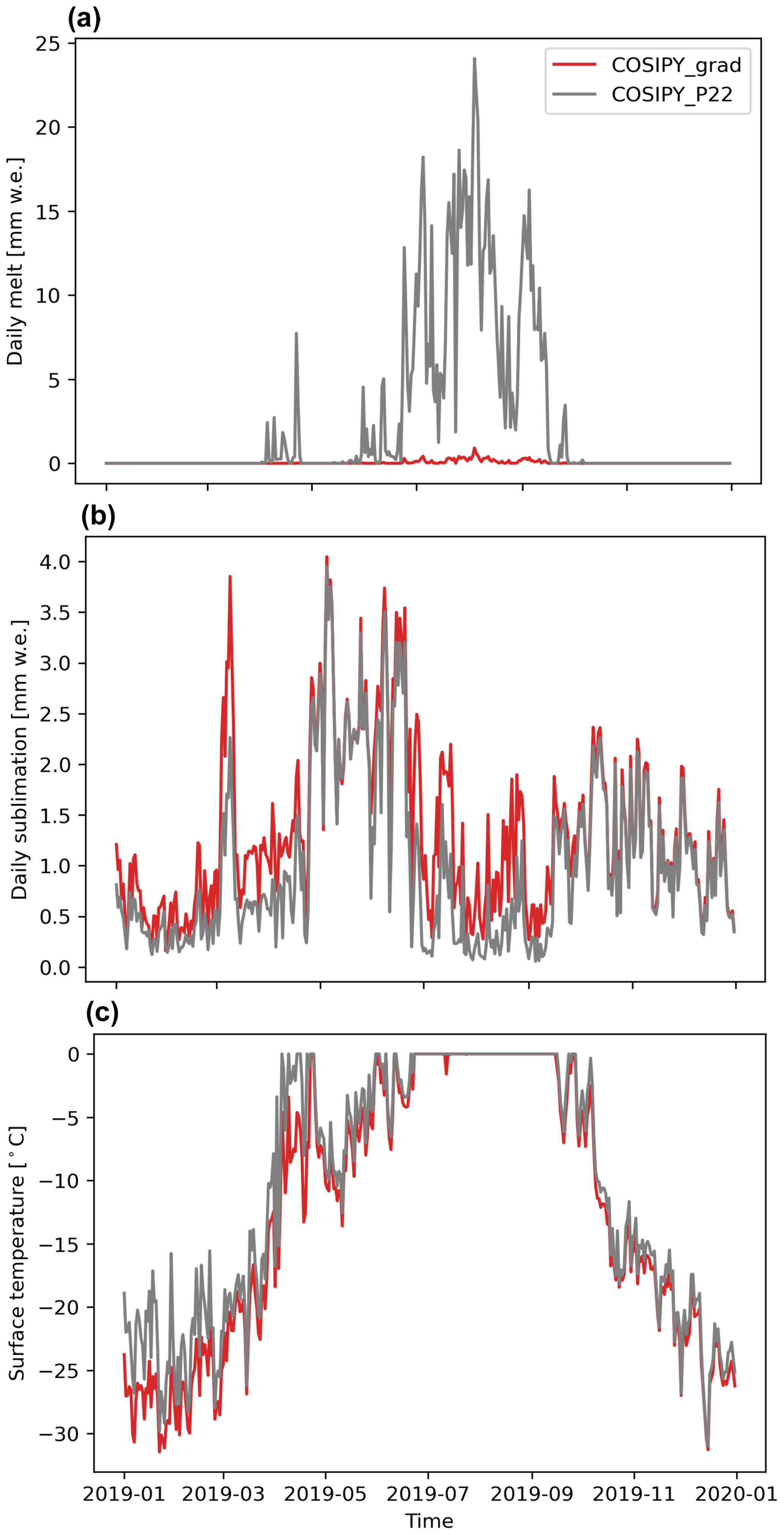
Figure 4Daily melt rate (a), sublimation rate (b) and maximum daily surface temperature (c) simulated by P22 (grey) and COSIPY_grad (red) models for the year 2019. Daily rates are computed from the hourly sum. The daily surface temperature corresponds to the maximum simulated during the day. Note that the initial thermal state is identical for all simulations and is estimated by a COSIPY simulation similar to P22 that ran from 1 January 2010 to 1 January 2019.
As both simulations predict surface temperature reaching melting temperature and similar surface fluxes, the discrepancies between their predicted melt can likely be explained by differences in the representation of energy transport. In both COSIPY versions the surface temperature is computed by searching for the temperature that equilibrates the energy fluxes at the surface. If the equilibrium temperature is above the melting point, the surface temperature is capped at the melting temperature and the excess energy is used for melting the surface. The computation of this equilibrium temperature requires the amount of energy transported by conduction from the surface into the ice column to be computed, the so-called ground heat flux in Sauter et al. (2020) and Potocki et al. (2022) actually representing the subsurface heat conduction flux. As explained above, in the standard COSIPY version this subsurface heat conduction flux is estimated using the first 10 cm of the ice column and is therefore potentially not representative of the strong temperature gradient that can be present in the direct vicinity (i.e., the first centimeters) of the surface. This can lead to an underestimation of the subsurface heat conduction flux affecting the amount of energy accumulated at the surface and, in this case, favoring melt. This phenomenon is further exacerbated by the use of an hourly time step, the decoupling of the energy absorption and the internal heat diffusion processes in COSIPY: energy is accumulated during a full hour before it can be removed by internal diffusion, leading to temperature and melt overshoots. The reduction in the time step to a minute in COSIPY_P22 reduces the predicted melt by about 30 % (Fig. A5). We note that the simulation at 1 h time step and a temperature gradient calculated very close to the surface lead to an unrealistically high mean annual subsurface heat flux (i.e., 600 W m−2 compared to the annual mean incoming shortwave radiation below 300 W m−2 for the same period). The calculation of the temperature gradient close to the surface, in combination with a smaller time step, allows the model to efficiently evacuate energy from the surface, hindering melting. As seen in Fig. A6, the COSIPY_grad simulation predicts much higher subsurface heat conduction fluxes during the monsoon period, strongly limiting the surface melt.
This numerical experiment demonstrates that the structure and physical implementation of a model can strongly affect the way the energy is spatially allocated and transported, leading to large variations in predicted melt despite solving, in principle, the same physical processes. Notably, the COSIPY_grad simulation highlights that physically consistent modeling configurations can lead to little melt when considering the energy budget of an ice surface under the conditions of South Col Glacier. However, we raise some awareness about the parametrization choices made for the simulation, such as, for instance, the albedo, that increase the model uncertainty. Indeed, the ice of South Col Glacier appears blue and might have a larger albedo than 0.4, as is observed for blue-ice-type albedos that can reach 0.5 to 0.6 (e.g., Smedley et al., 2020). A higher ice albedo would dramatically reduce the melt totals, as suggested by the sensitivity tests of Potocki et al. (2022) and Machguth and Mattea (2022). In view of the large modeling uncertainty and without measurements, it is therefore not possible to definitively draw conclusions on the amount of surface melting when ice is exposed on South Col Glacier (i.e., when snow-free conditions are observed in June and potentially July) solely from a modeling point of view. Additionally, even though there would be some surface melt on this glacier, it is likely that a large amount of this meltwater would refreeze at the surface in the case of the presence of snow or firn or would form superimposed ice. While COSIPY accounts for refreezing in snow, it considers water originating from an ice surface as runoff, limiting its applicability in such a cold context. We thus highlight here that COSIPY does not seem to be suitable to model mass balance in the specific conditions of South Col Glacier without extensive validation.
In the original interpretation of the South Col Glacier ice core, Potocki et al. (2022) dated the top 10–69 cm of the core and found an age of 1966 ± 179 years. Based on a layer-counting estimate of annual accumulation of 27 mm w.e. a−1, they concluded that ∼ 55 m of ice were missing and had been removed. Relying on surface mass balance modeling with COSIPY, they estimated contemporary local mass balance rates approaching −2 m a−1 and thus dated the initiation of thinning to the 1990s. The interpretation of Potocki et al. (2022) relies on two assumptions: (i) a continuous and stable accumulation of ∼ 27 mm w.e. a−1 for a 2000-year period and (ii) the absence of ice flow and ice emergence that would transport old ice from the accumulation zone to the surface of the ablation zone.
Regarding (i), given the small value for accumulation and the magnitude of and variability in wind erosion, it seems difficult to accept that accumulation is stable and continuous. Moreover, the accumulation is estimated based on 10 m of ice, which would consequently correspond to an approximate duration of only 330 years. The assumption that similar surface mass balance conditions persisted for up to the last 2000 years is therefore based on a large extrapolation. If the accumulation was not continuous – i.e., if there are some missing years in the core records – then the ice that is 1966 ± 179 years old exposed near to the surface would not imply 55 m of missing ice. More precise dating of the deeper sections of the South Col Glacier ice core could help resolve the question of continuity of accumulation. Note that our present study focuses on the period 1984–2017 (or 1956–2022; Machguth and Mattea, 2022) when no thinning is observed, but we cannot exclude any thickening and/or thinning episodes anterior to this period, potentially explaining why Potocki et al. (2022) observed ice as old as 1966 ± 179 years at the surface of their ice core.
Regarding (ii), Potocki et al. (2022) neglected ice flow and thus did not distinguish surface mass balance and elevation and/or thickness change. However, South Col Glacier is flowing at an unknown velocity as evidenced by the presence of a bergschrund, large crevasses and primary stratification visible on the Pléiades orthoimage (Fig. 1c). Given that the ice core has a mean density of 890 kg m−3 and that no firn is mentioned in Potocki et al. (2022), we wonder whether the core could have been drilled in an area of the glacier where ablation conditions frequently prevail. As a consequence, the divergence of ice flux would be negative and ice would emerge, leading to old ice being exposed at the surface. One possible interpretation is that avalanches occurring at the foot of Everest's southeast face feed an area of the glacier with dense snow that is more difficult to erode, leading to a local excess of mass and thus actual accumulation. For the rest of the glacier area, erosion and sublimation, which are both controlled by wind, maintain a near-zero balance between accumulation and ablation.
Furthermore, finding ice that is as old as 1966 ± 179 years at the surface suggests that South Col Glacier is flowing very slowly. Given that the distance between the bergschrund and the drilling site is approximately 150 m (Fig. A1), ice as old as 1966 ± 179 years cannot be encountered in the core if the average horizontal velocity exceeds m a−1. We do not know where this ice formed along the flow line, so the velocity is likely lower than this maximum estimate of 0.08 m a−1. The South Col Glacier is thus likely a glacier with small ice fluxes. This would be in good agreement with our modeling of wind erosion and surface mass balance suggesting arid conditions. A large fraction of precipitation (>60 %) is eroded, limiting accumulation. Then sublimation is likely the dominant ablation process that removes 90 to 450 mm w.e. of snow or ice per year (this study and Potocki et al., 2022), leading to a very limited mass turnover (i.e., low absolute value of surface mass balance), in agreement with small ice fluxes (e.g., Cuffey and Paterson, 2010).
In our study, we demonstrate on the basis of remote sensing information that no significant elevation change occurred at South Col Glacier between 1984 and 2017. This is in contrast with the strong rates of melt (or thinning) postulated by Potocki et al. (2022) of almost 2 m a−1 at the location of the ice core during the recent past. Our results show that high melt rates are unlikely to happen on South Col Glacier for two main reasons: (i) the glacier is covered by snow during most of the monsoon season, limiting the net incoming shortwave radiation, and (ii) the glacier did not thin over the last 3 decades, and the ice core analysis suggests low velocities and thus low mass turnover. Moreover, when the glacier surface consists of exposed ice, which is the case where highest melt is expected due to low albedo, the magnitude of melt is highly dependent on modeling choices (i.e., model structure and parameters) for similar meteorological inputs, and the COSIPY model structure might not be well suited for this particular application.
The surface mass balance processes happening in the extreme meteorological context of South Col Glacier are complex, and our study does not reach any definitive conclusion about the relative importance of each of these processes. The lack of direct observations hampers our ability to decipher the dominant glaciological processes and thus to model the glacier recent and future evolution in a realistic way. Specifically, stake measurements would be needed to measure the surface mass balance and surface velocity in a direct way; ground penetrating radar measurements would help constrain the ice thickness; and a number of subsurface temperature, snow-depth, snow transport or turbulent flux measurements would help constrain the processes. Without more observational knowledge, it appears currently very difficult to draw a conclusion on the sensitivity of South Col Glacier to climate change or to predict its future evolution.
The contribution of the wind erosion of snow to the local glacier mass balance results from three-dimensional interactions of the atmospheric flow with the surface which thus, in principle, cannot be properly treated with a one-dimensional model. Although the erosion process, which describes the removal of snow from the surface by wind, may be expressed in a one-dimensional vertical framework, the net export of snow by horizontal transport, however, needs resolving in the horizontal dimensions by definition. Due to the relatively small dimensions of the glacier (0.2 km2) and its complex topographical surroundings, capturing the erosion process over this full range of spatial scales requires an eddy-resolving, three-dimensional model with a very fine, meter-scale horizontal resolution and appropriate lateral boundary fluxes. This approach would also require a very large amount of computational resources and is thus not suited for climatological timescales. As a much more computationally efficient alternative, we used a simplified approach to parameterize wind erosion of snow as a one-dimensional vertical model.
Our parameterization is inspired from the erosion scheme of the regional climate model MAR (Gallée et al., 2001; Amory et al., 2021) and assumes a complete export of eroded snow outside of the glacier boundaries by horizontal wind transport. This assumption is crude but has some theoretical support. Due to the geometry and the northeast–southwest orientation of the South Col Glacier (Fig. 1), westerlies are the dominant and strongest local winds (Fig. A8) as a result of local topographical channeling. They may thus mostly be responsible for snow erosion and export off the eastern side of the glacier. An illustration of this process is the striking expansion of blue-ice surfaces revealed by the analysis of VENµS images during the last quarter of the year 2019 (Fig. 2), when strong wind speeds of high erosive potential occur after the monsoon season. Another way to support this assumption is to confirm that a snow model equipped with a parameterization of wind erosion can reproduce this feature.
Wind erosion is usually considered to initiate when the friction velocity, u* (m s−1), exceeds a threshold value, u*t (m s−1), mostly determined by snow microstructural characteristics at the surface including snow density, grain size, and bond number and strength (Schmidt, 1980). In our model, the friction velocity u* is derived from the 2 m local wind speed forcing U, directly taken from Potocki et al. (2022) and assuming a logarithmic wind profile:
where k is the von Kármán constant (0.4) and z0 the roughness length for momentum set to 10−4 m. Following Amory et al. (2021), in the absence of observational characterization of local surface snow characteristics, the threshold friction velocity u*t is expressed as a function of snow surface density only:
with u*t0 the expression for the standard friction velocity (0.211 m s−1), ρice the density of ice (920 kg m−3), ρ0 the density of fresh snow (set to 300 kg m−3) and ρs the density of surface snow (kg m−3).
When , the air temperature is below the freezing point, and the surface snow density is below 450 kg m−3 (see below), the particle ratio in the saltation layer qsalt (kg kg−1; mass of saltating snow particles per unit mass of atmosphere) is computed as a function of the excess of shear stress responsible for the removal of snow particles from the surface:
where g=9.81 is the gravitational acceleration (m s−2), is the height of the saltation layer (m), and is the saltation efficiency expressed as a dimensionless coefficient inversely proportional to the friction velocity. A surface turbulent flux of snow, referred to as potential erosion Ep (m s−1 kg kg−1), is then approximated assuming that it follows a bulk formula:
where CD is a drag coefficient (10−3) similar to that used for sensible and latent heat fluxes, U is the near-surface wind at the standard level (10 m), and qs is the snow particle ratio (kg kg−1) at the same level. Assuming that any re-mobilized snow is quickly removed by horizontal transport, then , and, re-expressing U assuming a logarithmic wind profile, Ep is given by
Equation (A3) contains semi-empirical formulations assumed to implicitly account for all the physical processes that contribute the airborne snow mass, including the gravitational settling of snow particles. Equation (A5) expresses turbulent vertical exchange between the saltation layer and the overlying atmosphere but not settling. However, the saltation layer contains significant quantities of snow under strong winds (Nemoto and Nishimura, 2004; Huang et al., 2016), in which case turbulence is a dominant contributor over settling that is consequently ignored. We then deduce an expression for the maximum amount of erodible snow ER (kg m−2) during one time step dt (1 h):
where is the density of air (kg m−3), P the surface pressure (Pa), R=287 the specific gas constant (J kg−1 K−1) and T the air temperature (K). The effective erosion EReff (kg m−2) is then taken as the minimum between the maximal erosion ER and the available snow mass for erosion (mass content in the top and intermediate layer) in the snow model. Note that u*t is recomputed for each snow layer. If a layer is completely eroded during a time step, the layer below is also eroded during the same time step. The maximal erosion ER of this layer is then computed taking into account the time spent to erode the upper layer.
In natural environments, wind erosion contributes to the densification of the snow surface due to the combined actions of wind and saltation which break original crystal shapes and favor the formation of smaller, rounded snow grains (Sato et al., 2008), leading to enhanced sintering, more efficient mechanical packing and increased density (Vionnet et al., 2013). Erosion-induced densification and the exposure of denser snow or ice layers through erosion both naturally contribute to reduce the likelihood of additional erosion. In our model, erosion-induced densification is applied to the top snow layer that has experienced erosion following a linear densification rate from the fresh snow value ρ0 (assumed to be representative of snow that has been barely altered by post-depositional processes) to the prohibitive density value for snow erosion ρmax:
where ρmax=450 kg m−3 and τER is the characteristic timescale for erosion-induced densification set to 24 h. As our model time step (1 h) is small compared to τER, the negative feedback of snow erosion within one time step can be neglected and is only active from one time step to another.
After the densification step, if the snow density exceeds the density criteria of the layer, it is transferred to the next denser layer. When snow is moved from the top layer to the intermediate layer, the density of the intermediate layer is recomputed by weighted average of the former thicknesses of each layers.
Our model is a simplified approach aiming at quantifying the effect of wind erosion on the mass balance of the South Col Glacier. Other ablation processes (melt, sublimation) resulting from the surface energy balance, snow metamorphism processes and snowpack internal changes in snow characteristics which can lead to additional densification are neglected. However, we expect few implications since erosion of a snow layer of density above ρmax of 450 kg m−3 is prohibited. Even if some internal model parameters (ρ0, ρmax, τER) have been scaled for Antarctic conditions (Amory et al., 2021), we simply re-used without additional tuning the original configuration of MAR, considering the similarities in the climatological context between coastal Antarctica and the South Col Glacier (extreme wind speeds and relatively low air temperatures).
The erosion parameterization proposed above is admittedly very approximate. It ignores notably the sublimation of airborne snow (Gallée et al., 2001). However, as we assume a complete export of drifting snow, whether the suspended snow is finally exported in the solid or vapor phase makes no difference. Although other formulations of wind erosion could be devised, a more constrained parameterization could not necessarily be developed without additional measurements or through a coupling with a multidimensional model and/or a multilayer snow model. Our main point here is that, in order to explain the gradual removal of snow and resulting appearance of blue-ice areas as revealed from analysis of VENµS images and to understand the reasons behind its temporal variability, it is necessary to account for wind erosion.
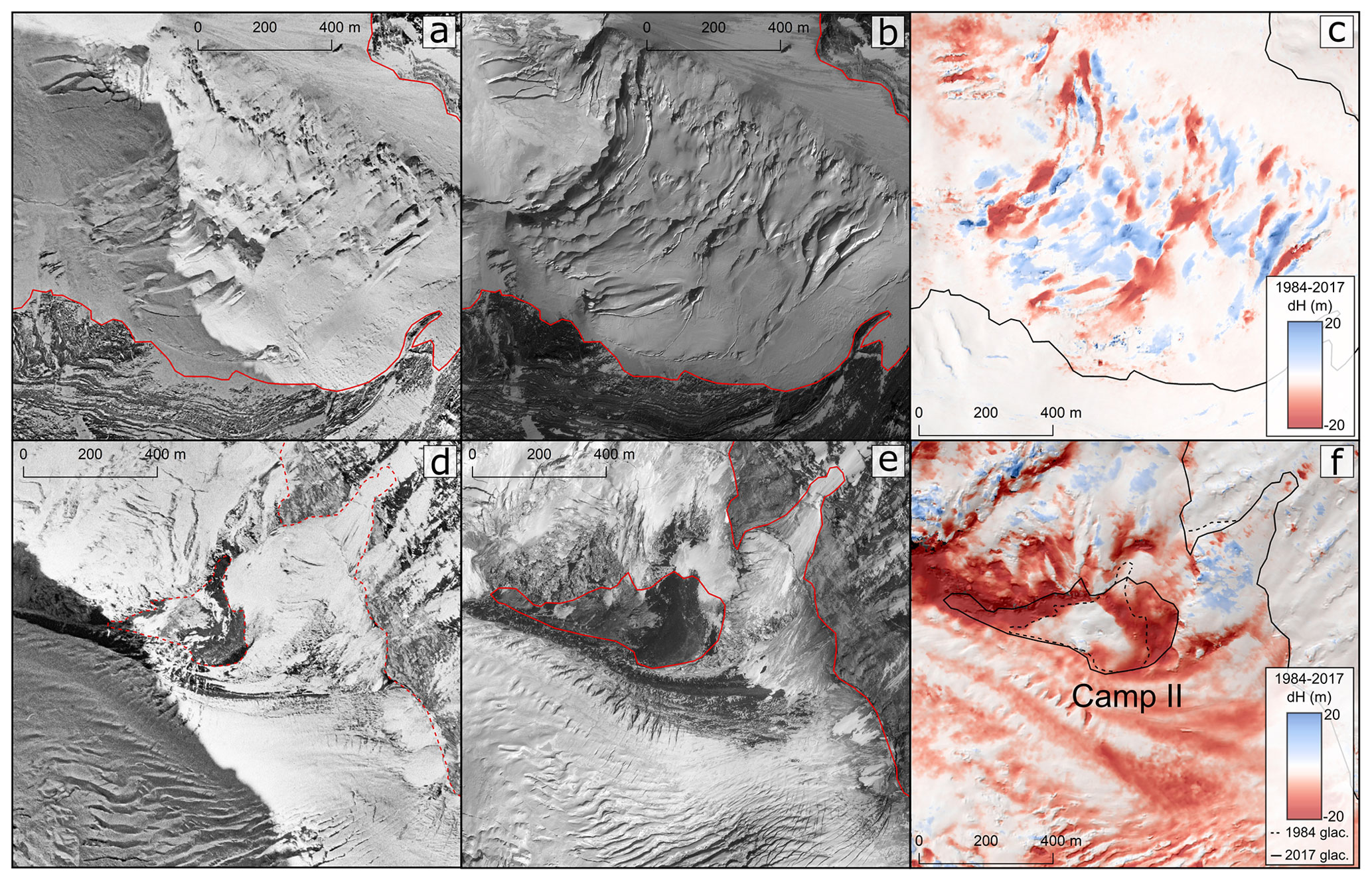
Figure A1Examples of glacier surface conditions captured by aerial photographs (1984) and Pléiades imagery (2017) in the Western Cwm and associated changes in surface elevation. (a–c) Crevassing of the Lhotse face in 1984 (a) and 2017 (b) and corresponding elevation change estimates (c) over the same period. The alternating positive and negative elevation difference pattern reflects the movement, opening and/or closure of crevasses. (d–f) The expansion of the area of exposed bedrock around Camp II between 1984 (d) and 2017 (e) and associated elevation changes (f). Shadows prominent in panels (a) and (d) illustrate the wintertime acquisition date of the aerial photographs compared to the spring (23 March) acquisition of the Pléiades imagery (panels b and e). Pléiades, copyright CNES 2017, Distribution Airbus DS.
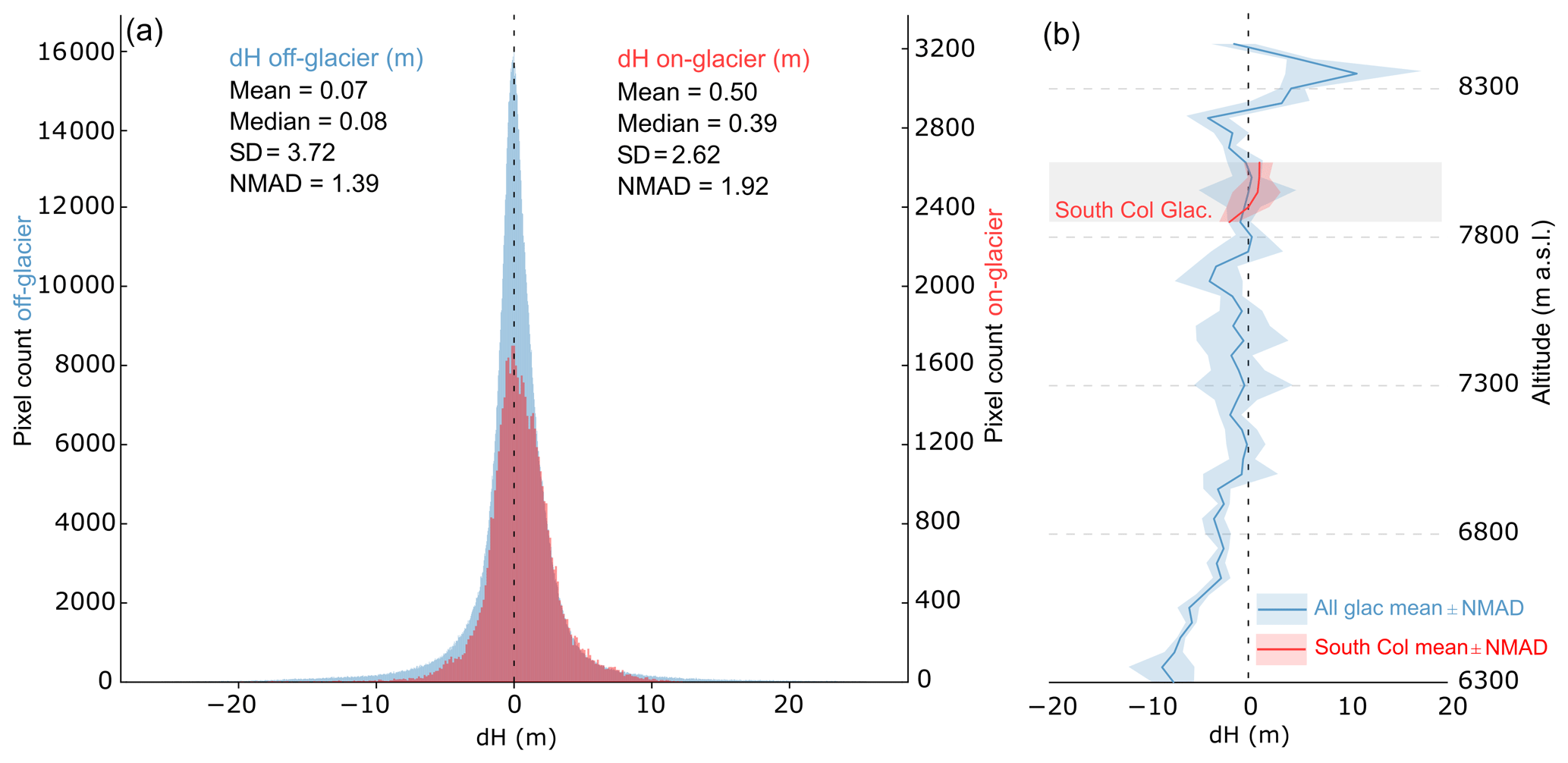
Figure A2Distribution of the elevation change values off-glacier and on South Col Glacier (a). Elevation changes for 1984–2017 as a function of elevation for every 50 m elevation bin for the whole glacierized area and for South Col Glacier (b).
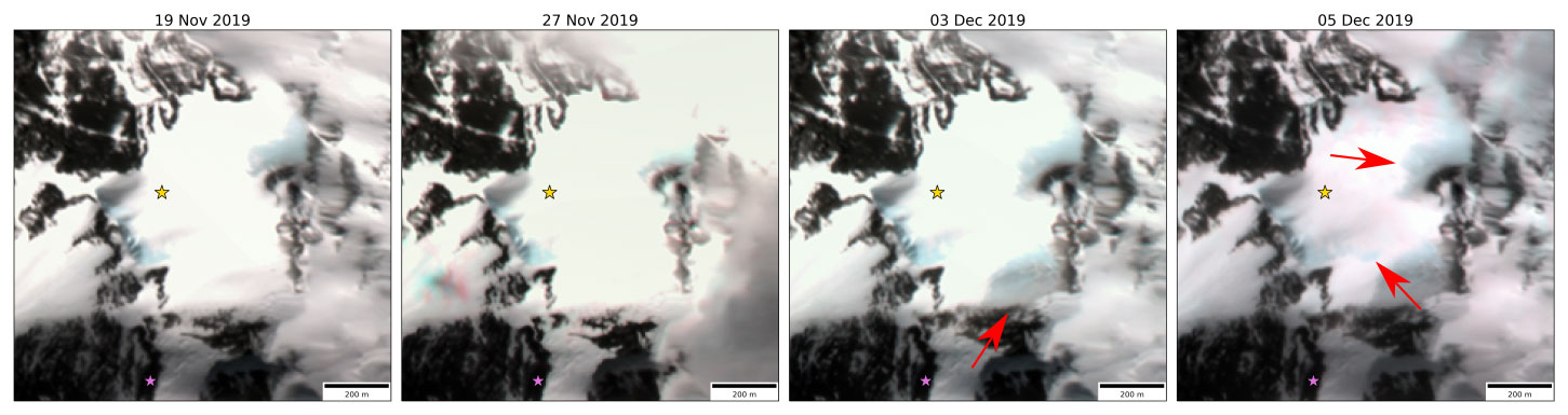
Figure A3Natural color composites (bands 7–4–3) of VENµS images (CC BY-NC 4.0) showing episodes of snow cover loss in November and December 2019. The yellow star shows the location of the drilling site and the purple one the location of the South Col AWS. The red arrows point to the areas of large changes.
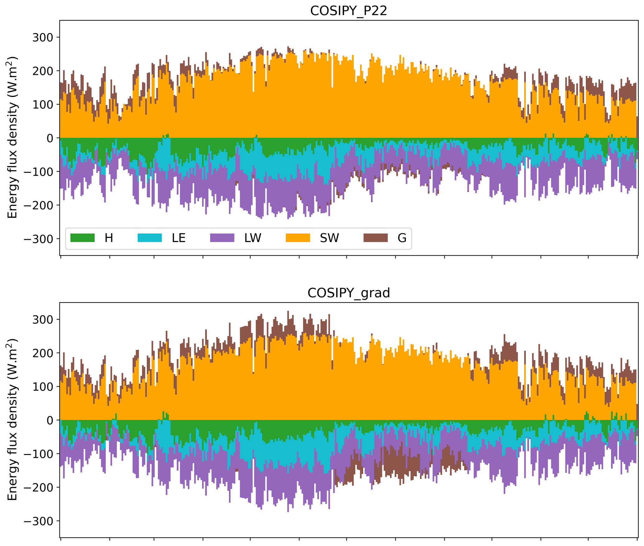
Figure A4Day-of-year mean energy fluxes for the ice simulations with COSIPY_P22 and COSIPY_grad for the year 2019.
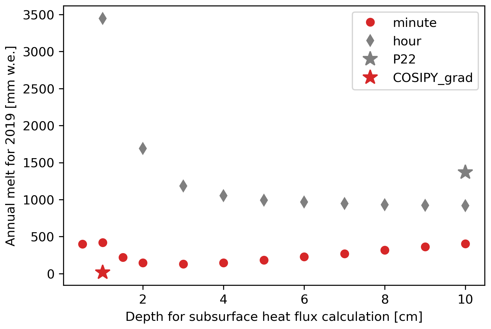
Figure A5Sensitivity of the annual melt for the year 2019 to the choice of the temperature interpolation depth (zlt2) in COSIPY. Note that the parameter zlt1 is set as zlt2/2. The red symbols correspond to simulations run at a 1 min time step, and the grey ones correspond to simulations run at a 1 h time step. P22 is the original simulation from Potocki et al. (2022).
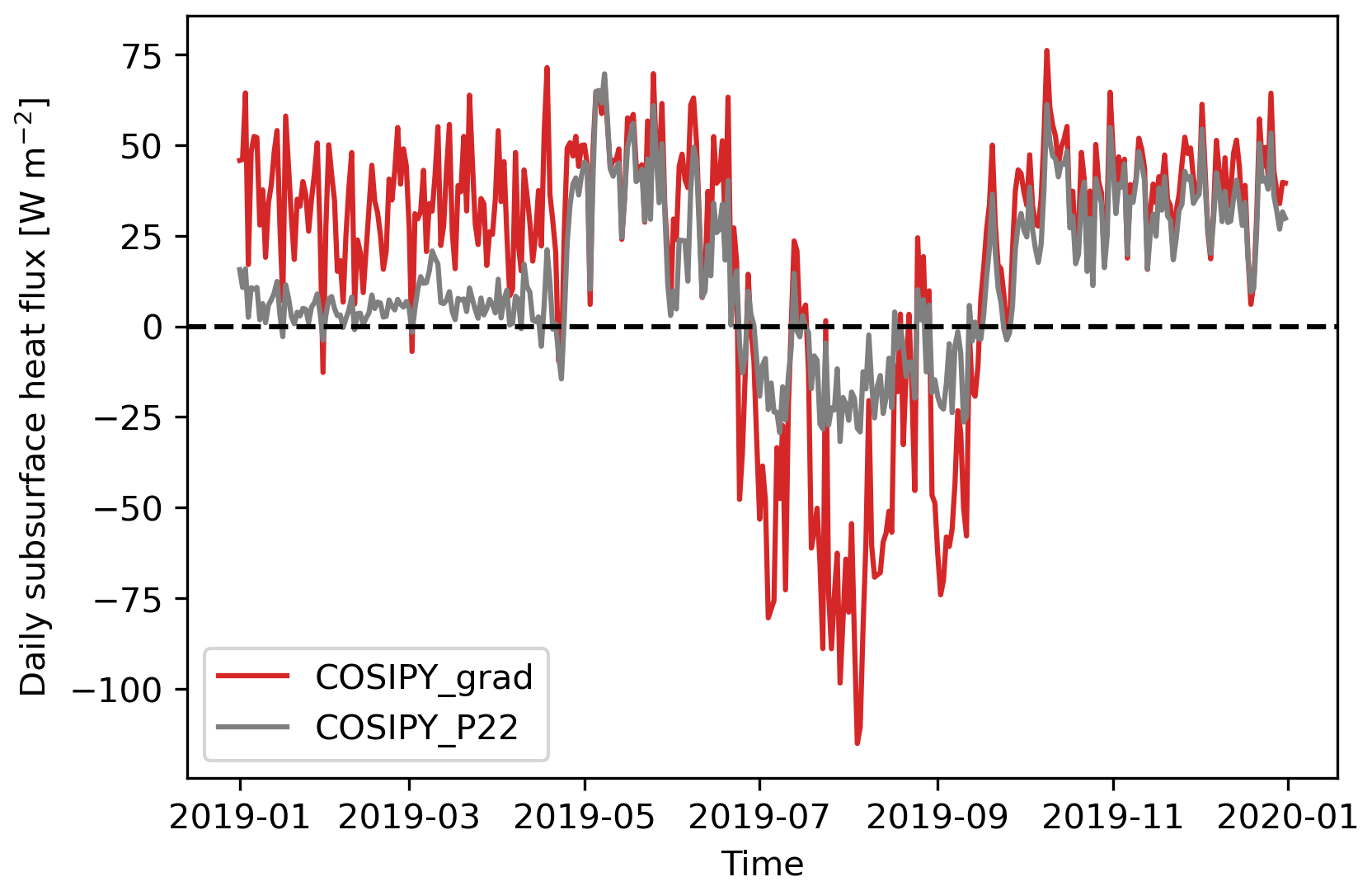
Figure A6Daily averages of ground heat flux for the COSIPY_P22 and the COSIPY_grad simulations.
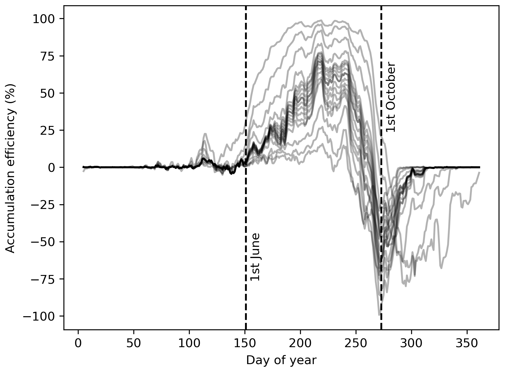
Figure A7Accumulation efficiency averaged over the period 1950–2020. Each line represents one simulation with a varying wind or precipitation factor. All the lines are smoothed with a 9 d running mean.
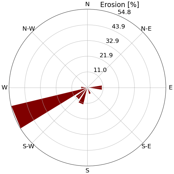
Figure A8Erosion as a function of wind direction for the period when wind data are available from the AWS, showing the dominant role of west-southwest winds.
The dH map is on a public repository, together with the aerial photograph DEM (https://doi.org/10.5281/zenodo.7529761, King, 2023). The Pléiades DEM is available at https://doi.org/10.5281/zenodo.6979691 (Berthier, 2022). License restrictions apply to the Pléiades orthoimages, which are available upon request to Etienne Berthier, pending the signature of a license agreement with CNES.
The uncertainty analysis code is available at https://github.com/rhugonnet/uncertainty_analysis_SCG/blob/main/uncert_SCG_from_Hugonnet2022.ipynb (last access: 9 August 2023), and, based on the Python package, xDEM is available at https://github.com/GlacioHack/xdem (last access: 9 August 2023; DOI: https://doi.org/10.5281/zenodo.8220229, Hugonnet, 2023).
VENµS data are available at https://doi.org/10.5281/zenodo.6685515 (Brun, 2022).
The wind erosion code is available at https://github.com/antonplanchot/wind-snow-scg (Planchot and Amory, 2023).
Mass balance simulations presented in this study are available at https://doi.org/10.5281/zenodo.7006744 (Réveillet et al., 2022).
FB, MR and CA designed the study. OK, EB, FB, AD and RH generated the DEMs and analyzed DEM differences; MR, KF, JB, FB and MD analyzed the results of the surface mass balance models; and CA and AP developed the wind erosion model and analyzed the results. SL analyzed the Sentinel-1 backscatter series (not shown in the article). FB led the writing, and all the authors contributed to it. TB, CM and PW discussed the interpretation of the results.
At least one of the (co-)authors is a member of the editorial board of The Cryosphere. The peer-review process was guided by an independent editor, and the authors also have no other competing interests to declare.
Publisher’s note: Copernicus Publications remains neutral with regard to jurisdictional claims in published maps and institutional affiliations.
CNRM/CEN is part of Labex OSUG@2020. We thank Evan Miles, Fabien Maussion and Vincent Favier for insightful discussions and comments on the initial version of this work. We thank the editors (Francesca Pellicciotti and Thomas Mölg), the five reviewers (including Ann Rowan, Horst Machguth and Martin Lüthi), Enrico Mattea, Marcus Gastaldello, Nicolas Steiner and the authors of Potocki et al. (2022) for insightful and constructive comments and discussions which improved the quality of this article.
This research has been supported by the European Research Council (ERC) under the European Union's Horizon 2020 research and innovation program (IVORI; grant no. 949516), the French Space Agency (CNES), and the ANR for the iFROG project (grant no. ANR-21-CE01-0012).
This paper was edited by Thomas Mölg and reviewed by Horst Machguth, Ann Rowan, Martin Lüthi, and two anonymous referees.
Agosta, C., Amory, C., Kittel, C., Orsi, A., Favier, V., Gallée, H., van den Broeke, M. R., Lenaerts, J. T. M., van Wessem, J. M., van de Berg, W. J., and Fettweis, X.: Estimation of the Antarctic surface mass balance using the regional climate model MAR (1979–2015) and identification of dominant processes, The Cryosphere, 13, 281–296, https://doi.org/10.5194/tc-13-281-2019, 2019. a
Amory, C., Kittel, C., Le Toumelin, L., Agosta, C., Delhasse, A., Favier, V., and Fettweis, X.: Performance of MAR (v3.11) in simulating the drifting-snow climate and surface mass balance of Adélie Land, East Antarctica, Geosci. Model Dev., 14, 3487–3510, https://doi.org/10.5194/gmd-14-3487-2021, 2021. a, b, c, d, e, f
Anderson, E. A.: A point energy and mass balance model of a snow cover, https://repository.library.noaa.gov/view/noaa/6392 (last access: 9 August 2023), 1976. a
Berthier, E.: Pléiades DEM of 23 March 2017 – Khumbu region, Nepal, Zenodo [data set], https://doi.org/10.5281/zenodo.6979691, 2022. a
Berthier, E., Vincent, C., Magnússon, E., Gunnlaugsson, Á. Þ., Pitte, P., Le Meur, E., Masiokas, M., Ruiz, L., Pálsson, F., Belart, J. M. C., and Wagnon, P.: Glacier topography and elevation changes derived from Pléiades sub-meter stereo images, The Cryosphere, 8, 2275–2291, https://doi.org/10.5194/tc-8-2275-2014, 2014. a
Bessin, Z., Dedieu, J.-P., Arnaud, Y., Wagnon, P., Brun, F., Esteves, M., Perry, B., and Matthews, T.: Processing of VENµS Images of High Mountains: A Case Study for Cryospheric and Hydro-Climatic Applications in the Everest Region (Nepal), Remote Sensing, 14, 1098, https://doi.org/10.3390/rs14051098, 2022. a
Beyer, R. A., Alexandrov, O., and McMichael, S.: The Ames Stereo Pipeline: NASA's Open Source Software for Deriving and Processing Terrain Data, Earth and Space Science, 5, 537–548, https://doi.org/10.1029/2018EA000409, 2018. a
Brun, F.: Natural color composites of VENµS images over South Col Glacier, Zenodo [data set], https://doi.org/10.5281/zenodo.6685515, 2022. a, b
Covi, F., Hock, R., and Reijmer, C.: Challenges in modeling the energy balance and melt in the percolation zone of the Greenland ice sheet, J. Glaciol., 69, 164–178, https://doi.org/10.1017/jog.2022.54, 2022. a
Cuffey, K. M. and Paterson, W. S. B.: The physics of glaciers, Academic Press, ISBN 9780123694614, 2010. a
Dick, A., Raynaud, J.-L., Rolland, A., Pelou, S., Coustance, S., Dedieu, G., Hagolle, O., Burochin, J.-P., Binet, R., and Moreau, A.: VENµS: Mission Characteristics, Final Evaluation of the First Phase and Data Production, Remote Sensing, 14, 3281, https://doi.org/10.3390/rs14143281, 2022. a
Gallée, H., Guyomarc'h, G., and Brun, E.: Impact Of Snow Drift On The Antarctic Ice Sheet Surface Mass Balance: Possible Sensitivity To Snow-Surface Properties, Bound.-Lay. Meteorol., 99, 1–19, https://doi.org/10.1023/A:1018776422809, 2001. a, b, c
Hersbach, H., Bell, B., Berrisford, P., Hirahara, S., Horányi, A., Muñoz‐Sabater, J., Nicolas, J., Peubey, C., Radu, R., and Schepers, D.: The ERA5 global reanalysis, Q. J. Roy. Meteor. Soc., 146, 1999–2049, https://doi.org/10.1002/qj.3803, 2020. a
Hirschmuller, H.: Stereo Processing by Semiglobal Matching and Mutual Information, IEEE T. Pattern Anal., 30, 328–341, https://doi.org/10.1109/TPAMI.2007.1166, 2008. a
Huang, N., Dai, X., and Zhang, J.: The impacts of moisture transport on drifting snow sublimation in the saltation layer, Atmos. Chem. Phys., 16, 7523–7529, https://doi.org/10.5194/acp-16-7523-2016, 2016. a
Hugonnet, R.: Uncertainty calculation for South Col Glacier geodetic mass balance, Zenodo [data set], https://doi.org/10.5281/zenodo.8220229, 2023. a
Hugonnet, R., McNabb, R., Berthier, E., Menounos, B., Nuth, C., Girod, L., Farinotti, D., Huss, M., Dussaillant, I., Brun, F., and Kääb, A.: Accelerated global glacier mass loss in the early twenty-first century, Nature, 592, 726–731, https://doi.org/10.1038/s41586-021-03436-z, 2021. a, b
Hugonnet, R., Brun, F., Berthier, E., Dehecq, A., Mannerfelt, E. S., Eckert, N., and Farinotti, D.: Uncertainty Analysis of Digital Elevation Models by Spatial Inference From Stable Terrain, IEEE J. Sel. Top. Appl., 15, 6456–6472, 2022. a
IPCC: Climate Change 2021: The Physical Science Basis. Contribution of Working Group I to the Sixth Assessment Report of the Intergovernmental Panel on Climate Change, Cambridge University Press, Cambridge, United Kingdom and New York, NY, USA, in press, https://doi.org/10.1017/9781009157896, 2021. a
Khadka, A., Matthews, T., Perry, L. B., Koch, I., Wagnon, P., Shrestha, D., Sherpa, T. C., Aryal, D., Tait, A., Sherpa, T. G., Tuladhar, S., Baidya, S. K., Elvin, S., Elmore, A. C., Gajurel, A., and Mayewski, P. A.: Weather on Mount Everest during the 2019 summer monsoon, Weather, 76, 205–207, https://doi.org/10.1002/wea.3931, 2021. a
King, O.: 1984 Digital Elevation Model and 1984–2017 surface elevation change grids over the Western Cwm of Mt Everest, Zenodo [data set], https://doi.org/10.5281/zenodo.7529761, 2023. a
King, O., Bhattacharya, A., Ghuffar, S., Tait, A., Guilford, S., Elmore, A. C., and Bolch, T.: Six Decades of Glacier Mass Changes around Mt. Everest Are Revealed by Historical and Contemporary Images, One Earth, 3, 608–620, https://doi.org/10.1016/j.oneear.2020.10.019, 2020. a, b
Litt, M., Shea, J., Wagnon, P., Steiner, J., Koch, I., Stigter, E., and Immerzeel, W.: Glacier ablation and temperature indexed melt models in the Nepalese Himalaya, Scientific Reports, 9, 5264, https://doi.org/10.1038/s41598-019-41657-5, 2019. a
MacDonell, S., Kinnard, C., Mölg, T., Nicholson, L., and Abermann, J.: Meteorological drivers of ablation processes on a cold glacier in the semi-arid Andes of Chile, The Cryosphere, 7, 1513–1526, https://doi.org/10.5194/tc-7-1513-2013, 2013. a
Machguth, H. and Mattea, E.: Review of tc-2022-166, https://doi.org/10.5194/tc-2022-166-rc4, 2022. a, b, c
Mattea, E., Machguth, H., Kronenberg, M., van Pelt, W., Bassi, M., and Hoelzle, M.: Firn changes at Colle Gnifetti revealed with a high-resolution process-based physical model approach, The Cryosphere, 15, 3181–3205, https://doi.org/10.5194/tc-15-3181-2021, 2021. a
Matthews, T., Perry, L. B., Koch, I., Aryal, D., Khadka, A., Shrestha, D., Abernathy, K., Elmore, A. C., Seimon, A., Tait, A., Elvin, S., Tuladhar, S., Baidya, S. K., Potocki, M., Birkel, S. D., Kang, S., Sherpa, T. C., Gajurel, A., and Mayewski, P. A.: Going to Extremes: Installing the World’s Highest Weather Stations on Mount Everest, B. Am. Meteorol. Soc., 101, E1870–E1890, https://doi.org/10.1175/BAMS-D-19-0198.1, 2020. a, b, c, d
Maussion, F., Scherer, D., Mölg, T., Collier, E., Curio, J., and Finkelnburg, R.: Precipitation Seasonality and Variability over the Tibetan Plateau as Resolved by the High Asia Reanalysis, J. Climate, 27, 1910–1927, https://doi.org/10.1175/JCLI-D-13-00282.1, 2014. a
Nemoto, M. and Nishimura, K.: Numerical simulation of snow saltation and suspension in a turbulent boundary layer, J. Geophys. Res., 109, D18206, https://doi.org/10.1029/2004JD004657, 2004. a
Nuth, C. and Kääb, A.: Co-registration and bias corrections of satellite elevation data sets for quantifying glacier thickness change, The Cryosphere, 5, 271–290, https://doi.org/10.5194/tc-5-271-2011, 2011. a
Planchot, A. and Amory, C.: Three layer wind erosion model for South Col Glacier, GitHub [code], https://github.com/antonplanchot/wind-snow-scg, last access: 9 August 2023. a
Potocki, M., Mayewski, P. A., Matthews, T., Perry, L. B., Schwikowski, M., Tait, A. M., Korotkikh, E., Clifford, H., Kang, S., Sherpa, T. C., Singh, P. K., Koch, I., and Birkel, S.: Mt. Everest’s highest glacier is a sentinel for accelerating ice loss, npj Climate and Atmospheric Science, 5, 7, https://doi.org/10.1038/s41612-022-00230-0, 2022. a, b, c, d, e, f, g, h, i, j, k, l, m, n, o, p, q, r, s, t, u, v, w, x, y, z, aa, ab, ac, ad, ae, af, ag
Réveillet, M., Brun, F., Fourteau, K., Brondex, J., and Dumont, M.: Simulation outputs associated to the study: “Brief communication: Everest South Col Glacier did not thin during the last three decades” by Brun et al., Zenodo [data set], https://doi.org/10.5281/zenodo.7006744, 2022. a
Sakai, A.: Brief communication: Updated GAMDAM glacier inventory over high-mountain Asia, The Cryosphere, 13, 2043–2049, https://doi.org/10.5194/tc-13-2043-2019, 2019. a
Sato, T., Kosugi, K., S., M., and M., N.: Wind speed dependences of fracture and accumulation of snowflakes on snow surface, Cold Reg. Sci. Technol., 51, 229–239, https://doi.org/10.1016/j.coldregions.2007.05.004, 2008. a
Sauter, T., Arndt, A., and Schneider, C.: COSIPY v1.3 – an open-source coupled snowpack and ice surface energy and mass balance model, Geosci. Model Dev., 13, 5645–5662, https://doi.org/10.5194/gmd-13-5645-2020, 2020. a, b, c, d
Schmidt, R. A.: Threshold wind-speeds and elastic impact in snow transport, J. Glaciol., 26, 453–467, https://doi.org/10.3189/S0022143000010972, 1980. a
Smedley, A. R. D., Evatt, G. W., Mallinson, A., and Harvey, E.: Solar radiative transfer in Antarctic blue ice: spectral considerations, subsurface enhancement, inclusions, and meteorites, The Cryosphere, 14, 789–809, https://doi.org/10.5194/tc-14-789-2020, 2020. a
Vincent, C., Gilbert, A., Jourdain, B., Piard, L., Ginot, P., Mikhalenko, V., Possenti, P., Le Meur, E., Laarman, O., and Six, D.: Strong changes in englacial temperatures despite insignificant changes in ice thickness at Dôme du Goûter glacier (Mont Blanc area), The Cryosphere, 14, 925–934, https://doi.org/10.5194/tc-14-925-2020, 2020. a
Vionnet, V., Guyomarc’h, G., Naaim Bouvet, F., Martin, E., Durand, Y., Bellot, H., Bel, C., and Puglièse, P.: Occurrence of blowing snow events at an alpine site over a 10-year period: Observations and modelling, Adv. Water Resour., 55, 53–63, https://doi.org/10.1016/j.advwatres.2012.05.004, 2013. a
Washburn, B.: Mapping Mount Everest, Bulletin of the American Academy of Arts and Sciences, 42, 29–44, https://doi.org/10.2307/3824352, 1989. a
Zemp, M., Huss, M., Thibert, E., Eckert, N., McNabb, R., Huber, J., Barandun, M., Machguth, H., Nussbaumer, S. U., Gärtner-Roer, I., Thomson, L., Paul, F., Maussion, F., Kutuzov, S., and Cogley, J. G.: Global glacier mass changes and their contributions to sea-level rise from 1961 to 2016, Nature, 568, 382–386, https://doi.org/10.1038/s41586-019-1071-0, 2019. a
- Abstract
- Introduction
- South Col Glacier elevation change
- Surface mass balance processes
- Implications for the interpretation of the South Col Glacier ice core
- Conclusions
- Appendix A: Parameterizing wind erosion
- Code and data availability
- Author contributions
- Competing interests
- Disclaimer
- Acknowledgements
- Financial support
- Review statement
- References