the Creative Commons Attribution 4.0 License.
the Creative Commons Attribution 4.0 License.
 | 04 Jul 2023
Seasonal variability in Antarctic ice shelf velocities forced by sea surface height variations
Cyrille Mosbeux
Laurie Padman
Emilie Klein
Peter D. Bromirski
Helen A. Fricker
Antarctica's ice shelves resist the flow of grounded ice towards the ocean through “buttressing” arising from their contact with ice rises, rumples, and lateral margins. Ice shelf thinning and retreat reduce buttressing, leading to increased delivery of mass to the ocean that adds to global sea level. Ice shelf response to large annual cycles in atmospheric and oceanic processes provides opportunities to study the dynamics of both ice shelves and the buttressed grounded ice. Here, we explore whether seasonal variability of sea surface height (SSH) can explain observed seasonal variability of ice velocity. We investigate this hypothesis using several time series of ice velocity from the Ross Ice Shelf (RIS), satellite-based estimates of SSH seaward of the RIS front, ocean models of SSH under and near RIS, and a viscous ice sheet model. The observed annual changes in RIS velocity are of the order of 1–10 m a−1 (roughly 1 % of mean flow). The ice sheet model, forced by the observed and modelled range of SSH of about 10 cm, reproduces the observed velocity changes when sufficiently large basal drag changes near the grounding line are parameterised. The model response is dominated by grounding line migration but with a significant contribution from SSH-induced tilt of the ice shelf. We expect that climate-driven changes in the seasonal cycles of winds and upper-ocean summer warming will modify the seasonal response of ice shelves to SSH and that nonlinear responses of the ice sheet will affect the longer trend in ice sheet response and its potential sea-level rise contribution.
- Article
(9177 KB) - Full-text XML
-
Supplement
(7595 KB) - BibTeX
- EndNote


The Antarctic Ice Sheet discharges mass via outlet glaciers and ice streams flowing into the ocean across the grounding lines, forming ice shelves several hundreds of metres thick, surrounding about half of the Antarctic coastline (Allison et al., 2011; Fretwell et al., 2013). Ice shelves play critical roles in ice sheet dynamics by providing back stresses that impede the gravity-forced flow of grounded ice towards the grounding line (Thomas, 1979). Ice shelf extent, thickness, and mass can vary over time (e.g. Cook and Vaughan, 2010; Paolo et al., 2015; Adusumilli et al., 2020), leading to changes in ice velocity for both grounded and floating ice (e.g. Scambos et al., 2004; Fürst et al., 2016; Reese et al., 2018; Gudmundsson et al., 2019). Persistent ice shelf thinning or retreat over years or decades can lead to a significant increase in the rate of mass loss of grounded ice (e.g. Velicogna et al., 2014; Joughin et al., 2014; Gudmundsson et al., 2019; Smith et al., 2020) and an associated increase in the rate of Antarctica's contribution to global sea level.
Time series of ice velocity (uice) from Global Navigation Satellite System (GNSS) receivers mounted on grounded and floating ice are, typically, of fairly short duration, limited to ∼1–3 months over austral summer. These short records reveal a strong tidal-band signal (e.g. Makinson et al., 2012) but cannot resolve annual cycles. However, a few longer GNSS records (e.g. Klein et al., 2020) and satellite-based estimates of uice (Greene et al., 2018, 2020) show variability on intra-annual (monthly to seasonal) timescales. Given that the seasonal cycle dominates variability in atmospheric and oceanic forcing of ice shelves, understanding how this forcing cycle affects ice shelf flow may provide important insights into the processes affecting the ice shelves and ice sheets and how they might respond to the weaker but more persistent forcing at longer timescales, from interannual variability (e.g. Dutrieux et al., 2014; Paolo et al., 2018) to multi-decadal trends (Jenkins et al., 2018).
Two mechanisms have been proposed to explain seasonal variability in ice shelf flow, linked to seasonal variability in (i) basal melt rates and (ii) sea ice. Klein et al. (2020) investigated the hypothesis that a seasonal cycle of spatially varying basal melt rates on the Ross Ice Shelf (Tinto et al., 2019; Stewart et al., 2019) might result in seasonality of uice; however, their modelled variability of uice was much smaller than GNSS measurements indicated. Greene et al. (2018) proposed that changes in buttressing from sea ice could explain the satellite-derived seasonal cycle of Totten Glacier's ice shelf; however, their uncertainties in satellite-derived intra-annual uice estimates were large, and the mechanism of ice shelf buttressing by sea ice is poorly understood.
In this paper, we investigate an alternative hypothesis: seasonal variability of sea surface height (SSH) modifies ice velocity through a combination of sea surface tilt and changing basal stresses at the grounding zone. This hypothesis is motivated by an extension of the role of tides in ice shelves and grounded-ice motion (Gudmundsson, 2007, 2013; Brunt and MacAyeal, 2014; Rosier and Gudmundsson, 2020), evidence from open ocean satellite altimetry that SSH around Antarctica has a pronounced seasonal cycle (Armitage et al., 2018; Rye et al., 2014) and the recent development of ocean models from which estimates of seasonal variability of SSH under ice shelves can be extracted. We explore our hypothesis by running a viscous model of the ice sheet and ice shelf in the Ross Sea sector with forcing from the modelled seasonal cycle of SSH under the Ross Ice Shelf and comparing the model output with GNSS time series of ice shelf velocity. We selected the Ross Ice Shelf because variability in ice shelf mass balance at longer timescales is known to be small (Das et al., 2020; Adusumilli et al., 2020), and there are several GNSS records exceeding 1 year in length that reveal intra-annual variability (e.g. Siegfried et al., 2014a; Bromirski et al., 2017; Blewitt et al., 2018). We show that the ice sheet model reproduces the observed annual cycle of the GNSS records if a sufficiently large cycle of SSH-induced basal shear stress change near the grounding line is parameterised in our viscous model. SSH-induced tilt of the ice shelf provides a small but significant additional contribution to velocity changes.
We explore our hypothesis using a combination of in situ and satellite-derived observations, as well as ocean and ice sheet modelling. We take advantage of several existing GNSS records from the Ross Ice Shelf (RIS) collected during various field campaigns (Sect. 2.1), focusing on the ones that are sufficiently long to identify intra-annual velocity variations. We combine these records with estimates of intra-annual variations in SSH fields for the open ocean in front of the ice shelves from an existing satellite altimetry data set and from ocean models that include ice shelves (Sect. 2.2). We then compare the GNSS records to an ice flow model forced with the varying SSH from the ocean models (Sect. 2.3).
2.1 GNSS data
We use several long (5–19 months) time series of ice shelf motion from GNSS deployments on RIS (Fig. 1). These records were collected during different time intervals between 2014 and 2019 (Table 1). GNSS data from all stations were processed with a precise point positioning (PPP) approach (Zumberge et al., 1997; Geng et al., 2012, 2019).
DRRIS 2015–2016. An array of 13 GNSS stations was deployed on RIS from November 2015 to December 2016 as part of the Dynamic Response of the Ross Ice Shelf to Wave-induced Vibrations (DRRIS) project (Bromirski et al., 2017; Klein et al., 2020). Three stations were deployed along the ice front and nine along a flowline from the central ice front station to about 400 km upstream. One station (RS03) was located 100 km to the west of the along-flowline array and another (RS08) was on grounded ice on the western margin of Roosevelt Island. Only one station (DR10) recorded position data for a full year; however, the intra-annual signals in positions and velocities at the other DRRIS stations on floating ice were highly correlated with DR10 observations (Klein et al., 2020, their Fig. 6).
WISSARD 2014–2016. An array of GNSS stations was deployed as part of the Whillans Ice Stream Subglacial Access Research Drilling (WISSARD; Siegfried et al., 2014a; Tulaczyk et al., 2014) project. We used the record from station GZ19 located about 3 km offshore of the Whillans Ice Stream grounding line, which acquired data between November 2014 and November 2016 (Begeman et al., 2020).
Antarctica PI continuous network 2017–2019. Two GNSS stations (BATG and LORG) acquired data in the northwestern RIS. We obtained the time series for these sites from the GNSS database processed by the Nevada Geodetic Laboratory (NGL; Blewitt et al., 2018). Station BATG was located about 100 km east of Minna Bluff and acquired data from February 2017 to August 2018. Station LORG was located about 100 km east of Ross Island and about 90 km from BATG; the station recorded from November 2018 to November 2019 with a few interruptions, for a total of 289 d. The vertical components of tidal variability at these stations were reported by Ray et al. (2021).
Table 1Station latitudes and longitudes at the time of deployment, mean speed, project and/or database which collected the data, duration (number of days of available data), and periods of deployment for GNSS stations. The primary stations used in this study are indicated in bold.
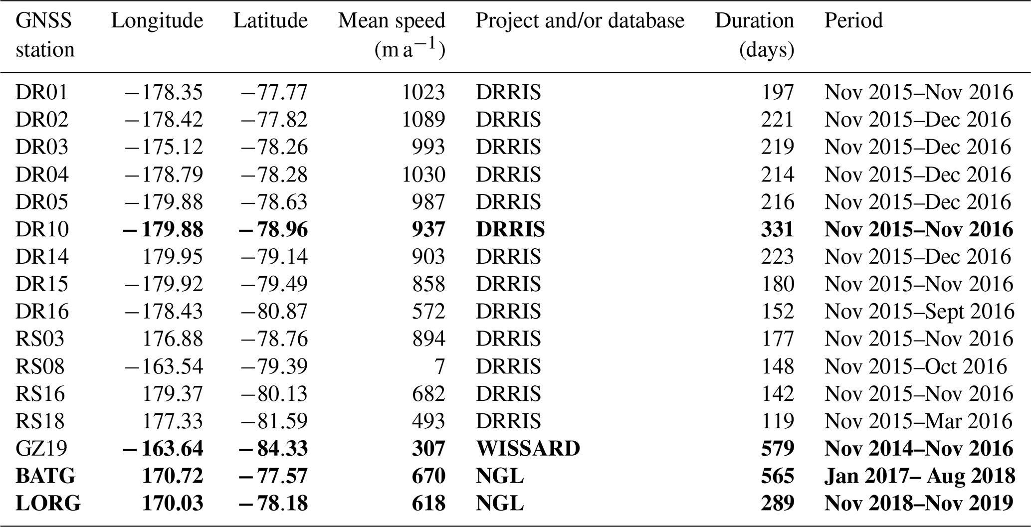
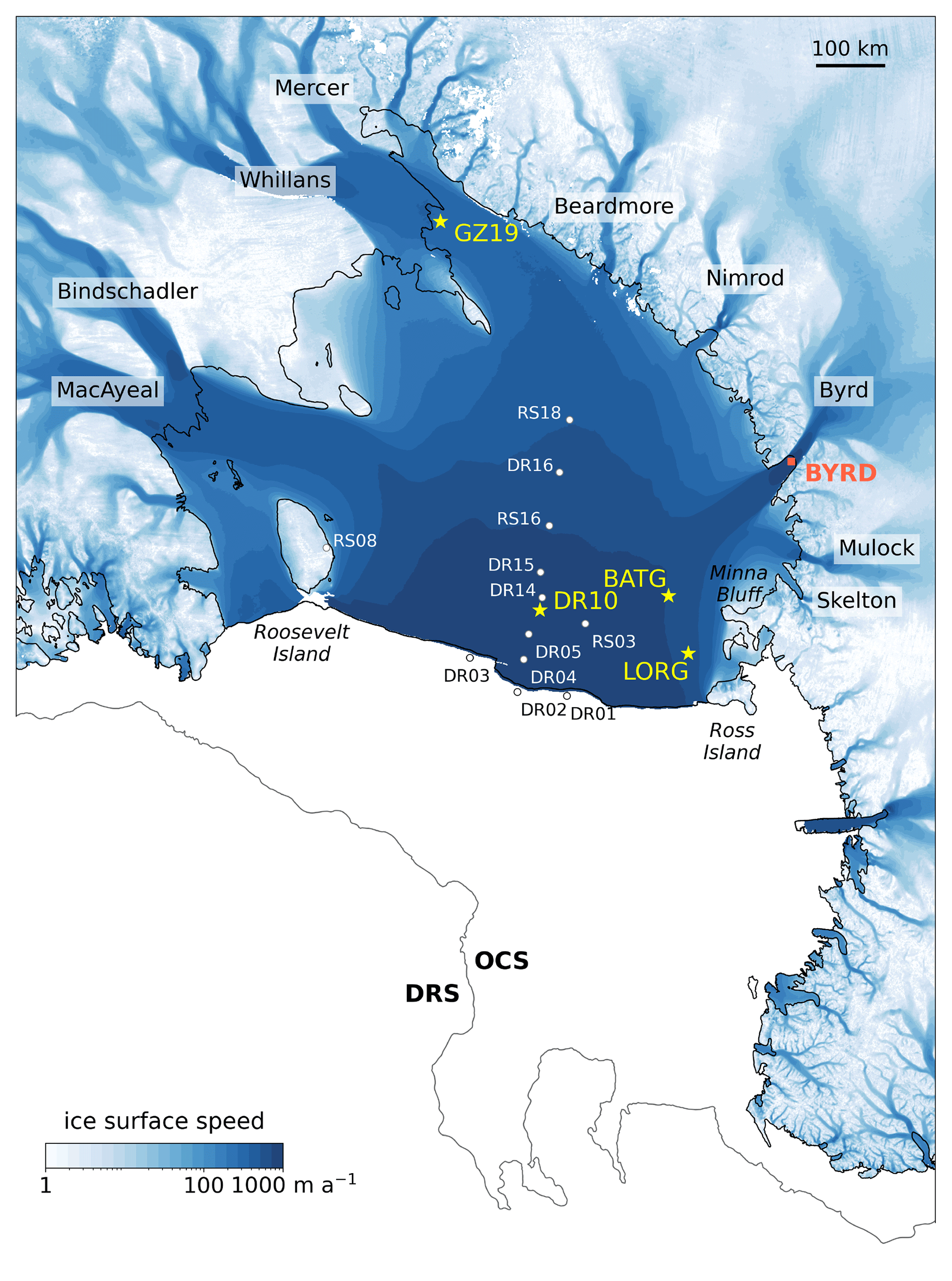
Figure 1Map of the Ross Ice Shelf and its surrounding principal outlet glaciers and ice streams. The locations of GNSS stations used in this study and their names are indicated; see Table 1 for more details. Our focus is on long time series from DR10, BATG, LORG, and GZ19 (yellow stars). BYRD (orange square) is not a GNSS site but identifies the area analysed in Fig. 9e. The background image shows time-averaged surface velocities measured by satellites (Rignot et al., 2017). The grounding line and the ice front, from Depoorter et al. (2013), are plotted with black lines. The 1500 m isobath, separating regions defined as the open continental shelf (OCS) and the deep Ross Sea (DRS), is plotted in dark grey.
2.2 SSH measurements and model estimates
SSH can be estimated using satellite radar altimetry, and monthly SSH estimates are available for the period 2011–2016 for regions north of the Antarctic coastline and ice shelves using measurements from the European Space Agency's CryoSat-2 radar altimeter (Armitage et al., 2018). These SSH estimates cover fully open water (free of ice shelves) and leads in the ice pack but do not extend under the ice shelves. Measuring SSH variations in the ocean cavities under ice shelves is challenging because they are small compared with other contributors to height changes, such as uncertainties in seasonal cycles of basal mass balance (e.g. Stewart et al., 2019; Tinto et al., 2019), snow and firn density changes (e.g. Zwally and Jun, 2002; Arthern and Wingham, 1998), and penetration of radar signals into the surface snow and firn layers (Ridley and Partington, 1988; Davis and Moore, 1993). Therefore, it is not currently possible to accurately estimate SSH variability under ice shelves.
Instead, we investigated the representation of intra-annual variability in SSH from five existing ocean models with thermodynamically active ice shelves (Mathiot et al., 2017; Tinto et al., 2019; Naughten et al., 2018; Dinniman et al., 2020; Richter et al., 2022). We used their SSH output relative to the Armitage et al. (2018) open water data set to determine the most realistic model for analyses and to assess the likely variability in SSH under ice shelves. More information on these models, and assessment of their performance, is provided in the Supplement. From these analyses we determined that the Ross Sea regional model described by Tinto et al. (2019) provides a seasonal cycle that is most consistent with the Armitage et al. (2018) satellite-based results for the Ross Sea continental shelf north of RIS, suggesting that it is also the best model for SSH variability under RIS.
2.3 Ice sheet/ice shelf model
2.3.1 Model summary and initialisation
We used the open-source ice sheet and ice flow model Elmer/Ice (Gagliardini et al., 2013), the glaciological extension of the Elmer finite-element software developed at the Center for Science in Finland (CSC-IT). The modelling framework is similar to that described by Klein et al. (2020). We added variability in SSH in both time and space, relative to the initial static sea level, focusing on SSH output from the Tinto et al. (2019) ocean model as justified in the Supplement. Our ice model uses the vertically integrated shallow-shelf approximation (SSA; MacAyeal, 1989), a simplification of the Stokes equations (usually used for resolving viscous flow problems) in which the ice velocity is considered constant throughout the ice thickness. This approximation is well suited to ice shelves and ice streams where vertical shear stresses are negligible relative to other stresses acting on the ice. The ice rheology is based on a nonlinear constitutive relationship between strain rates and deviatoric stresses, classically used in ice flow modelling and known as Glen's flow law (Glen, 1958). The shear stress at the ice–bed interface, τb, is modelled with a Weertman friction law (Weertman, 1957) at the ice–bed interface:
with C being the friction coefficient, ub the sliding velocity, and exponent where increasing values of m are characteristic of a more plastic bed. We use a value m=1 in this study and discuss this choice in Sect. 4.1.
Following the same procedure used by Klein et al. (2020), we initialised our model by inferring the basal shear stress (on grounded ice) and the ice viscosity, using an inverse model that optimises the two parameters by minimising the difference between the model and observed surface ice velocities as well as the difference between ice flux divergence and observed mass balance. Details on the model setup can be found in Appendix A1.
There are two main effects of SSH variability on the ice shelf velocities: (i) changes in driving stress and (ii) changes in basal stress through grounding line migration.
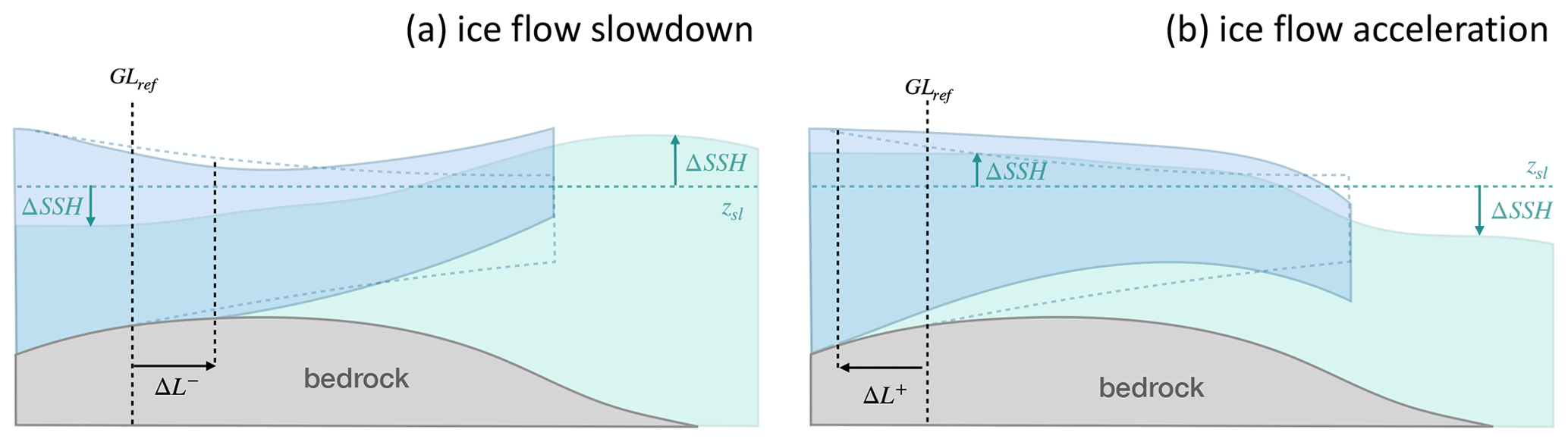
Figure 2Conceptual model of the SSH effect on the ice shelf slope and grounding line position: combination of (a) a positive ice shelf tilt and a negative ΔSSH close to the grounding line and (b) a negative ice shelf tilt and a positive ΔSSH close to the grounding line. The average annual state of the ice shelf is shown by dashed lines, while the perturbed state is shown by plain lines. The combinations shown are for seasonal velocity changes from grounding line migration and tilt being roughly in phase as suggested by SSH models for RIS (see Fig. 4).
- i.
Driving stress change.
Changes in gradients of SSH locally impact the driving stress, σg (in MPa), acting on the ice flow. This stress is a direct function of the surface gradient, ∇zs, with zs being the ice shelf surface height (assuming solid ice from the surface to base) relative to the background unperturbed sea surface, following, for example, Morland (1987), MacAyeal (1989), and Gudmundsson (2013):
In Eq. (2), ρice is the density of ice (917 kg m−3, assumed constant over the ice thickness), g is the gravitational acceleration (9.81 m s−2), h(xyt) (m) is the ice shelf thickness, and ΔSSH(xyt) is the SSH perturbation. A decrease in the ice shelf seaward gradient leads to a decrease in driving stress and a deceleration in the ice flow (Fig. 2a). An increase in the ice shelf seaward gradient leads to an increase in driving stress and an acceleration in the ice flow (Fig. 2b).
- ii.
Change in basal stress through grounding line migration.
SSH variations lead to changes in bed stresses in the grounding zone, as they raise and lower the ice shelf and influence the subglacial hydrology near the grounding line. A negative ΔSSH at the grounding line causes a downstream migration of the grounding line, increasing the grounded-ice area and potentially slowing down ice movement through an increase in basal drag (Fig. 2a). Conversely, a positive ΔSSH at the grounding line leads to an upstream migration of the grounding line, decreasing the area affected by basal stresses and accelerating the ice flow (Fig. 2b). The grounding line migration distance (ΔL) upstream and downstream is influenced by viscoelastic deformation of the ice shelf. The mechanism has been studied in the context of tidal deformation by treating it as an elastic and hydrostatic beam problem (e.g. Sayag and Worster, 2011, 2013; Walker et al., 2013). This analytical solution agrees reasonably well with grounding line migration calculated by solving the contact problem in a viscoelastic, tide-forced model (Rosier et al., 2014).
In a purely hydrostatic framework, the grounding line migration (ΔL) depends on both the surface and bed slopes (Eqs. B7 and B8; Appendix B) (Sayag and Worster, 2014): as surface and bed slopes decrease, ΔL increases. This inverse relationship directly affects the magnitude of the change in friction in the grounding zone and also the ice flow response. The implications of uncertainties in our knowledge of bed slope and ΔL and the mechanical processes involved are discussed further in Sect. 4.2.
Grounding line migration ΔL has also been treated as an elastic fracture problem, accounting for water pressure variations at the ice base as the grounding line migrates. Using this framework, Tsai and Gudmundsson (2015) showed that the magnitude of upstream ΔL is larger than in the hydrostatic or purely elastic case and depends nonlinearly on parameters such as the ice thickness and ΔSSH. For thick ice (e.g. in the grounding zone of Byrd Glacier), ΔL can be more than twice the value obtained using the hydrostatic framework, and for small ΔSSH (typically, a few centimetres), ΔL can be as much as 1 order of magnitude higher than in the hydrostatic framework.
2.3.2 Model runs
We ran 100 inversions of both the basal friction and the ice viscosity, constraining the fit to velocity and thickness rate of change observations, as well as the degree of smoothness of the solution. The set of inversions explores the effect of each constraint by varying their respective weight. From this ensemble of initial states, we selected an optimal (in terms of velocity and ice flux divergence fit) sub-ensemble of 15 members (Ω15). The details of the initialisation procedure and the selection of Ω15 are discussed in Appendix A1.
Using the sub-ensemble Ω15 as a reference, we applied monthly averaged SSH anomalies (ΔSSH) from five different ocean models (see Supplement) as a steady-state perturbation, raising or lowering the ice surface, and ice base and computing the flow change with respect to the reference (see Appendix A2). For each run, we kept the ice shelf thickness constant and assumed that the ice shelf and the grounding line location adjust instantaneously to the ΔSSH.
To assess the importance of methods for representing grounding line migration in our viscous ice sheet model, we ran three different parameterisations of ΔL (for a total of 225 simulations =15 members × 5 SSH models × 3 grounding line parameterisations), as follows:
-
ΔLB2 is based on the hydrostatic equilibrium of the grounding line and Bedmap2 (a gridded product describing surface elevation, ice thickness, and the basal topography of the Antarctic; Fretwell et al., 2013) bed slopes at the grounding line.
-
ΔLC (constant bed slope) is a significantly larger migration that corresponds to values used by Rosier and Gudmundsson (2020) for their study of the Filchner–Ronne Ice Shelf when treating the grounding line migration with elastic fracture mechanics introduced by Tsai and Gudmundsson (2015).
-
ΔLB2L is also a larger value of grounding line migration but accounting for the Bedmap2 surface and bed slope variations along the grounding line.
To account for subgrid-scale migration of the grounding line, our model implementations parameterise ΔL as a change in friction, rather than as a change in floatation state at specific grid nodes (Appendix B). The implications of the two larger migration parameterisations are discussed in more detail in Sect. 4.2.
We first review the intra-annual variability in ice flow recorded by the GNSS receivers on RIS (Sect. 3.1.1) and the measured (Armitage et al., 2018) and modelled (Tinto et al., 2019) seasonal cycles of SSH for the Ross Sea including under RIS (Sect. 3.1.2). We then compare the variability in driving stresses due to SSH anomalies and grounding line migration (Sect. 3.2) and the effect of both processes on the ice speed flow (Sect. 3.3).
3.1 Intra-annual signals in GNSS displacement and SSH records
3.1.1 GNSS displacement
All long-duration GNSS stations on RIS (Sect. 2.1) show variability in horizontal displacement on various timescales including diurnal (∼1 d period), fortnightly (∼2-week period), and intra-annual (Fig. 3). As reported by Klein et al. (2020), data from the DRRIS stations show evidence of an annual cycle with a displacement anomaly amplitude of about 1 m, alternating between a negative trend during December–May and a positive trend during June–November. GZ19 shows no apparent annual cycle, but its displacement shows a similar range of variability (±1 m) to DR10 during the 2-year record. The time series at BATG, which is not concurrent with the DRRIS stations and GZ19, shows a smaller amplitude range (about 0.2–0.3 m) that appears to have a periodicity of about 6 months. The LORG time series in 2019 shows a similar pattern to BATG in 2018.
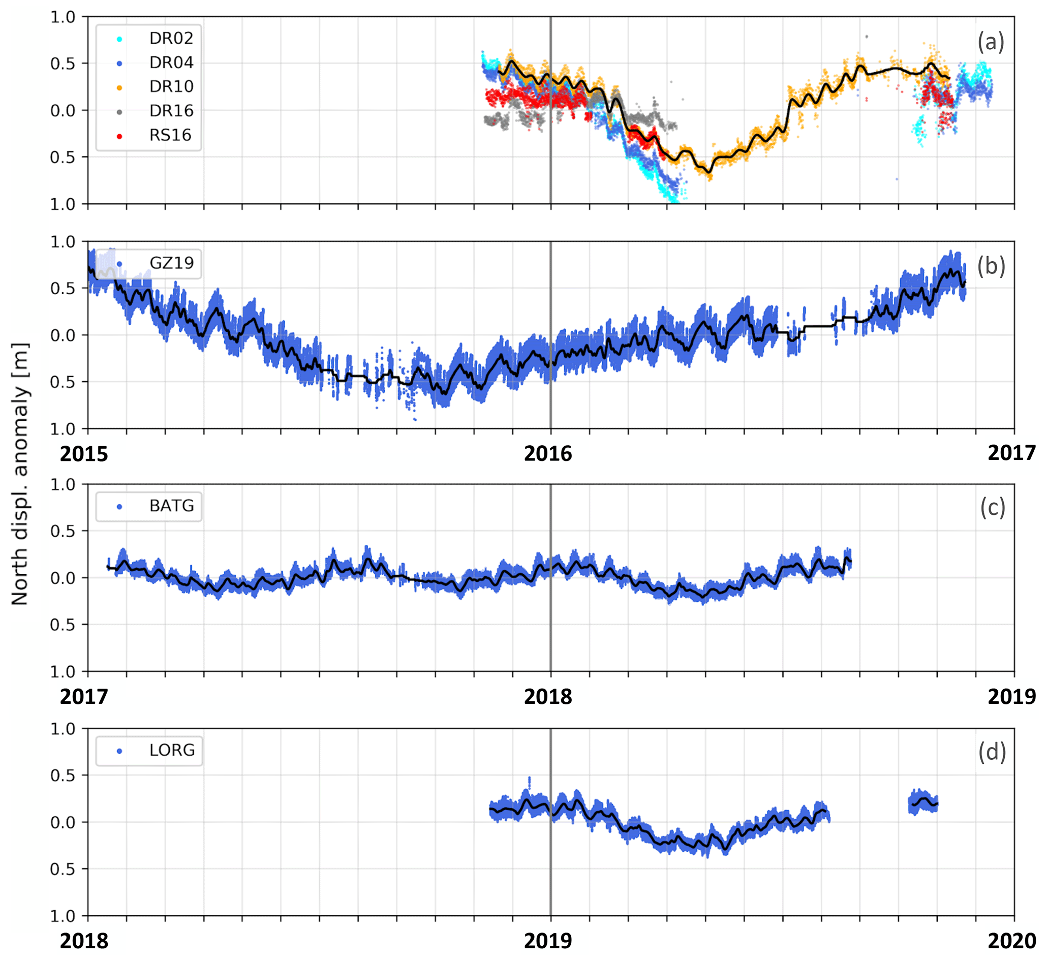
Figure 3GNSS horizontal displacement anomalies in the north direction (approximately parallel to the time-averaged flow) for GNSS stations used in this study. The time interval for each panel is 2 years; however, years differ between panels. (a) DR02, DR04, DR10, DR16, and RS16 (for legibility, other DRRIS sites are not shown here but exhibit a similar trend; the complete array can be found in Klein et al., 2020); (b) GZ19; (c) BATG; and (d) LORG. Note that (a) and (b) are plotted on the same timescale, while (c) and (d) have 2-year and 3-year shifts with respect to the two upper panels. The black lines are smooth versions of displacement anomalies with a 1 d Gaussian RMS width.
The diurnal lateral displacement signal is caused by the fundamental tides of the region, which are almost entirely diurnal (e.g. Padman et al., 2003; Ray et al., 2021). We attribute the fortnightly signal in displacement at all GNSS sites (and, possibly, also the ∼6-month periodicity at BATG and LORG) to nonlinear response of the ice sheet and ice shelf to variability in the tidal range, leading to viscoelastic flexural adjustments of the ice sheet at the grounding zone, as the range of the diurnal tide varies through the fortnightly spring–neap modulation (e.g. Rosier and Gudmundsson, 2020). We removed the fortnightly tide-forced variability by filtering to monthly and longer timescales (by using a sliding Gaussian filter with a 2-week standard deviation); however, any ∼6-month tidal signal remains as a source of noise in our interpretation of intra-annual ice shelf flow changes driven by non-tidal SSH variability.
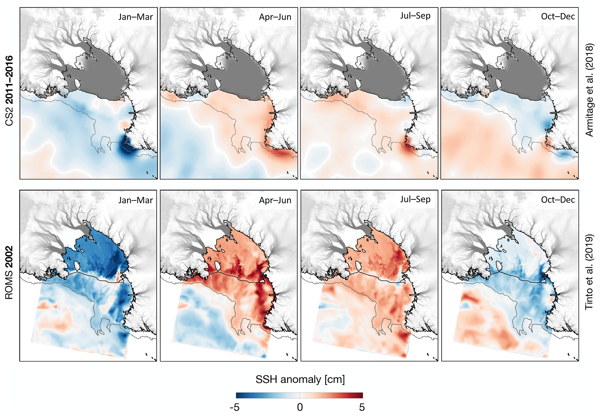
Figure 4Seasonal sea surface height deviation from the annual mean (ΔSSH): (top row) satellite observations averaged over the period 2011–2016 (ΔSSHCS2, Armitage et al., 2018) and (bottom row) modelled for the period 2002 (SSH2002, Tinto et al., 2019). The ice front and grounding line are represented by black lines. The outer edge of the open continental shelf (OCS) is along the 1500 m isobath, shown with a grey line. Ice speeds are shown in shades of grey, with darker shades being faster.
3.1.2 Satellite-derived and modelled SSH
The seasonal cycle of ΔSSH in satellite-derived SSH fields around Antarctica, for the period 2011–2016, shows a typical range of about 5 cm on the open continental shelf (OCS; see Fig. 1) of the Ross Sea and comparable changes offshore in the Deep Ross Sea (DRS); see Fig. 4, top row, and Fig. 5. For the OCS, a positive SSH anomaly occurs in winter (April–September). The Tinto et al. (2019) model, based on annually repeating forcing for 2002, shows similar phasing of the ΔSSH cycle (Fig. 4, bottom row; Fig. 5a) but with larger amplitude than for the satellite-derived fields. The qualitative and quantitative (see Table S2 of Pearson correlation coefficients of the different models) agreement between the model and the observations offshore of RIS provides support for the use of this ocean model for predicting SSH variability under RIS, even though the ocean model does not overlap in time with either the observed SSH fields or the GNSS observations.
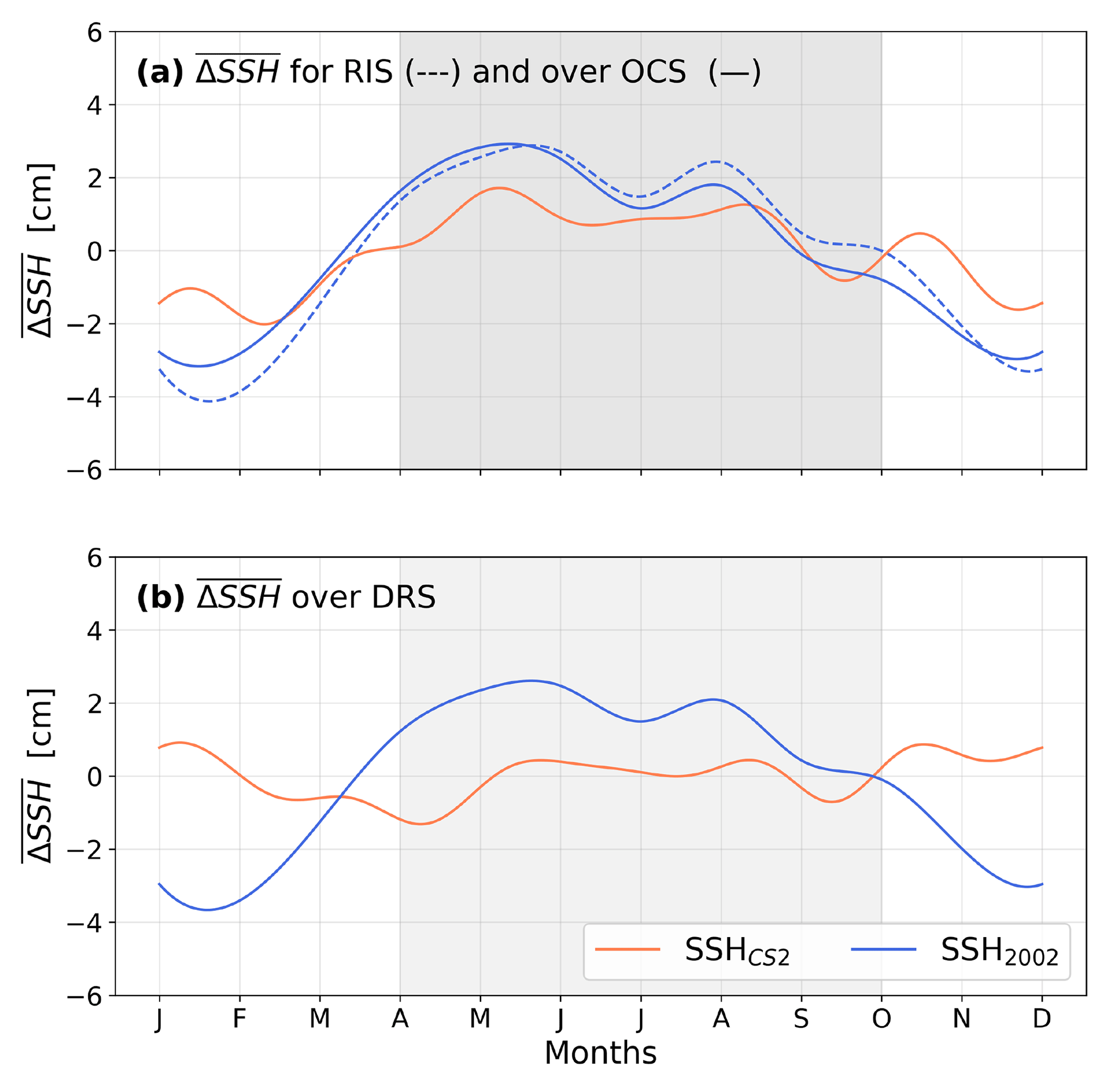
Figure 5(a) Annual cycle of monthly mean ΔSSH over the open continental shelf (OCS – plain lines) and beneath the ice shelf (RIS – dotted lines) for SSH2002 (blue) and for CryoSat-2 measurements (SSHCS2, red) averaged over 2011–2016, for the open continental shelf (OCS) only. (b) Mean ΔSSH for the deep Ross Sea. The grey shade shows the winter period. See Fig. S3 for similar comparisons that include all available ocean models of SSH.
3.2 Comparing driving stress change and grounding line migration
RIS thickness decreases from ∼800 m close to the grounding line to ∼300–400 m at the ice front, over a distance of ∼800 km (see Tinto et al., 2019, their Fig. S2a). This results in mean thickness and surface gradients of about and , respectively. Since we are interested primarily in along-flow variations in ice velocity, we calculate the along-flow Lie derivatives (Yano, 2020) of the ice shelf surface height () and ΔSSH (). Values of range from 10−5 to 10−2 over most of the ice shelf (Figs. 6a and S4a). Gradients of ΔSSH in Tinto et al. (2019; SSH2002) can reach 10−6 to 10−5 in February (Figs. 6b and S4b). This means that local tilting of the ice shelf by can modify the local driving stress of the ice shelf (Eq. 2) typically by 0.1 %–1 % and sometimes up to several percent, with substantial spatial variability (Fig. 6c). also varies by month (not shown). For example, in February, about 30 % and 6 % of the ice shelf experiences a fractional change of driving stress exceeding 0.1 % and 1 %, respectively (Fig. 6d). The largest fractional change in driving stress occurs away from the grounding line where the ice surface height gradients are smaller than closer to the grounding line and where the SSH gradients are the larger.
The complex spatial variability of the along-flow derivatives of ΔSSH (Fig. 6b) arises from changes in orientation and magnitude of the sub-ice-shelf circulation relative to ice flow. This circulation is itself complex: see, for example, Supplementary Video 1 in Tinto et al. (2019).
For most months there is a strong along-flow gradient in SSH close to the ice front (Figs. 4b and 6b), which directly impacts driving stress (Eq. 2). These variations in driving stress lead to ice velocity changes, which we present as anomalies with respect to the annual average velocity field. In general, months with a regionally averaged (i.e. over the ice shelf) negative ΔSSH (e.g. January–March period in Figs. 4 and S2) that slows ice flow as the grounding line migrates seaward also experience a relative uplift of the surface close to the ice front, leading to an additional slowdown (Fig. 2a). Conversely, the months experiencing a regionally averaged positive ΔSSH generally show a relative surface drop close to the ice front and an upstream migration of the grounding line, both contributing to an acceleration of the ice shelf (Fig. 2b).
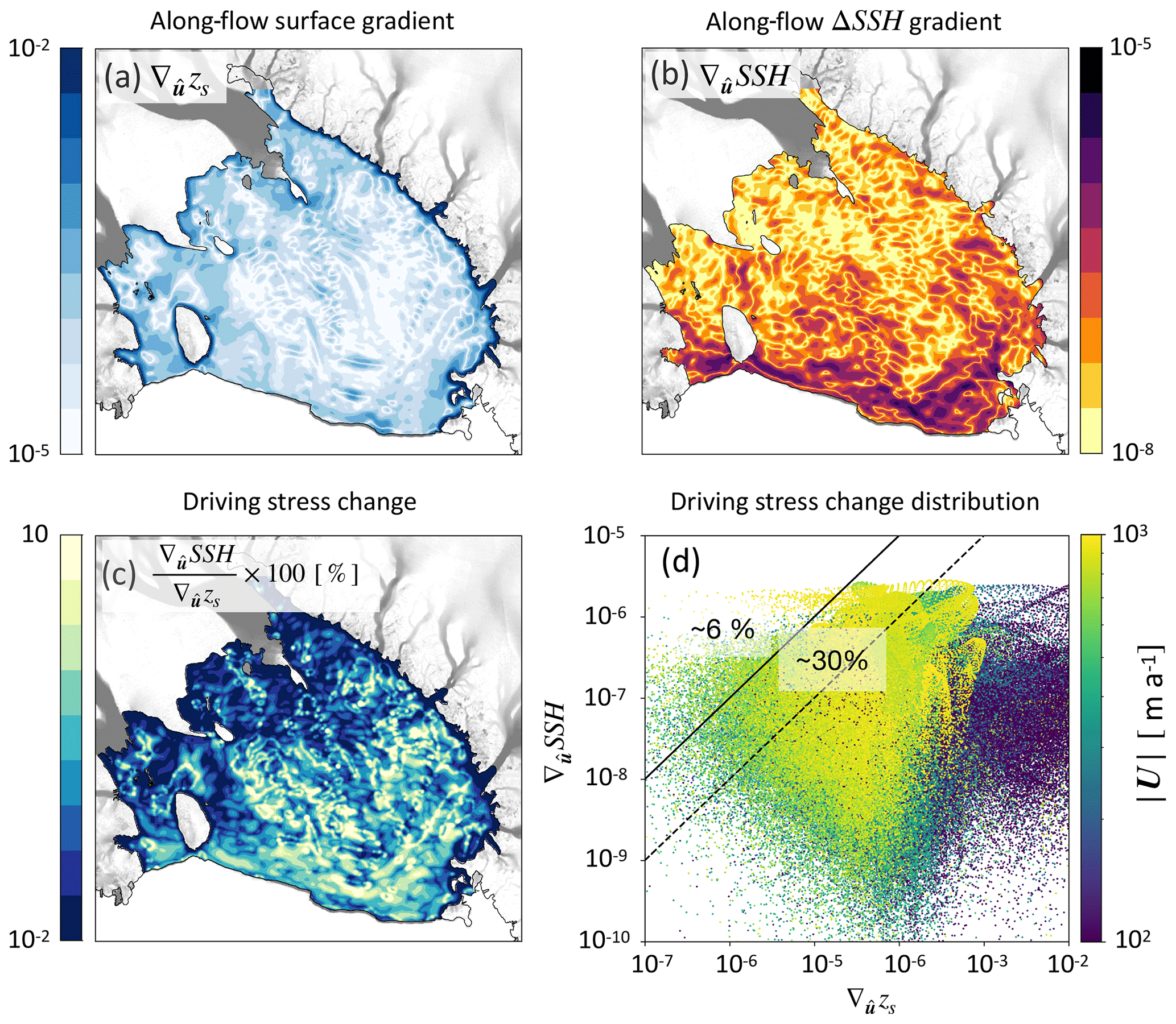
Figure 6Comparison of ice shelf surface gradients and SSH gradients from SSH2002 (Tinto et al., 2019), both calculated in the direction of ice flow () in February. (a) Ice shelf surface gradient (), (b) SSH gradient (), and (c) their ratio. Gradients are filtered with a 5 km standard deviation Gaussian smoothing. (d) Gradient values, for each 1×1 km cell, plotted as a function of each other. The colour map represents the ice flow speed. A total of 6 % and 30 % of the model nodes over the ice shelf experience a driving stress variation of more than 1 % (left of the plain line) and 0.1 % (left of the dashed line), respectively.
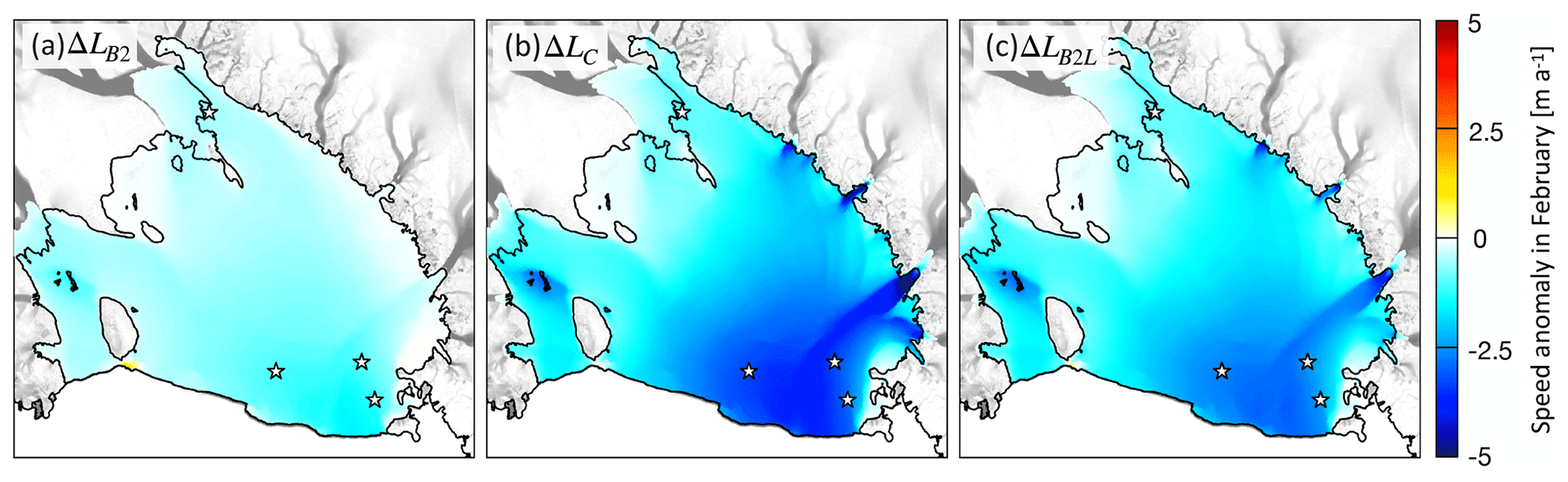
Figure 7February anomaly in velocity ΔU, averaged over an ensemble of 15 initial states (Ω15), formed as the difference between the annual average for ΔSSH2002 and the three different parameterisations of the grounding line migration: (a) ΔLB2, (b) ΔLC, and (c) ΔLB2L (see Sect. 2.3.2). The locations of DR10, GZ19, BATG, and LORG (identified in Fig. 1) are indicated by white stars. The grounding line and the ice front are shown by black lines. The background annual average flow velocity for grounded ice is plotted in shaded grey, with darker grey being faster.
Our modelling indicates that the amplitude of the grounding line migration, ΔL, is the primary control on the amplitude of the seasonal velocity signal. In February, for example, the model ensemble using ΔLB2predicts the smallest amplitude of velocity deviation of the three cases, with m a−1 over most of the ice shelf (Fig. 7a). Larger values of ΔL (parameterisations ΔLC and ΔLB2L) allow the grounding line to move farther downstream during summer, leading to deviations m a−1 in the centre of the ice shelf (Fig. 7b and c). The largest differences between the effects of ΔLC and ΔLB2L are generally found close to the grounding line in the deep and narrow fjords such as the floating extension of Byrd Glacier where ΔLC leads to a slowdown ΔUC<5 m a−1 compared with ΔUB2L∼3 m a−1 (Fig. 7b and c). These are regions where true bed slopes are steeper than the average around the RIS perimeter and which are also more sensitive to the initial state as the ensembles show a larger standard deviation in these areas with respect to the rest of the domain (Fig. 8, bottom row).
We regard the ΔLB2 parameterisation, which yields small grounding line migration, as an approximation of ice shelf response to SSH gradients alone.
3.3 Seasonal cycle in ice flow
All ensembles forced with ΔSSH2002 exhibit a maximal seasonal negative flow speed anomaly during summer and maximal positive anomaly during winter (Fig. 8); however, ΔLB2 simulations tend to switch to positive anomalies later than simulations using ΔLC and ΔLB2L. Simulations using ΔLB2 produce maximal amplitudes of speed anomaly at the ice front that progressively decrease farther upstream, while ΔLC and ΔLB2L produce maximal speed anomaly amplitudes in the deep fjords along the base of the Transantarctic Mountains. The amplitudes of speed anomalies of ΔLB2 are about 2–4 times smaller than for ΔLC and ΔLB2L simulations, depending on location.
To validate the results of the three grounding zone parameterisations, we extracted the modelled ice velocity anomalies at the GNSS locations and compared these to velocity variations (Fig. 9) estimated from the time derivative of measured displacement anomalies (Fig. 3).
At DR10, the range of the observed velocity anomaly (ΔU) was about 10 m a−1 with a minimum in February–March and a maximum in July (Fig. 9a). The other DRRIS GNSS stations located in the centre of the ice shelf did not record during austral winter (see Fig. 5a), preventing us from properly identifying the timing of maximum velocity for these stations. The ΔLC and ΔLB2L ensembles both give similar ΔU estimates that are qualitatively similar to observations, with velocity variations of about 50 % to 70 % of the observed amplitude and minima and maxima in summer and winter, respectively. The ΔLB2 grounding zone parameterisation has a much lower amplitude than observations and gives a maximum velocity in October, about 2 months later than the other ensembles and 4 months later than the observations. However, the timing of the summer ΔU minimum is close to the observations and the other grounding zone parameterisations. Expanding our analysis to the entire GNSS array of DRRIS, similar seasonal phasing occurred at each GNSS station located approximately along the central flowline of the ice shelf. ΔU amplitude generally decreases with increasing distance from the ice front (Fig. 10), although with some variability that may result from the proximity of the DRRIS array to the Byrd Glacier flow and its impact on RIS flow.
At GZ19, close to the grounding line of Whillans Ice Stream, there is no seasonal cycle visible in the GNSS observations of displacement anomaly (Fig. 3b). The measured velocity anomaly (Fig. 9b) shows an overall slowdown, consistent with previous observations of slowdowns of Whillans and Mercer ice streams and the adjacent region of RIS over the last few decades (e.g. Joughin et al., 2005; Thomas et al., 2013), and shorter periods of deceleration and acceleration that could be due to the inherent variability in the two ice streams (e.g. Winberry et al., 2009). This trend was not captured by our ice flow models, which do not account for varying forcing other than the annual cycle of SSH. The modelled anomalies at GZ19 are weak, with m a−1 and m a−1 over the year.
At station BATG, about 100 km east of Minna Bluff, the velocity time series shows an approximately 6-month periodicity, with a ΔU range of about 2.5 to 3 m a−1 (Fig. 9c). ΔLB2 provides a poor fit to these observations, in both ΔU amplitude and phase, with the amplitude better reproduced by ΔLC and ΔLB2L. However, the pattern of observed velocity anomaly changes between the first and second year of the record. In the first year, the 6-month cycle shows a large velocity drop in July–August (reaching a minimum in September), corresponding to the second minimum of the year. In the second year, the observed velocity reached a maximum in May and remained relatively high until the end of August, fitting the modelled velocities. While the record terminated at the end of August, this marked a particularly long plateau of high velocities (from May to August), suggesting that the record includes a seasonal signal that is added to the 6-month cycle that we tentatively attribute to semiannual changes in tidal range (see Sect. 1).
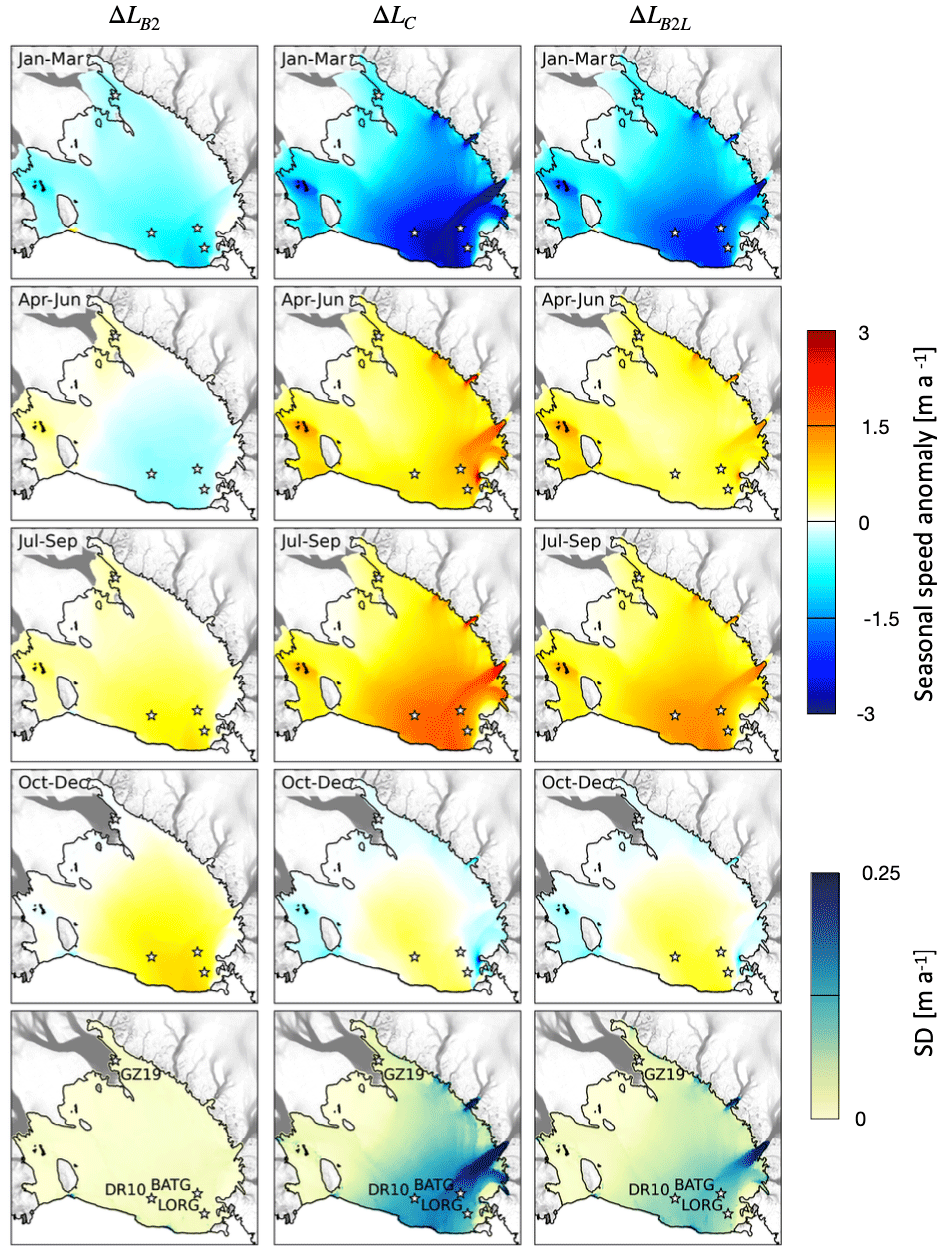
Figure 8Ensemble mean seasonal (3-month average) ice flow anomaly for ΔSSH2002 and three parameterisations of the grounding line migration: (first column) Bedmap2 (ΔLB2), (second column) a constant bed slope (ΔLC), and (third column) a flatter version of Bedmap2 (ΔLB2L). The seasonal anomalies are computed from monthly model outputs. The standard deviation over the ensembles (bottom row) shows variability in space and time over the year. The locations of DR10, GZ19, BATG, and LORG are indicated by white stars. The ice front and the grounding line are indicated by the black line. Ice surface velocities over the grounded ice are plotted with a grey scale, from white (slow flow) to dark grey (fast flow).
Figure 9Comparison between GNSS and model velocity anomaly when applying ΔSSH values from SSH2002 for (a) DR10, (b) GZ19, (c) BATG, and (d) LORG and (e) at the Byrd Glacier outlet (see locations in Fig. 1). The annual model cycle is repeated over 2 years. The average model velocity anomalies (over Ω15 ensembles) – ΔUB2 (grey), ΔUC (red), and ΔUB2L (blue) – are displayed with 1 and 2 standard deviations of the 15 estimates in each ensemble (dark and light shades, respectively). If not visible, the standard deviation is statistically insignificant. ΔUB2, ΔUC, and ΔUB2L are plotted from monthly time series with a continuous line drawn between each snapshot. In (b), ΔUC (red) and ΔUB2L (blue) are so similar that we cannot distinguish them. The observed velocities (green) are obtained as the time derivative of the measured displacement anomaly (the period of observation is given in green in each panel) from GNSS, with a Gaussian filter with a 2-week standard deviation. See Fig. S6 for similar comparisons that include all available ocean models of SSH.
The time series of ΔU at LORG (Fig. 9d) for the period November 2018 to November 2019 is highly correlated (p=0.95) with the time series at BATG over the second year (from November 2017 to October 2018). The predicted velocity anomalies for ΔLC and ΔLB2L at these two stations agree especially well with the observations over the entire LORG times series and the second year of the BATG time series. More specifically, the model is able to reproduce the month-to-month accelerations and decelerations and the overall longer span of positive anomalies visible in LORG observations.
To examine the relative effect of the variations in driving stress and basal friction through grounding line migration, we consider a key region of RIS, the floating extension of Byrd Glacier near its grounding line. Byrd Glacier is the fastest and the deepest outlet glacier feeding RIS and is the region of RIS where the outputs from the three ensembles (ΔLB2, ΔLC, and ΔLB2L) deviate the most. Observations show that, over a time span of a few years, flow upstream of the grounding line can increase by 10 %, coinciding with the discharge of subglacial lakes lubricating the bed (Stearns et al., 2008; Yuan et al., 2023). At seasonal timescales, variations in Byrd Glacier remain poorly constrained due to the lack of year-round GNSS measurements; however, Greene et al. (2020) used feature tracking in satellite imagery to estimate ice velocities and characterise the magnitude and timing of seasonal ice dynamic variability. For a region close to the grounding line of Byrd Glacier, they estimated seasonal variability of ΔU with a range of roughly 45 m a−1. Our ensemble using the ΔLB2L representation (Fig. 9e) shows a phase that is consistent with Greene et al. (2020); however, our modelled range in ΔU is always less than 10 m a−1. This difference could be explained by the substantial uncertainty due to irregular, seasonally biased sampling of the satellite data (see Fig. 4 of Greene et al., 2020). Our modelling may also underestimate either the ΔSSH or the basal condition changes that the ΔSSH changes trigger. There may also be other processes at play that we do not account for in our modelling; for example, the change in seasonal melt (explored in Klein et al., 2020) which, while expected to be small, could slightly increase the ΔU signal.
Our ice sheet modelling results suggest that seasonal variations in SSH beneath RIS are sufficient to drive ice velocity variations of several metres per year over a large portion of the ice shelf when using the ΔLC and ΔLB2L parameterisations to represent basal stress change in the migrating grounding zone. The modelled velocity variability generally decreases with increasing distance from the ice front, although large variability is also associated with several major outlet glaciers flowing through the Transantarctic Mountains. However, the correlation between model and GNSS observations depends on the model initialisation, friction law, grounding line parameterisation, and the source of the SSH forcing. In this section, we discuss the sensitivity of the model and the uncertainty of each of these parameters.
4.1 Model initialisation and friction law
The inverse model used to generate the initial steady-state solution is under-constrained. Because we infer two parameters with multiple constraints during the inversion, an initial state with a minimal velocity misfit will not necessarily lead to a minimal ice thickness rate of change. Different combinations of friction and viscosity parameters can lead to similar misfits. Using the ensemble Ω15, consisting of the 15 optimal initial states (see Sect. 3.3 and Appendix A1), to estimate the effect of the initialisation on the forward model helps quantify this effect. For the ensemble of simulations using the ΔLB2 parameterisation, the impact of the initial state on the velocity intra-annual cycle is minimal over the ice shelf, with an average relative standard deviation under ∼5 % over most of the ice shelf (Fig. 8 (bottom row) and Figs. 9 and 10). The ensemble responses for the ΔLC and ΔLB2L parameterisations, while providing more realistic estimates of intra-annual velocity changes, show more sensitivity to the initial state with year average relative standard deviations of ∼15 %–20 % (±0.1–0.15 m a−1) at DR10 and ∼25 % (±0.4 m a−1) at Byrd Glacier. We attribute the relatively high variance of the ensemble in these regions to the sensitivity of the model to the initial basal friction, while the relatively low variance of the ensemble over most of the ice shelf indicates low sensitivity of the model to the initial viscosity parameter.
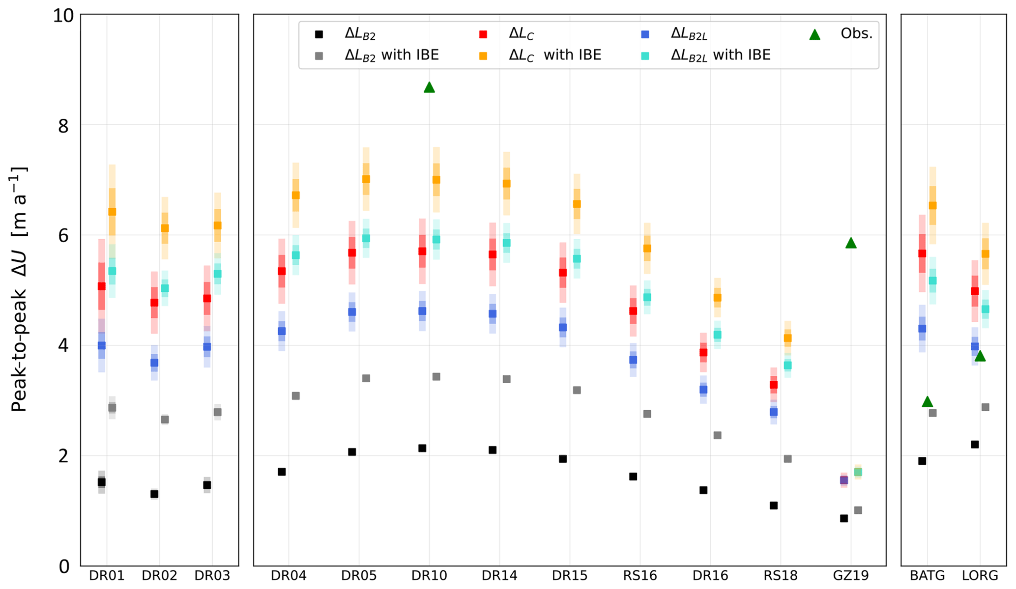
Figure 10Peak-to-peak seasonal range of velocity anomaly (ΔU) when forcing the ice flow model with ocean model ΔSSH2002. The error bars (in shades) correspond to 1 and 2 standard deviations in each ensemble. Observed peak-to-peak range is also plotted for GNSS stations with data records longer than 1 year (i.e. DR10, GZ19, BATG, and LORG).
The friction law used in the model will also influence ice flow response, even for the same value of ΔL. Friction laws of different complexity have been proposed in the literature (Weertman, 1957; Budd et al., 1979; Schoof, 2005; Tsai et al., 2015) and have been shown to have different impacts on grounding line dynamics (e.g. Brondex et al., 2019). In our study, we only used the most common friction law (Weertman, 1957).
The results described in Sect. 3.2 were obtained with a linear version (m=1) of Eq. (1); i.e. stress is proportional to velocity. We also tested the value m=3 (e.g. Brondex et al., 2019; Gudmundsson et al., 2019), which only changes modelled velocity anomalies by a few percent. More complex friction laws (e.g. Schoof, 2005; Tsai et al., 2015; Joughin et al., 2019) that include the impact of water pressure change at the ice base as the grounding line migrates could increase the amplitude of our intra-annual velocity variations. However, such friction laws introduce additional poorly constrained parameters (Gillet-Chaulet et al., 2016) and, therefore, are not considered in this study.
4.2 Grounding line migration and basal stress change
The parameterisation of ΔL directly controls the amplitude of the grounding line migration which, in turn, controls the change in the friction coefficient we apply at the grounding line (see Sect. 3.3 and Appendix B). ΔLB2 leads to small migration of the grounding line (typically a few metres) so that most of the impact of SSH variability on the ice flow comes from changes in ΔSSH gradients. While driving stress variations from these SSH gradients and small grounding line migration (ΔLB2) due to ΔSSH can slow down or accelerate the ice flow by about ±1 m a−1 (Figs. 6 and 7), these modelled variations are only ∼20 % of the observed ΔU at DR10. Incorporating a larger grounding line migration in the model (ΔLC and ΔLB2L) gives values of ΔU that are consistent with our GNSS observations. Such grounding line migrations with respect to the hydrostatic case (ΔLB2) are, arguably, too strong, but are in line with observations by Brunt et al. (2011) and the values used by Rosier and Gudmundsson (2020) on the Filchner–Ronne Ice Shelf. The surface and bed slope are key parameters of the grounding line migration parameterisation (Tsai and Gudmundsson, 2015; Appendix B). The bed slopes around the RIS perimeter, estimated by Brunt et al. (2011) by applying the hydrostatic assumption to observed migration of the inner margin of tidal ice flexure in repeat-track satellite altimetry, are likely to be biased low, based on the modelling of Tsai and Gudmundsson (2015). While the ΔL values given by ΔLC and ΔLB2L are in the upper range, they remain consistent with previous studies of tidal migration of the grounding line.
Another explanation for our need for a large migration of the grounding line is the relatively low value of the basal friction coefficients we inferred at the grounding line during the model initialisation. Our initialisation scheme relies on the optimisation of the friction coefficient C in Eq. (1). This friction law does not include a direct dependency on the effective pressure as a Coulomb law would (e.g. Brondex et al., 2019; Urruty et al., 2022). However, as C is determined by inversion, it includes a dependency on the effective pressure close to the grounding line and reduces the value of C at the grounding line to match observations of velocity and thickness rate of change (e.g. Urruty et al., 2022). The inferred value represents an average annual value of the friction coefficient. The distribution of the seasonal variation around this annual average cannot be exactly determined without proper knowledge of the subglacial hydraulic system, but one can assume that the variation could be larger than the variations we estimate through our hydrostatic parameterisation (i.e. a change in C directly proportional to ΔL). Seawater intrusion at the ice–bed interface and in sediments has been shown to have a high impact on the ice flow response (e.g. Robel et al., 2022). Subglacial models depending on subglacial water pressure decrease effective pressure significantly near the grounding line, leading to an increased sensitivity for a given power in the sliding law (e.g. Kazmierczak et al., 2022). Seawater intrusion could also be enhanced by a highly retrograde slope (e.g. Byrd Glacier; see Fig. S6). Retrograde bed slope will enhance both the migration of the grounding line and the intrusion of seawater in the subglacial hydrologic system. The consequences of ΔL on this effective pressure are difficult to determine, but incorporating such a mechanism in our modelling could lead to a larger impact of ΔSSH on the ice flow, even in the purely hydrostatic case.
A final explanation relates to the potential effect of ΔL on the subglacial water system. If the grounding line retreats elastically over a short period, before relaxing to a position closer to the hydrostatic equilibrium, then this short retreat could modify the subglacial water system over a long distance upstream the grounding line. The proper modelling of the water system is largely out of the scope of this study but could help validate our theories in the future.
4.3 Estimating the sea surface height anomalies
The SSH anomalies (ΔSSH) computed in the different ocean models (see Sect. 2.2 and Supplement) result from temporal variability in ocean currents driven by wind stress and lateral density gradients. However, these models do not account for the steric changes due to thermal and haline expansion and contraction or the ocean's response to atmospheric pressure variations. Both the ROMS and NEMO modelling frameworks (see Supplement) use the Boussinesq approximation based on the Navier–Stokes equations: the models conserve volume rather than mass and therefore do not properly account for steric changes. At the same time, variations in atmospheric pressure also lead to isostatic adjustments of the ocean (e.g. Goring and Pyne, 2003), while ice shelves have been shown to respond similarly (Padman et al., 2003). This effect, known as the “inverse barometer effect” (IBE), is not considered in the simulations used in this study. Combining the effect of Boussinesq SSH variations (ΔSSHboussinesq), the steric effect (ΔSSHsteric), and the IBE (ΔSSHIBE), we obtain the total ΔSSH monthly deviation:
Some efforts were made in the 1990s to evaluate the effect of steric sea level due to thermal expansion, concluding that a globally uniform, time-dependent correction of sea level can correct a non-Boussinesq solution (e.g. Greatbatch, 1994). Mellor and Ezer (1995) showed that the seasonal variation in this term is about 1 cm in the Atlantic Ocean, which represents about 10 % of our modelled amplitude of SSH variation over the ice shelf. At the spatial scale of RIS, this correction is roughly spatially uniform and, therefore, would not modify the driving stresses over the ice shelf but could affect the grounding line migration.
Seasonal changes in surface air pressure take place over the Antarctic continent, resulting in a decrease in surface pressure (loss of atmospheric mass) from January to April and an increase in surface pressure (gain of atmospheric mass) from September to December (Parish and Bromwich, 1997). Since most of the ocean models we presented use ERA-Interim reanalysis (Dee et al., 2011) as an atmospheric forcing, we therefore use ERA-Interim surface pressure over RIS to estimate the IBE effect contribution to ΔSSH and its potential effect on the ice flow. ERA-Interim is an older product than the currently recommended ERA5-Land surface air pressure (Hersbach et al., 2020), but both give similar surface pressures over RIS for the period we study, which limits the uncertainty of the IBE effect.
We simulate the effect of IBE on ΔSSH following Eq. (2) and apply the full ΔSSH as a forcing to the ice flow model. Due to the smaller isostatic adjustment of ice shelves to ΔSSHIBE close to the grounding line, we do not include its effect in the grounding line migration. The relative effect of the IBE on the seasonal ice flow is maximal at DR10 and BATG due to their relative proximity to the ocean. In contrast, GZ19 and the region of Byrd Glacier are less affected, since the IBE does not impact grounding line migration (Fig. 10). Overall, accounting for the IBE modifies the peak-to-peak amplitude of ice flow variations by up to ∼1.5 m a−1 (Fig. 10) without significantly impacting the seasonal pattern and phase of the ice flow velocity change. We note that if the IBE was to have a significant impact on the grounding line migration on average, it would most likely increase the amplitude of the grounding line migration with a similar phase to the one we observe without IBE. On a 38-year record of IBE (Fig. S5) the negative inverse barometer signal observed from December to June would lead to downstream migration of the grounding line and a deceleration in the ice shelf flow. Conversely, the positive signal observed from July to November would lead to an upstream migration of the grounding line and an acceleration in the ice shelf flow.
4.4 Ice rheology and timescales
Our ice flow model uses the shallow-shelf approximation (SSA), a viscous rheology, which is well suited for studying long-timescale mechanisms involving ice creep (more than a few days). At the same time, two of our parameterisations of the grounding line migration are based on an elastic rheology, which is more appropriate for short-timescale mechanisms such as tidal effects (less than a few days). In reality, both rheologies are at play but either can sometimes be disregarded with respect to the other, depending on the Maxwell time:
with E being Young's modulus and η the characteristic viscosity of ice. Using a value η∼40 MPa a−1 (obtained from the inferred viscosity parameter and strain rates averaged over the ensemble Ω15 for RIS) and MPa (Cuffey and Patterson, 2010) gives tM∼2 d to ∼2 weeks. Given the seasonal timescale of the variability under consideration in this paper, our viscous ice flow model should adequately represent the real viscoelastic rheology of ice. The elastic migration of the grounding line is, therefore, less representative of the actual viscoelastic rheology for the timescale changes we are observing (SSH anomalies remain relatively stable in periods shorter than a month). However, the elastic parameterisation has previously been successfully applied in a viscoelastic ice flow model studying ice flow response to fortnightly tidal forcing (Rosier and Gudmundsson, 2020). As mentioned in Sect. 4.2., the elastic parameterisation is also a proxy to simulate unrepresented mechanisms that might trigger SSH-induced basal stress change in the grounding zone. Moreover, although the use of an elastic rheology to study a viscous problem usually requires decreasing the effective Young's modulus of ice (which could decrease ΔL), Tsai and Gudmundsson (2015) suggest that their parameterisation of the grounding line migration may also apply to a purely viscous case. This could also explain why grounding line positions in Stokes models, which are not constrained to the hydrostatic approximation, are generally more sensitive than in SSA models such as the one used in this study (e.g. Pattyn et al., 2013).
We have used an ice sheet model to investigate our hypothesis that sea surface height (SSH) variations can explain observed seasonal variability in ice velocity measured with four GNSS records of roughly 1- to 2-year duration on the Ross Ice Shelf (RIS). The model was forced with monthly SSH fields obtained from ocean models that include thermodynamically active ice shelves. Varying SSH fields can affect ice flow through two processes: changing the driving stress by locally tilting the ice shelf and changing the basal condition in the grounding zone. In ocean models that include the Ross Ice Shelf, the two sources of ice shelf acceleration – surface SSH sloping downwards towards the ice front and positive SSH anomalies along the grounding zone (Fig. 2b) – are roughly in phase. We found that the ice sheet model is able to reproduce the approximate phasing and magnitude of measured seasonal changes in ice velocity, given appropriate parameterisation of induced changes of basal stresses in the grounding zone.
In our model, the changes in bed stress due to grounding line migration as SSH changes are based on a parameterisation of viscoelastic processes, but these may also be interpreted as poorly understood effects on the subglacial hydraulic system just upstream from the grounding line. When this parameterised migration and/or basal shear stress change is sufficiently large, the combination of varying driving stress and grounding zone friction produces seasonal responses that are consistent with the data records at the GNSS station locations (Fig. 9). Station DR10 in the central northern RIS experienced the largest annual cycle, about 1 % of the annual mean flow, while station GZ19, located close to the grounding line of Whillans Ice Stream, does not include a substantial seasonal cycle. Modelled intra-annual ice flow changes at two stations in the northwestern RIS, BATG and LORG, are smaller than at DR10 but still significant. There is some evidence in the data from these sites to confirm the predicted annual cycles (Fig. 9c and d); however, these data records also include substantial variability at ∼6-month periodicity that is not apparent in the modelled signal. We tentatively attribute the ∼6-month signal to the astronomically forced, semiannual variability in daily tidal height range that results in time-averaged changes in grounded ice flow-through viscoelastic processes (Rosier and Gudmundsson, 2020). However, in the absence of concurrent measurements of SSH variability near the grounding line, we cannot rule out the presence of an SSH forcing signal with ∼6-month periodicity that is not represented in the SSH forcing models. We note that ocean models with annually repeating forcing, from which SSH forcing can be obtained, vary widely in their estimates of seasonal variations (Fig. S2), while multi-year simulations with realistic forcing that varies on interannual timescales produce large year-to-year changes in SSH (Fig. S1).
The largest modelled seasonal cycle in RIS ice flow occurs in the inlet close to the Byrd Glacier grounding line (Figs. 8, 9e). There are no long-term GNSS records from this region to confirm the modelled values; however, a previous study using satellite-derived variations in ice flow for Byrd Glacier confirms that this region experiences large seasonal flow variability (Greene et al., 2020). The high amplitude of the modelled velocity anomaly in this region is determined by the bed geometry, the associated amplitude of the grounding line migration, and basal shear stress variations.
Our finding that seasonal signals in ice flow velocity may be linked to SSH implies that an improved understanding of ocean-driven ice shelf velocity variations at intra-annual timescales can provide valuable insights into the most efficient and accurate methods for modelling the likely future dynamic response of ice shelves and grounded ice sheets as climate and sea level changes. Similar to modelling the integrated effect of tidal loading in longer simulations, integrating the SSH effect would allow us to estimate the change in seasonal ice response associated with changes in seasonality of SSH. This may be important in the future if, for example, summer acceleration coincides and interacts nonlinearly with other seasonal forcings such as the near-ice-front basal melting (Klein et al., 2020). The small seasonal SSH changes that we observe and model here are actually similar in amplitude to the annual rates of sea-level rise that this ice shelf will experience in the future. Our results are directly relevant to other studies showing that a sea-level rate of ∼10 cm a−1 could affect the grounding line migration by about 40 % with respect to models that do not include such processes (Larour et al., 2019).
Progress is needed in four areas: (1) seasonally resolved measurements of open ocean SSH; (2) ocean modelling, including all components (mass, steric height change, and inverse barometer) that contribute to SSH changes under ice shelves; (3) improved multi-year records of seasonally resolved ice velocity changes through either long-term continuous GNSS records or satellite-based methods; and (4) improved representation of grounding zone processes including subglacial hydrology, basal friction, and grounding line migration. Current satellite altimetry missions such as NASA's ICESat-2 can provide the SSH data close to ice fronts for validating and improving ocean models of SSH including under ice shelves, while concurrent GNSS measurements and reliable, data-constrained model estimates of sub-ice-shelf SSH can be used to identify optimal configurations for viscous models and for tuning grounding line parameterisations used in longer time integrations of ice shelf response to SSH changes.
A1 Ice flow model and initialisation
Following Klein et al. (2020), all our simulations were conducted at the scale of the RIS basin, which encompasses the ice shelf and the grounded ice catchments that drain into RIS (Rignot et al., 2011; Fig. S7). We used a triangular finite element mesh with a spatial resolution that varies from 0.5 km at the grounding line to 20 km in regions of slow flow. The model spatial resolution on the ice shelf is typically ∼2 km.
The SSA model uses a vertically averaged effective ice viscosity with a nonlinear dependence on strain rate, and assuming isotropic material properties
where εe is the second invariant of the strain-rate tensor, η0 is a vertically integrated apparent viscosity parameter, and n=3 is the value most consistent with field data and most commonly used in ice sheet modelling (Cuffey and Paterson, 2010). Bedrock elevation and ice thickness were taken from Bedmap2 (Fretwell et al., 2013), with a surface elevation correction applied to the floating ice to ensure floatation for an ice density of ρi=917 kg m−3 and a water density of ρw=1028 kg m−3. A Neumann condition, resulting from the hydrostatic water pressure exerted by the ocean on the ice, was applied at the calving front (Gagliardini et al., 2013), and a Dirichlet condition forced the normal velocities to zero on the inland boundary of the basins adjacent to RIS.
Our model inversion optimises both the basal friction coefficient (C) and the effective viscosity of the ice (η0) by minimising multiple cost functions:
where Ju measures the difference between observed and modelled velocities, and measures the misfit between modelled and observed thickness rates of change, computed as the difference between flux divergence and mass balance (e.g. Brondex et al., 2019; Mosbeux et al., 2016). JC and are two regularisation functions added as constraints on the smoothness of the solution by penalising the first spatial derivatives of C and η0. Three of the four cost functions are weighted by a regularisation parameter λ to allow us to give more or less weight to a function.
We ran an ensemble of 100 inversions, varying the different regularisation parameters , λC, as follows:
which leads to .
The best members of the ensemble exhibit an ice flow pattern very close to observations, with an RMS velocity misfit (RMS(u)) as low as ∼10.1 m a−1 and an RMS misfit on the ice thickness rate of change (RMS()) as low as ∼0.7 m a−1 over the grounded ice and the ice shelf combined (Fig. A1). From this ensemble, we obtained a sub-ensemble of 15 members (Ω15) with misfit values below 15 m a−1 on velocities and 1 m a−1 on ice thickness rate of change (Fig. A1). Although this threshold on velocity is slightly higher than the data uncertainty reported by Rignot et al. (2011, 2017), both thresholds are close to the RMS misfits in other studies based on similar techniques (e.g. Gudmundsson et al., 2019; Brondex et al., 2019; Reese et al., 2018; Fürst et al., 2015). This ensemble of initial states, Ω15, is then used for each of our simulations of grounding line migration (i.e. ΔLB2, ΔLC, and ΔLB2L) for each model of SSH variability.
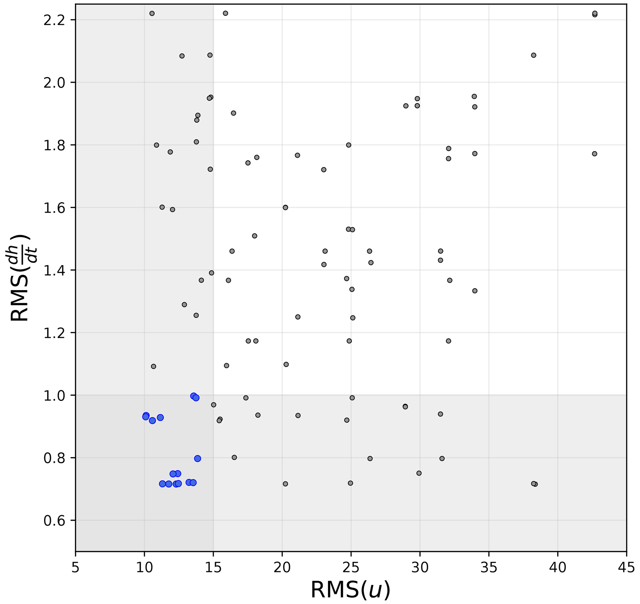
Figure A1Ensemble of inversions (100 members, grey and blue points) in space. The vertical and horizontal grey boxes represent the sub-spaces RMS(u)<15 m a−1 and m a−1. The intersection of the two boxes represents the optimal sub-space (Ω15), which contains 15 members (blue points).
A2 On the use of a diagnostic ice flow model
Klein et al. (2020) reported that the initial state obtained after inversion is not perfectly stable because of remaining uncertainties in other ice sheet parameters (see also e.g. Seroussi et al., 2011), which leads to locally large and unphysical ice thickness rates of change when running transient simulations (e.g. Brondex et al., 2019; Gillet-Chaulet et al., 2012; Klein et al., 2020). This problem is usually overcome by running a relaxation experiment, where the model is allowed to evolve under a constant forcing until a more stable state is reached and before applying the desired perturbation (e.g. Brondex et al., 2019; Gillet-Chaulet et al., 2012). However, this procedure sometimes incurs a significant cost in terms of the differences between observations and the modelled ice thickness and velocities. Although our initial states are similar to those in Klein et al. (2020), our experiment differs by the nature of the perturbation we apply. The basal melting investigated by Klein et al. (2020) directly affects the ice thickness, leading to a modification of the ice flow. The SSH deviations used here do not directly modify the ice thickness but rather modify the driving stress and grounding line position, which leads to a modification of the ice flow, eventually leading to a dynamical change in ice thickness. These changes in ice thickness are fairly small and can be neglected compared with changes in driving stress and grounding line position. Therefore, our model does not actually vary in time; instead, we apply the monthly averaged ΔSSH as a perturbation to the shallow-shelf model and calculate the difference in the velocity field between the perturbed model and the reference model. Monthly velocity change can therefore be determined and compared with the GNSS velocity variations.
B1 Theory and equations
The grounding line migration under tidal variation is usually treated as a purely elastic and hydrostatic problem (Tsai and Gudmundsson, 2015). In this context, at the grounding line, the ice is lifted due to floatation, and the upward buoyancy force in the water column is compensated by the downward gravitational force in the ice column:
where zsl is the sea level, zb is the ice bed elevation, ρi is the ice density, and ρw is the water density.
Adapting Tsai and Gudmundson (2015), upstream from the grounding line, we can approximate the bed elevation at the point of migration by
with β being the bed slope (equal to the ice base slope if located upstream the grounding line) and ΔL the grounding line migration we try to estimate. Similarly, the ice thickness upstream the grounding line can be estimated as
with α being the surface slope. From there, we can rewrite
and estimate
For the downstream migration, our assumption leads to a reduction of the ice base slope by a factor and therefore a potential grounding line migration:
Combining Eqs. (B5) and (B6), we obtain the following parameterisation:
where ΔS± is the SSH perturbation in the grounding zone and
This parameterisation assumes the surface and bed slope to be constant in the grounding zone, while average surface and bed slopes are potentially different immediately upstream versus immediately downstream of the grounding line. However, these differences are unlikely to ever be ∼10 times different. This is especially true for small migrations such as the ones of our hydrostatic model ΔLB2, i.e. about a few tens of metres except in some areas of the Siple Coast and some Transantarctic Mountain glaciers (Fig. S8a); these migration distances are less than our model resolution and below the scales at which we expect large surface and bed slope variations. We also note that the effect of the larger ΔLB2 over the Siple Coast (Fig. S8a) is mitigated by a relatively low basal shear stress, limiting the effect of the migration on the ice flow (Fig. S8b).
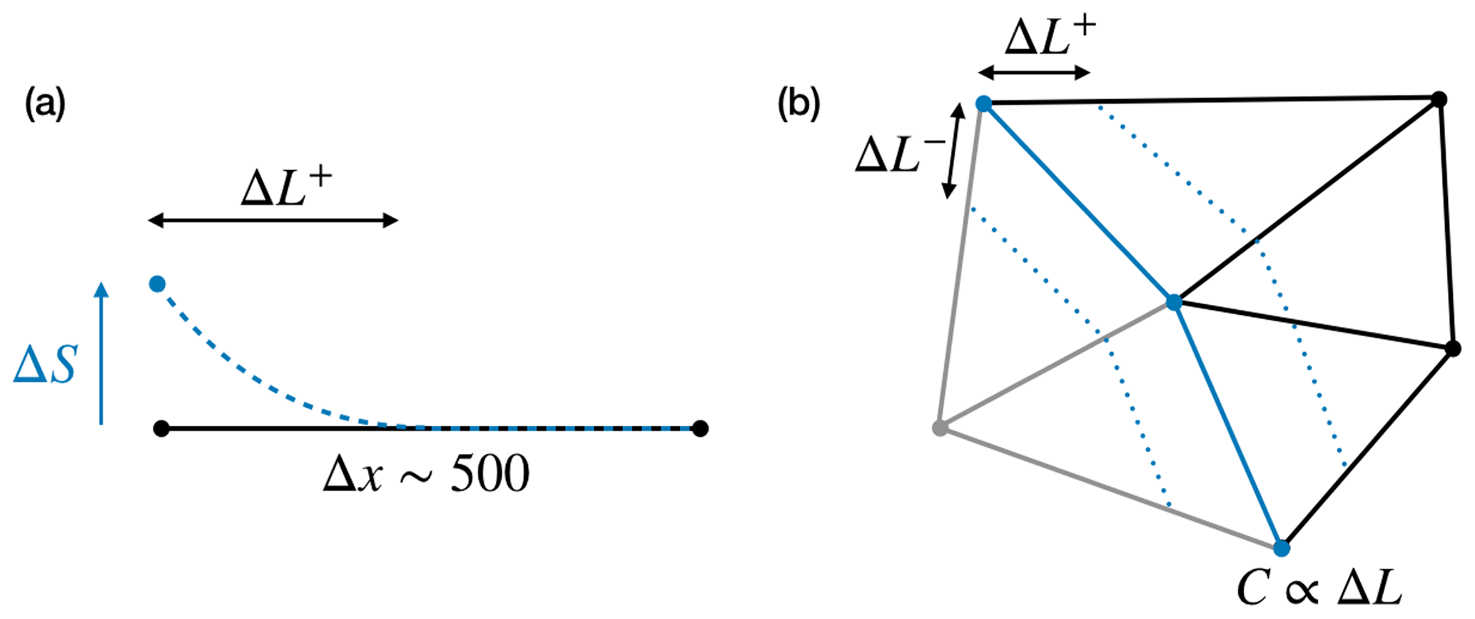
Figure B1Schematic representation of the grounding line migration with sea surface height change (ΔS). (a) Flowline view with Δx being the element edge size at the grounding line and ΔL+ the upstream migration of the grounding line. (b) Two-dimensional plan view of the virtual migration (dotted blue line) of the grounding line (blue line) to an upstream (ΔL+) and downstream location (ΔL−); the evolution of the friction coefficient (C) is proportional to ΔL±. Black and grey elements are initially grounded and floating.
B2 Parameterisations applied to the ice sheet model
The three parameterisations used in our study and presented in Sect. 2.3.2 are further detailed here:
-
ΔLB2. We calculated ΔLB2 by applying γB2 values corresponding to Bedmap2 bed slopes (e.g. and surface slopes (e.g. on the ice shelf and at the grounding line and when averaged over the entire basin) in Eq. (B8), where γ controls the length of the grounding line migration for a given ΔSSH. In the hydrostatic case, γB2 is calculated as a function of α and β.
-
ΔLC. Following Rosier and Gudmundsson (2020), we calculated ΔLC by applying constants for positive and negative bed slopes in Eq. (B8).
-
ΔLB2L. We calculated ΔLB2L by applying a coefficient , with γB2L capped to to limit extremely large grounding line migration in regions with very small γB2L values. This scaling factor was chosen so that the mean migration distance around the RIS perimeter was similar to ΔLC.
B3 Subgrid-scale parameterisation
For cm (roughly the maximal modelled ΔSSH for RIS), , and , Eqs. (B7) and (B8) lead to a m upstream and m downstream migration of the grounding line. These values are much smaller than the Δx∼500 m spacing of our model grid nodes in the vicinity of the grounding line.
We overcome this problem by parameterising the grounding line migration as a variation of the friction coefficient at the grounding line (Fig. B1). We define the initial basal shear force (“i” subscript – before migration) over the element edges surrounding grounding line nodes as
with τi=Ci|ui|m, where Ci is the reference friction coefficient, and ui is the velocity on an element edge; we can write the shear force over a fraction Δx−ΔL of the last grounded element edge as
Equation (B4) can also be written as a function of a final shear stress (“f” subscript – after migration) integrated over the entire element:
with τf=Cf|uf|m where Cf is the friction coefficient at the grounded line node after migration of the grounding line.
Assuming , we can rewrite
with Cf<Ci for ΔL>0 and Cf>Ci for ΔL<0.
The Elmer/Ice code is publicly available through GitHub (https://github.com/ElmerCSC/elmerfem (last access: March 2023) and https://doi.org/10.5281/zenodo.7892181; Ruokolainen et al., 2023; Gagliardini et al., 2013). All the simulations were performed with version 8.3 (rev: b213b0c8) of Elmer/Ice. All Python 3 scripts used for simulations and post-treatment as well as model output are available upon request from the authors. The data used are listed in the references. GNSS data for GZ19 can be accessed at the UNAVCO data centre (https://doi.org/10.7283/T53R0RPD; Siegfried et al., 2014b). The IBE data were generated using Copernicus Climate Change Service Information (2020).
The supplement related to this article is available online at: https://doi.org/10.5194/tc-17-2585-2023-supplement.
CM, LP, and HAF designed the study. CM conducted the simulations. CM and LP conducted the data analyses. EK and PDB provided the DRRIS data and insights into the interpretation of the data. All co-authors contributed to the writing of the paper.
The contact author has declared that none of the authors has any competing interests.
Publisher's note: Copernicus Publications remains neutral with regard to jurisdictional claims in published maps and institutional affiliations.
The authors thank the editor, Jan De Rydt, as well as the two anonymous reviewers for their insightful and helpful comments. This research uses the data services provided by the UNAVCO facility with support from the National Science Foundation (NSF) and the National Aeronautics and Space Administration (NASA) under NSF cooperative agreement EAR-0735156 (GZ19) and EAR-1724794 (BATG). The authors thank Richard Ray and colleagues for providing LORG GNSS data and Scott Springer, Mike Dinniman, Kaitlin Naughten, Ole Ritcher, Pierre Mathiot, and Nicolas Jourdain for providing SSH fields from their ocean models. The authors also thank Till Wagner, Pierre Mathiot, and Nicolas Jourdain for their valuable comments and discussions on this paper.
Cyrille Mosbeux, Laurie Padman, and Helen A. Fricker were supported by NASA (grant nos. 80NSSC20K0977, NNX17AG63G, and NNX17AI03G) and by the NSF (grant nos. 1443677 and 1443498). Laurie Padman was also supported by the NSF (grant no. 1744789). Peter D. Bromirski was supported by the NSF (grant nos. PLR-1246151 and OPP-1744856). The modelling in this work used the Extreme Science and Engineering Discovery Environment (XSEDE), which is supported by the NSF (grant no. TG-DPP190003).
This paper was edited by Jan De Rydt and reviewed by two anonymous referees.
Adusumilli, S., Fricker, H. A., Medley, B., Padman, L., and Siegfried, M. R.: Interannual variations in meltwater input to the Southern Ocean from Antarctic ice shelves, Nat. Geosci., 13, 616–620, https://doi.org/10.1038/s41561-020-0616-z, 2020.
Allison, I., Bindoff, N. L., Bindschadler, R. A., Cox, P. M., de Noblet, N., England, M. H., Francis, J. E., Gruber, N., Haywood, A. M., Karoly, D. J., Kaser, G., Le Quere, C., Lenton, T. M., Mann, M. E., McNeil, B. I., Pitman, A. J., Rahmstorf, S., Rignot, E., Schellnhuber, H. J., Schneider, S. H., Sherwood, S. C., Somerville, R. C. J., Steffen, K., Steig, E. J., Visbeck, M., and Weaver, A. J.: The Copenhagen Diagnosis: Updating the World on the Latest Climate Science, Elsevier, Oxford, UK, 2011.
Armitage, T. W. K., Kwok, R., Thompson, A. F., and Cunningham, G.: Dynamic Topography and Sea Level Anomalies of the Southern Ocean: Variability and Teleconnections, J. Geophys. Res.-Oceans, 123, 613–630, https://doi.org/10.1002/2017JC013534, 2018.
Arthern, R. J. and Wingham, D. J.: The Natural Fluctuations of Firn Densification and Their Effect on the Geodetic Determination of Ice Sheet Mass Balance, Clim. Change, 40, 605–624, https://doi.org/10.1023/A:1005320713306, 1998.
Begeman, C. B., Tulaczyk, S., Padman, L., King, M., Siegfried, M. R., Hodson, T. O., and Fricker, H. A.: Tidal Pressurization of the Ocean Cavity Near an Antarctic Ice Shelf Grounding Line, J. Geophys. Res.-Oceans, 125, e2019JC015562, https://doi.org/10.1029/2019JC015562, 2020.
Blewitt, G., Hammond, W. C., and Kreemer, C.:Harnessing the GPS data explosion for interdisciplinary science, EOS, 99, https://doi.org/10.1029/2018EO104623, 2018.
Bromirski, P. D., Chen, Z., Stephen, R. A., Gerstoft, P., Arcas, D., Diez, A., Aster, R. C., Wiens, D. A., and Nyblade, A.: Tsunami and infragravity waves impacting Antarctic ice shelves, J. Geophys. Res.-Oceans, 122, 5786–5801, https://doi.org/10.1002/2017JC012913, 2017.
Brondex, J., Gillet-Chaulet, F., and Gagliardini, O.: Sensitivity of centennial mass loss projections of the Amundsen basin to the friction law, The Cryosphere, 13, 177–195, https://doi.org/10.5194/tc-13-177-2019, 2019.
Brunt, K. M. and MacAyeal, D. R.: Tidal modulation of ice-shelf flow: a viscous model of the Ross Ice Shelf, J. Glaciol., 60, 500–508, https://doi.org/10.3189/2014JoG13J203, 2014.
Brunt, K. M., Fricker, H. A., and Padman, L.: Analysis of ice plains of the Filchnerâ – Ronne Ice Shelf, Antarctica, using ICESat laser altimetry, J. Glaciol., 57, 965–975, https://doi.org/10.3189/002214311798043753, 2011.
Budd, W. F., Keage, P. L., and Blundy, N. A.: Empirical Studies of Ice Sliding, J. Glaciol., 23, 157–170, https://doi.org/10.3189/S0022143000029804, 1979.
Cook, A. J. and Vaughan, D. G.: Overview of areal changes of the ice shelves on the Antarctic Peninsula over the past 50 years, The Cryosphere, 4, 77–98, https://doi.org/10.5194/tc-4-77-2010, 2010.
Cuffey, K. M. and Paterson, W. S. B.: The Physics of Glaciers, Academic Press, New York, 2010.
Das, I., Padman, L., Bell, R. E., Fricker, H. A., Tinto, K. J., Hulbe, C. L., Siddoway, C. S., Dhakal, T., Frearson, N. P., Mosbeux, C., Cordero, S. I., and Siegfried, M. R.: Multidecadal Basal Melt Rates and Structure of the Ross Ice Shelf, Antarctica, Using Airborne Ice Penetrating Radar, J. Geophys. Res.-Earth Surf., 125, e2019JF005241, https://doi.org/10.1029/2019JF005241, 2020.
Davis, C. H. and Moore, R. K.: A combined surface-and volume-scattering model for ice-sheet radar altimetry, J. Glaciol., 39, 675–686, https://doi.org/10.3189/S0022143000016579, 1993.
Dee, D. P., Uppala, S. M., Simmons, A. J., Berrisford, P., Poli, P., Kobayashi, S., Andrae, U., Balmaseda, M. A., Balsamo, G., Bauer, P., Bechtold, P., Beljaars, A. C. M., van de Berg, L., Bidlot, J., Bormann, N., Delsol, C., Dragani, R., Fuentes, M., Geer, A. J., Haimberger, L., Healy, S. B., Hersbach, H., Hólm, E. V., Isaksen, L., Kållberg, P., Köhler, M., Matricardi, M., McNally, A. P., Monge-Sanz, B. M., Morcrette, J.-J., Park, B.-K., Peubey, C., de Rosnay, P., Tavolato, C., Thépaut, J.-N., and Vitart, F.: The ERA-Interim reanalysis: configuration and performance of the data assimilation system, Q. J. Roy. Meteor. Soc., 137, 553–597, https://doi.org/10.1002/qj.828, 2011.
Depoorter, M. A., Bamber, J. L., Griggs, J. A., Lenaerts, J. T. M., Ligtenberg, S. R. M., van den Broeke, M. R., and Moholdt, G.: Calving fluxes and basal melt rates of Antarctic ice shelves, Nature, 502, 89–92, https://doi.org/10.1038/nature12567, 2013.
Dinniman, M. S., St-Laurent, P., Arrigo, K. R., Hofmann, E. E., and Dijken, G. L. v.: Analysis of Iron Sources in Antarctic Continental Shelf Waters, J. Geophys. Res.-Oceans, 125, e2019JC015736, https://doi.org/10.1029/2019JC015736, 2020.
Dutrieux, P., De Rydt, J., Jenkins, A., Holland, P. R., Ha, H. K., Lee, S. H., Steig, E. J., Ding, Q., Abrahamsen, E. P., and Schröder, M.: Strong Sensitivity of Pine Island Ice-Shelf Melting to Climatic Variability, Science, 343, 174–178, https://doi.org/10.1126/science.1244341, 2014.
Fretwell, P., Pritchard, H. D., Vaughan, D. G., Bamber, J. L., Barrand, N. E., Bell, R., Bianchi, C., Bingham, R. G., Blankenship, D. D., Casassa, G., Catania, G., Callens, D., Conway, H., Cook, A. J., Corr, H. F. J., Damaske, D., Damm, V., Ferraccioli, F., Forsberg, R., Fujita, S., Gim, Y., Gogineni, P., Griggs, J. A., Hindmarsh, R. C. A., Holmlund, P., Holt, J. W., Jacobel, R. W., Jenkins, A., Jokat, W., Jordan, T., King, E. C., Kohler, J., Krabill, W., Riger-Kusk, M., Langley, K. A., Leitchenkov, G., Leuschen, C., Luyendyk, B. P., Matsuoka, K., Mouginot, J., Nitsche, F. O., Nogi, Y., Nost, O. A., Popov, S. V., Rignot, E., Rippin, D. M., Rivera, A., Roberts, J., Ross, N., Siegert, M. J., Smith, A. M., Steinhage, D., Studinger, M., Sun, B., Tinto, B. K., Welch, B. C., Wilson, D., Young, D. A., Xiangbin, C., and Zirizzotti, A.: Bedmap2: improved ice bed, surface and thickness datasets for Antarctica, The Cryosphere, 7, 375–393, https://doi.org/10.5194/tc-7-375-2013, 2013.
Fürst, J. J., Durand, G., Gillet-Chaulet, F., Merino, N., Tavard, L., Mouginot, J., Gourmelen, N., and Gagliardini, O.: Assimilation of Antarctic velocity observations provides evidence for uncharted pinning points, The Cryosphere, 9, 1427–1443, https://doi.org/10.5194/tc-9-1427-2015, 2015.
Fürst, J. J., Durand, G., Gillet-Chaulet, F., Tavard, L., Rankl, M., Braun, M., and Gagliardini, O.: The safety band of Antarctic ice shelves, Nat. Clim. Change, 6, 479–482, https://doi.org/10.1038/nclimate2912, 2016.
Gagliardini, O., Zwinger, T., Gillet-Chaulet, F., Durand, G., Favier, L., de Fleurian, B., Greve, R., Malinen, M., Martín, C., Råback, P., Ruokolainen, J., Sacchettini, M., Schäfer, M., Seddik, H., and Thies, J.: Capabilities and performance of Elmer/Ice, a new-generation ice sheet model, Geosci. Model Dev., 6, 1299–1318, https://doi.org/10.5194/gmd-6-1299-2013, 2013.
Geng, J., Shi, C., Ge, M., Dodson, A. H., Lou, Y., Zhao, Q., and Liu, J.: Improving the estimation of fractional-cycle biases for ambiguity resolution in precise point positioning, J. Geod., 86, 579–589, https://doi.org/10.1007/s00190-011-0537-0, 2012.
Geng, J., Chen, X., Pan, Y., Mao, S., Li, C., Zhou, J., and Zhang, K.: PRIDE PPPAR: an open-source software for GPS PPP ambiguity resolution, GPS Solut., 23, 91, https://doi.org/10.1007/s10291-019-0888-1, 2019.
Gillet-Chaulet, F., Gagliardini, O., Seddik, H., Nodet, M., Durand, G., Ritz, C., Zwinger, T., Greve, R., and Vaughan, D. G.: Greenland ice sheet contribution to sea-level rise from a new-generation ice-sheet model, The Cryosphere, 6, 1561–1576, https://doi.org/10.5194/tc-6-1561-2012, 2012.
Gillet‐Chaulet, F., Durand, G., Gagliardini, O., Mosbeux, C., Mouginot, J., Rémy, F., and Ritz, C.: Assimilation of surface velocities acquired between 1996 and 2010 to constrain the form of the basal friction law under Pine Island Glacier, Geophys. Res. Lett., 43, 10311–10321, https://doi.org/10.1002/2016GL069937, 2016.
Glen, J. W.: The Creep of Polycrystalline Ice, P. Roy. Soc. Lond. A, 228, 519–538, https://doi.org/10.1098/rspa.1955.0066, 1958.
Goring, D. G. and Pyne, A.: Observations of sea-level variability in Ross Sea, Antarctica, New Zeal. J. Mar. Fresh., 37, 241–249, https://doi.org/10.1080/00288330.2003.9517162, 2003.
Greatbatch, R. J.: A note on the representation of steric sea level in models that conserve volume rather than mass, J. Geophys. Res.-Oceans, 99, 12767–12771, https://doi.org/10.1029/94JC00847, 1994.
Greene, C. A., Young, D. A., Gwyther, D. E., Galton-Fenzi, B. K., and Blankenship, D. D.: Seasonal dynamics of Totten Ice Shelf controlled by sea ice buttressing, The Cryosphere, 12, 2869–2882, https://doi.org/10.5194/tc-12-2869-2018, 2018.
Greene, C. A., Gardner, A. S., and Andrews, L. C.: Detecting seasonal ice dynamics in satellite images, The Cryosphere, 14, 4365–4378, https://doi.org/10.5194/tc-14-4365-2020, 2020.
Gudmundsson, G. H.: Tides and the flow of Rutford Ice Stream, West Antarctica, J. Geophys. Res.-Earth Surf., 112, F04007, https://doi.org/10.1029/2006JF000731, 2007.
Gudmundsson, G. H.: Ice-shelf buttressing and the stability of marine ice sheets, The Cryosphere, 7, 647–655, https://doi.org/10.5194/tc-7-647-2013, 2013.
Gudmundsson, G. H., Paolo, F. S., Adusumilli, S., and Fricker, H. A.: Instantaneous Antarctic ice sheet mass loss driven by thinning ice shelves, Geophys. Res. Lett., 46, 13903–13909, https://doi.org/10.1029/2019GL085027, 2019.
Hersbach, H., Bell, B., Berrisford, P., Hirahara, S., Horányi, A., Muñoz-Sabater, J., Nicolas, J., Peubey, C., Radu, R., Schepers, D., Simmons, A., Soci, C., Abdalla, S., Abellan, X., Balsamo, G., Bechtold, P., Biavati, G., Bidlot, J., Bonavita, M., Chiara, G. D., Dahlgren, P., Dee, D., Diamantakis, M., Dragani, R., Flemming, J., Forbes, R., Fuentes, M., Geer, A., Haimberger, L., Healy, S., Hogan, R. J., Hólm, E., Janisková, M., Keeley, S., Laloyaux, P., Lopez, P., Lupu, C., Radnoti, G., Rosnay, P. de, Rozum, I., Vamborg, F., Villaume, S., and Thépaut, J.-N.: The ERA5 global reanalysis, Q. J. Roy. Meteor. Soc., 146, 1999–2049, https://doi.org/10.1002/qj.3803, 2020.
Jenkins, A., Shoosmith, D., Dutrieux, P., Jacobs, S., Kim, T. W., Lee, S. H., Ha, H. K., and Stammerjohn, S.: West Antarctic Ice Sheet retreat in the Amundsen Sea driven by decadal oceanic variability, Nat. Geosci., 11, 733–738, https://doi.org/10.1038/s41561-018-0207-4, 2018.
Joughin, I., Bindschadler, R. A., King, M. A., Voigt, D., Alley, R. B., Anandakrishnan, S., Horgan, H., Peters, L., Winberry, P., Das, S. B., and Catania, G.: Continued deceleration of Whillans Ice Stream, West Antarctica, Geophys. Res. Lett., 32, L22501, https://doi.org/10.1029/2005GL024319, 2005.
Joughin, I., Smith, B. E., and Medley, B.: Marine Ice Sheet Collapse Potentially Under Way for the Thwaites Glacier Basin, West Antarctica, Science, 344, 735–738, https://doi.org/10.1126/science.1249055, 2014.
Joughin, I., Smith, B. E., and Schoof, C. G.: Regularized Coulomb Friction Laws for Ice Sheet Sliding: Application to Pine Island Glacier, Antarctica, Geophys. Res. Lett., 46, 4764–4771, https://doi.org/10.1029/2019GL082526, 2019.
Kazmierczak, E., Sun, S., Coulon, V., and Pattyn, F.: Subglacial hydrology modulates basal sliding response of the Antarctic ice sheet to climate forcing, The Cryosphere, 16, 4537–4552, https://doi.org/10.5194/tc-16-4537-2022, 2022.
Klein, E., Mosbeux, C., Bromirski, P. D., Padman, L., Bock, Y., Springer, S. R., and Fricker, H. A.: Annual cycle in flow of Ross Ice Shelf, Antarctica: contribution of variable basal melting, J. Glaciol., 66, 861–875, https://doi.org/10.1017/jog.2020.61, 2020.
Larour, E., Seroussi, H., Adhikari, S., Ivins, E., Caron, L., Morlighem, M., and Schlegel, N.: Slowdown in Antarctic mass loss from solid Earth and sea-level feedbacks, Science, 364, eaav7908, https://doi.org/10.1126/science.aav7908, 2019.
MacAyeal, D. R.: Large-scale ice flow over a viscous basal sediment: Theory and application to ice stream B, Antarctica, J. Geophys. Res.-Sol. Ea., 94, 4071–4087, https://doi.org/10.1029/JB094iB04p04071, 1989.
Makinson, K., King, M. A., Nicholls, K. W., and Gudmundsson, G. H.: Diurnal and semidiurnal tide-induced lateral movement of Ronne Ice Shelf, Antarctica, Geophys. Res. Lett., 39, L10501, https://doi.org/10.1029/2012GL051636, 2012.
Mathiot, P., Jenkins, A., Harris, C., and Madec, G.: Explicit representation and parametrised impacts of under ice shelf seas in the z* coordinate ocean model NEMO 3.6, Geosci. Model Dev., 10, 2849–2874, https://doi.org/10.5194/gmd-10-2849-2017, 2017.
Mellor, G. L. and Ezer, T.: Sea level variations induced by heating and cooling: An evaluation of the Boussinesq approximation in ocean models, J. Geophys. Res.-Oceans, 100, 20565–20577, https://doi.org/10.1029/95JC02442, 1995.
Morland, L. W.: Dynamics of the West Antarctic Ice Sheet: Unconfined Ice-Shelf Flow, Glaciology and Quaternary Geology, edited by: Van der Veen, C. J. and Oerlemans, J., Springer Netherlands, https://doi.org/10.1007/978-94-009-3745-1, 1987.
Mosbeux, C., Gillet-Chaulet, F., and Gagliardini, O.: Comparison of adjoint and nudging methods to initialise ice sheet model basal conditions, Geosci. Model Dev., 9, 2549–2562, https://doi.org/10.5194/gmd-9-2549-2016, 2016.
Naughten, K. A., Meissner, K. J., Galton-Fenzi, B. K., England, M. H., Timmermann, R., Hellmer, H. H., Hattermann, T., and Debernard, J. B.: Intercomparison of Antarctic ice-shelf, ocean, and sea-ice interactions simulated by MetROMS-iceshelf and FESOM 1.4, Geosci. Model Dev., 11, 1257–1292, https://doi.org/10.5194/gmd-11-1257-2018, 2018.
Padman, L., Erofeeva, S., and Joughin, I.: Tides of the Ross Sea and Ross Ice Shelf cavity, Antarct. Sci., 15, 31–40, https://doi.org/10.1017/S0954102003001032, 2003.
Paolo, F. S., Fricker, H. A., and Padman, L.: Volume loss from Antarctic ice shelves is accelerating, Science, 348, 327–331, https://doi.org/10.1126/science.aaa0940, 2015.
Paolo, F. S., Padman, L., Fricker, H. A., Adusumilli, S., Howard, S., and Siegfried, M. R.: Response of Pacific-sector Antarctic ice shelves to the El Nino/Southern Oscillation, Nat. Geosci., 1, 121–126, https://doi.org/10.1038/s41561-017-0033-0, 2018.
Parish, T. R. and Bromwich, D. H.: On the forcing of seasonal changes in surface pressure over Antarctica, J. Geophys. Res.-Atmos., 102, 13785–13792, https://doi.org/10.1029/96JD02959, 1997.
Pattyn, F., Perichon, L., Durand, G., Favier, L., Gagliardini, O., Hindmarsh, R. C. A., Zwinger, T., Albrecht, T., Cornford, S., Docquier, D., Fürst, J. J., Goldberg, D., Gudmundsson, G. H., Humbert, A., Hütten, M., Huybrechts, P., Jouvet, G., Kleiner, T., Larour, E., Martin, D., Morlighem, M., Payne, A. J., Pollard, D., Rückamp, M., Rybak, O., Seroussi, H., Thoma, M., and Wilkens, N.: Grounding-line migration in plan-view marine ice-sheet models: results of the ice2sea MISMIP3d intercomparison, J. Glaciol., 59, 410–422, https://doi.org/10.3189/2013JoG12J129, 2013.
Ray, R., Larson, K., and Haines, B.: New determinations of tides on the north-western Ross Ice Shelf, Antarct. Sci., 33, 89–102, https://doi.org/10.1017/S0954102020000498, 2021.
Reese, R., Winkelmann, R., and Gudmundsson, G. H.: Grounding-line flux formula applied as a flux condition in numerical simulations fails for buttressed Antarctic ice streams, The Cryosphere, 12, 3229–3242, https://doi.org/10.5194/tc-12-3229-2018, 2018.
Richter, O., Gwyther, D. E., Galton-Fenzi, B. K., and Naughten, K. A.: The Whole Antarctic Ocean Model (WAOM v1.0): development and evaluation, Geosci. Model Dev., 15, 617–647, https://doi.org/10.5194/gmd-15-617-2022, 2022.
Ridley, J. K. and Partingon, K. C.: A model of satellite radar altimeter return from ice sheets, Int. J. Remote Sens., 9, 601–624, https://doi.org/10.1080/01431168808954881, 1988.
Rignot, E., Mouginot, J., and Scheuchl, B.: Ice Flow of the Antarctic Ice Sheet, Science, 333, 1427–1430, https://doi.org/10.1126/science.1208336, 2011.
Rignot, E., Mouginot, J., and Scheuchl, B.: MEaSUREs InSAR-based Antarctica Ice Velocity map, Version 2. NASA National Snow and Ice Data Center Distributed Active Archive Center, Boulder, Colorado, USA [data set], https://doi.org/10.5067/D7GK8F5J8M8R, 2017.
Robel, A. A., Wilson, E., and Seroussi, H.: Layered seawater intrusion and melt under grounded ice, The Cryosphere, 16, 451–469, https://doi.org/10.5194/tc-16-451-2022, 2022.
Rosier, S. H. R. and Gudmundsson, G. H.: Exploring mechanisms responsible for tidal modulation in flow of the Filchner–Ronne Ice Shelf, The Cryosphere, 14, 17–37, https://doi.org/10.5194/tc-14-17-2020, 2020.
Rosier, S. H. R., Gudmundsson, G. H., and Green, J. A. M.: Insights into ice stream dynamics through modelling their response to tidal forcing, The Cryosphere, 8, 1763–1775, https://doi.org/10.5194/tc-8-1763-2014, 2014.
Ruokolainen, J., Malinen, M., Råback, P., Zwinger, T., Takala, E., Kataja, J., Gillet-Chaulet, F., Ilvonen, S., Gladstone, R., Byckling, M., Chekki, M., Gong, C., Ponomarev, P., van Dongen, E., Robertsen, F., Wheel, I., Cook, S., t7saeki, luzpaz, and Rich_B: ElmerCSC/elmerfem, Zenodo [code], https://doi.org/10.5281/zenodo.7892181, 2023.
Rye, C. D., Naveira Garabato, A. C., Holland, P. R., Meredith, M. P., George Nurser, A. J., Hughes, C., Coward, A. C., and Webb, D. J.: Rapid sea-level rise along the Antarctic margins in response to increased glacial discharge, Nat. Geosci, 7, 732–735, 2014.
Sayag, R. and Worster, M. G.: Elastic response of a grounded ice sheet coupled to a floating ice shelf, Phys. Rev. E, 84, 036111, https://doi.org/10.1103/PhysRevE.84.036111, 2011.
Sayag, R. and Worster, M. G.: Elastic dynamics and tidal migration of grounding lines modify subglacial lubrication and melting, Geophys. Res. Lett., 40, 5877–5881, https://doi.org/10.1002/2013GL057942, 2013.
Scambos, T. A., Bohlander, J. A., Shuman, C. A., and Skvarca, P.: Glacier acceleration and thinning after ice shelf collapse in the Larsen B embayment, Antarctica, Geophys. Res. Lett., 31, L18402, https://doi.org/10.1029/2004GL020670, 2004.
Schoof, C.: The effect of cavitation on glacier sliding, P. Roy. Soc. Lond. A, 461, 609–627, https://doi.org/10.1098/rspa.2004.1350, 2005.
Seroussi, H., Morlighem, M., Rignot, E., Larour, E., Aubry, D., Ben Dhia, H., and Kristensen, S. S.: Ice flux divergence anomalies on 79north Glacier, Greenland, Geophys. Res. Lett., 38, L09501, https://doi.org/10.1029/2011GL047338, 2011.
Siegfried, M. R., Fricker, H. A., Roberts, M., Scambos, T. A., and Tulaczyk, S.: A decade of West Antarctic subglacial lake interactions from combined ICESat and CryoSat-2 altimetry, Geophys. Res. Lett., 41, 891–898, https://doi.org/10.1002/2013GL058616, 2014a.
Siegfried, M. R., Fricker, H. A., and Tulaczyk, S.: Antarctica PI Continuous – GZ19-WIS_GroundingZone_19 P.S., The GAGE Facility operated by EarthScope Consortium, GPS/GNSS Observations [data set], https://doi.org/10.7283/T53R0RPD, 2014b.
Smith, B., Fricker, H. A., Gardner, A. S., Medley, B., Nilsson, J., Paolo, F. S., Holschuh, N., Adusumilli, S., Brunt, K., Csatho, B., Harbeck, K., Markus, T., Neumann, T., Siegfried, M. R., and Zwally, H. J.: Pervasive ice sheet mass loss reflects competing ocean and atmosphere processes, Science, 368, 1239–1242, https://doi.org/10.1126/science.aaz5845, 2020.
Stearns, L. A., Smith, B. E., and Hamilton, G. S.: Increased flow speed on a large East Antarctic outlet glacier caused by subglacial floods, Nat. Geosci., 1, 827–831, https://doi.org/10.1038/ngeo356, 2008.
Stewart, C. L., Christoffersen, P., Nicholls, K. W., Williams, M. J. M., and Dowdeswell, J. A.: Basal melting of Ross Ice Shelf from solar heat absorption in an ice-front polynya, Nat. Geosci., 12, 435–440, https://doi.org/10.1038/s41561-019-0356-0, 2019.
Thomas, R., Scheuchl, B., Frederick, E., Harpold, R., Martin, C., and Rignot, E.: Continued slowing of the Ross Ice Shelf and thickening of West Antarctic ice streams, J. Glaciol., 59, 838–844, https://doi.org/10.3189/2013JoG12J122, 2013.
Thomas, R. H.: Ice Shelves: A Review, J. Glaciol., 24, 273–286, https://doi.org/10.3189/S0022143000014799, 1979.
Tinto, K. J., Padman, L., Siddoway, C. S., Springer, S. R., Fricker, H. A., Das, I., Tontini, F. C., Porter, D. F., Frearson, N. P., Howard, S. L., Siegfried, M. R., Mosbeux, C., Becker, M. K., Bertinato, C., Boghosian, A., Brady, N., Burton, B. L., Chu, W., Cordero, S. I., Dhakal, T., Dong, L., Gustafson, C. D., Keeshin, S., Locke, C., Lockett, A., O'Brien, G., Spergel, J. J., Starke, S. E., Tankersley, M., Wearing, M. G., and Bell, R. E.: Ross Ice Shelf response to climate driven by the tectonic imprint on seafloor bathymetry, Nat. Geosci., 12, 441–449, https://doi.org/10.1038/s41561-019-0370-2, 2019.
Tsai, V. C., Stewart, A. L., and Thompson, A. F.: Marine ice-sheet profiles and stability under Coulomb basal conditions, J. Glaciol., 61, 205–215, 2015.
Tulaczyk, S., Mikucki, J. A., Siegfried, M. R., Priscu, J. C., Barcheck, C. G., Beem, L. H., Behar, A., Burnett, J., Christner, B. C., Fisher, A. T., Fricker, H. A., Mankoff, K. D., Powell, R. D., Rack, F., Sampson, D., Scherer, R. P., Schwartz, S. Y., and Team, T. W. S.: WISSARD at Subglacial Lake Whillans, West Antarctica: scientific operations and initial observations, Ann. Glaciol., 55, 51–58, https://doi.org/10.3189/2014AoG65A009, 2014.
Urruty, B., Hill, E. A., Reese, R., Garbe, J., Gagliardini, O., Durand, G., Gillet-Chaulet, F., Gudmundsson, G. H., Winkelmann, R., Chekki, M., Chandler, D., and Langebroek, P. M.: The stability of present-day Antarctic grounding lines – Part A: No indication of marine ice sheet instability in the current geometry, The Cryosphere Discuss. [preprint], https://doi.org/10.5194/tc-2022-104, in review, 2022.
Velicogna, I., Sutterley, T. C., and Broeke, M. R. v. d.: Regional acceleration in ice mass loss from Greenland and Antarctica using GRACE time-variable gravity data, Geophys. Res. Lett., 41, 8130–8137, https://doi.org/10.1002/2014GL061052, 2014.
Walker, R. T., Parizek, B. R., Alley, R. B., Anandakrishnan, S., Riverman, K. L., and Christianson, K.: Ice-shelf tidal flexure and subglacial pressure variations, Earth Planet. Sc. Lett., 361, 422–428, https://doi.org/10.1016/j.epsl.2012.11.008, 2013.
Weertman, J.: On the Sliding of Glaciers, J. Glaciol., 3, 33–38, https://doi.org/10.3189/S0022143000024709, 1957.
Winberry, J. P., Anandakrishnan, S., Alley, R. B., Bindschadler, R. A., and King, M. A.: Basal mechanics of ice streams: Insights from the stick-slip motion of Whillans Ice Stream, West Antarctica, J. Geophys. Res.-Earth Surf., 114,F01016, https://doi.org/10.1029/2008JF001035, 2009.
Yano, K.: The Theory of Lie Derivatives and its Applications, Courier Dover Publications, North-Holland, Amsterdam, 1957.
Yuan, X., Qiao, G., and Li, Y.: 57-Year Ice Velocity Dynamics in Byrd Glacier Based on Multisource Remote Sensing Data, IEEE J. Sel. Top. Appl. Earth Obs., 16, 2711–2727, https://doi.org/10.1109/JSTARS.2023.3250759, 2023.
Zumberge, J. F., Heflin, M. B., Jefferson, D. C., Watkins, M. M., and Webb, F. H.: Precise point positioning for the efficient and robust analysis of GPS data from large networks, J. Geophys. Res.-Sol. Ea., 102, 5005–5017, https://doi.org/10.1029/96JB03860, 1997.
Zwally, H. J. and Jun, L.: Seasonal and interannual variations of firn densification and ice-sheet surface elevation at the Greenland summit, J. Glaciol., 48, 199–207, https://doi.org/10.3189/172756502781831403, 2002.
- Abstract
- Introduction
- Data and models
- Results and discussion
- Sources of uncertainty in SSH and ice flow response
- Conclusions
- Appendix A: Inverse and direct ice flow model
- Appendix B: Parameterisation of the grounding line migration
- Code and data availability
- Author contributions
- Competing interests
- Disclaimer
- Acknowledgements
- Financial support
- Review statement
- References
- Supplement