A decade-plus of Antarctic sea ice thickness and volume estimates from CryoSat-2 using a physical model and waveform fitting

We estimate the snow depth and snow freeboard of Antarctic sea ice using a comprehensive retrieval method (referred to as CryoSat-2 Waveform Fitting for Antarctic sea ice, or CS2WFA) consisting of a physical waveform model and a waveform-fitting process that fits modeled waveforms to CryoSat-2 data. These snow depth and snow freeboard estimates are combined with snow, sea ice, and sea water density values to calculate the sea ice thickness and volume over an 11+ year span between 2010 and 2021. We first compare our snow freeboard, snow depth, and sea ice thickness estimates to other altimetry- and ship-based observations and find good agreement overall in both along-track and monthly gridded comparisons. Some discrepancies exist in certain regions and seasons that are theorized to come from both sampling biases and the differing assumptions in the retrieval methods. We then present an 11+ year time series of sea ice thickness and volume both regionally and pan-Antarctic. This time series is used to uncover intra-decadal changes in the ice cover between 2010 and 2021, showing small, competing regional thickness changes of less than 0.5 cm yr⁻¹ in magnitude. Finally, we place these thickness estimates in the context of a longer-term, snow freeboard-derived, laser–radar sea ice thickness time series that began with NASA's Ice, Cloud, and land Elevation Satellite (ICESat) and continues with ICESat-2 and contend that reconciling and validating this longer-term, multi-sensor time series will be important in better understanding changes in the Antarctic sea ice cover.

1 Introduction

Sea ice thickness is an important parameter in Earth's climate system, as it controls fluxes of heat, moisture, and salinity between the ocean and atmosphere (Persson and Vihma, 2016). It also acts as an indicator of climate change and variability (EPA, 2016) due to its intimate relationship with other components of the cryosphere. Knowledge of sea ice thickness has long been important in the polar regions – from early Antarctic explorers navigating in icy waters (Herdman, 1959) to indigenous Arctic communities traveling and hunting on the frozen sea (Nichols et al., 2004) – and continues to be a focus today for maritime navigation and climate studies (Meredith et al., 2019). While measuring thickness in situ is a straightforward process – requiring only a hole and a measuring device – the sheer size of the sea ice pack in both hemispheres and the impracticality of routine work in the polar regions limits the ability to manually measure the thickness of the sea ice cover on the basin scale. Instead, satellite altimeters are typically used.

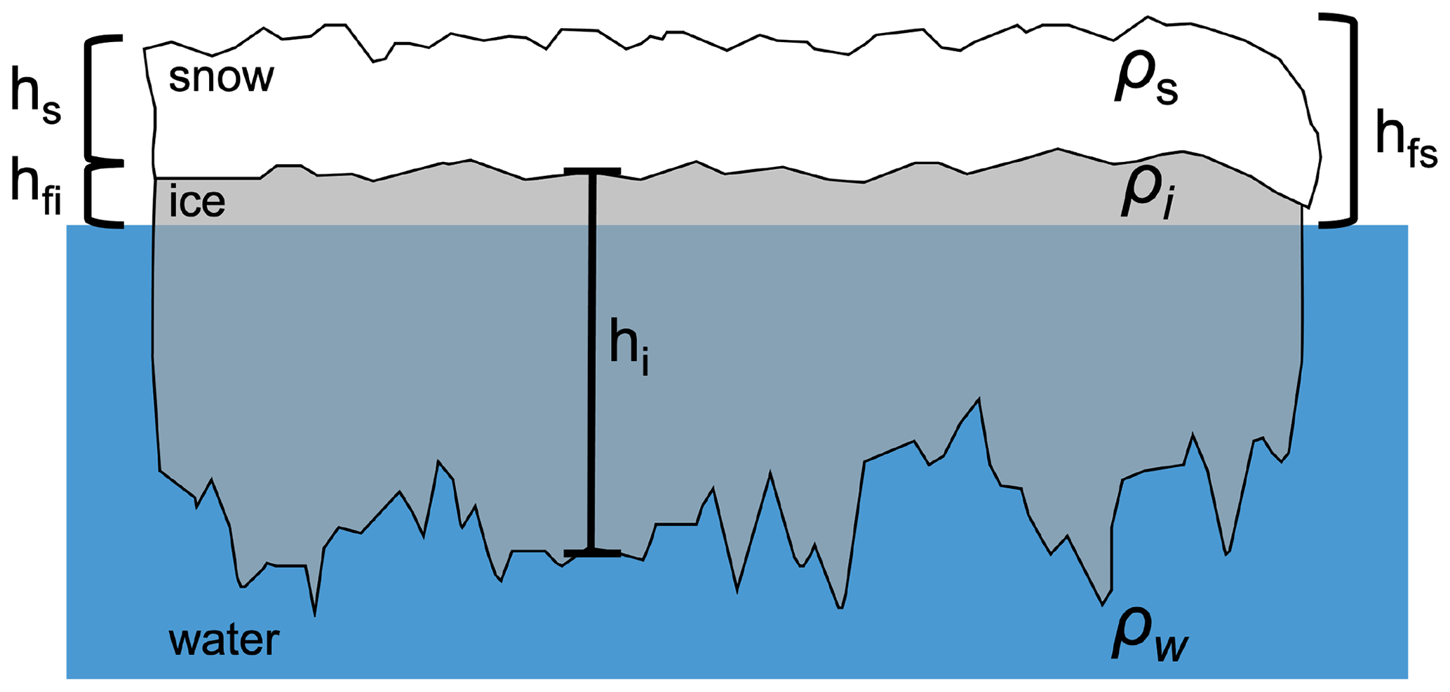
By measuring the height of the sea ice above the local sea surface (i.e., the freeboard) from altimetry, one can apply assumptions of hydrostatic balance to estimate the thickness of the sea ice. Wavelength differences between the two primary types of altimeters – radar and laser – correspond to varying dominant scattering horizons over sea ice and therefore different retrieved freeboards: ice freeboard (assuming the dominant radar scattering comes from the snow–ice interface) and snow freeboard (assuming the dominant laser scattering comes from the air–snow interface), respectively. These two distinct freeboard values require different equations for calculating thickness. If the ice freeboard is known, one can define thickness as

$$\begin{array}{}\text{(1)}& h_{\mathrm{i}-\mathrm{fi}}=\left({\displaystyle \frac{{\mathit{\rho }}_{\mathrm{w}}}{{\mathit{\rho }}_{\mathrm{w}}-{\mathit{\rho }}_{\mathrm{i}}}}\right)h_{\mathrm{fi}}+\left({\displaystyle \frac{{\mathit{\rho }}_{\mathrm{s}}}{{\mathit{\rho }}_{\mathrm{w}}-{\mathit{\rho }}_{\mathrm{i}}}}\right)h_{\mathrm{s}},\end{array}$$

where h_i−fi is the ice thickness computed from the ice freeboard; h_fi is the ice freeboard; h_s is the snow depth; and ρ is the density of seawater (ρ_w), ice (ρ_i), and snow (ρ_s). If the snow freeboard is known, then the equation instead becomes

$$\begin{array}{}\text{(2)}& h_{\mathrm{i}-\mathrm{fs}}=\left({\displaystyle \frac{{\mathit{\rho }}_{\mathrm{w}}}{{\mathit{\rho }}_{\mathrm{w}}-{\mathit{\rho }}_{\mathrm{i}}}}\right)h_{\mathrm{fs}}+\left({\displaystyle \frac{{\mathit{\rho }}_{\mathrm{s}}-{\mathit{\rho }}_{\mathrm{w}}}{{\mathit{\rho }}_{\mathrm{w}}-{\mathit{\rho }}_{\mathrm{i}}}}\right)h_{\mathrm{s}},\end{array}$$

where h_i−fs is the ice thickness computed from the snow freeboard, h_fs is the snow freeboard, and the snow depth and density are as in Eq. (1) (Kurtz and Markus, 2012; Kwok, 2011). It is important to note that in Eq. (2), the second term results in a reduction of the sea ice thickness computed from the first term alone, which is opposite that of Eq. (1) and can play a key role for Antarctic sea ice where snow freeboard may equal (or be less than, in the case of flooding) the snow depth. Equations (1) and (2) clearly show that estimates of freeboard and snow depth are the two necessary measurements for deriving thickness from satellite altimetry.

Figure 1 Schematic showing parameters in Eqs. (1) and (2), including snow depth (h_s), ice freeboard (h_fi), snow freeboard (h_fs), ice thickness (h_i), and the density terms of snow (ρ_s), ice (ρ_i), and seawater (ρ_w).

Over Arctic sea ice, satellite-altimeter-derived freeboard has been estimated since around 2003 using the European Remote Sensing Satellites ERS-1 and ERS-2 (Laxon et al., 2003). The launch of NASA's Ice, Cloud, and land Elevation Satellite (ICESat) in 2003 facilitated snow freeboard measurements between 2003–2008 (Zwally et al., 2002; Kwok et al., 2007; Kurtz et al., 2008; Farrell et al., 2009), while ESA's CryoSat-2 satellite has been used extensively to estimate Arctic sea ice freeboard since its launch in 2010 (Laxon et al., 2013; Kurtz et al., 2014; Ricker et al., 2014; Kwok and Cunningham, 2015; Tilling et al., 2018; Landy et al., 2020). In most of these cases, a regional snow depth climatology built from ground-based measurements collected between 1954–1991 (Warren et al., 1999) is used to convert the freeboard measurements to thickness estimates. More recently, NASA's ICESat-2 satellite has been operating, and studies have combined ICESat-2 freeboards with snow depths from models (e.g., Petty et al., 2018; Liston et al., 2018, 2020) to estimate sea ice thickness (Petty et al., 2020).

While the studies mentioned above were successful in retrieving sea ice thickness from sea ice freeboard estimates over Arctic sea ice, fewer works have done so for Antarctic sea ice. This hemispheric discrepancy is primarily due to two reasons. First, ice freeboard from radar altimetry is difficult to estimate for Antarctic sea ice, since the thicker snow layer on Antarctic sea ice can depress the ice nearer to the ocean surface, leading to flooding, enhanced brine wicking, and other processes that drive complex stratigraphy and complicate returns from Ku-band altimeters (Giovinetto et al., 1992; Maksym and Jeffries, 2000; Willatt et al., 2010). Ground-based studies have shown that assuming a Ku-band radar pulse penetrates to the snow–ice interface is likely incorrect, with dominant returns more likely to originate from within the snow layer or the air–snow interface (Willatt et al., 2010). Second, the snow depth distribution over Antarctic sea ice is not as well-known (Giles et al., 2008). Unlike the Arctic, few ground-based snow depth estimates exist from which thickness can be estimated. Worby et al. (2008) provide seasonal and regional snow depth estimates from ship-based observations; however, these are subject to seasonal and spatial sampling biases due to the location of ship tracks. Other studies have used passive microwave instruments to derive snow depth; however, these measurements contain large pixel-level uncertainties associated with ice type, sensor footprint size, and a lack of validation data (Markus and Cavalieri, 1998; Kern and Ozsoy-Çiçek, 2016; Maksym and Markus, 2008). These barriers mean that using radar altimetry, mainly CryoSat-2, over Antarctic sea ice will increase complexity of and uncertainty in the freeboard retrievals. Also, it means that calculating sea ice thickness will require either assumptions about the snow layer or new basin-wide data sets of snow depth on sea ice.

Some works have attempted to retrieve Antarctic sea ice freeboard from CryoSat-2 (Paul et al., 2018; Schwegmann et al., 2016; Fons and Kurtz, 2019). Schwegmann et al. (2016) estimated radar freeboard, but the lack of snow depth information prevented the correction for wave speed in snow (in order to convert to ice freeboard) and the estimation of thickness. Paul et al. (2018) did correct for wave speed using passive microwave snow depths but did not estimate thickness from the measurements, citing the need for external snow depth data. Fons and Kurtz (2019) estimated snow freeboard from CryoSat-2 using snow scattering information contained in a physical waveform model but also did not estimate thickness, citing a lack of confidence in the snow depth retrievals. Currently, the only Antarctic sea ice thickness products from CryoSat-2 come from the ESA Climate Change Initiative (CCI; Hendricks et al., 2018), which utilized the procedure from Schwegmann et al. (2016) and Paul et al. (2018) in its estimates, and from Garnier et al. (2022), who calibrated Envisat thicknesses with CryoSat-2 to produce a longer time series. However, due to the uncertainties surrounding the radar penetration, snow depth, and the use of power threshold empirical retracking algorithms, these estimates are both assumed to be biased high (Hendricks et al., 2018; Garnier et al., 2022).

Other studies have been able to estimate Antarctic sea ice thickness from laser altimetry – namely ICESat and ICESat-2 – through the use of key snow depth assumptions. One example is Kurtz and Markus (2012), who applied a “zero-ice-freeboard” (ZIF) assumption, which assumes that the snow depth depresses the ice down to the water level everywhere, resulting in a snow depth equal to the snow freeboard and an ice freeboard equal to zero. Under this assumption, Eq. (2) becomes

$$\begin{array}{}\text{(3)}& h_{\mathrm{i}-\mathrm{ZIF}}=\left({\displaystyle \frac{{\mathit{\rho }}_{\mathrm{s}}}{{\mathit{\rho }}_{\mathrm{w}}-{\mathit{\rho }}_{\mathrm{i}}}}\right)h_{\mathrm{fs}}.\end{array}$$

Zero ice freeboards have been observed during ground-based measurement campaigns (Willatt et al., 2010; Ozsoy-Cicek et al., 2013); however, this assumption applied basin wide likely underestimates the actual ice thickness (Kwok and Maksym, 2014; Kern et al., 2016; Kacimi and Kwok, 2020). Other studies have used a ratio between the snow depth and sea ice thickness to estimate the ice thickness from laser altimetry. The Worby method from Kern et al. (2016) used a static snow–ice ratio derived from seasonal empirical values from the ASPeCt program (Worby et al., 2008), while the one-layer method (OLM; Li et al., 2018) and its improved model (OLMi; Xu et al., 2021) use a dynamic snow–ice ratio for each footprint measurement based on an empirical relationship between snow depth/ice thickness and snow freeboard (Ozsoy-Cicek et al., 2013). In each of these studies, however, the lack of reliable basin-scale snow depth information added uncertainty and limited confidence in the thickness retrievals.

Since the launch of ICESat-2 in 2018, two cryosphere-focused satellite altimeters have been observing sea ice in simultaneous operation (ICESat-2 and CryoSat-2). The contrasting instrument wavelengths provide new potential to estimate snow depth on sea ice by differencing the freeboards retrieved by each sensor, h_fs−h_fi. Kwok et al. (2020) first showcased this on Arctic sea ice, showing good agreement with snowfall patterns from reanalysis. In the Antarctic, Kacimi and Kwok (2020) used the same technique to derive 6 months of snow depth on Antarctic sea ice and used the resulting snow depths along with the retrieved freeboards to provide estimates of sea ice thickness and volume. Their results showed physically realistic values that provide useful insight into the Antarctic sea ice thickness distribution, however, they rely on the assumption that Ku-band pulses originates from the snow–ice interface. Additionally, their work is restricted to only time in which both satellites are operating and uses only near-coincident data (time difference <10 d) to estimate snow depth.

While the ICESat and ICESat-2-based studies of Antarctic sea ice provide a good baseline into Antarctic sea ice thickness, they only cover the years 2003–2008 and late 2018 onward. Studies have used Envisat to partially fill in the gap (Paul et al., 2018), though this only covers the years 2003–2012. Clearly, there is a large need to utilize CryoSat-2 to fill in the gap between these measurement periods (Intergovernmental Panel on Climate Change (IPCC), 2022). Additionally, the need to estimate snow depth utilizing large assumptions or external coincident data constrains the current retrievals in terms of confidence as well as temporal coverage.

To address the above needs, this study utilizes a CryoSat-2 waveform-fitting method to estimate the physical properties of Antarctic sea ice and generate an 11-year record of Antarctic sea ice thickness from CryoSat-2. This method, hereafter referred to as the CryoSat-2 Waveform-Fitting method for Antarctic sea ice (CS2WFA), relies on a forward waveform model and optimization procedure to assist in retrieving the air–snow and snow–ice interface elevations and snow depth from individual CryoSat-2 waveforms over Antarctic sea ice. While previous works have described the algorithm in detail (Fons and Kurtz, 2019) and assessed snow freeboard retrievals with independent data (Fons et al., 2021), this work showcases retrievals of snow depth on sea ice over the entire CryoSat-2 mission and combines these estimates with snow freeboard data to estimate the sea ice thickness and volume from 2010–2021.

2 Data

2.1 CryoSat-2

The primary data used in this work come from ESA's CryoSat-2 satellite, which launched in April 2010. CryoSat-2's principal payload is SIRAL, a synthetic aperture radar (SAR) altimeter operating in the Ku-band at around 13.6 GHz (Wingham et al., 2006). This work utilizes Baseline-D Level 1b waveform data from both SAR and SARIn modes around the Antarctic continent (European Space Agency, 2019a, b). These data come from footprints that are approximately 1.65 km across track and 380 m along track, though impacts from off-nadir leads can originate from over 10 km away (Tilling et al., 2018; European Space Agency, 2019a). Baseline-D processing covers the time period from 16 July 2010 until 21 August 2021 with small gaps due to data availability throughout (European Space Agency, 2019c). This entire time range is used in this study. To ensure consistency, no Baseline-E data (which began 22 August 2021) are included in this work, since back-processed Baseline-E data were not available at the time of this work.

In this study, each CryoSat-2 file is processed following the methods outlined in Sect. 3. Focus is given to pan-Antarctic retrievals, so all data are gridded to the National Snow and Ice Data Center (NSIDC) 25 km polar stereographic grid (coordinate system EPSG:3976) to generate monthly and seasonal means.

2.2 Ancillary data

Monthly snow freeboard climatology maps from ICESat and ICESat-2 are used as an initialization for this retrieval process (described in Sect. 3.1). These are monthly mean maps of sea ice snow freeboard (12 in total) consisting of an average of ICESat data from 2003–2008 and ICESat-2 data from 2018–2019 (described in Fons et al., 2021). These data are averaged from ICESat freeboards (Kurtz and Markus, 2012) and ICESat-2 ATL10 freeboards (Kwok et al., 2021). Each monthly map is used for initializing the corresponding month of CryoSat-2 data, regardless of the year. Since ICESat was operating in discrete campaigns, each monthly map contains a different number of years of ICESat data. Table S1 in the Supplement provides the different years from ICESat and ICESat-2 that make up each month of this initialization.

All monthly maps are restricted to grid cells that contain at least 50 % ice concentration. To distinguish between lower concentrations, the Bootstrap Version 3 sea ice concentration algorithm is used (Comiso, 2017). This algorithm is based on brightness temperatures from Nimbus-7 Scanning Multichannel Microwave Radiometer (SMMR) and the Defense Meteorological Satellite Program (DMSP) Special Sensor Microwave/Imager (SSM/I) and Special Sensor Microwave Imager/Sounder (SSMIS) instruments and is provided as daily and monthly averages. The monthly averages are utilized in this study. These data are also used to compute the areal coverage of the sea ice for a given month, where grid cells with concentrations greater than or equal to 50 % are used in the area calculation. The initial area of each grid cell is taken from the NSIDC Polar Stereographic Ancillary Grid Information Version 1 (Stewart et al., 2022), and the sea ice area is calculated simply by multiplying the sea ice concentration present in each grid cell by the area of the grid cell and summing the entire grid or region of interest.

Finally, other data sets are used as comparisons to the retrievals shown. We utilize the Operation IceBridge (OIB) L4 Sea Ice Freeboard product collected using the Airborne Topographic Mapper (ATM) and Digital Mapping System (DMS) instruments (Kurtz et al., 2015). These data come from a direct underflight of the CryoSat-2 orbit on 28 October 2010 in the Weddell Sea. Kacimi and Kwok (2020) (KK20) used freeboard data collected by CryoSat-2 and ICESat-2 over Antarctic sea ice to estimate snow depth and thickness. They showed results from the year 2019 as monthly regional means and standard deviations of each parameter. Results from KK20 are given here to help validate these CryoSat-2 retrievals. Additionally, two data sets are used here as a measure of comparison against regional thickness values. One is the ship-based observations of sea ice thickness from the Antarctic Sea Ice Processes and Climate (ASPeCt) program (Worby et al., 2008; Kern, 2020). These estimates were compiled from thousands of observations around the continent, spanning almost 4 decades (1981–2005 from Worby et al., 2008; and 2002–2019 from Kern, 2020). We use the total (level plus ridged) ice thickness from Worby et al. (2008) and use the same equation to convert the level ice thickness in Kern (2020) to total ice thickness. The other regional comparison data set comes from Xu et al. (2021), who estimated sea ice thickness from ICESat-2 between 2018–2020 using an improved one-layer method (OLMi).

3 Methods

This section describes the procedure for retrieving sea ice thickness from CryoSat-2 using CS2WFA. The procedure is broken down into the elevation retrieval (Sect. 3.1), the freeboard and snow depth estimation (Sect. 3.2), the calculation of thickness and volume (Sect. 3.3), and the estimate of uncertainties (Sect. 3.4). A flowchart of this process can be found in the Supplement (Fig. S1).

3.1 Waveform fitting and elevation retrieval

The primary methodology for retrieving sea ice properties used in this work is the CryoSat-2 waveform-fitting retrieval algorithm put forth in Fons and Kurtz (2019) and improved in Fons et al. (2021). This process is a physical retracking method that employs a forward waveform model to track the sea ice surfaces on the waveform, which allows for the retrieval of sea ice elevation. The retrieval algorithm is described in detail in Fons and Kurtz (2019); however, a broad overview is given in this section.

First, CryoSat-2 Level 1b data are ingested and each individual waveform is classified into its respective surface type: floe type (originating from sea ice), lead type (originating from open water cracks in the ice), ocean type (originating from the open ocean around the ice pack), and mixed type (an ambiguous return from mixed surfaces). This is done by analyzing the pulse peakiness, stack standard deviation, and skewness of each waveform (discussed in Fons et al., 2021). Ocean-type and mixed-type waveforms are discarded prior to processing.

After classifying the returns, a physically modeled waveform (Ψ) is constructed for each individual CryoSat-2 echo. The model is given, generally, by the following equation:

$$\begin{array}{}\text{(4)}& \mathrm{\Psi }\left(\mathit{\tau }\right)=P_{\mathrm{t}}\left(\mathit{\tau }\right)\otimes I(\mathit{\tau },\mathit{\alpha })\otimes p(\mathit{\tau },\mathit{\sigma })\otimes \mathit{\upsilon }(\mathit{\tau },h_{\mathrm{s}}),\end{array}$$

where τ is the echo delay time relative to the time of scattering from the mean scattering surface; and ⊗ represents a convolution of the compressed transmit pulse, P_t(τ), the rough surface impulse response, I(τ,α), the surface height probability density function, p(τ,σ), and the scattering cross section per unit volume, υ(τ,h_sd) (Brown, 1977; Kurtz et al., 2014; Fons and Kurtz, 2019). For floe-type waveforms, this model is fed with four different initial parameters: snow depth, snow–ice interface tracking point, surface roughness, and angular backscattering efficiency (further defined in Table 1). These parameters follow those given in Fons et al. (2021), with the exception that the amplitude scale factor was found to have negligible impact on the results and was removed to reduce model complexity. This model assumes a fixed ratio between the air–snow and snow–ice interface backscatter, with the snow–ice interface backscatter being 6 dB greater than the air–snow interface (Kwok, 2014). Lead-type waveforms have no snow cover (by definition), and therefore the υ term goes to a delta function at τ = 0, resulting in three free parameters: snow–ice interface tracking point (which is simply the ice surface tracking point), roughness, and angular backscattering efficiency. These parameters are derived from waveform characteristics, when applicable, or otherwise from independent data sets (Table 1). We acknowledge that the use of static parameters simplifies the method and does not account for the spatial and temporal variation of these properties. However, due to a lack of reliable information on how these values vary regionally and seasonally (Fons et al., 2021), we keep these values as static until more confidence can be placed in initializing and bounding these parameters.

Kurtz and Markus (2012)Kwok et al. (2021)Laxon et al. (2013)Fons and Kurtz (2019)Kurtz et al. (2014)Arthern et al. (2001)Kwok (2014)Beaven et al. (1995)Beaven et al. (1995)Ulaby et al. (1986)Ulaby et al. (1986)

Table 1 Free parameters used in the CS2WFA retrieval algorithm, and static parameters used in the volume scattering term of the waveform model. Additional static parameters used can be found in Fons and Kurtz (2019) and Kurtz et al. (2014). SD is used in place of standard deviation.

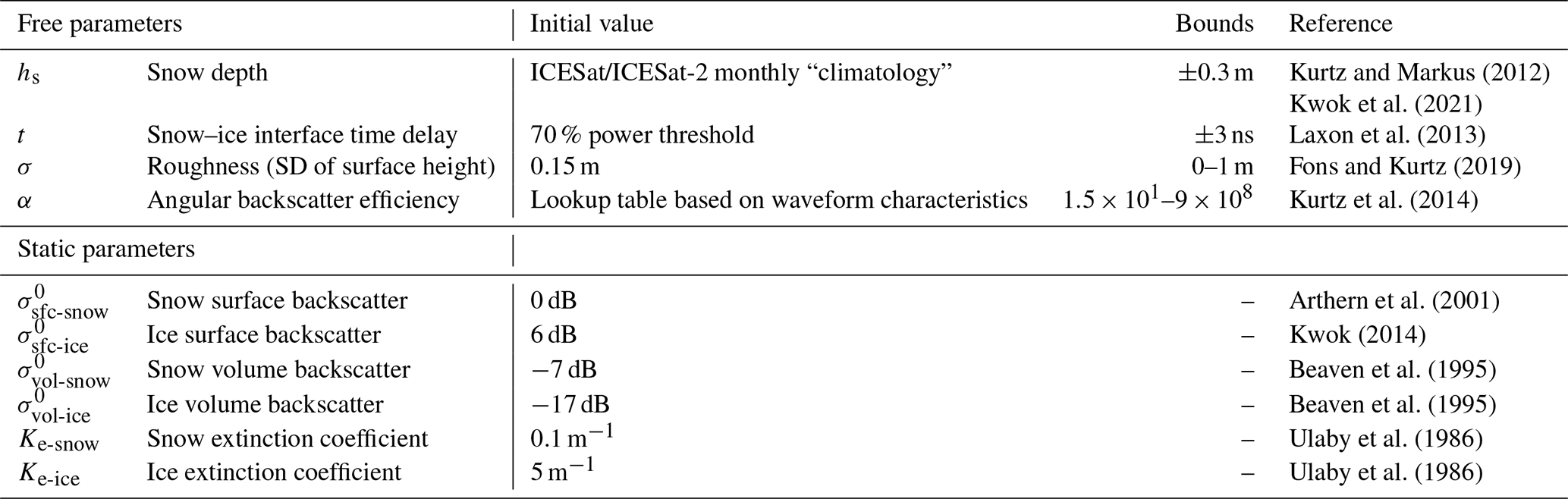
The next step involves fitting the modeled waveform to the actual CryoSat-2 waveform through a bounded trust-region Newton least squares optimization approach. Bounds are provided for each input parameter about the initial guess to constrain the optimization to best-guess physically realistic values for a given location or waveform shape (Table 1). While the bounds for σ and α are fixed values, the h_s and t bounds are given as plus or minus the initial value. For snow depth, the lower bound is set to zero if the lower bound of the provided range is negative. Each function evaluation adjusts the input parameters within the provided bounds, until a minimum residual between the modeled and actual waveforms is found, or until a maximum number of function evaluations (100) is reached. Waveforms are discarded if the maximum iteration number is reached, since it occurs infrequently (<0.5 % of waveforms). The output “fit parameters” provide estimates of the actual values of each parameter in the waveform model. The large assumptions are that (a) this waveform model accurately can represent a CryoSat-2 return from the sea ice surface, and (b) the fitting procedure, when initialized with physically realistic inputs and bounds, can find the global minimum optimization result as opposed to getting caught in a local minimum. Fit parameters are discarded if the result is a “poor fit”, which is described as having a squared norm of the residual greater than 0.3. These poor fits typically come from ambiguous returns with multiple peaks, usually brought on by off-nadir leads (Kurtz et al., 2014; Tilling et al., 2018) to which the wide footprint of CryoSat-2 is susceptible. In total, 14 % of all waveforms between 2010–2021 have been filtered out when using CS2WFA, predominantly coming from floe-type returns.

The output parameters of snow–ice interface tracking point and snow depth provide (when accounting for wave speed through the snowpack) the locations of the physical air–snow and snow–ice interfaces on the waveform as a function of radar return time. Retracking corrections are then calculated that relate these locations to the nominal tracking bin, provided in the CryoSat-2 data product as the “center range bin”. To retrieve the surface elevation (h_e), the retracking correction is added to a provided geophysical correction and the raw CryoSat-2 range. This retrieval is shown by

$$\begin{array}{}\text{(5)}& h_{\mathrm{e}}=A-R_{\mathrm{0}},\end{array}$$

where A is the altitude of the satellite center of gravity above the World Geodetic System 1984 (WGS84) ellipsoid, and R₀ is the range from the satellite to the surface, given by

$$\begin{array}{}\text{(6)}& R_{\mathrm{0}}=R_n+c_{\mathrm{r}}+c_{\mathrm{g}},\end{array}$$

where R_n is the raw range computed from the time delay to a reference point of the range window, c_r is the retracking correction, and c_g is the geophysical correction. Equation (5) results in the elevation of the surface above the WGS84 ellipsoid. These elevations can then be used to estimate freeboard.

It must be reiterated that the estimation of freeboard requires an estimate of the snow–ice interface elevation. As has been previously stated, empirical threshold retrackers typically assume the dominant scattering horizon is located at the snow–ice interface (and that the snow layer is mostly transparent at Ku-band frequencies), which can lead to an overestimation of the ice freeboard and is a primary reason behind low confidence in retrievals of ice freeboard over Antarctic sea ice (Paul et al., 2018). This physical retracking method does not contain the same assumption and instead uses the physical model and fitting method to estimate the actual snow–ice interface by accounting for attenuation of the signal in snow and ice layers. Therefore, it is hypothesized that this physical method better tracks that snow–ice interface compared to empirical approaches, which motivates the calculation of ice freeboard and snow depth. This idea is explored further in subsequent sections.

3.2 Estimating freeboard and snow depth

Once the snow–ice interface elevation is retrieved using the retracking procedure described above, it can be combined with the output snow depth (a fit parameter from the model) to estimate the air–snow interface elevation and snow freeboard. The air–snow interface elevation is found simply by adding the output snow depth to the snow–ice interface elevation. To estimate freeboard, the first step is determining the sea surface height (SSH). The elevation of all lead-type waveforms are averaged in running 10 km along-track segments and linearly interpolated, following Kwok et al. (2022). Lead segments are only calculated if at least three lead-type points exist within. This along-track SSH is then subtracted from every floe-type elevation, yielding a freeboard estimate for each floe-type point. Subtracting the SSH from the air–snow interface elevation results in a snow freeboard estimate, while that from the snow–ice interface results in an ice freeboard estimate. The output snow depth parameter gives our estimate of the snow thickness, which is equal to the air–snow interface elevation minus the snow–ice interface elevation. The effects of the snow layer on radar wave speed propagation are accounted for in the snow–ice interface retracking and the ice freeboard calculation, following Mallett et al. (2020) and shown in Fons et al. (2021).

Each floe-type waveform with a good fit has a snow freeboard, ice freeboard, and snow depth estimate, provided that a co-located 10 km sea surface height segment also exists. Estimates of freeboard and snow depth shown here are gridded onto the NSIDC 25 km polar stereographic grid, which is only done if a minimum of five waveforms exists within, following Kurtz et al. (2014).

3.3 Calculating sea ice thickness and volume

After obtaining estimates of sea ice freeboard and snow depth on sea ice, the thickness of the sea ice can be calculated by applying the hydrostatic assumption. This assumption follows that an object (in this case, snow-covered sea ice) immersed in a fluid will be buoyed with a force equal to that due to gravity. Combining the estimates of the freeboard and snow depth with estimates for the density of seawater, snow, and sea ice (as in Eqs. 1 and 2), one can calculate the thickness. We utilize the snow freeboard estimates to calculate thickness (i.e., Eq. 2) in the remainder of this work.

Typical values of sea ice and snow density used for Antarctic sea ice thickness calculation vary depending on the study. Most studies tend to use single, static density values across all seasons: ice density values tend to be around 915 to 917 kg m⁻³, while snow densities used tend to be 300 to 320 kg m⁻³ (Kern et al., 2016; Li et al., 2018; Kacimi and Kwok, 2020). Kurtz and Markus (2012) varied these values seasonally, based off in situ measurements collected around the continent. For ice density, they used 900, 875, and 900 kg m⁻³ for spring, summer, and autumn, respectively, based off the measurements collated in Worby et al. (2008) and Buynitskiy (1967). For snow density, they used 320, 350, and 340 kg m⁻³ for spring, summer, and autumn, respectively, following Massom et al. (2001).

In this work, we use seasonally varying snow and ice density values but interpolate them through time as an attempt to better capture a seasonal signal that is likely present as the sea ice evolves. To do this, we provide a “seasonal value” of density that is assigned to the approximate midpoint day of each season: 15 January for summer, 15 April for autumn, 15 July for winter, and 15 October for spring. For ice density, these seasonal values follow Kurtz and Markus (2012), Hutchings et al. (2015), and Buynitskiy (1967) and are set to 875 (summer), 900 (autumn), 920 (winter), and 915 (spring) kg m⁻³. The snow density values are set to 360 (summer), 350 (autumn), 330 (winter), and 310 (spring) kg m⁻³, following Massom et al. (2001) and Kurtz and Markus (2012). Then, these seasonal values are linearly interpolated between the midpoint dates, providing daily density estimates that are used in the thickness calculation. The interpolated densities are shown in Fig. 2. For the density of seawater, we use a static value of 1024 kg m⁻³.

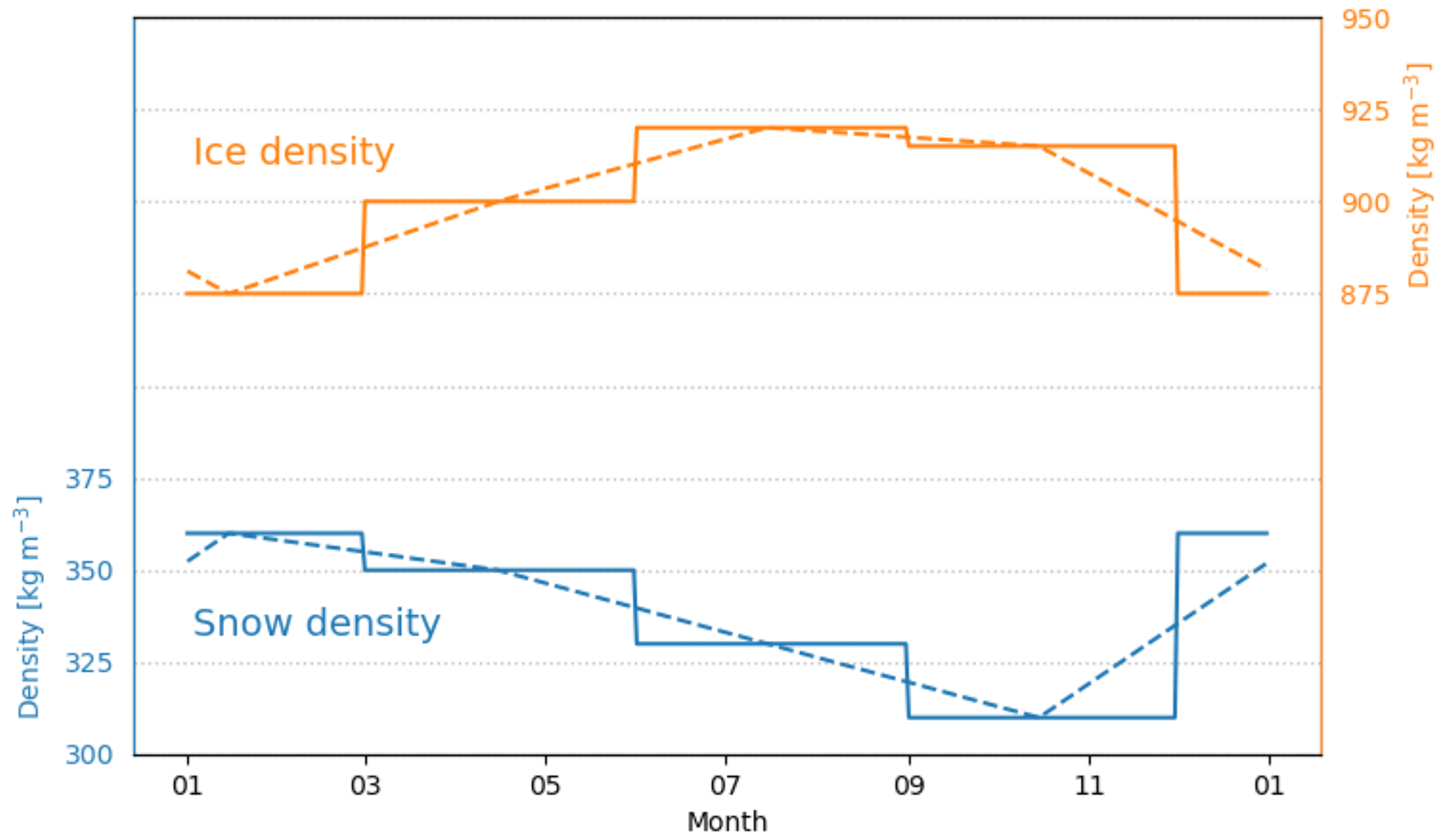
Figure 2 Sea ice (orange) and snow (blue) density values used in the thickness calculation. Solid lines are the fixed seasonal density values, while the dashed lines are linear interpolations between the midpoint dates and are used as daily density estimates in the thickness calculation.

Like freeboard and snow depth, thickness is also gridded using the NSIDC polar stereographic grid. Mean values shown herein are pan-Antarctic or regional averages and do not take the sea ice area into account (i.e., results shown are not area-weighted means). Volume is computed by multiplying basin- or region-average sea ice thickness by the areal coverage of sea ice pan-Antarctic or in each region, respectively.

For the freeboard, snow depth, thickness, and volume results given herein, both monthly and seasonally averaged data are shown from both pan-Antarctic as well as from individual regions. The seasons are broken up as follows: (1) summer, D–J–F; (2) autumn, M–A–M; (3) winter, J–J–A; and (4) spring, S–O–N. The regions are longitudinally demarcated as follows: (1) Ross Sea, 160–230^∘ E; (2) Amundsen–Bellingshausen seas (Am–Bel), 230–300^∘ E; (3) western Weddell Sea, 300–315^∘ E; (4) eastern Weddell Sea, 315–20^∘ E; (5) Indian Ocean, 20–90^∘ E; and (6) Pacific Ocean, 90–160^∘ E. These regions are shown in Fig. 4.

3.4 Estimating uncertainty in sea ice thickness and volume retrievals

In this work, an estimate of the uncertainty in the thickness and volume measurements are provided through a Gaussian error propagation method (following Spreen et al., 2009; Kern and Spreen, 2015; Petty et al., 2020). The total uncertainty in a thickness measurement comes from a combination of random and systematic uncertainties. Random uncertainties in thickness measurements can be calculated (Petty et al., 2020); however, because they are random, we assume they decrease substantially when many individual thickness measurements are averaged together. Since thickness results in this study are shown only over large scales and averaged monthly to a 25 km grid, we assume the random uncertainty becomes negligible basin wide and do not explicitly calculate it here. Future work involving along-track thickness estimates and validation would necessitate a calculation of random uncertainty as well as an estimate of the uncertainty brought on by the fitting procedure itself.

Instead, an estimate of the systematic uncertainty at the grid-cell-scale is given here. We assume these uncertainties are correlated and represent bias in the measurement and therefore cannot be reduced through averaging (Ricker et al., 2014). Here, the systematic uncertainty is estimated following Petty et al. (2020) where

$$\begin{array}{}\text{(7)}& \begin{array}{rl}{\mathit{\sigma }}_{\mathrm{hi}-\mathrm{fs}}^{\mathrm{2}}=& {\mathit{\sigma }}_{\mathrm{hs}}^{\mathrm{2}}{\left({\displaystyle \frac{{\mathit{\rho }}_{\mathrm{s}}}{({\mathit{\rho }}_{\mathrm{w}}-{\mathit{\rho }}_{\mathrm{i}})}}-{\displaystyle \frac{{\mathit{\rho }}_{\mathrm{w}}}{({\mathit{\rho }}_{\mathrm{w}}-{\mathit{\rho }}_{\mathrm{i}})}}\right)}^{\mathrm{2}}\\ & +{\mathit{\sigma }}_{{\mathit{\rho }}_{\mathrm{s}}}^{\mathrm{2}}{\left({\displaystyle \frac{h_{\mathrm{s}}}{({\mathit{\rho }}_{\mathrm{w}}-{\mathit{\rho }}_{\mathrm{i}})}}\right)}^{\mathrm{2}}+{\mathit{\sigma }}_{{\mathit{\rho }}_{\mathrm{i}}}^{\mathrm{2}}\\ & {\left({\displaystyle \frac{h_{\mathrm{fs}}{\mathit{\rho }}_{\mathrm{w}}}{({\mathit{\rho }}_{\mathrm{w}}-{\mathit{\rho }}_{\mathrm{i}}{)}^{\mathrm{2}}}}+{\displaystyle \frac{h_{\mathrm{s}}{\mathit{\rho }}_{\mathrm{s}}}{({\mathit{\rho }}_{\mathrm{w}}-{\mathit{\rho }}_{\mathrm{i}}{)}^{\mathrm{2}}}}-{\displaystyle \frac{h_{\mathrm{s}}{\mathit{\rho }}_{\mathrm{w}}}{({\mathit{\rho }}_{\mathrm{w}}-{\mathit{\rho }}_{\mathrm{i}}{)}^{\mathrm{2}}}}\right)}^{\mathrm{2}}.\end{array}\end{array}$$

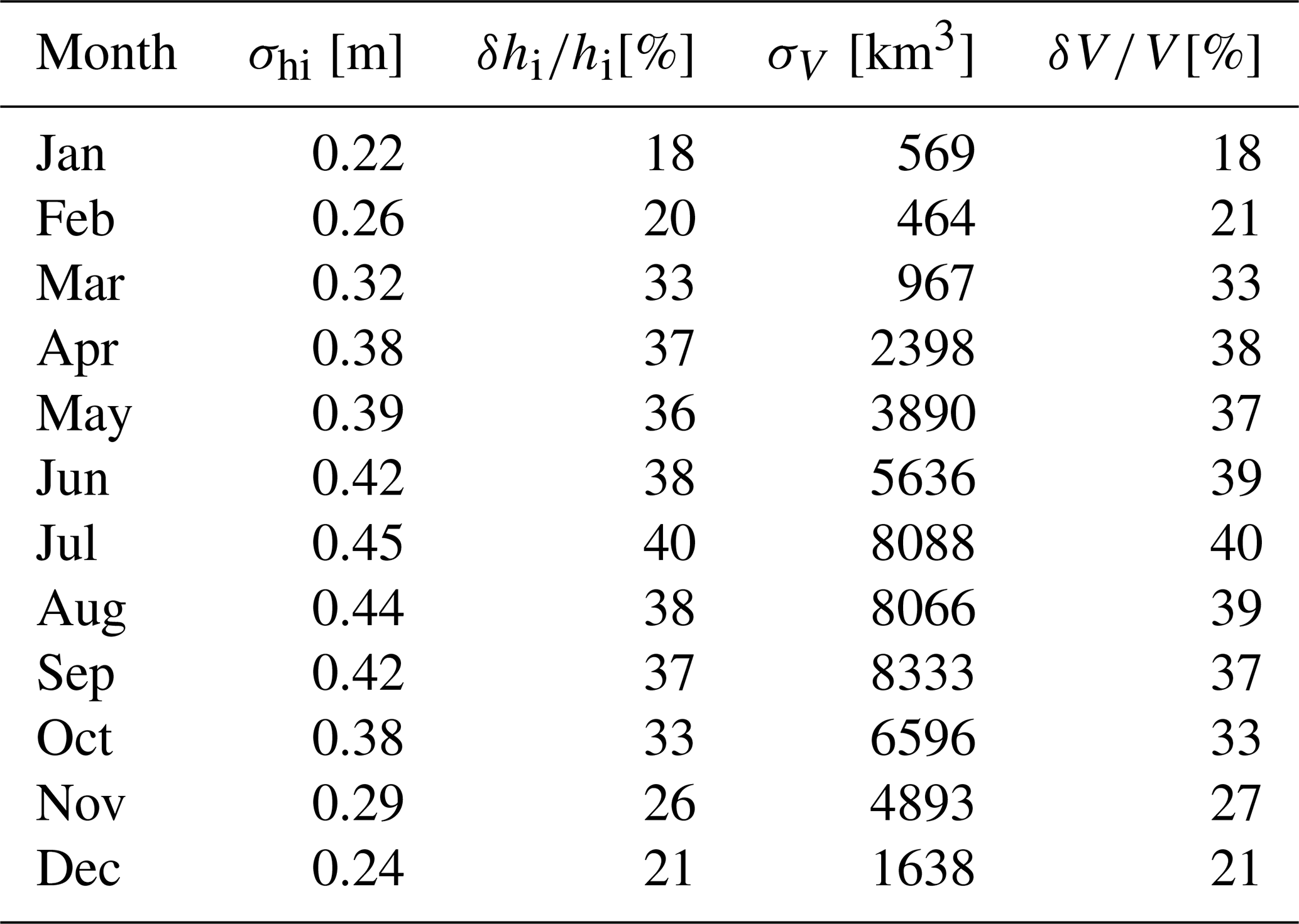
In Eq. (7), σ_hi−fs is the uncertainty in sea ice thickness estimated using snow freeboard (Eq. 2); h_s is the snow depth; h_fs is the snow freeboard; and s, w, and i represent the density (ρ) and uncertainty (σ) of snow, seawater, and sea ice, respectively. The snow depth uncertainty σ_hs is taken as the standard deviation of snow depth measurements with each 25 km grid cell, following Petty et al. (2020). Densities of snow (ρ_s), ice (ρ_i), and water (ρ_w) are set to the values given in Kurtz and Markus (2012), with the uncertainty in the snow density (σ_ρs) taken as 50 kg m⁻³ and the uncertainty in the ice density (σ_ρi) taken as 20 kg m⁻³. The uncertainty in the seawater density is assumed to be negligible and is not included in this calculation (Kurtz and Markus, 2012; Kern et al., 2016; Li et al., 2018). Monthly average 25 km grids of snow depth (h_s) and snow freeboard (h_fs) are used in the uncertainty calculation, and therefore uncertainty estimates are provided for each grid cell basin wide. Monthly average thickness uncertainty values range from around 22 to 45 cm and are given (basin wide) in Table 2.

Table 2 Monthly pan-Antarctic sea ice thickness (h_i) and volume (V) uncertainty found in this study, shown both as absolute (σ) and fractional (δ) values. All values are 2010–2021 averages.

An estimate of the volume uncertainty is also provided but is done so in a simplistic way compared to other methods over Arctic sea ice (Tilling et al., 2018). Here, a Gaussian error propagation approach is used to combine the uncertainty due to sea ice thickness and sea ice area, the two components that make up the volume calculation. This is provided as an initial volume uncertainty estimate until more information on the uncertainty relating to snow depth and snow/ice density from Antarctic sea ice is known.

This estimated volume uncertainty is given by

$$\begin{array}{}\text{(8)}& {\displaystyle \frac{\mathit{\delta }V}{\left|V\right|}}=\sqrt{{\left({\displaystyle \frac{\mathit{\delta }{h}_{\mathrm{i}}}{h_{\mathrm{i}}}}\right)}^{\mathrm{2}}+{\left({\displaystyle \frac{\mathit{\delta }A}{A}}\right)}^{\mathrm{2}}},\end{array}$$

where $\mathit{\delta }V/\left|V\right|$ is the monthly average sea ice volume fractional uncertainty, $\mathit{\delta }{h}_{\mathrm{i}}/h_{\mathrm{i}}$ is the sea ice thickness fractional uncertainty, and $\mathit{\delta }A/A$ is the fractional uncertainty in sea ice area. In this study, a conservative fractional uncertainty value for sea ice area of 5 % is used, following Spreen et al. (2009). The fractional uncertainty in thickness ($\mathit{\delta }{h}_{\mathrm{i}}/h_{\mathrm{i}}$) is found by dividing the thickness uncertainty grid by the mean thickness grid and computing the basin-wide average. The right-hand side of Eq. (8) provides a fractional combined uncertainty in sea ice volume. Multiplying this fractional uncertainty with the mean volume estimate yields a quantitative sea ice volume uncertainty. This uncertainty ranges generally between 18 %–40 % of the total sea ice volume (Table 2) and is dominated by the uncertainty in thickness. Once again, these thickness and volume uncertainty values are simply first estimates used to constrain the estimates in the context of the observed interannual variability, and we acknowledge there are limitations to these calculations. These uncertainty values are provided for the pan-Antarctic in Table 2.

4 Results

The methodology described in Sect. 3 was applied to all CryoSat-2 data collected over the Southern Ocean from the beginning of the mission in July 2010 until August 2021, resulting in over 11 years of data. This time period is hereafter referred to as the “CryoSat-2 period”. In this section, we show results from CS2WFA, comparisons with other data sets, and observed changes over the CryoSat-2 period. The following sections cover snow freeboard (Sect. 4.1), snow depth (Sect. 4.2), thickness (Sect. 4.3), volume (Sect. 4.4), and intra-decadal changes in thickness and volume (Sect. 4.5).

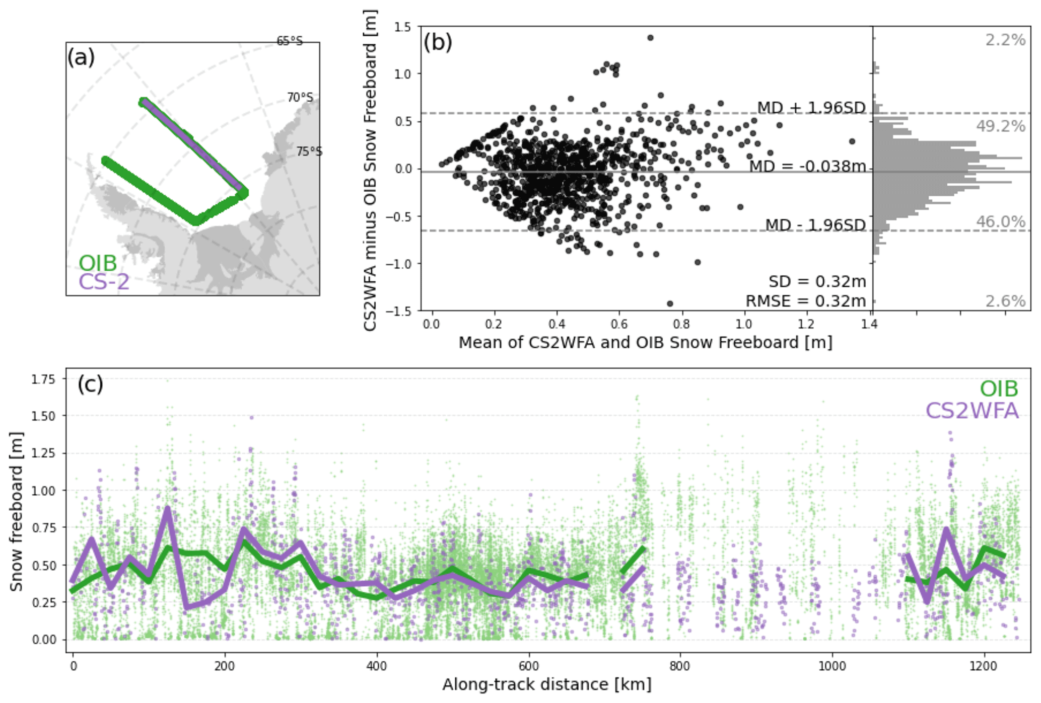
Figure 3 Comparison of the CS2WFA-retrieved snow freeboard to that from OIB, for the October 2010 underflight in the Weddell Sea. Panels include (a) a map of the overlapping orbit; (b) Tukey mean-difference plot comparing CS2WFA to OIB, where OIB points are averaged to the same along-track resolution as CryoSat-2; and (c) a 1.2+ km profile of the overlapping segment. Small points are full-resolution estimates from CS2WFA (purple) and OIB (green), while lines are 25 km binned averages. Note that lines are only drawn if at least four points exist in successive 25 km bins. The mean difference (MD), standard deviation of differences (SD), and root mean square error (RMSE) are shown in (b).

4.1 Snow freeboard

The retrieved snow depth is added to the snow–ice interface tracking point to estimate the air–snow interface elevation and, when combined with the SSH, the snow freeboard. The snow freeboard results from CS2WFA were presented extensively in Fons et al. (2021), and therefore readers are directed there for full snow freeboard results and comparisons to ICESat-2. Here, we provide an independent comparison to OIB snow freeboard data, collected from an October 2010 OIB underflight of the CryoSat-2 orbit in the Weddell Sea.

Figure 3 shows a comparison of the CS2WFA estimates to that from OIB. Agreement is good overall, with a CS2WFA thin bias of under 4 cm on average. When averaging OIB estimates to the same along-track resolution as CryoSat-2 (Fig. 3b), the differences are normally distributed with few points falling outside of 2 standard deviations of the mean difference. While OIB is thicker on average, there looks to be a thick bias from CS2WFA for snow freeboards greater than 0.8 m. Additionally, for thinner freeboards, there appears to be a higher concentration of points spread further from parity, which could signal CS2WFA recording more positive freeboards where OIB finds zero freeboards. Standard deviation of differences and root mean square error are both 32 cm. Figure 3c shows a general ability of CS2WFA to capture the large-scale along-track freeboard profile, with some exceptions (e.g., around ∼ 180 km along track). It is clear from Fig. 3c that the sampling resolutions between the two instruments are markedly different, which likely impacts the comparison shown here. Further discussion on the independent comparisons are given in Sect. 5.1.

4.2 Snow depth on sea ice

The output snow depth parameter from the fit waveform model provides along-track snow depth on sea ice for the duration of the CryoSat-2 period. This section showcases a snow depth comparison as well as seasonal patterns in the snow depth distribution.

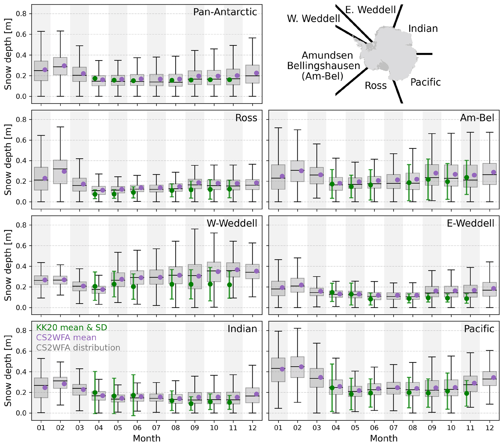
Figure 4 Comparison of the CS2WFA-retrieved snow depth to that from KK20 for each region in the year 2019. Boxplots are from the CS2WFA data for each month, where the boxes show the interquartile range (IQR), whiskers show 1.5 times the IQR, horizontal lines are the medians, and purple dots are the mean values. Green points and whiskers represent the mean value and standard deviation from KK20. In the pan-Antarctic panel, the means are simply an average of all the individual region means and therefore do not include standard deviations.

The lack of reliable in situ data involving snow depth on Antarctic sea ice poses a challenge when attempting to validate snow depth retrievals from CryoSat-2. Here, snow depth estimates from KK20 are used as a point of comparison for region-scale snow depth retrievals from CryoSat-2. Figure 4 shows a regional comparison between CS2WFA and KK20 snow depths for the year 2019. Data from KK20 are only provided in April–November and are missing in July due to a gap in data collection from ICESat-2. Differences are generally within 5 cm, though can be larger in regions where snow (and ice) thickness is typically greatest, especially the western Weddell sector. In other regions, KK20 mean snow depths almost always fall within the CS2WFA interquartile range. The two data sets exhibit a similar seasonal pattern; however, KK20 snow depths exhibit less growth over the year, as the change from ∼ June to November is generally smaller than that from CS2WFA.

Monthly differences in pan-Antarctic snow depth (CS2WFA minus KK20) range from 0.2 cm in April to 7.5 cm in November. There are some caveats however. While these measurements both use CryoSat-2 data to estimate the snow–ice interface elevation, KK20 also uses ICESat-2 data and only collects snow depths within ±10 d from a valid ICESat-2 freeboard measurement. Therefore, it must be noted that each month in this comparison involves different amounts of data between the two methods, which could explain some of the differences observed. This is especially true in November, when KK20 only uses the first 2 weeks of ICESat-2 data, while these CS2WFA data come from the whole month. Despite some of these differences, the observed similar seasonality and small mean differences in the snow depths between both data sets is encouraging. However, validation data – as opposed to intercomparison data and especially in austral summer – would be useful to better assess the snow depths retrieved from both of these methods.

Figure 4 also gives insight into the regional variation in summer snow depths retrieved from CS2WFA. It is important to note that different regions each contain different numbers of grid cells, which surely impacts these direct comparisons. In all sectors except the western Weddell sector, the thickest average snow depths are found to occur in summer months (usually February). This finding is consistent with what is found in Worby et al. (2008) and is hypothesized to be due to the fact that the older ice near the coast that survives summer melt has had more time for snow accumulation and therefore thicker snow depths. Additionally, the regions with the largest difference in snow depth in summer compared to other months (i.e., Pacific, Indian, Ross) experience the largest ice extent change between winter and summer, which could explain these substantial differences in the regional averages.

In the western Weddell, some of the thinnest average snow depths occur in the late summer (F–M). This finding is seemingly counterintuitive given the behavior of the other regions; however, this was also observed by Worby et al. (2008). One possible explanation could be due to the presence of surface melting of the snow layer that can act to reduce snow depths and/or potentially impact retrievals in this region and season. Markus and Cavalieri (1998) found that surface melt in summer months in this region can occur – due in part to the more-northern location compared to other regions – and found that this melt can complicate passive microwave returns. Here, it is possible that surface melt could lead not just to thinner snow depths, but also could lead to erroneous CryoSat-2 waveform classification, as melt-affected floe points may appear more specular in radar returns. This surface melt could cause misclassification of sea ice returns, which could impact the SSH and retrieved snow–ice interface elevations, potentially leading to higher-than-expected snow–ice interface elevations and anomalously thin snow depths. Another explanation is that the yearly change in ice area in the western Weddell is smaller than in any other region. This consistency in ice extent means that the region-averaged seasonal cycle would be controlled more so by actual changes in the snow depth (e.g., from surface melt or accumulation) than by changes in the ice extent that get averaged into the regional mean (e.g., from new ice formation that has near-zero snow).

The 2010–2021 mean snow depth on Antarctic sea ice for each season is given in Fig. 5, along with the basin-wide snow depth distribution for all grid cells between 2010 and 2021. Most notably, these spatial patterns and distributions appear more realistic (based off of other estimates from Markus and Cavalieri, 1998, Kern and Ozsoy-Çiçek, 2016, and Kacimi and Kwok, 2020) than what was attempted in Fons and Kurtz (2019), signalling that the model and retrieval improvements made in Fons et al. (2021) had a substantial – and beneficial – effect on the snow depth retrievals. In Fig. 5, one can see the seasonal growth in snow thickness, as any given region shows an increase from autumn to winter to spring. This growth is expected throughout the year and is similar to what is found in Kern and Ozsoy-Çiçek (2016) between winter and spring. Also, the distributions show the impact of ice extent on the basin-averaged snow depth, as they shift from broad (little extent but thicker snow) to thin (large extent with thinner snow on average). Pan-Antarctic snow depths range between 16 and 25 cm on average, with the thickest basin-averaged snow depths in summer (consistent with the comparisons shown in Fig. 4). Standard deviations of snow depth range between 9.4 and 12.9 cm.

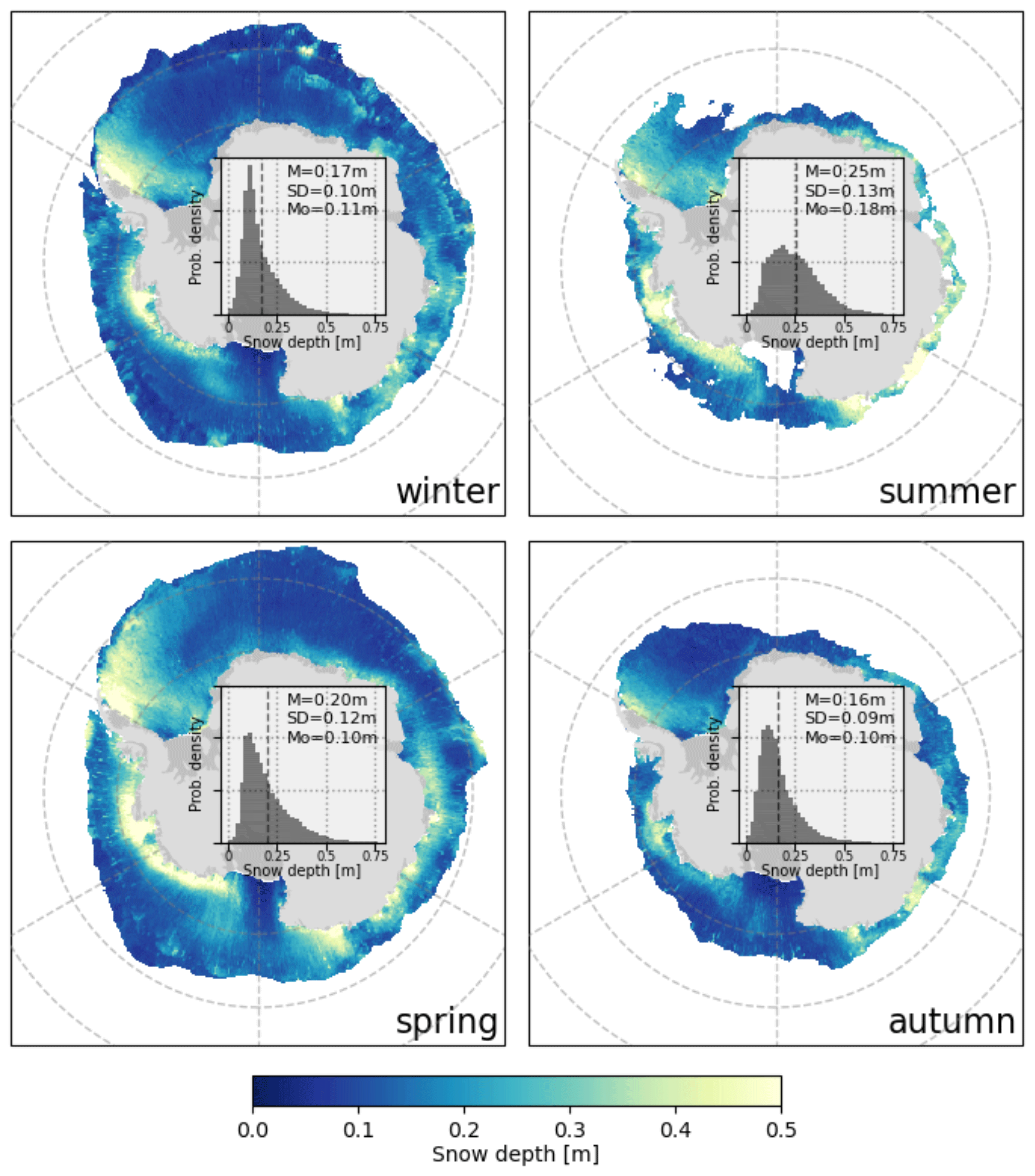
Figure 5 Seasonal average (July 2010–August 2021) maps and distributions of snow depth from CS2WFA. Histogram bin sizes are 0.02 m. The dashed line represents the mean value, and the mean (M), standard deviation (SD), and mode (Mo) values are given.

Overall, the retrieved CS2WFA snow depths show reasonable spatial and temporal distributions that generally compare with estimates from KK20, despite the sampling differences. Further snow depth comparisons with the extended ASPeCt data set (Kern, 2020) are shown in Sect. 5.1, accompanying a more detailed discussion on the comparisons performed here. In the next section, these snow depths are combined with snow freeboard estimates (detailed in Fons et al., 2021 and shown in Sect. 4.1) to estimate sea ice thickness.

4.3 Sea ice thickness

The retrieved snow freeboards and snow depths shown above are used in Eq. (2) to calculate the sea ice thickness. Here, estimates of Antarctic sea ice thickness derived from CryoSat-2 from the years 2010–2021 are shown.

The monthly mean Antarctic sea ice thickness distributions and spatial patterns from 2010 to 2021 are given in Fig. 6. Basin-wide thicknesses are largest in February (1.26 m), when ice extent is at a minimum, and lowest in March (0.95 m), when new ice has began to form. Monthly standard deviations range from 59 to 78 cm. The summer distributions tend to be broader than other months, though all months exhibit a singular mode. The spatial pattern follows closely with that of snow depth (Fig. 5), with the largest thicknesses being found in the western Weddell sector, as well as along the coast in the Am–Bel and Pacific sectors, while thinner ice tends to be found away from the coast in the eastern Weddell, Indian, and Ross sectors. These values tend to be thicker than those observed in previous studies (e.g., Worby et al., 2008), which is discussed later in this section.

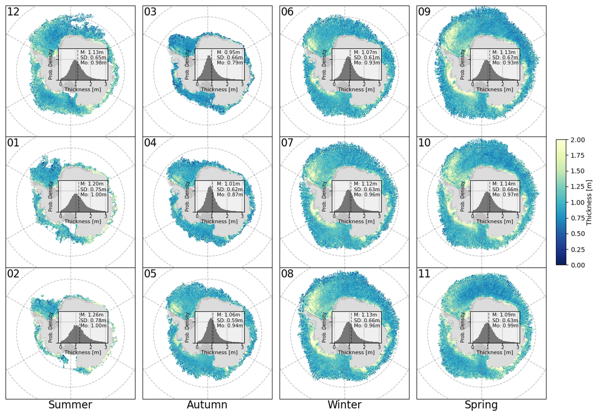
Figure 6 Monthly average (July 2010–August 2021) maps and distributions of sea ice thickness from CS2WFA, arranged in columns by season. Histogram bin sizes are 0.05 m. The dashed line represents the mean value, and the mean (M), standard deviation (SD), and mode (Mo) values are given.

When averaged over all years, the monthly thickness distributions in Fig. 6 tend to mask some of the variability present both regionally and seasonally. To investigate this variability, Fig. 7 gives thickness distributions broken down by region and season. The regional variability is apparent: the Pacific, western Weddell, and Am–Bel sectors showcase broader distributions (density ⪅1) with thicker mean values, while the other regions show a narrower distribution (probability density ⪆1) and slightly thinner means. The largest seasonality within a region is found in the Pacific sector, where the summer ice thickness is noticeably thicker than the other seasons, owing to the low extent present during this season. Like what was found in the snow depth results, the western Weddell summer shows the thinnest ice thickness of all seasons. This result once again matches what was found in Worby et al. (2008) and is likely due in part to the relatively stable seasonal ice extent in this region that shows the basal melt occurring in summer and contributes less to a “thickening” by way of averaging over a low ice extent.

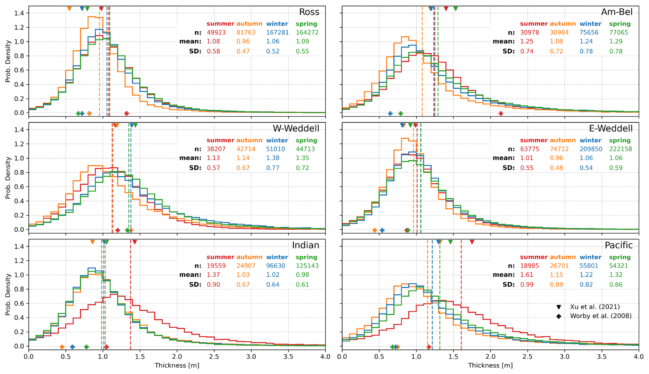
Figure 7 Seasonal thickness distributions from each of the six regions covering 2010–2021. Red represents summer, orange represents autumn, blue represents winter, and green represents spring, where the vertical dashed line gives the mean value. The number of grid cells, mean, and standard deviations of the distributions are given. Bin sizes are 0.1 m. Crosses on the bottom and triangles on the top mark the seasonal and regional mean values from Worby et al. (2008) and Xu et al. (2021), respectively.

Crosses and triangles in Fig. 7 on the bottom and top show the seasonal/region mean values given from the ASPeCt data set in Worby et al. (2008) (1981–2005; total level and ridged thickness) and from ICESat/ICESat-2 in Xu et al. (2021) (2003–2008, 2018–2020), respectively. In most regions, these CS2WFA thicknesses tend to estimate thicker ice than Worby et al. (2008) but are generally comparable to Xu et al. (2021). Despite some differences between the data sets, a few similarities can be seen. First, mean thicknesses in the western Weddell sector agree well between all three data sets. Additionally, all three find the Indian and Pacific regions to have the thickest sea ice in the summer, with Worby et al. (2008) also showing the thickest sea ice in summer in the Ross and Am–Bel regions. Both Worby et al. (2008) and Xu et al. (2021) find summer to be the thinnest season in the western Weddell sector, matching what we show with CS2WFA. Further discussion on these comparisons – including the inherent biases in the ship-based observations – and a more detailed comparison with extended ASPeCt data are given in Sect. 5.1.

Another interesting feature in the seasonal distributions is the perceived lack of seasonal variability in some regions. Some sectors showcase more seasonal variation in the distributions, while others show a very similar mode and distribution shape in all seasons. This lack of seasonality contrasts what is found in Arctic sea ice, where a clear seasonal cycle exists in the thickness distributions (Petty et al., 2020). One contributing factor is the fact that these distributions are created from the entire 11-year record. When looking at an individual region and season over time (Fig. 8), one can see much larger variability in the regional and seasonal mean values.

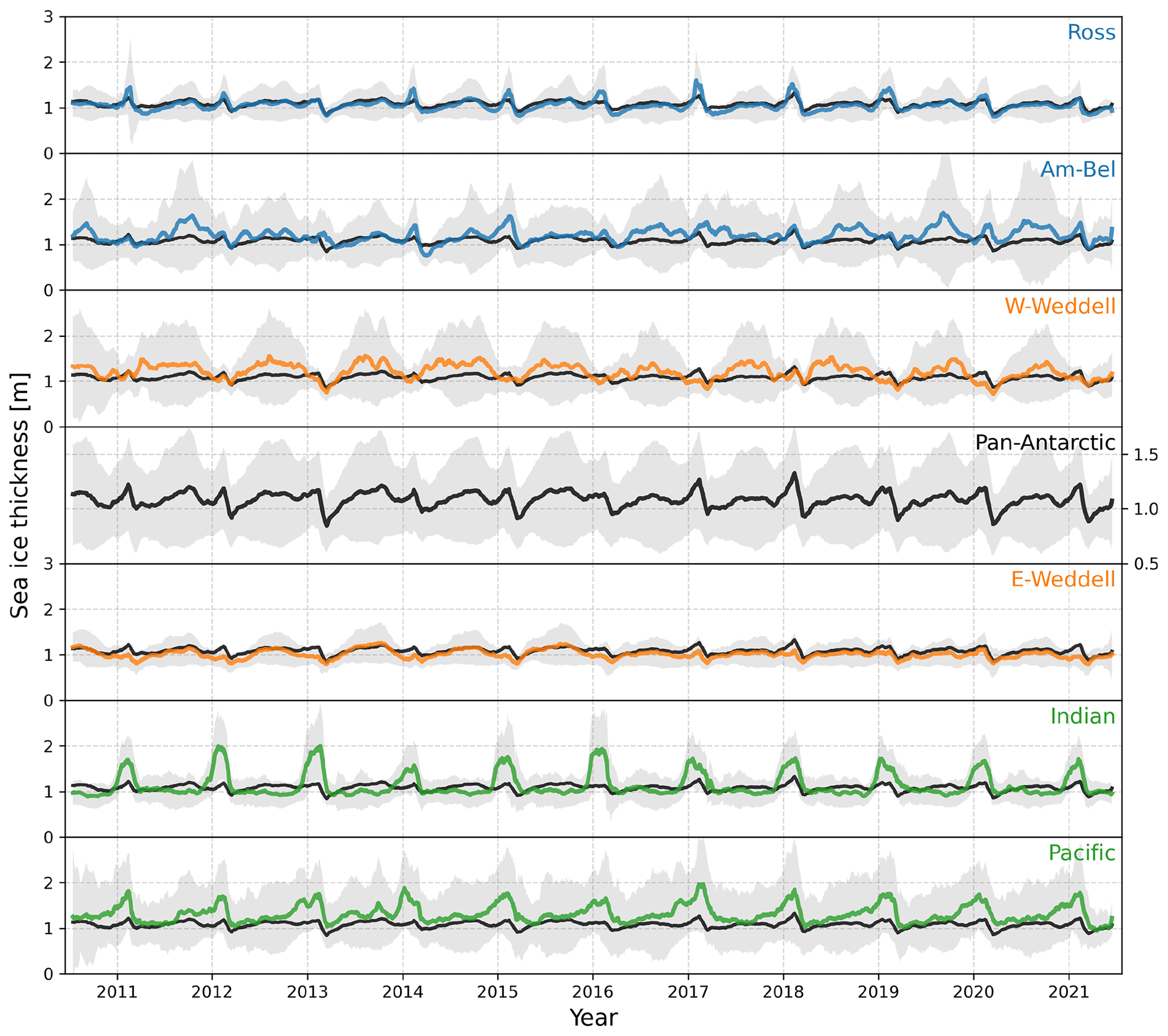
Figure 8 Time series of Antarctic sea ice thickness covering the entire CryoSat-2 period 2010–2021. The black line represents the pan-Antarctic average and is shown by itself and with all individual regions (panels). The shaded regions show the estimated uncertainty in the pan-Antarctic and in each individual region, which is computed as an average uncertainty of all grid cells of each region. Note the scales are the same for all panels except for the pan-Antarctic panel, which is zoomed in to better show changes over time.

Figure 8 shows the pan-Antarctic sea ice thickness (solid black line) averaged as a 31 d rolling mean, as well as from individual sectors (panels) from July 2010 until August 2021. When viewed in this sense, a clear seasonal cycle of thickness emerges: pan-Antarctic-averaged thickness increases through austral summer, reaching a maximum around February with the minimum in sea ice extent (Parkinson, 2019). The pan-Antarctic average thickness then falls in March when new ice forms. After, there is a gradual thickening through autumn and winter as both ice extent and growth (driven by basal thickening and snow–ice formation) continues. This thickening slows and switches to a slight thinning by the middle and end of spring, as growth slows and melt begins basin wide. The thickness only increases on average once the thinnest ice melts entirely in the beginning of summer, leaving only the thickest ice present near the continent. This cycle continues each year.

While the time series in Fig. 8 shows the general seasonal cycle described above, there does exist some variability in the magnitude of the pan-Antarctic thickness. For example, the February peaks in ice thickness vary between less than 1.2 and more than 1.3 m on average, while the March minima also vary between ∼ 0.85 and 1.05 m. This variation can be much larger amongst individual regions.

Compared to other studies, the mean thickness values shown here appear, at first glance, to be slightly thicker than expected, especially in months of new ice growth where one would expect much of the ice cover to be below 1 m. Plus, other methods showed thinner results: Kurtz and Markus (2012) found mean values below 1 m for all seasons, Worby et al. (2008) found thinner annual and seasonal means from ship-based observations (Fig. 7), and Maksym and Markus (2008) showed thinner passive microwave-based thicknesses. However, these methods each contain caveats that help to explain the thinner results. Kurtz and Markus (2012) used the ZIF assumption, while Maksym and Markus (2008) only showed level ice thickness results, both of which are expected to produce thinner estimates. The ship-based observations from Worby et al. (2008) are often thought to be biased thin, due to the ships preferentially traveling through thinner ice (discussed further in Sect. 5.1). Other satellite-based studies found thicknesses comparable with – and even thicker than – these CS2WFA results. Kern et al. (2016) compared different ICESat approaches and found ice plus snow pan-Antarctic thicknesses to be around 0.25 and 0.65 m thicker than CS2WFA in spring and autumn, respectively. As shown in Fig. 7, Xu et al. (2021) found regional and seasonal thickness values comparable to these from CryoSat-2. KK20 acknowledged that their estimates seem high and included multiple estimates of thickness to “correct” for the anomalously thick results, introducing correction factors of δ=3 cm and δ=6 cm that adjusted the snow depth due to displacement of the scattering surface. These CS2WFA thickness estimates are slightly thinner than what was estimated by KK20 and closer to their δ=6 cm values. While it is possible that these satellite-based methods are too high – potentially from anomalous snow–ice interface tracking, surface-type mischaracterization, differing assumptions, or other factors – it is also possible that the Antarctic sea ice thickness distribution is simply thicker than previously assumed (Williams et al., 2015) and that ship-based observations and ZIF satellite estimates simply underestimate the actual thickness. More discussion on the “actual” thickness of Antarctic sea ice is provided in Sect. 5.

4.4 Sea ice volume

For each month of sea ice thickness data shown above, the monthly mean sea ice volume is also computed. This is done by multiplying the sea ice areal coverage in the basin or region by the mean ice thickness. A time series of volume is given in Fig. 9, where the pan-Antarctic total volume (black line) is broken down into contributions from the various sectors. The sea ice volume varies substantially within a year, ranging from around 2500 to around 20 000 km³. The Ross and eastern Weddell sectors contribute the largest percentage of volume in the winter and autumn seasons (when area is greatest), while the western Weddell sector tends to contribute most to the spring and summer pan-Antarctic sea ice volume. These values compare overall to the volume estimates put forth in KK20, both in the basin-wide sense as well as in the individual regions.

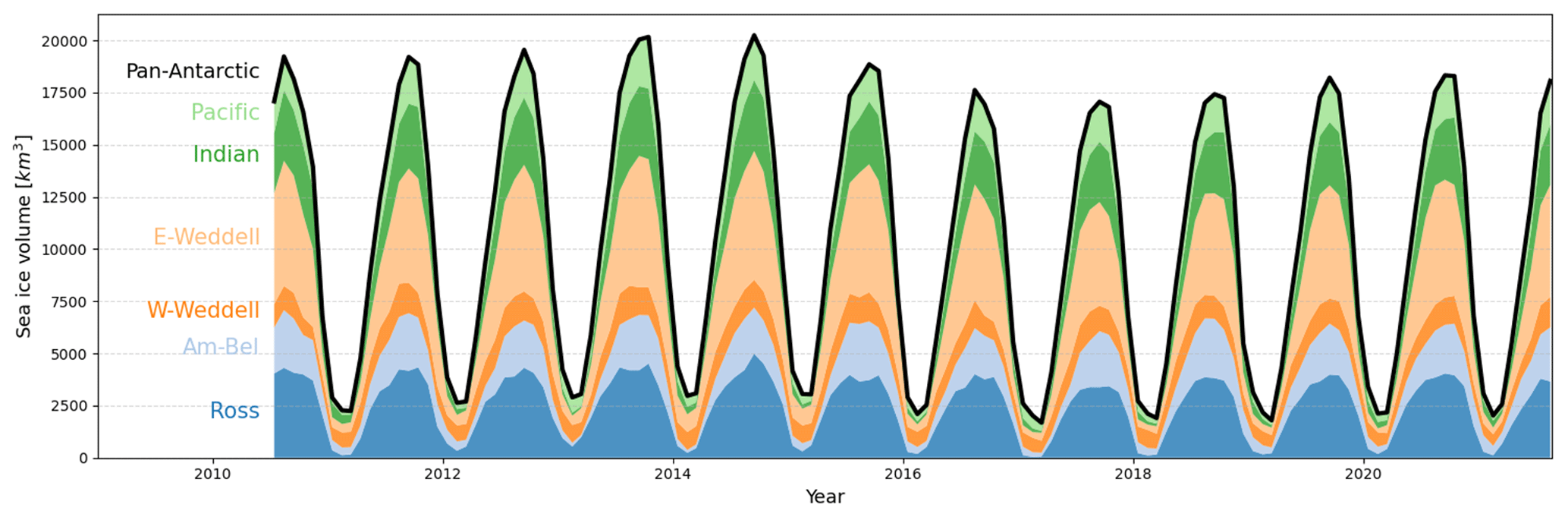
Figure 9 Time series of Antarctic sea ice volume covering the entire CryoSat-2 period 2010–2021. The dark black line represents the pan-Antarctic total volume, shown as the sum of the individual regions.

The time series of volume in Fig. 9 follows closely with the time series in sea ice extent shown in Parkinson (2019), which makes sense given that the pan-Antarctic sea ice volume calculation is dominated in magnitude by the sea ice area. This similarity is evident during the volume maximum in 2014 and the volume minimum in 2017, which correspond to the largest and smallest Antarctic sea ice extents, respectively, found over the satellite record (Parkinson, 2019). There is clearly more interannual variability in months of greater sea ice volume (August–October) than in months of less volume (January–March).

4.5 Intra-decadal changes in sea ice thickness and volume

Here, we present changes per year in the Antarctic sea ice thickness and volume over this 11-year record. These trends are calculated using the data we have available from CS2WFA and do not necessarily represent longer-term trends in the Antarctic sea ice pack. This is especially true given that the Southern Ocean is influenced by multi-decadal oscillations that can drive changes in the sea ice over longer timescales. Until a longer time series can be attained, we present just the changes in the ice pack between 2010 and 2021 from CS2WFA.

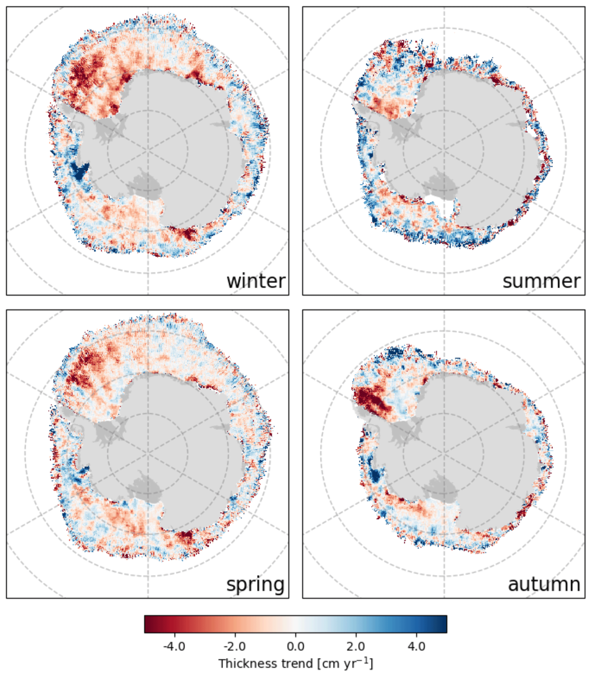
Figure 10 Seasonal changes in Antarctic sea ice thickness between 2010–2021. Red values indicate thinning, while blue values indicate thickening over time.

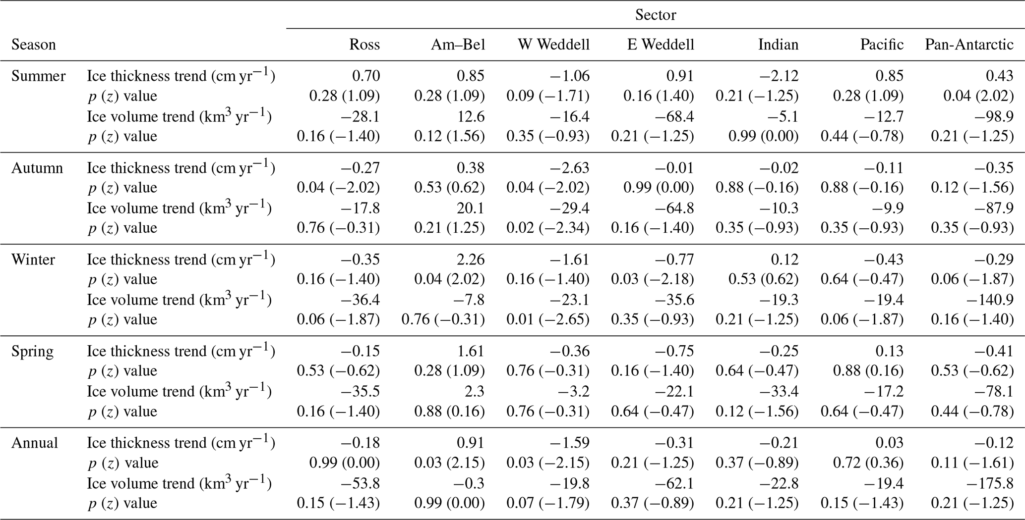
Figure 10 shows the change in thickness between 2010–2021 for each 25 km grid cell basin wide. The slope of the regression line of each grid cell time series is calculated using the Theil–Sen estimator and is only reported if a respective grid cell contains at least 4 years of data. Four years was chosen as a simple way to ensure multiple data points in each grid cell; however, there is no constraint on the part of the CryoSat-2 period from which the 4 years come. To reduce noise in the trend data, sea ice thickness maps are first smoothed with a 5 × 5 grid cell Gaussian kernel filter, which corresponds to an effective size of 125 × 125 km (following Kurtz and Markus, 2012). The region-average Theil–Sen slopes are given in Table 3. Also given in Table 3 are the reported p values, which come from the Mann–Kendall test of the null hypothesis that there is no monotonic trend in the time series, as well as z values indicating the normalized Mann–Kendall score, where negative values indicate a negative trend and vice versa. These values are presented as objective statistics for the data we have available, covering 2010–2021.

One can initially see a lot of variation in the trends around the continent in all seasons; however, some areas exhibit larger magnitude changes. In autumn, most of the western Weddell sector exhibits a strong thinning over this time period, with a region mean of over 2.6 cm yr⁻¹, which is larger than the trends observed here in other seasons (1 to 1.6 cm yr⁻¹ in summer and winter and 0.3 in spring). In winter, there is a large area of thinning predominantly in the eastern Weddell Sea, corresponding to regional changes observed of −0.8 cm yr⁻¹ on average (Table 3). There is also an area of thickening in the Am–Bel region (2.3 cm yr⁻¹), which agrees with the observation-based trends in Garnier et al. (2022) and modeled trends shown in Holland (2014) for this region, despite covering different time periods. In summer, each region shows a slight thickening on average, with the exception of the Indian and W Weddell sectors, which show thinning of 2.1 and 1.1 cm yr⁻¹, respectively. This contrasts Xu et al. (2021), who found summer thinning in all regions, albeit covering a different time range and using different instruments. The pan-Antarctic trend in the summer between 2010 and 2021 is found to be 0.4 cm yr⁻¹. When considering annual average changes over this time period, the W Weddell region shows a thinning of around 1.6 cm yr⁻¹, while the Am–Bel region shows a thickening of 0.9 cm yr⁻¹. Both of these trends agree with Garnier et al. (2022), who found similar negative and positive trends, respectively, over this time period. Once again, these trends are presented simply to show the changes CS2WFA finds in the ice pack between 2010–2021 and do not necessarily represent longer, multi-decadal trends in Antarctic sea ice.

Table 3 Antarctic sea ice thickness trends from 2010–2021 broken down by region and season. Trends give the slope of the regression line found using the Theil–Sen estimator. The p and z values of the reported trends are also given, where p values come from the Mann–Kendall trend test, and z values are the normalized Mann–Kendall score.

5 Discussion

Overall, the results presented above suggest that the CS2WFA method can provide reasonable estimates of snow depth on sea ice, sea ice freeboard, sea ice thickness, and sea ice volume. Agreement with comparison data sets is generally good both on small spatial scales and on larger, regional or pan-Antarctic scales. Additionally, the distributions of these properties are as expected given prior estimates from other satellites. With that said, there are some caveats to comparing these results to the external data sets shown in this work. This section will address some challenges and drawbacks with these comparisons and also lay a groundwork for a combined laser–radar altimetric record of Antarctic sea ice thickness.

5.1 Reliability and caveats of comparisons

The CS2WFA results shown in Sect. 4 are compared to a variety of data sets, from ship based to airborne to satellite observations. While each have unique strengths and benefits, none of them are perfect; they are all subject to various biases and uncertainties. This section addresses some of the caveats and potential problems with these comparison data sets.

The ship-based estimates from the ASPeCt data set in Worby et al. (2008) are frequently used as a point of comparison for satellite and airborne thickness validation, given that these observations are as close to being in situ as one can get without stepping foot on the ice. That said, these data are still subject to biases. Most notably is a well-known thin bias of the ASPeCt thicknesses that arises due to the preferential traveling of the icebreakers through thin ice, which leads to a thin bias in the ship-based estimates (Worby et al., 2008; Kern et al., 2016). This thin bias can be seen in the comparisons to the original ASPeCt data set in Fig. 7 (Worby et al., 2008) and also when comparing to the extended ASPeCt data set, shown in Fig. 11 (Kern, 2020). This data set uses the same ASPeCt ship-based methodology as Worby et al. (2008) but extends it to include observations from 2002–2019 (2010–2019 used here).

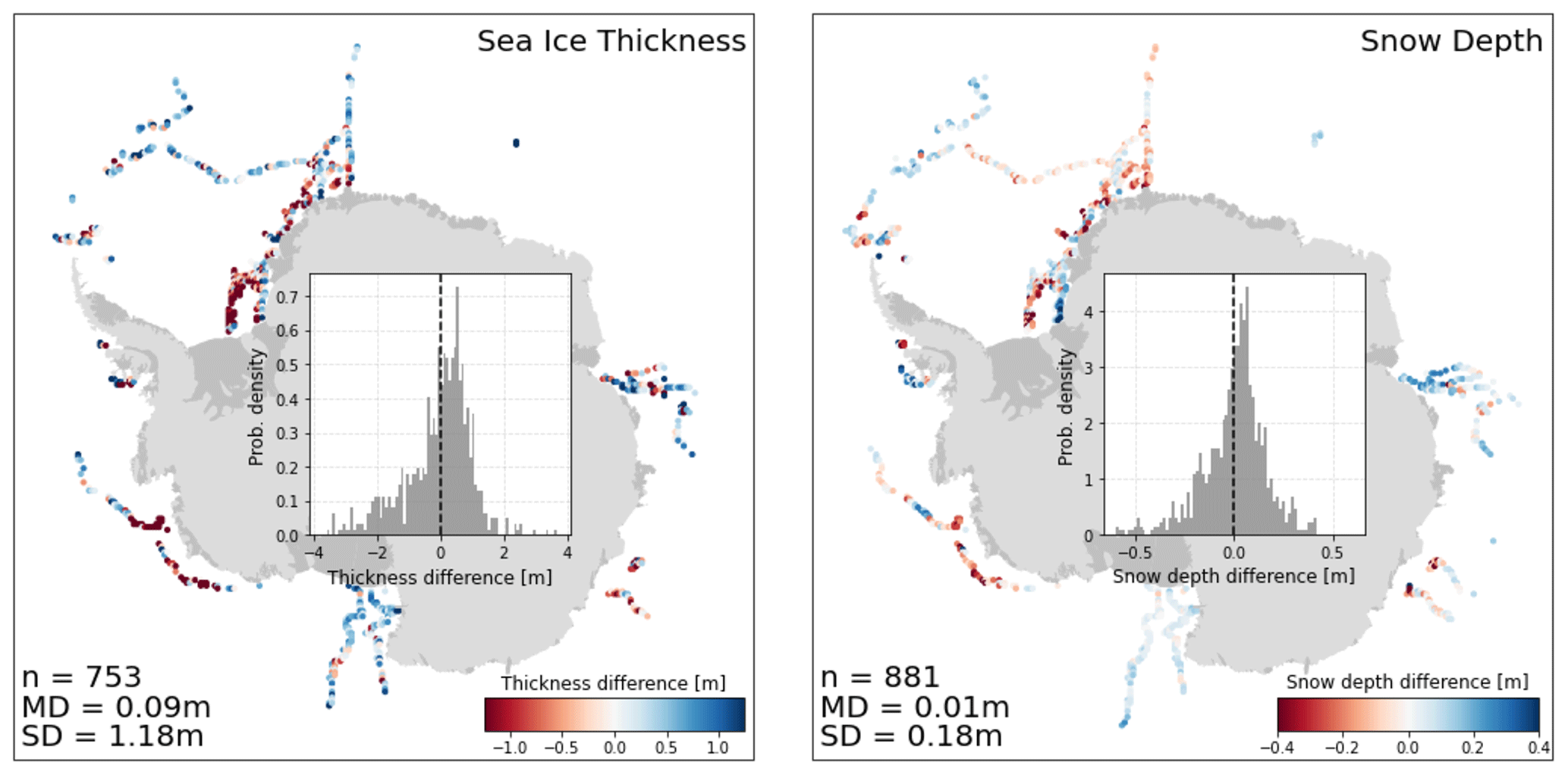
Figure 11 Monthly mean CS2WFA minus the extended ASPeCt data set from Kern (2020), covering the years 2010–2019. Left panel shows sea ice thickness and right panel shows snow depth. Thickness is converted from level ice to total ice thickness using the model in Worby et al. (2008). The inset histograms show the distribution of differences, with the vertical dashed line showing zero mean difference. Bin sizes are 0.1 m for thickness and 0.02 m for snow depth.

Figure 11 (left) shows mean thickness differences of CS2WFA monthly mean sea ice thickness in a given grid cell minus the mean total (level and deformed) ice thickness from the extended ASPeCt data set (Kern, 2020), while the right shows the same for snow depth. Total ice thickness is converted from level ice thickness using the methodology and model in Worby et al. (2008). While the agreement is fairly good overall, there is a clear thin bias of the ship-based data, as seen by the positive mean differences and right-skewed difference distributions. That said, the biases clearly vary between cruise tracks, as some exhibit a negative bias (e.g., in the Weddell Sea) indicating thicker ice estimated by the ship-based observations compared to CS2WFA. Generally, biases in snow depth follow the same sign bias as in thickness for each cruise track. The large standard deviation of differences in thickness estimates highlights how much variation there is around the continent and also underscores reasons that care should be taken when interpreting these results. First, this variation in differences likely arises – at least in part – to the conversion of level ice to total ice thickness, in which the model assumes constant coefficients independent of region. Direct comparisons of only level ice thickness may show better agreement; however, this work is focused on total ice thickness only, and therefore this conversion provides the best estimates available. Additionally, while these ship-based observations are as close as one can come to having pan-Antarctic in situ estimates of thickness, it is important to remember that human eyes are still remote sensing instruments, which are each subject to their own unique biases. For these reasons, it is clear that one must use caution when validating satellite-based thickness estimates to ship-based estimates.

In addition to the ship-based comparisons, this work compares CS2WFA estimates of freeboard, snow depth, and thickness to that from airborne and satellite-based platforms. These comparison measurements bring their own uncertainties and caveats. Most obvious is that these instruments can be completely different, varying in wavelength, footprint, sampling strategy, and more. Even if the exact same ice was sampled at the exact same time (e.g., in Fig. 3), CryoSat-2 would be recording returns that differ to that from ICESat-2 or OIB. That fact alone makes comparisons difficult. However, it gets more complicated; oftentimes, the comparisons do not occur over the same location or at the same time. This is true in comparisons to Kacimi and Kwok (2020), Worby et al. (2008), and Xu et al. (2021) (Figs. 4, 7, and 11 above), which rely on gridding and averaging over longer time periods to compare the distributions of snow depth and thickness. The external data sets each contain their own assumptions, biases, and algorithms that must be acknowledged when comparing results.

With all of these discrepancies and caveats, one may question whether or not these comparisons are worthwhile. Despite their imperfections however, these comparisons do provide useful information that helps to build confidence in the CS2WFA results. Most notably, using multiple thickness products as points of comparison helps to create a pseudo “distribution” of estimates that allow us to get a broad sense of what the sea ice thickness may look like in a given year or region. General agreement with multiple data sets builds confidence that these results are reasonable over large spatial and temporal scales. Additionally, the along-track freeboard comparison to OIB (Fig. 3) as well as comparisons to ICESat-2 in Fons et al. (2021) suggest CS2WFA can perform well over smaller spatial scales too. These multiple comparisons with estimates made using different retrieval techniques and having known biases help to provide bounds on the “actual thickness” of Antarctic sea ice, which is discussed further in the next section.

Overall, these comparisons and data sets are all imperfect, which does add additional uncertainty to the accuracy of these CS2WFA estimates. However, the repeated good agreement across variables and temporal/spatial scales adds confidence that these CS2WFA estimates are within reason. Longer-term, independent validation data sets – similar to the Beaufort Gyre moorings in the Arctic (WHOI, 2018) – would be invaluable to better assess these and future estimates of Antarctic sea ice thickness.

5.2 Toward a reconciled laser–radar altimetry thickness record

With an 11+ year time series of Antarctic sea ice thickness from CS2WFA, one can start connecting the snow freeboard-derived satellite-altimetry-based record of thickness that began with ICESat from 2003–2008 (Kurtz and Markus, 2012) and continues with ICESat-2 (2018–present). Figure 12 shows a full time series with thickness estimates from all three instruments (blue from ICESat, black from CryoSat-2, and green from ICESat-2). Here, we attempt to constrain the “actual” thickness of Antarctic sea ice by highlighting the range in estimates based on the technique used.

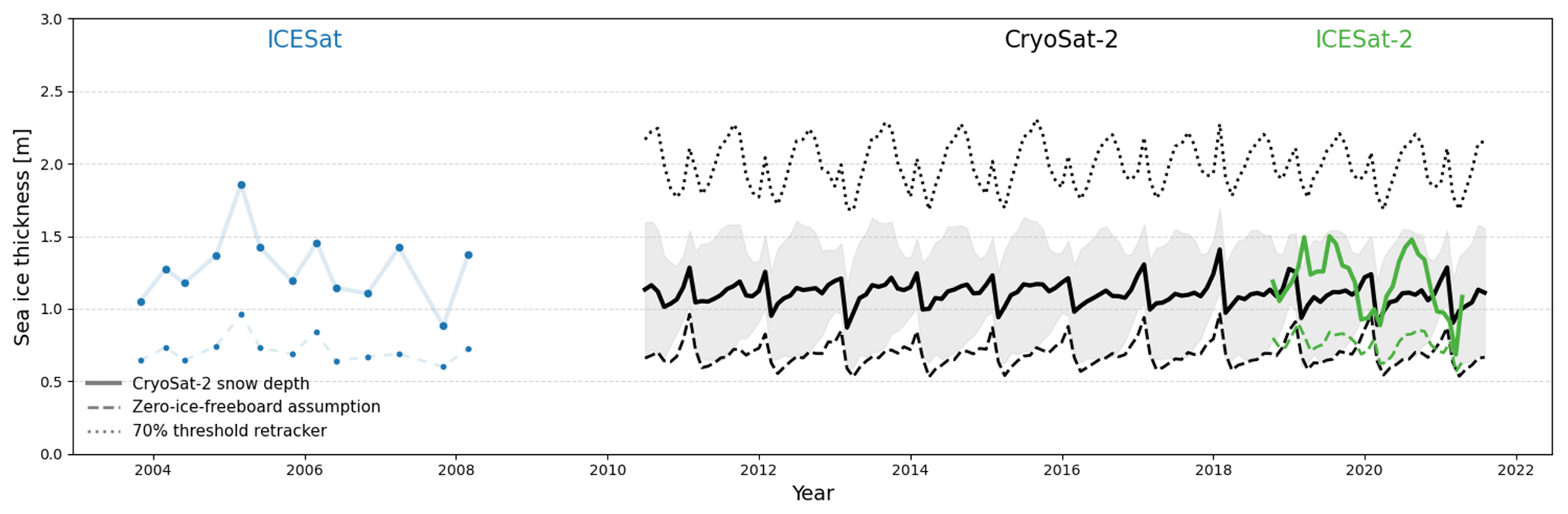
Figure 12 Combined pan-Antarctic sea ice thickness time series from ICESat (Kurtz and Markus, 2012, blue), CryoSat-2 (CS2WFA; black), and ICESat-2 (ATL10; green). Solid lines are sea ice thickness computed with CS2WFA snow depths, while dashed lines are thicknesses computed using the zero-ice-freeboard assumption. The dotted line shows the thickness computed using a 70 % threshold retracking procedure. The shaded region gives the estimated uncertainty in CS2WFA thicknesses. Monthly CryoSat-2 snow depths were used to compute CryoSat-2 and ICESat-2 thicknesses, while an average snow depth climatology was used to compute ICESat thickness. Note that ICESat operated in discrete campaigns, and the faint blue lines shown simply connect these points and do not show the seasonal cycle.

In Fig. 12, the solid lines represent thickness estimates made using the snow depths from CS2WFA and can be thought of as our “best-estimate” thickness for the given period (h_i). For CS2WFA and ICESat-2 thicknesses, the monthly average snow depth grids are used in the calculation, while for ICESat, a monthly snow depth climatology derived from these CS2WFA snow depths are used. Mean values are between ∼ 0.7 and 1.5 m for CryoSat-2 and ICESat-2, while ICESat shows thicknesses between ∼ 0.9 and ∼ 1.8 m on average. The shaded region around the CS2WFA thickness time series represents our estimated thickness uncertainty as calculated in Sect. 3.4. While the solid black line represents the best estimate from CS2WFA, the shaded region provides an upper and lower bound on what we estimate the “actual” thickness to be. It is encouraging that the ICESat-2 thicknesses – despite showing differences from CS2WFA – fall within the range of uncertainty.

The dashed lines in Fig. 12 indicate thicknesses computed using the ZIF assumption (h_i−ZIF). It is clear that using the ZIF assumption results in a thinner ice cover, with mean values always less than 1 m. It is likely that h_i−ZIF is an underestimate of the actual thickness, given that the ZIF assumption is not always valid in all regions and seasons (Kwok and Kacimi, 2018; Kacimi and Kwok, 2020). However, h_i−ZIF follows closely along the lower bound of the CS2WFA uncertainty range, suggesting that it can be considered as a lower constraint on the actual sea ice thickness.

On the contrary, the dotted line in Fig. 12 shows the thickness estimated using a 70 % threshold retracker on the CryoSat-2 data (h_i−70). These values assume the 70 % power level on the CryoSat-2 waveforms gives the snow–ice interface elevation (and thus ice freeboard), estimates the snow depth by subtracting from the waveform-fitting-retrieved air–snow interface elevation, and estimates thickness using this snow depth and freeboard. It is apparent that h_i−70 values are much thicker than other estimates, with mean values around 2 m on average. It is likely that these values are an overestimate of the actual thickness, given what is known about radar penetration into the snow cover over Antarctic sea ice and how 70 % retrackers have been found to overestimate the snow–ice interface elevation (Schwegmann et al., 2016; Paul et al., 2018; Hendricks et al., 2018; Kacimi and Kwok, 2020). An interesting feature in the h_i−70 time series is that the annual maxima occur primarily in the late winter to early spring, differing from the other CryoSat-2 time series but similar to that from ICESat-2. This difference suggests a possibility that the large area of seasonal sea ice in late winter – with very different surface properties than in February – may influence algorithms that assume the dominant return originates from nearer to the air–snow interface, such as the 70 % threshold retracker and laser return, differently than it does the CS2WFA procedure. Additionally, this difference could be related to snow accumulation, which the h_i−70 does not explicitly account for but (as mentioned above) could cause increasing anomalous thickness as snow accumulates. More investigation into the differing impacts of surface type on retrieval methods would be useful to better understand these time series. Overall, the fact that the h_i−70 estimates fall well outside of the CS2WFA uncertainty range suggests that using a simple 70 % threshold retracker alone is not suitable to reliably estimate Antarctic sea ice thickness.

When viewed in this context, some dissimilarities between the thickness estimates and data sources emerge that should be the work of future study. For one, CS2WFA data appear to show small interannual variability, especially in h_i−ZIF, while the ICESat thickness tends to vary more year to year. This is especially apparent in the ICESat h_i, where the range is much larger than is seen in CryoSat-2 and ICESat-2, and could come from the fact that ICESat was operating in discrete “campaigns” and experienced large changes in laser energy over its lifetime. There is a substantial discrepancy in h_i from CS2WFA and ICESat-2 in autumn 2019 and 2020. Given that the snow depths used are identical, these differences arise due to differences in snow freeboard over these months, which was seen in Fons et al. (2021) and thought to be related to the initialization of the CryoSat-2 waveform model. Despite the differences, it is encouraging to see general agreement in the overall mean values of h_i−fs. It is also clear that reliable, independent, and widespread validation data are crucially needed to better uncover the actual thickness distribution from Antarctic sea ice.

It must be noted that the data shown in Fig. 12 are not fully reconciled, and many important points must first be considered before trying to relate these data statistically or with more confidence. For one, the differences in spatial resolution and geometric sampling could have substantial impacts on the freeboard – and therefore the thickness – distributions. This effect was discussed as a potential reason for CryoSat-2–ICESat-2 differences in Fons et al. (2021) but would be further complicated by adding in another sensor (ICESat) with a different footprint size. Also, the frequency differences between radar and laser must be taken into account when assessing the data, as the varying responses from sea ice and heterogeneous surfaces can impact the surface-type classification, which can bias the freeboard retrievals (Tilling et al., 2019) and influence the thickness.

A final difficulty relates to validating measurements and comparing them to each other and to independent data sets. No temporal overlap occurred between ICESat and CryoSat-2, which increases the difficulty in trying to reconcile the measurements. Instead, independent measurements must be used that exist for both platforms. While these independent measurements spanning the ICESat and CryoSat-2 operation exist in the Arctic (e.g., the WHOI Beaufort Gyre moorings, WHOI, 2018), they do not currently exist for Antarctic sea ice. At the time of this writing, CryoSat-2 and ICESat-2 are in coincident operation with the CryoSat-2 orbit optimized for more frequent overlaps with ICESat-2 in the Southern Hemisphere. These CRYO2ICE data (European Space Agency, 2018) will be especially useful in reconciling and extending the sea ice thickness record.

6 Conclusions

In this work, estimates of Antarctic snow freeboard, snow depth on sea ice, and sea ice thickness derived from CryoSat-2 have been shown. The physical model and waveform-fitting process introduced in Fons and Kurtz (2019) and improved in Fons et al. (2021) was applied to all CryoSat-2 data over the Southern Ocean between July 2010 and August 2021, and results were aggregated into monthly and seasonal averages.

Snow freeboard estimates from CS2WFA showed a comparable along-track profile to that from OIB, with mean differences under 4 cm. Pan-Antarctic monthly averaged snow depths for the year 2019 derived from this method showed a high bias when compared to that from KK20, ranging between 0.2 to 7.5 cm. Seasonal means from the entire CryoSat-2 period range from 16 cm in autumn to 25 cm in summer.

The retrieved freeboard and snow depth data were then combined to estimate sea ice thickness. Spatial patterns appeared as expected (similar to that from KK20, Kurtz and Markus, 2012, and others) and had climatological monthly mean values over the CryoSat-2 period ranging between 0.95 and 1.26 m. These values are potentially on the thick side, especially compared to estimates from Worby et al. (2008), as one would expect thinner ice during certain months of new ice growth. However, the retrieved thicknesses tend to agree with other satellite-based estimates, specifically those from Xu et al. (2021) and KK20. A time series from 2010 to 2021 was constructed that shows some interannual variability but highlights a consistent seasonal cycle and range of values.

Intra-decadal changes in sea ice thickness and volume over this CryoSat-2 period were explored, showing competing negative (thinning) and positive (thickening) regional trends between 2010–2021. These competing changes resulted in a slight (less than 0.5 cm) net pan-Antarctic thinning in all seasons expect for summer, which shows a slight thickening over this time range. The relatively short time period of 11 years simply provides a snapshot of changes and precludes any indication of substantive trends in sea ice thickness, especially given the decadal-scale oscillations that can drive changes in the sea ice cover.

Overall, this work has shown a decade-plus-long time series of Antarctic sea ice thickness from CryoSat-2 using snow depths and snow freeboards retrieved from the CS2WFA method, complementing the snow freeboard-derived Antarctic sea ice thickness record that began with ICESat (Kurtz and Markus, 2012) and continues with ICESat-2 (Kacimi and Kwok, 2020; Xu et al., 2021). It is clear that more independent validation measurements are required to better get a sense of the “true value” of Antarctic sea ice and snow thickness, which would help in combining estimates from these three instruments into a cohesive time series. Additionally, future work is necessary to establish biases between the instruments and reconcile thickness estimates in light of the geometric sampling and frequency-related discrepancies. The current temporal overlap between CryoSat-2 and ICESat-2 observations is invaluable for comparison and validation and is even more beneficial now that the CRYO2ICE campaign has been optimized for the Southern Hemisphere (European Space Agency, 2018). Reconciling these observations will lead to a better understanding of recent changes in Antarctic sea ice thickness.