the Creative Commons Attribution 4.0 License.
the Creative Commons Attribution 4.0 License.
 | 21 Jun 2023
Exploring the use of multi-source high-resolution satellite data for snow water equivalent reconstruction over mountainous catchments
Valentina Premier
Carlo Marin
Giacomo Bertoldi
Riccardo Barella
Claudia Notarnicola
Lorenzo Bruzzone
The hydrological cycle is strongly influenced by the accumulation and melting of seasonal snow. For this reason, mountains are often claimed to be the “water towers” of the world. In this context, a key variable is the snow water equivalent (SWE). However, the complex processes of snow accumulation, redistribution, and ablation make its quantification and prediction very challenging. In this work, we explore the use of multi-source data to reconstruct SWE at a high spatial resolution (HR) of 25 m. To this purpose, we propose a novel approach based on (i) in situ snow depth or SWE observations, temperature data and synthetic aperture radar (SAR) images to determine the pixel state, i.e., whether it is undergoing an SWE increase (accumulation) or decrease (ablation), (ii) a daily HR time series of snow cover area (SCA) maps derived by high- and low-resolution multispectral optical satellite images to define the days of snow presence, and (iii) a degree-day model driven by in situ temperature to determine the potential melting. Given the typical high spatial heterogeneity of snow in mountainous areas, the use of HR images represents an important novelty that allows us to sample its distribution more adequately, thus resulting in highly detailed spatialized information. The proposed SWE reconstruction approach also foresees a novel SCA time series regularization technique that models impossible transitions based on the pixel state, i.e., the erroneous change in the pixel class from snow to snow-free when it is expected to be in accumulation or equilibrium and, vice versa, from snow-free to snow when it is expected to be in ablation or equilibrium. Furthermore, it reconstructs the SWE for the entire hydrological season, including late snowfall. The approach does not require spatialized precipitation information as input, which is usually affected by uncertainty. The method provided good results in two different test catchments: the South Fork of the San Joaquin River, California, and the Schnals catchment, Italy. It obtained good agreement when evaluated against HR spatialized reference maps (showing an average bias of −22 mm, a root mean square error – RMSE – of 212 mm, and a correlation of 0.74), against a daily dataset at coarser resolution (showing an average bias of −44 mm, an RMSE of 127 mm, and a correlation of 0.66), and against manual measurements (showing an average bias of −5 mm, an RMSE of 191 mm, and a correlation of 0.35). The main sources of error are discussed to provide insights into the main advantages and disadvantages of the method that may be of interest for several hydrological and ecological applications.
- Article
(5704 KB) - Full-text XML
-
Supplement
(4127 KB) - BibTeX
- EndNote


Seasonal snow accumulation and melt are crucial for the hydrological cycle and the total water supply. Mountains are claimed to be the “water towers” of the world given the large impact of snow on local and global water resources (Immerzeel et al., 2020). The contribution of snow-dominated catchments to streamflow ranges from 40 % of total flow to sometimes more than 95 %, depending on the region (Viviroli et al., 2003). Therefore, it is essential to estimate the amount of water stored during winter to forecast river discharge and to correctly plan human activities such as agriculture irrigation, drinking water supply, and hydropower production (DeWalle and Rango, 2008; Beniston et al., 2018). In mountain regions, the snow distribution is highly variable in space and time due to redistribution processes (Balk and Elder, 2000), thus limiting the effectiveness of available in situ measurements. Especially in remote areas, continuous and spatialized observations are rare (Rees, 2005). Hence, remote sensing (RS) represents a valuable tool for snow hydrology.
A correct spatial characterization of snow properties requires both knowledge about the extent of the snow cover, i.e., the snow cover area (SCA), and appropriate snowpack information. A key variable is the snow water equivalent (SWE), i.e., the total amount of water stored in the snowpack released upon complete melting. Although a long list of SCA detection methods that exploit multispectral optical satellites is available in the literature (e.g., Dietz et al., 2012; Dong, 2018), we do not have operational methods to directly map SWE with high spatial resolution (HR). Direct SWE observations are limited to point measurements by manual sampling, snow scales, and/or snow pillows (Archer and Stewart, 1995; Meløysund et al., 2007) or have a limited spatial footprint (∼500 m) such as cosmic-ray neutron probes (Schattan et al., 2019). Spatialized snow depth (SD) information can be provided by differential lidar altimetry (Painter et al., 2016) or stereo photogrammetry (Deschamps-Berger et al., 2020). However, these methods can be applied only to limited areas and with a low temporal sampling. Moreover, the derivation of SWE from SD requires additional a priori information to infer the snow density (Helfricht et al., 2018). Physically based snow models represent a valid alternative (e.g., Lehning et al., 2006; Vionnet et al., 2012; Endrizzi et al., 2014) that can provide HR SWE information for large areas. Nonetheless, their accuracy is strongly limited by the uncertainty in the input data (Engel et al., 2017; Günther et al., 2019) and by the gravitational and wind-induced snow redistribution processes (Jost et al., 2007; Mott et al., 2018). One of the main challenges is to obtain an accurate precipitation field given the strong spatial variability of the variable related to orography, a generally scarce sampling density of the phenomenon that strongly influences the interpolation results, and possible inaccuracies in the measurements caused, for example, by undercatching (e.g., Prein and Gobiet, 2017).
Passive and active microwave sensors can potentially provide information about the snowpack. In particular, the first ones are used to retrieve long time series of SWE by exploiting the correlation between brightness temperature and SWE (Pulliainen et al., 2020). However, the observations are limited by a spatial resolution of 25 km and are not suitable for mountain regions. Active microwave sensors, such as synthetic aperture radars (SARs), were investigated for HR retrieval of SWE (Ulaby et al., 1981; Shi et al., 1994; Baghdadi et al., 1997; Rott et al., 2010) and differential SWE (Guneriussen et al., 2001; Leinss et al., 2015). Despite the better spatial resolution, active microwave sensors suffer from the complexity of nonlinear effects introduced in the total backscattering, such as snow layering, surface roughness, snow density, and grain type and size, which in turn are all affected by the complex snow metamorphism and change in time. Furthermore, all of these techniques work only in dry snow conditions, whereas the scarce penetration of the electromagnetic signal in wet conditions invalidates their applicability to monitor the evolution of the SWE during the melting season. For more details on SWE retrieval using SAR acquisitions, several review articles are available (e.g., Tsang et al., 2022).
Despite recent developments, SAR is still far from providing unambiguous information on SWE in all conditions. However, it represents a promising tool to monitor the melting phases of the snowpack, i.e., the moistening, ripening, and runoff phases or, in other words, the presence and evolution of liquid water inside the snowpack (Marin et al., 2020). If the snow regime presents distinct ablation and accumulation periods, the onset of runoff (i.e., when the SWE reaches its maximum) derived by SAR adds value to the snow depletion curve (SDC) when combined with optical data. The SDC is a function that describes the relationship between SCA and SD or SWE (Cline et al., 1998). Thus, time series of SCA can be used to provide an indirect measurement of SWE (Yang et al., 2022). SWE is a function of the duration of the snow cover, which intrinsically considers the energy exchanges responsible for the melting process (Durand et al., 2008). For example, shallow snowpacks and high melt rates are associated with an SDC having a high derivative, while deep snowpacks and low melt rates are characterized by a longer curve (e.g., Pimentel et al., 2015, 2017). Consequently, spatial accumulation and ablation variabilities, which are related to the topography of the study area (Anderton et al., 2002), result in different persistence of the snowpack (Luce et al., 1998). Therefore, knowing the SDC and the SWE maximum at the end of the accumulation for a catchment allows deriving the evolution of SWE during melting. This intuitive idea opens the possibility of assimilating SCA and SDC information into physically based snow models to correct SWE evolution and improve simulations (Arsenault and Houser, 2018).
Similarly, SDC can be exploited in combination with distributed snowmelt models to reconstruct SWE time series in reanalysis (Martinec and Rango, 1981; Molotch and Margulis, 2008; Rittger et al., 2016). Unlike the methods that require known precipitation and meteorological forces to redistribute the snowpack during the accumulation, SWE reconstruction builds the SWE time series backward from the last day of snow presence. To this purpose, these approaches exploit the estimation of the potential melt energy and the knowledge about the presence of snow cover, thus simplifying the solution of the problem. The SWE reconstruction approaches showed good performances over large basins and even mountain ranges (Bair et al., 2016). Nevertheless, the accuracy of the results depends on a robust estimation of both the potential melting and SCA. For the first one, several methods were proposed that range from a simple yet robust degree-day (DD) model (Martinec and Rango, 1981) to a complete radiation energy computation that also takes into account the snow albedo (Bair et al., 2016). To estimate SCA, many works presented in the literature exploit low-resolution (LR) multispectral satellite images, since their large swath allows a high repetition time, i.e., with a daily or sub-daily acquisition. This mitigates cloud obstruction issues and involves a proper SCA sampling. However, LR images do not provide sufficient spatial detail on the variability of the snow cover evolution in the mountains, which is on the order of a few dozen meters. Moreover, the use of LR images results in a nonlinear combination of the different contributions of the elements within the pixel, and this may induce large errors in the snow classification approaches, especially in complex terrains. On the other hand, the use of HR snow maps introduces important benefits in both determining SWE and forecasting streamflow (Molotch and Margulis, 2008; Li et al., 2019). Landsat products were used to retrieve SCA in many papers in the literature (e.g., Molotch et al., 2004; Molotch and Bales, 2005, 2006). However, a Landsat satellite acquires an image every 16 d (at the Equator). With the introduction of the Copernicus Sentinel-2 (S2) mission, HR images are made available with an improved temporal resolution of 5 d (at the Equator). This opens up new opportunities to monitor heterogeneous snow conditions in the mountains. Unfortunately, due to cloud coverage, useful acquisitions are reduced by 50 % in the Alps (Parajka and Blöschl, 2006). Therefore, even if the Landsat images are exploited together with the S2 images, only a few acquisitions are available per month. Recently, we proposed an approach to the reconstruction of daily HR snow cover maps. The approach performs a gap-filling and a downscaling of the snow cover fraction (SCF) maps derived at LR based on the idea that the melting and accumulation patterns repeat interannually (Premier et al., 2021; Revuelto et al., 2021). Therefore, by observing partial HR or LR acquisitions it is possible to reconstruct a daily HR snow cover.
This work explores the use of multi-source satellite data to reconstruct HR daily SWE time series at a spatial resolution of 25 m. To achieve such detail, we propose as main novelties the use of a daily HR SCA time series together with accurate information on the melting phase from SAR data. To this purpose, we also introduce the concept of the snow state of a pixel, which represents the direction of the change in SWE for that pixel: that is, accumulation (SWE increase), ablation (SWE decrease), or equilibrium (constant SWE). This allows reconstructing SWE without the need for spatialized precipitation data. Indeed, the method redistributes the amount of melting by exploiting the information about the state rather than quantifying the precipitation input. Moreover, the state allows us to set up a novel regularization of the SCA time series. In the paper, we also present a critical analysis of the main sources of error to provide insights into the main advantages and disadvantages of the method that may be of great interest for several hydrological and ecological applications. We explore the applicability of the method to two mountainous catchments: (i) the South Fork of the San Joaquin River (SFSJR), located in the Sierra Nevada – California (USA), and (ii) the Schnals catchment, located in the Alps – South Tyrol (Italy).
The paper is structured into five sections. Section 2 presents the different steps of the proposed approach to reconstruct the daily HR SWE. The two test sites considered for experimental validation and the related dataset are presented in Sect. 3. The results obtained are illustrated in Sect. 4. In Sect. 5, we discuss the main sources of errors of the method and the novel SCA regularization. Finally, Sect. 6 draws the conclusions of the work and gives indications for further exploitation of the proposed approach.
The presented approach is made up of three main parts: (i) identification of the state, (ii) characterization of the snow season from the regularized SCA time series, and (iii) calculation of the SWE. The details will be illustrated in the following three subsections. As depicted in Fig. 1, the method starts with the identification of the state, i.e., accumulation, ablation or equilibrium (see Sect. 2.1). The state information is used first in this step to both regularize the SCA time series taking into account impossible transitions and correctly determine the beginning and end of the season (see Sect. 2.2). With impossible transitions, we indicate an erroneous change in the pixel class from snow to snow-free when the state is accumulation or equilibrium and, vice versa, the change from snow-free to snow when the state is ablation or equilibrium. The regularized time series of SCA is then used with the potential melting to reconstruct the daily HR SWE maps (see Sect. 2.3). The state information is used again in this step (i) to redistribute the total amount of SWE calculated for the melting in the accumulation period and (ii) to include late snowfall that occurs after the peak of accumulation in the reconstruction. Both cases are generally omitted in state-of-the-art SWE reconstruction methods (e.g., Martinec and Rango, 1981; Molotch and Margulis, 2008).
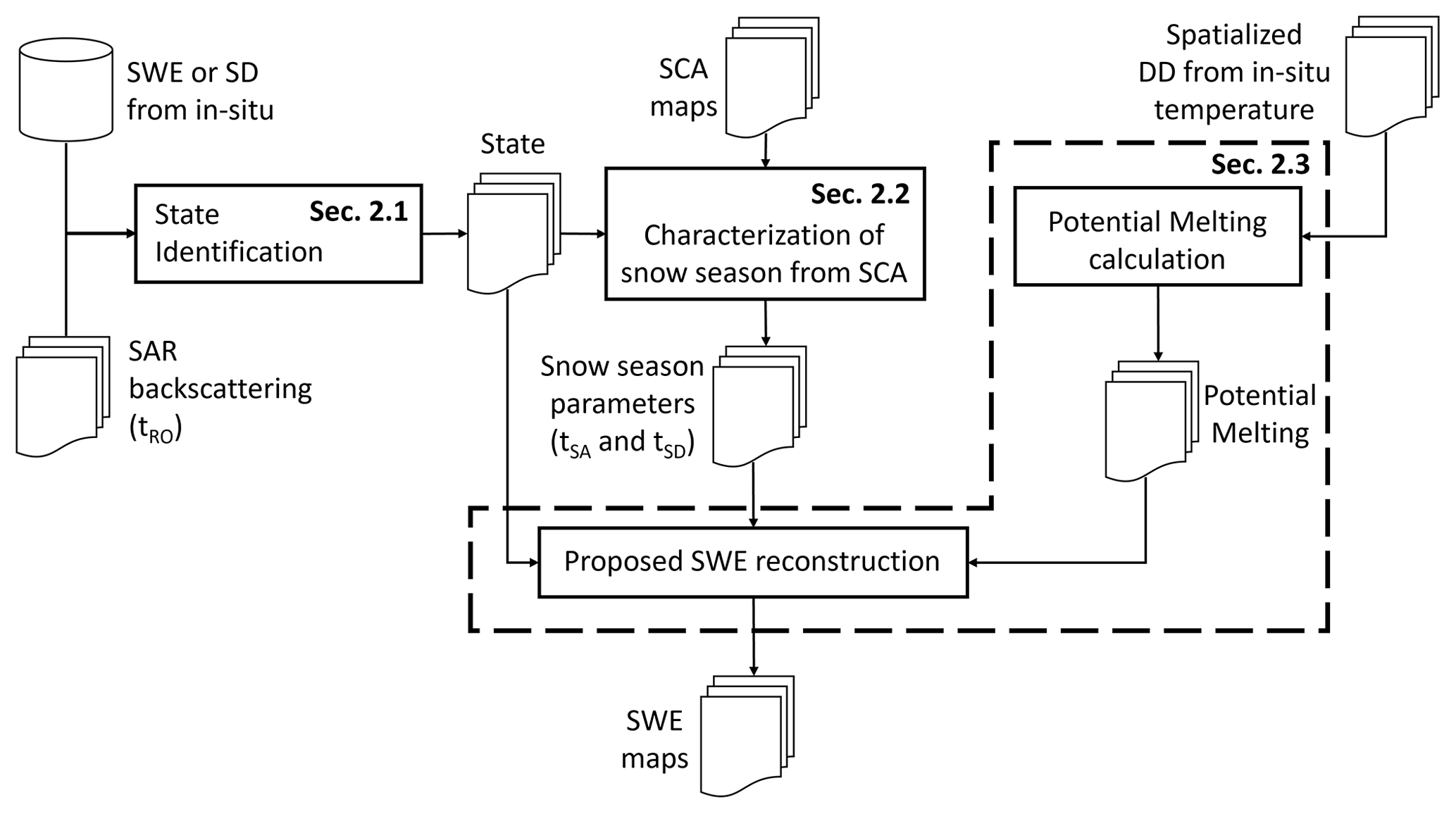
Figure 1Workflow of the proposed approach showing the three main steps: (i) state identification, (ii) characterization of snow season from SCA, and (iii) SWE reconstruction. The inputs are (i) SWE or SD from automatic weather stations (AWSs), (ii) SAR backscattering time series, (iii) a daily HR SCA time series, and (iv) daily spatialized potential melting maps derived from AWSs. As output, we obtain the daily HR SWE maps.
2.1 Identification of the state
Three states are introduced to describe possible SWE changes within a pixel, i.e., ΔSWE between two times t−1 and t. As illustrated in Table 1, the states are (i) accumulation, which represents an increase in SWE (ΔSWE>0), (ii) ablation, which represents a reduction in SWE (ΔSWE<0), and (iii) equilibrium, which represents a stable SWE (ΔSWE=0).
Table 1Definition of the three possible states: accumulation, ablation, and equilibrium. The possible class transitions at pixel level associated with the state are described.
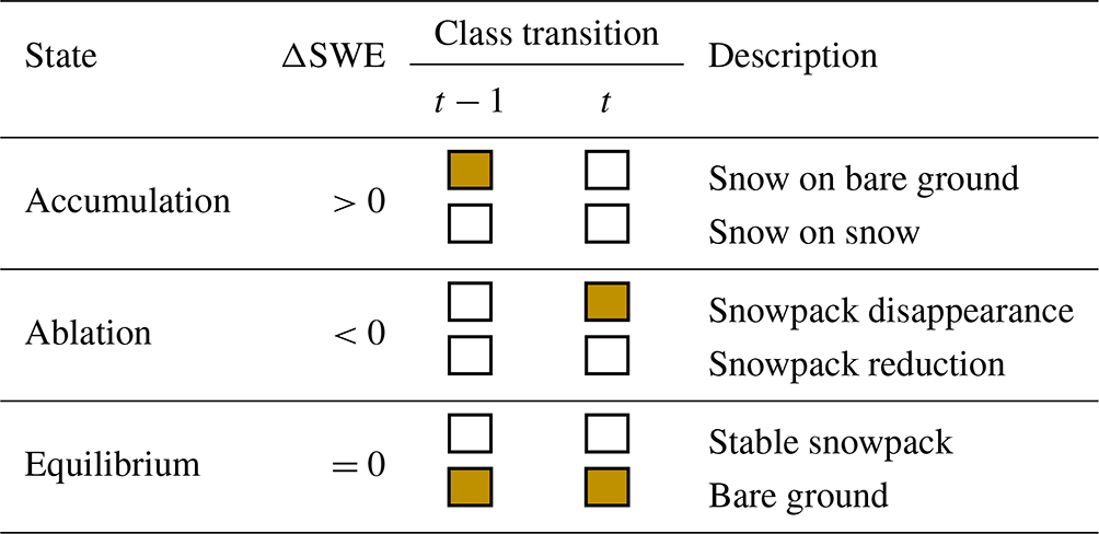
Legend: ![]() = snow
= snow ![]() = snow-free
= snow-free
There are several phenomena that cause an SWE variation, such as snowfall, melting, sublimation, human activities, and redistribution due to wind or gravitational transport, e.g., avalanches. However, we refer mainly to snowfall if in accumulation and to melting if in ablation. Indeed, we propose estimating the SWE to be added to the reconstruction by considering a quantity proportional to the snow depth or SWE daily increment. Thus, in an ideal case, we include only fresh snow as the main driver. Similarly, the amount of SWE to be subtracted is calculated using a DD model, and therefore it only represents melting. Trivially, SWE remains constant when in equilibrium. Note that the state is defined on a daily scale, which corresponds to the temporal resolution of the exploited HR SCA time series. In this work, the diurnal fluctuations in meteorological forces are not considered.
The state varies pixel-wise due to the topography and meteorology of the study area. However, it is difficult to extrapolate this information with the necessary spatial detail. In the following paragraphs, we propose simplified strategies for the accumulation and ablation determination. If none of them are identified, the state is equilibrium.
2.1.1 Accumulation identification
The accumulation identification can be retrieved from a network of automatic weather stations (AWSs) that provide continuous information about the occurrence and elevation of snowfall events: for example, direct SWE measurements or indirect precipitation and SD measurements. Continuous SWE measurements are unfortunately scarcely available. By means of pluviometers and temperature observations, it is possible to split precipitation between liquid and solid and identify the state accordingly. However, these stations are rarely installed at high elevations. SD sensors are more suitable for our purpose, but their observations are often affected by wind and gravitational transport, leading to deposition or removal that can be falsely interpreted as accumulation or ablation. Hence, even if the AWSs are generally situated in locations undisturbed by wind action, it is more convenient to dispose of a large number of AWSs that need to be filtered to exclude possible sensor errors or wind and/or gravitational redistribution. In fact, a station is usually representative of a limited area whose extension is highly variable depending on the complexity of the terrain. In the case of a well-monitored area with stations distributed with elevation, it is possible to divide the catchment into different elevation belts where the snowfall events can be considered nearly homogeneous. However, in many basins, this might be far from reality. As a common configuration for snow monitoring, we have a single station located at a high point of the catchment, which is informative enough to identify the accumulation events but not their extent. Furthermore, it has been shown in the literature that estimating the snowfall limit can be very challenging (e.g., Fehlmann et al., 2018).
Therefore, the method can be adapted based on the availability of in situ observations. In this study, we made use of SWE and snow depth measurements, since they were available in our analyzed basins. To consider snowfall to be occurring, the increase in SWE or SD should be greater than a certain threshold SDmin/SWEmin that is fixed at 2 cm for SD according to the values found in the literature (Engel et al., 2017), resulting in a value of 2 mm for SWE when considering the typical density of fresh snow (100 kg m−3). Unfortunately, the basins are poorly monitored in terms of these variables, and consequently the snowfall limit cannot be estimated in an appropriate manner. Hence, we consider snowfall to be occurring throughout the snow-covered area of the catchment. We acknowledge that this assumption may result in less accurate SWE estimation, especially in the case of mixed states. For example, snowfall can be observed at high elevations, together with rain on snow at low elevations, causing snowmelt. However, we assume that the effect of these events on the total SWE balance is small enough to be considered negligible, as we will discuss in Sect. 5.2.
In summary, when the AWSs show an increment greater than a defined threshold, we identify the state as accumulation.
2.1.2 Ablation identification
The ablation can be identified by using a snowmelt model. We consider the simple temperature index model here, which is an empirical model that makes use of air temperature as a proxy for the melting (Ohmura, 2001). When the temperature exceeds a fixed threshold, we expect the pixel to melt. However, this is a simplified approach that does not consider all the components that contribute to snowmelt. More complex formulations include estimates of radiation, sensible heat, latent heat, and ground heat fluxes (e.g., Ismail et al., 2023). Moreover, temperature observations may be sparse, thus affecting the accuracy of the spatialization.
Multi-temporal SAR observations derived from Sentinel-1 (S1) can detect the presence of a melting snowpack, as explained by Marin et al. (2020). The authors investigated the relationship between the SAR backscattering and the three melting phases, i.e., the moistening, ripening, and runoff phase. In detail, they showed that if the SAR backscattering presents a decrease of at least 2 dB, the snowpack gets moistened (Nagler and Rott, 2000). Initially, at the beginning of the moistening phase this decrease affects only the afternoon measurements. When it also affects the morning measurements, the ripening phase starts. Finally, the backscattering increases as soon as the SWE starts to decrease, which corresponds to the beginning of the runoff phase. This moment represents the first contribution of the snowpack to the release of water. Empirical experiments at five selected test sites showed that the melting phases were identified with an RMSE of 6 d for the moistening phase, 4 d for the ripening phase, and 7 d for the runoff phase.
The multi-temporal analysis of the SAR backscattering represents a novel way to identify ongoing melting in a spatialized manner. The runoff onset (tRO) represents the time when the snowpack is isothermal. In this way, information about the cold content of the snowpack is incorporated into the DD model excluding incorrect early melting. However, the methodology presented by Marin et al. (2020) may fail in areas such as forests. As shown by Darychuk et al. (2023), the characteristic “U-shaped” signature of the backscattering signal is less evident in mature forest, also depending on canopy structure, composition, and density. The signal can be noisier due to the scattered contribution by the canopy. Hence, we propose applying the method only for pixels that present clear U-shaped backscattering, which can be also present for forested areas. To this purpose, we apply a multi-temporal analysis to the different available S-1 tracks. First, we identify if a drop of at least 2 dB is present in the time series. Second, the minimum is selected after this drop. When more tracks are available, we set the first minimum as the beginning of the runoff. Therefore, we propose considering a pixel to be in ablation for the entire period ranging from the backscattering minimum to the disappearance of the snow cover identified by optically derived time series. For the pixels that do not present the characteristic U shape, we rely on the DD model for the identification of the melting state.
In summary, we propose identifying the state of ablation for a specific date and a single pixel if the following conditions are met: (i) there is no accumulation on the date in question, and (ii) the SAR backscattering shows an increase after a relevant drop of at least 2 dB, indicating that the minimum value corresponding to tRO has been reached, and (iii) the degree day (as shown in Eq. 2) is greater than 0.
2.2 Characterization of the snow season from regularized SCA time series
A necessary input for the proposed SWE retrieval is a daily HR SCA time series or, in other words, the date of snow appearance tSA and disappearance tSD. As mentioned in the Introduction, such a product is not available directly from remotely sensed images due to limitations in the revisit time and cloud obstruction. Therefore, it is necessary to reconstruct it. Among the various methods present in the literature, we use the approach proposed by Premier et al. (2021), which merges information coming from a sparse long HR time series and a continuous daily LR time series acquired in the period of interest. Gap-filling and downscaling steps are performed by applying a set of hierarchical rules based on historical analyses and topographical features. The main idea behind the approach is that snow patterns persist over time and follow a regular distribution that is strongly dependent on the topography and meteorology of the area of interest (Mendoza et al., 2020). We refer the reader to Premier et al. (2021) for details.
Despite the generally accurate results of the abovementioned approach (the overall accuracy is empirically estimated to be around 92 %), the HR SCA output is still affected by possible inconsistencies. Errors may arise either from the classification algorithm applied to the multispectral input images or from the reconstruction approach. In detail, we can highlight the presence of two main sources of errors: (i) an underestimation of snow presence in forested areas when the snow falls below the canopy and is thus not visible from the satellite point of view (i.e., snow on the ground) and (ii) the missed identification of snow patches at the end of the season. The first error source is due to the fact that the classification methods used for snow retrieval for both HR and LR images rely only on the spectral information measured inside the resolution cell of the sensor without a dedicated module for inferring the presence of snow when hidden by the canopy. This affects the detection of snow on the ground, particularly for HR images, since the low-resolution cell is likely to contain a majority fraction of the canopy, especially over very dense forests. This problem is instead mitigated for LR pixels that are likely to contain not only forested areas but also open fields where the snow is visible, increasing in this way the possibility of detecting the snow presence. Therefore, it is possible to observe local decreases in SCA mainly in correspondence with an HR acquisition. The second error involves mostly LR images whose spatial detail is not enough to detect mixed pixels with low SCF. This is an error that persists over time since LR acquisitions are more frequent than HR acquisitions, while a local increase in SCA is shown in correspondence with an HR acquisition.
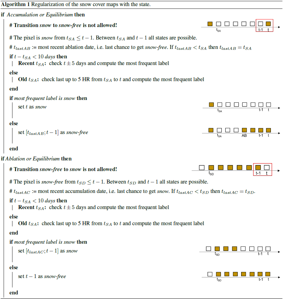
The state concept introduced in Sect. 2.1 can be used to regularize the SCA. According to Table 1, only transitions of the pixel class that are coherent with the state are allowed. When in accumulation the pixel can only turn from snow-free to snow if snow falls on bare ground, or it can continue to be snow if snow falls on already deposited snow. Similarly, when in ablation the pixel can only turn from snow to snow-free if the snow cover disappears, or it can remain snow if the snow cover partially melts. Finally, when in equilibrium the pixel continues to be snow or snow-free depending on the situation. Therefore, we can define the impossible transitions: (i) a pixel cannot turn from snow to snow-free from t−1 to t if in accumulation or equilibrium, and (ii) a pixel cannot turn from snow-free to snow from t−1 to t if in ablation or equilibrium.
When facing a wrong transition, we do not know a priori whether the correct label is the one at t−1 or the one at t. To derive the correct interpretation, we consider an appropriate time window and compute the most frequent label according to the majority rule. The time window is chosen differently in the case in which we are facing a recent or an old date of snow appearance tSA. In detail, for a given pixel, we consider the following.
-
A recent date of snow appearance when d. In this period, we often observe missed detection of snow under the canopy, especially by HR sensors. Under this condition, we do not expect fast changes, since the temperatures are likely to be low, and thus the potential melting is low (see Eq. 1). Consequently, we propose considering a daily time window of ±5 d from t to check what is the most persistent label of the considered pixel (Parajka and Blöschl, 2006).
-
An old date of snow appearance when d. If the final melting has already started, changes may be quick, and the most common situation is the missed detection of mixed pixels as snow patches. We observe that in this period HR sensors detect snow patches that are completely omitted by LR sensors. In this case (i) the dates after t are not informative since the snow patches disappear quickly, and (ii) daily SCA may not be informative when derived from LR. For this reason, we consider only the last up to five dates when an HR was originally acquired in a time window between tSA and t.
Once we determine the state and whether we are handling a recent or old tSA, we can compute the most frequent label in the considered time window and apply the following correction (see Algorithm 1). The correction is performed by advancing forward in time; i.e., we assume that the previous labels are always coherent with the previous states. If we are in accumulation or equilibrium, a transition from snow to snow-free is not allowed. If the pixel is labeled snow in t−1, then it means that, for the sake of coherence, it turned into snow in tSA. We also know the date of the most recent ablation tlastAB, i.e., the last chance that the pixel had to become snow-free. Therefore, we compute the most frequent label accordingly with the majority rule described in the previous paragraph, which varies depending on whether the snowfall is old or recent. If (i) the most frequent label is snow, t is replaced with snow; (ii) if the most frequent label is snow-free, all times starting from tlastAB (or tSA, tlastAB<tSA) up to t−1 are replaced with snow-free.
Analogously, the transition from snow-free to snow is not allowed in ablation or equilibrium. If the pixel is labeled as snow-free at t−1, it means that, for the sake of coherence, it turned to snow-free at tSD. We also know the date of the most recent accumulation tlastAC, i.e., the last chance that the pixel had to become snow. Hence, we compute the most frequent label accordingly with the majority rule, and if it results in (i) the most frequent label being snow-free, t is replaced with snow-free; (ii) if the most frequent label is snow, all times starting from tlastAC (or tSD, tlastAC<tSD) up to t−1 are replaced with snow.
2.3 HR SWE reconstruction
Once the state is defined as described in Sect. 2.1 and the daily HR SCA time series is regularized coherently with the state as described in Sect. 2.2, we can apply the proposed approach to HR SWE reconstruction. As illustrated in Fig. 2, this operation requires calculating the total amount of melting and redistributing it during the snow season according to the preservation of mass and the state. To this purpose, we estimate the daily potential melting with the DD model. For a generic time interval , the potential melting is estimated through the following equation:
where a is the so-called DD factor and varies depending on the area and the snow period. Note that potential melting is considered only after the runoff onset as detected by S1 data. We used a value of a=4.5 mm ∘C−1 d−1 for the SFSJR and a=5.2 mm ∘C−1 d−1 for the Schnals catchment. The coefficient is calibrated by considering the measured SWE and temperature at the AWSs (if available) and also taking into account the range of values derived in previous literature (Hock, 2003). is the DD given by the cumulative sum of the hourly temperatures exceeding a certain threshold:
The threshold temperature is set to 0 ∘C.
The DD is first calculated for each station and then spatially interpolated using a three-dimensional universal kriging routine with linear variogram and elevation as external drift (Murphy et al., 2020). The choice arises from the results of a leave-one-out (LOO) cross-validation (see Sect. S2 in the Supplement). The variogram parameters are automatically calculated at each time step using a “soft” L1 norm minimization scheme. The number of averaging bins is set to six (default value). The kriging is performed on the daily DD values instead of on the raw hourly temperature values to reduce computational times.
We can determine the total amount of melting Mtot by summing all daily for all those days in ablation within the time range [tSA;tSD]. It is worth noting that a single pixel may have more than one snow period, and hence we can have more than a couple of tSA–tSD values. Mtot, which has to be equal to the total accumulation Atot, is then calculated as follows:
Consequently, it is possible to reallocate the total accumulation on days that are in accumulation:
where is a coefficient that represents the amount of snowfall. If we have a network made by S AWSs with measured SWE (or similarly, SD), k is set proportional to the observed snowfall:
Note that the number of days in accumulation varies for each pixel, and consequently, the coefficient is a function of time and space. Thus, it is possible to determine the final output, i.e., a daily HR SWE time series, by applying the following rules pixel-wise.
It may happen that during ablation temperatures are low and the term is equal to 0, thus coinciding with the equilibrium state.
It is worth stressing the fact that although sublimation, redistribution, and gravitational transport are not explicitly taken into account in Eq. (6), their consequences are implicitly observed as a longer persistence of snow on the ground that is detectable through the use of an accurate SCA time series. Moreover, by providing an approximation of the accumulation events, we also consider late snowfall that can occur during the main melting season and that is a major source of error in state-of-the-art methods (Slater et al., 2013a).
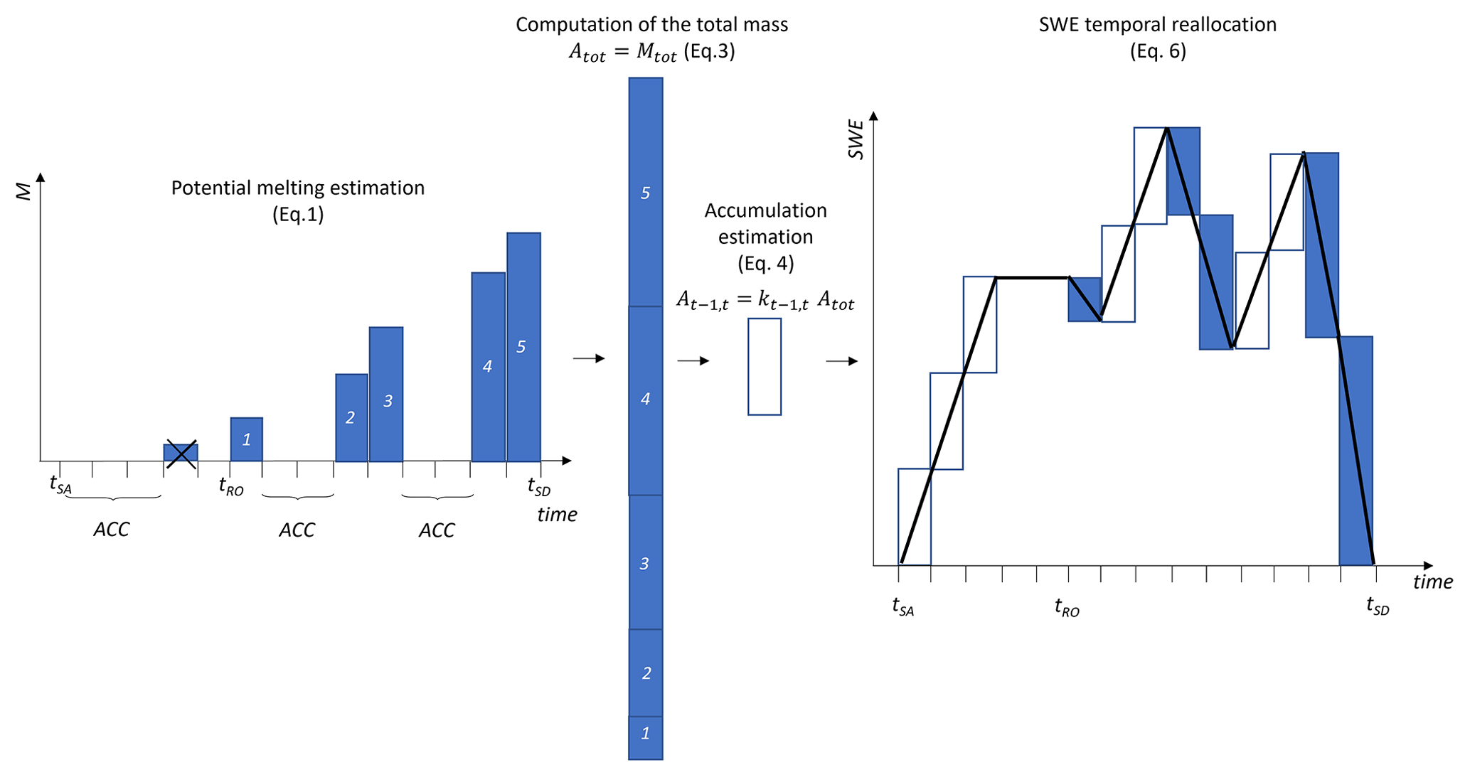
Figure 2Illustration of the reconstruction and temporal reallocation of the SWE for a given pixel. Starting from the left side of the figure, the state is identified for each day of the snow season (delimited by tSA and tSD), and the potential melting is estimated according to Eq. (1). Incorrect melting events prior to the runoff onset are excluded. The sum of all the potential melting on the different days represents the total amount of SWE for that pixel. This is redistributed during the accumulation day using Eq. (4). For this illustrative example, a constant k is considered. As one can notice, the reconstructed SWE can represent accumulation (even as late spring snowfall), ablation, and equilibrium conditions.
To assess the performance of the proposed method, we consider two different test areas. The first one is the South Fork of the San Joaquin River (SFSJR) located in California, USA, in the Sierra Nevada. For this test site, we considered three hydrological seasons that spanned from 1 October 2018 to 30 September 2021. The considered basin has an area of around 970 km2 and a mean elevation of 3070 m, ranging from a minimum elevation of 1930 m to a maximum elevation of 4150 m. The percentage of forest area in this catchment is around 32 % (Shimada et al., 2014). SWE maps with a resolution of 50 m are made available by the Airborne Snow Observatory (ASO). ASO couples an imaging spectrometer, a laser scanner, and a physical model that provides an estimate of the snow density to derive accurate SWE maps (Painter et al., 2016). The product presents an uncertainty derived from both the snow depth retrieval (<0.02 m at a resolution of 50 m) and the snow density modeling (13–30 kg m−3). This dataset represents our main reference for this study, given its high spatial detail comparable with the proposed output. However, we also consider an additional dataset at ∼ 500 m resolution, i.e., the western United States daily snow reanalysis (WUS–SR) product (Fang et al., 2022). A snow pillow for continuous SWE measurements and an AWS providing air temperature are available at the Volcanic Knob (VLC) station, located at an elevation of around 3050 m. Unfortunately, this is the only station within the catchment. For this reason, as explained in Sect. 2.1, we assumed that the accumulation occurs across the entire snow-covered area. However, we also considered six other snow pillows and 10 stations with continuous temperature measurements within a radius of approximately 15 km from the catchment (see Fig. 3a). These data were downloaded from the United States Department of Agriculture (USDA) Natural Resources Conservation Service (NRCS) Snowpack Telemetry (SNOTEL) network (see https://www.wcc.nrcs.usda.gov/snow/, last access: 1 July 2022) and from the California Data Exchange Center (CDEC) (see https://cdec.water.ca.gov/, last access: 1 July 2022).
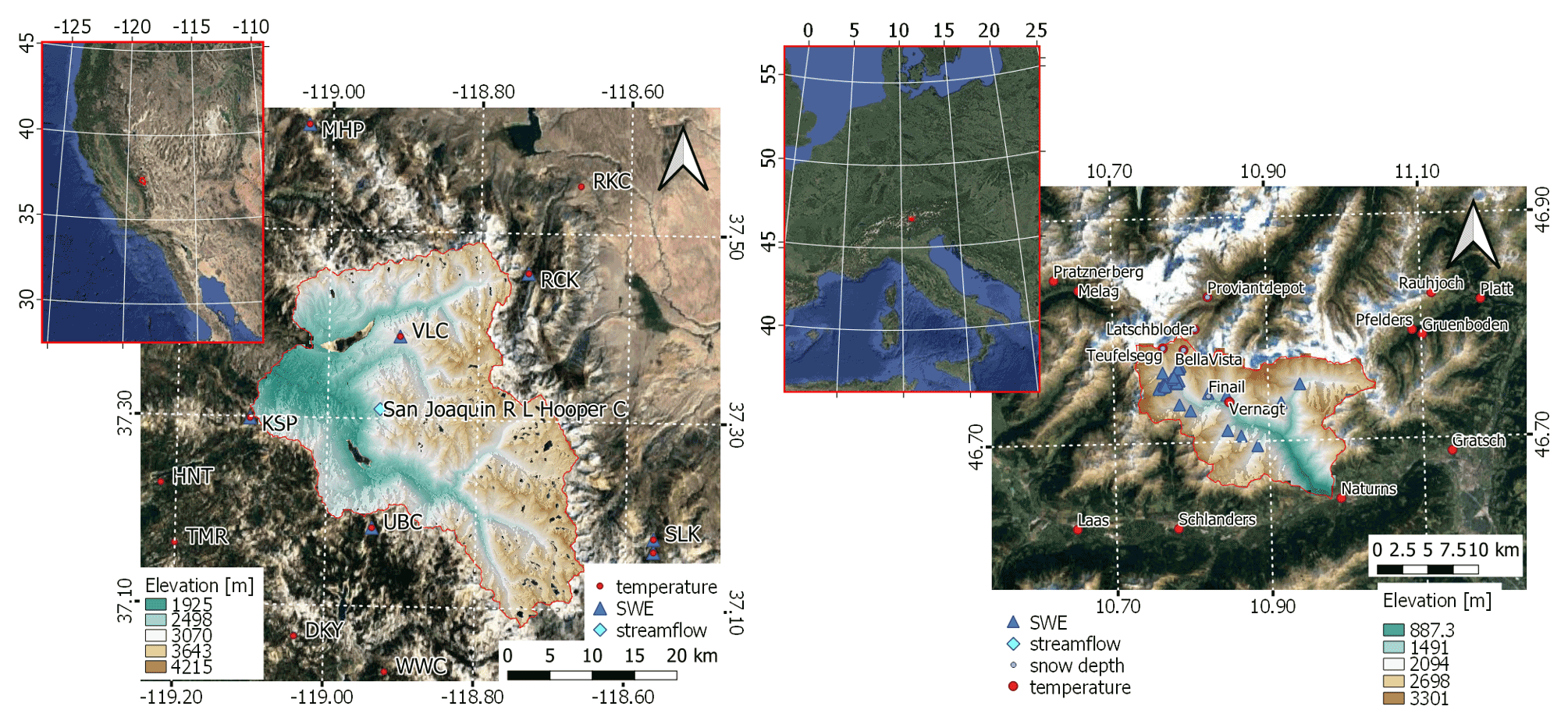
Figure 3Overview of the two test sites: (a) South Fork of the San Joaquin River, California, USA, and (b) Schnals catchment, South Tyrol, Italy. Background image © Google Maps 2022.
The second catchment is the Schnals (Senales in Italian – for brevity we will report the German name only) located in the Vinschgau (Venosta) Valley in South Tyrol (Italy) in the Alps. For this catchment, we analyzed two hydrological seasons spanning from 1 October 2019 to 30 September 2021. The considered area has an extent of approximately 220 km2 and a mean elevation of 2370 m, ranging from a minimum of 590 m up to a maximum of 3550 m. The percentage of forest area is around 25 % for this catchment (Shimada et al., 2014). Manual SWE measurements are available for the hydrological season 2020/2021 (collected by the Avalanche Center of the Bolzano Province – Lawinenwarndienst, see https://lawinen.report/weather/snow-profiles, last access: 1 July 2022; and by Eurac Research, Institute for Earth Observation). Furthermore, we considered the operating temperature and SD sensors of the province of Bozen (see https://data.civis.bz.it/it/dataset/misure-meteo-e-idrografiche, last access: 1 July 2022). An overview of the Schnals catchment and the location of available measurements is provided in Fig. 3b.
The HR daily SCA time series is derived using the method proposed by Premier et al. (2021). The input data used for the reconstruction are the S2, Landsat-8, and MODIS data. The method requires as input a long time series of HR images. Therefore, we downloaded a total of about 400 scenes for SFSJR and 700 scenes for Schnals from https://earthexplorer.usgs.gov (last access: 1 July 2022). The following steps are applied to opportunely preprocess the data: (i) conversion from digital number to top-of-the-atmosphere (ToA) reflectance values, (ii) cloud masking through the algorithm s2cloudless available at https://github.com/sentinel-hub/sentinel2-cloud-detector (last access: 1 July 2022) (Zupanc, 2017), (iii) SCF detection through an unsupervised statistical learning approach (Barella et al., 2022) (RMSE of 22.82 and an MBE of 6.95), and (iv) binarization of the classification results (SCF >10 %). Daily MODIS data are needed for the analyzed hydrological seasons. The ready-to-use MOD10 version 6.1 data are distributed by the National Snow and Ice Data Center (see https://nsidc.org/data/MOD10A1, last access: 1 July 2022) (Hall and Riggs, 2021). The normalized difference snow index (NDSI) values are converted to SCF by using the algorithm proposed by Salomonson and Appel (2004). The output is a daily SCA time series with a spatial resolution of 25 m.
The S1 data are downloaded from https://search.asf.alaska.edu/ (last access: 1 July 2022) and preprocessed (i.e., precise orbit application, thermal noise removal, border noise removal, beta naught calibration, tile assembly, co-registration, multi-temporal filtering, terrain correction, geo-coding, and sigma naught calibration). These steps are performed using SNAP (Sentinel Application Platform) and some custom tools. The images are also resampled at 25 m using the same spatial grid as for the SCA maps. Three tracks are available for each test site, i.e., tracks 64, 137, and 144 for the SFSJR and tracks 15, 117, and 168 for Schnals, with a total number of around 480 and 350 downloaded images, respectively. For this work, we considered the VV polarization only, which is more suitable for runoff onset identification (Marin et al., 2020). The temporal resolution of each separated track is 6 d. For this reason, the backscattering is interpolated daily, and a multi-temporal analysis is carried out for the three tracks separately. If at least one track shows a drop of at least 2 dB in the signal (Nagler and Rott, 2000) with respect to a moving average of the previous 12 d, we look for the minimum after the drop, and for this moment onward the pixel is considered to be in ablation.
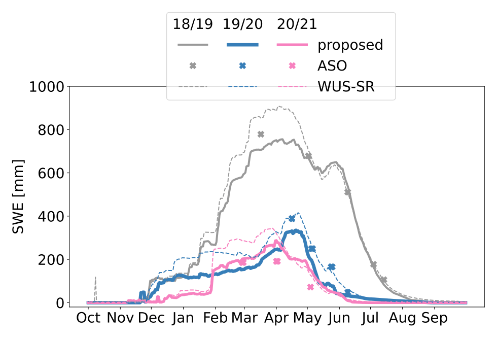
Figure 4Time series of the total SWE for the SFSJR over the three analyzed seasons. Continuous lines represent the proposed time series, dashed lines the WUS–SR dataset, and crosses the ASO reference.
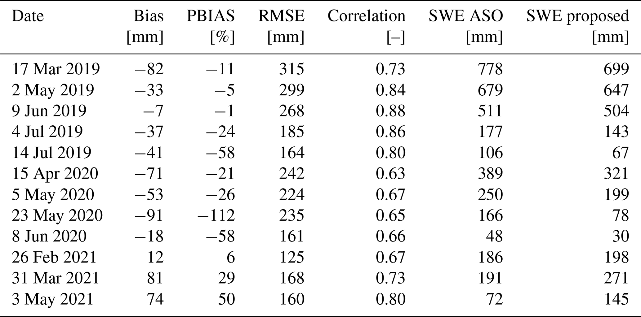
Table 2Results of the intercomparison between the proposed SWE and ASO maps for the SFSJR. Bias, RMSE, and correlation are calculated pixel-wise, while SWE is calculated for the whole basin.
In this section, we present the results obtained for SFSJR and Schnals.
4.1 South Fork of the San Joaquin River
The proposed SWE maps are aggregated at a resolution of 50 m and compared to the corresponding ASO maps, for a total of 12 dates. Furthermore, we also compare the results with the daily western United States snow reanalysis (WUS–SR) dataset at 500 m provided by Fang et al. (2022). The results of the intercomparison with ASO are reported in Table 2. The analysis shows a good correlation between the two products, with an average correlation coefficient of 0.740. The average bias is −22 mm, the average percent bias (PBIAS) is −19 %, and the average RMSE is 212 mm. Our SWE maps underestimate the SWE compared to ASO for the first two seasons, 2018/2019 and 2019/2020, while overestimating it for 2020/2021, which was the driest season with SWE below average (see Sect. S1 and Fig. S1 in the Supplement). A possible explanation is that a drier season leads to earlier melting. As the DD method does not consider seasonality in the DD factor a, it is possible that we overestimate the potential melting during the first phase of the season when melting rates are lower due to less energy radiation input (Musselman et al., 2017; Ismail et al., 2023). Additionally, the five SWE maps from the first season, 2018/2019, show decreasing RMSE values from midwinter to late-summer acquisitions. Larger errors during the midwinter season (around the maximum SWE) are probably due to error propagation (Slater et al., 2013b; Rittger et al., 2016).
Similarly, Table 3 presents the results of the comparison between the proposed SWE dataset and the WUS–SR dataset, for which metrics are computed pixel-wise by aggregating the proposed SWE at a 500 m resolution. An average value is then computed for the entire season. The comparison reveals a systematic negative bias, which may be attributed to the different modeling of snow under the canopy. The correlation between the proposed and WUS–SR datasets is lower than that between the proposed and ASO datasets. For further comparison, Sect. S3 includes additional analyses of the proposed approach, WUS–SR, and ASO at a 500 m resolution. The analysis shows that the WUS–SR dataset also correlates worse with ASO. However, the three time series show a consistent behavior.
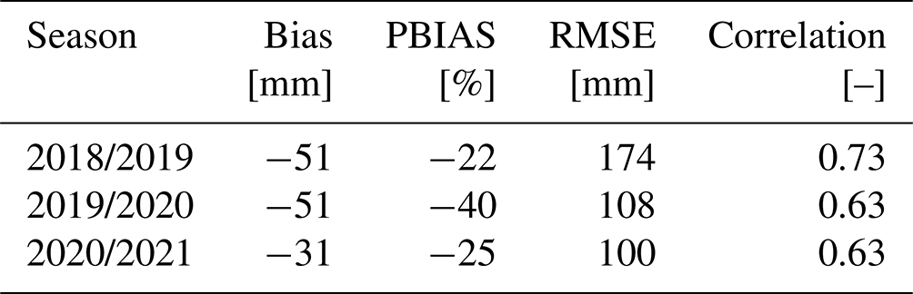
Table 3Results of the intercomparison between the proposed SWE and WUS–SR for the SFSJR. Bias, RMSE, and correlation are calculated pixel-wise. The proposed SWE was aggregated to 500 m resolution.
Good agreement is also confirmed when comparing the total amount of SWE estimated through the three approaches in the catchment. Figure 4 shows the time series of the total SWE for the three hydrological seasons. In the plot, it is possible to appreciate the large SWE variability that can occur for different seasons and that is well represented by all three time series. The first hydrological season 2018/2019 shows the highest amount of SWE, while the others are drier. For reference, the SWE regime for the catchment is reported in Fig. S1.
The VLC monitoring site, which is located within the analyzed area, is also used to evaluate the obtained results, and it shows good agreement between the proposed time series and the in situ measurements (refer to Fig. 5). Note that the WUS–SR presents a delay in detecting the tSD, probably due to the coarser resolution, i.e., 500 m, despite a similar trend. It is worth noting that the first year, 2018/2019, is also used to set up the DD factor a that is then kept constant for the other seasons. The found value is in accordance with numbers present in the literature (Hock, 2003; Ismail et al., 2023). The validity of the chosen value is also confirmed by the good agreement of the results for the next two seasons. However, a delay in detecting tRO is observed in season 2018/2019 that results in a smaller SWE peak.
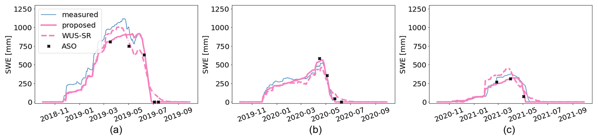
Figure 5SWE obtained by the proposed approach (pink continuous line) is compared against the measured SWE (in blue), the WUS–SR SWE (pink dashed line), and ASO SWE (black crosses) at the Volcanic Knob test site for the hydrological seasons (a) 2018/2019, (b) 2019/2020, and (c) 2020/2021. To extract SWE at the considered location, the original spatial resolution of each dataset is maintained.
We also propose here a more detailed analysis on a specific date. To keep this analysis concise, we propose considering a date during the full melting season, a period of particular interest from a hydrological perspective. The considered date is 9 June 2019. For the analysis on the other dates and the intercomparison with the WUS–SR dataset, please refer to Sect. S3. Figure 6 reports the proposed SWE map, the ASO SWE map, and the bias map calculated as the pixel-wise difference between the proposed and the reference ASO map at 50 m. In general, it is possible to notice good agreement between the two maps. The proposed method is capable of reproducing spatial patterns similar to those detected by ASO. This finding demonstrates that the use of HR input data achieves unique spatial detail, which represents one of the main advantages of the proposed method. Upon closer inspection of a specific area, this similarity can be better appreciated. Nevertheless, it is possible to notice a tendency of the proposed SWE maps to underestimate SWE, especially in some areas exposed to the north. This could be attributed to either (i) an error introduced by the DD model, which only considers temperature and may not account for radiation differences associated with different aspects (Ismail et al., 2023), or (ii) an error in the snow depth retrieval or snow density modeling introduced in the ASO maps.
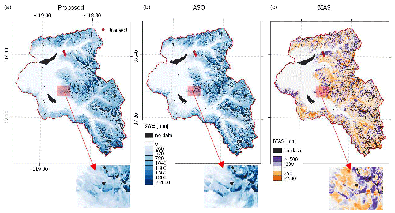
Figure 6Proposed SWE map (a), ASO SWE map (b), and bias map calculated as the difference between the proposed and ASO SWE (c) for 9 June 2019 for the SFSJR. A zoom is shown under the corresponding maps. A transect is shown with three green dots in the northern area of the catchment.
Figure 7a displays the mean SWE values for different elevation, slope, and aspect ranges. The most significant changes are observed when analyzing the different elevation ranges. The trend is quite consistent, with an increase in SWE as elevation increases up to approximately 3500 m a.s.l., while the trend is reversed for higher elevations. These areas generally have very steep slopes, resulting in a marked tendency for snow to be subject to gravitational transport. The two SWE maps only differ for elevations higher than about 4100 m a.s.l., where the proposed SWE starts to increase again, while the ASO continues to decrease. The slope analysis shows larger differences, especially when considering steep slopes. The proposed method underestimates SWE compared to ASO. We generally expect lower SWE for these steeper slopes that promote gravitational transport. The aspect analysis correctly indicates a larger amount of SWE for north-facing areas. As mentioned earlier, we can observe an underestimation of the SWE for north-facing slopes when comparing our maps with the ASO. Conversely, we would expect an overestimation of the SWE for the north-facing areas, as the DD method does not consider radiation effects. However, we never observe this overestimation when considering this and other available reference dates presented in Sect. S3.
Figure 7b shows the dispersion graph for the proposed method and ASO. In general, a strong correlation can be observed, albeit with significant dispersion, which is also confirmed by the computed correlation and RMSE value reported in Table 2. However, the majority of the points are clustered around the diagonal line.
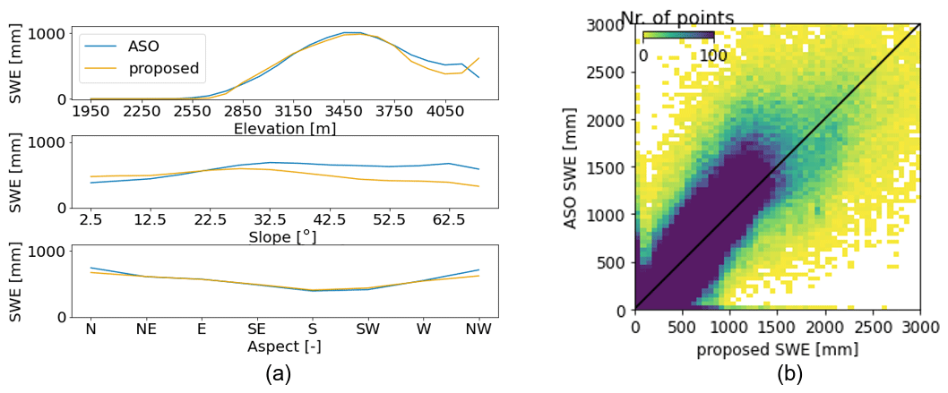
Figure 7Mean SWE value for different elevation, slope, and aspect belts (a). The proposed SWE (in orange) is evaluated against ASO (in blue) for 9 June 2019 for the SFSJR. (b) Dispersion graph for the same date.
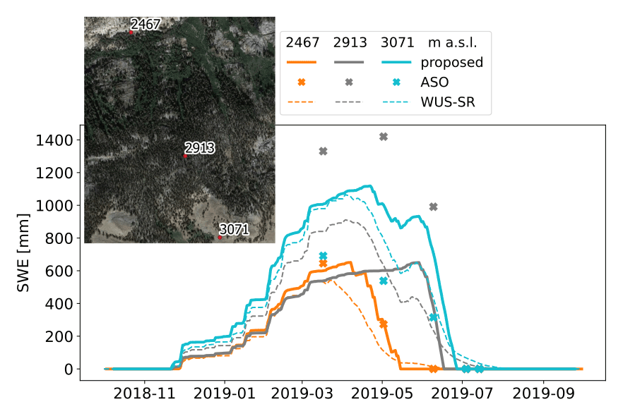
Figure 8The SWE time series in 2018/2019 for the proposed approach (continuous lines), along with WUS–SR (dashed lines) and ASO (crosses) for the same transect. To extract SWE at the considered locations, the original spatial resolution of each dataset is maintained. A zoom of the transect in the SFSJR reported in Fig. 6 is also shown. Background image © Google Maps 2022.
Figure 8b shows the time series for the 2018/2019 season for three points along a selected transect. A zoom of the transect is shown in Fig. 8a (see Fig. 6 for their location in the basin). It is interesting to notice that the three points differ in terms of forest coverage. While the low- and high-elevation points are not directly located in the canopy, this is not the case for the mid-elevation point. The proposed SWE presents an expected behavior, i.e., longer snow persistence and increasing SWE for higher elevation. However, the mid-elevation point shows a later runoff onset with respect to the other points, which is probably due to the fact that the timing detected by S1 is less reliable in that area. This might introduce an underestimation of SWE for that pixel. However, despite some differences that can be due to the different spatial resolution between the two products, an increasing SWE for increasing elevation is also seen for the WUS–SR dataset. On the other hand, the ASO shows a higher SWE for the mid-elevation point. Note that even though we use ASO as a main reference, there may be inconsistencies present, such as possible inaccurate estimation of the snow density by the model. Interestingly, the figure also correctly shows a variability in the three proposed SWE time series. Notwithstanding the fact that the stations are used to identify the accumulation state, the SWE time series does not necessarily present the same shape everywhere as for the station (see Figs. 8 and 5). The final result is influenced not only by the persistence of the snow, but also by the potential melting, which varies depending on the elevation. This is calculated using kriging with external drift.
4.2 Schnals catchment
For the Schnals valley, spatialized SWE data to be used as a reference are unfortunately not available. However, manual SWE measurements for the hydrological season 2020/2021 were collected along spatial transects. The location of the measurements is shown in Fig. 3b. The results show a bias of −5 mm, an RMSE of 191 mm, and a correlation of 0.35. Figure 9 shows the proposed reconstructed SWE plotted against the manual measurements. Despite generally good agreement, we observe some significant differences and a worse performance compared to the analysis performed for the Californian catchment. However, the reference dataset is insufficiently informative and represents only a few points that may not be entirely representative of the intra-pixel variability, especially in complex terrains. As shown by the SWE measurements acquired in Schnalstal by Warscher et al. (2021), high spatial heterogeneity of the SWE can be encountered when considering a pixel with a size of 25 m. This results in inherent difficulties in appropriately evaluating the output.
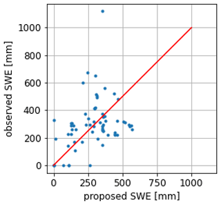
Figure 9Proposed SWE (x axis) against observed SWE (y axis) for the season 2020/2021 in the Schnals catchment (see Fig. 3b).
Figure 10 shows the map of the maximum SWE for the two analyzed hydrological seasons. From these highly detailed maps, it is possible to see that the season 2020/2021 is characterized by a higher amount of SWE. However, the 2 years show similar patterns that are consistent with the morphology of the study area. In detail, we can notice that there is a higher amount of SWE, especially in the eastern part of the catchment, that corresponds to the glacierized area of the Roteck–Monte Rosso mountain. We found a longer persistence of snow for these north-exposed slopes and consequently a larger amount of reconstructed SWE.
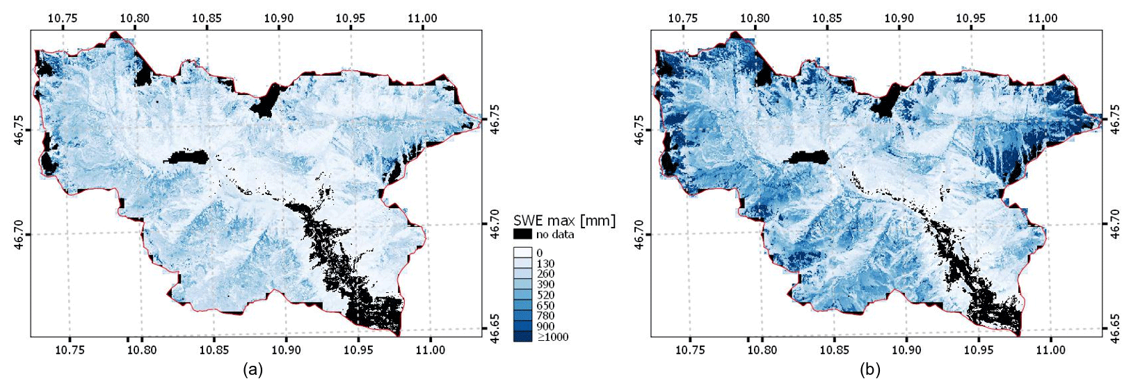
Figure 10Maximum of SWE for the Schnals catchment for the hydrological seasons (a) 2019/2020 and (b) 2020/2021.
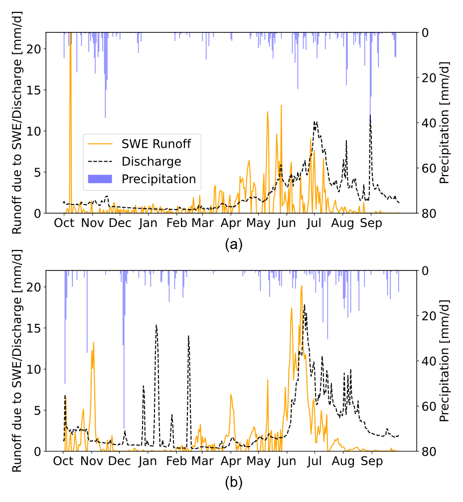
Due to the absence of an appropriate dataset for the SWE intercomparison in the Schnals valley, we carry out a qualitative analysis of the correlation between SWE and riverine discharge. To achieve this, we analyze (i) the discharge measured at Schnalserbach–Gerstgras, (ii) the SWE variations that are associated with runoff (i.e., only when they are associated with a decrease in SWE) for the corresponding subcatchment, and (iii) the precipitation measured at Vernagt. Refer to Fig. 3b for the location of the outlet point and pluviometer. Figure 11 shows good agreement in terms of both timing and quantity between snow-generated runoff and discharge, confirming that the catchment is snowmelt-dominated. The discharge starts increasing in correspondence with the snowmelt, and it starts decreasing when the snowmelt is reduced for both periods. The first year shows a delay, while the response is more direct for the second season. More than differences in terms of precipitation, we ascribe this situation to a different snowmelt rate. Indeed, the season 2019/2020 shows an earlier, weaker, and longer distributed snowmelt period, interrupted by periods with low SWE output (such as the end of March–beginning of April, beginning of May, and middle of June). This situation may favor ground infiltration with a predominance of subsurface runoff with respect to surface runoff, contributing slowly to the discharge. On the other hand, the 2020/2021 season shows a long and high-intensity SWE release (end of May–end of June) that may cause a sudden saturation of the soil, with predominant surface runoff contributing more directly to the discharge. This hypothesis may also be confirmed by recent literature, showing that when snowmelt is earlier, it is also less intense, and the runoff response could be reduced, with strong implications for future climate change impacts (Musselman et al., 2017). However, other contributions should also be considered, such as the storage of water in the two reservoirs present in the territory. While a proper analysis requires a complete hydrological study and a hydraulic characterization of the watershed properties, we believe that this simplified analysis demonstrates the potential of the presented results in a real application.
The results indicate that the proposed method is capable of reproducing the SWE with high geometrical detail and in an accurate way. Particularly good agreement with respect to other datasets is achieved when considering the results on a catchment scale. The method demonstrates good performance in reproducing the expected SWE behavior when analyzing the topography of the study area. However, when considering a reference with comparable spatial resolution, significant differences are observed. In this section, we discuss the main sources of errors and weaknesses that may affect the results and provide a simplified sensitivity analysis of the parameters that play a role in the proposed approach. Furthermore, we also provide a detailed discussion of the effectiveness of the novel SCA regularization introduced through the state definition.
5.1 Sensitivity analysis
The potential sources of errors in the method are represented by (i) a wrong state identification, (ii) the incorrect identification of tSA and tSD, which in turn depends on the accuracy of both the SCA time series and the state, and (iii) the use of a DD model for the potential melting estimation; this in turn depends on the quality of air temperature recordings, the interpolation routines, and the simplified assumption of the method itself, which does not take into account different energy inputs due to either topographical features or different periods of the year. Since the input data are subject to several degrees of preprocessing, it is difficult to perform a complete sensitivity analysis of the method. This has been partially covered by other works (e.g., Slater et al., 2013b; Ismail et al., 2023). Here, we present a simplified sensitivity analysis of the parameters that play a role in the proposed approach. For the sake of clarity, we investigate how the most important parameters affect the final SWE reconstruction by considering the pixel where the station Volcanic Knob provides continuous SWE measurements in the Sierra Nevada catchment. These parameters are (i) the DD factor a, (ii) the SWE threshold SWEmin used to identify the states, (iii) the time of snow disappearance (tSD), (iv) the time of snow appearance (tSA), and (v) the time of the runoff onset detected by S1 (tRO). We vary each of these parameters separately, keeping the others constant and equal to the optimal case (see Table 4). The test is carried out for the 2018/2019 season. Although this analysis is not exhaustive, it gives an overview of the most important sources of error.
Table 4Optimal parameter values for the pixel with the Volcanic Knob station.
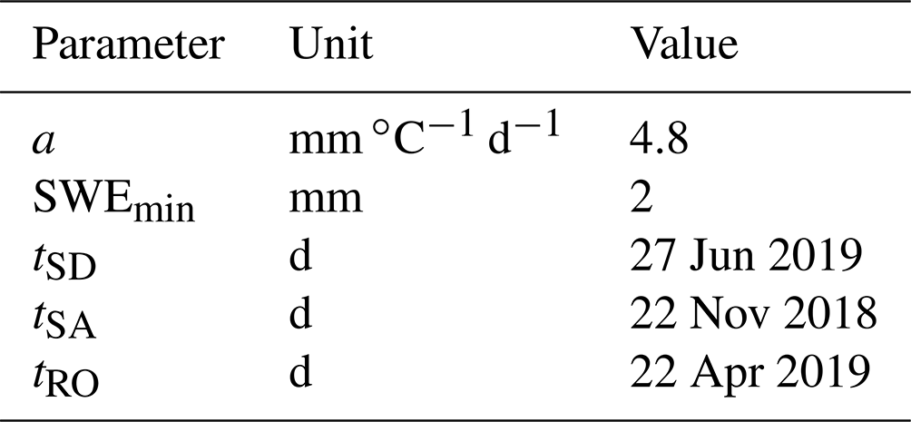
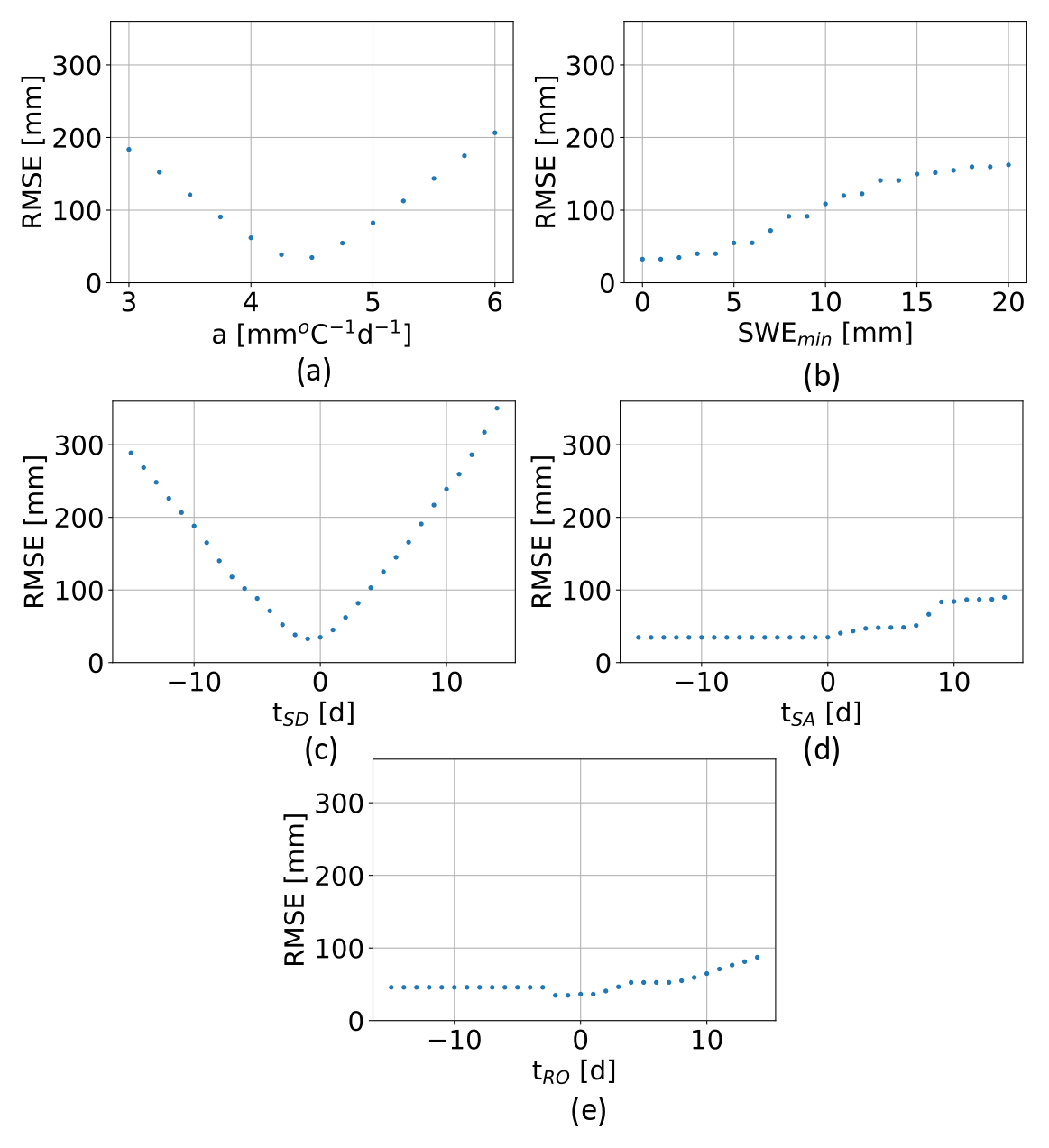
Figure 12Sensitivity analysis of (a) the DD factor (a), (b) the SWE threshold (SWEmin), (c) the time of snow disappearance (tSD), (d) the time of snow appearance (tSA), and (e) the time of the runoff onset detected by S1 (tRO). One parameter is varied while the others are kept constant and equal to the optimal value as reported in Table 4.
In Fig. 12a a varies from 3 to 6 by steps of 0.2 mm ∘C−1 d−1. It is possible to notice that the error increases linearly when a moves away from the optimal value, which is 4.5 mm ∘C−1 d−1, as set for the SWE reconstruction.
In Fig. 12b the SWE threshold varies from 0 to 20 by steps of 1 mm. As expected, the higher the threshold, the greater the error. Indeed, for thresholds that are too large, the method does not detect accumulation states. A snow threshold of 2 mm, as used in this work, is acceptable.
In Fig. 12c tSD varies in a range of ±15 d with respect to the optimal day. Both underestimating and overestimating tSD introduces important errors in the reconstruction. Indeed, at the end of the melting season the temperature is high and consequently the potential melting. A difference of ±5 d (which corresponds to the repetition time of S2) already introduces an RMSE of approximately 50 mm.
In Fig. 12d tSA varies in a range of ±15 d with respect to the optimal day. The shift of tSA does not strongly affect the RMSE as tSD does. For negative shifts, the RMSE is constant since no SWE is added to the reconstruction. Indeed, for these days, we find that the coefficient k (see Eq. 4) is 0 since it is calculated from the AWSs. In other words, it means that the accumulation is not really happening before at least one station detects an increase in SWE. This might introduce an error if some pixels are in accumulation before the station reports it, but it does not affect the maximum amount of SWE for those pixels, which is determined only by the days in ablation.
In Fig. 12e tRO varies in a range of ±15 d with respect to the optimal day. Furthermore, the shift of tRO does not strongly affect the RMSE as does tSD. The RMSE for negative shifts remains constant after a certain point, since for those days Eq. (1) returns zero potential melting due to negative temperatures. This means that anticipating the melting phase is less critical than postponing it, since the temperatures and consequently the potential melting are lower.
In general, we can summarize by stating that changes in a and tSD are expected to strongly affect the results. The DD factor a cannot be considered a constant parameter and has to vary in space and time to minimize the SWE reconstruction error, as pointed out by many researchers (e.g., Ismail et al., 2023). On the other hand, given the high temperature and potential melting values at the end of the ablation, an incorrect estimate of tSD can significantly impact the reconstruction of the SWE peak, resulting in either an overestimation or underestimation. Therefore, the introduction of an accurate daily HR time series can greatly benefit the SWE reconstruction.
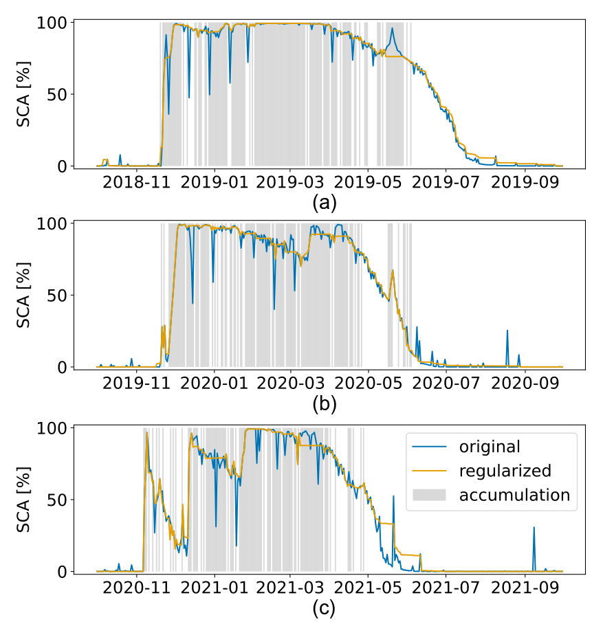
Figure 13SCA time series in the SFSJR for the hydrological seasons (a) 2018/2019, (b) 2019/2020, and (c) 2020/2021. Original input version (in blue) and regularized version (in orange). The gray background color corresponds to an accumulation state.
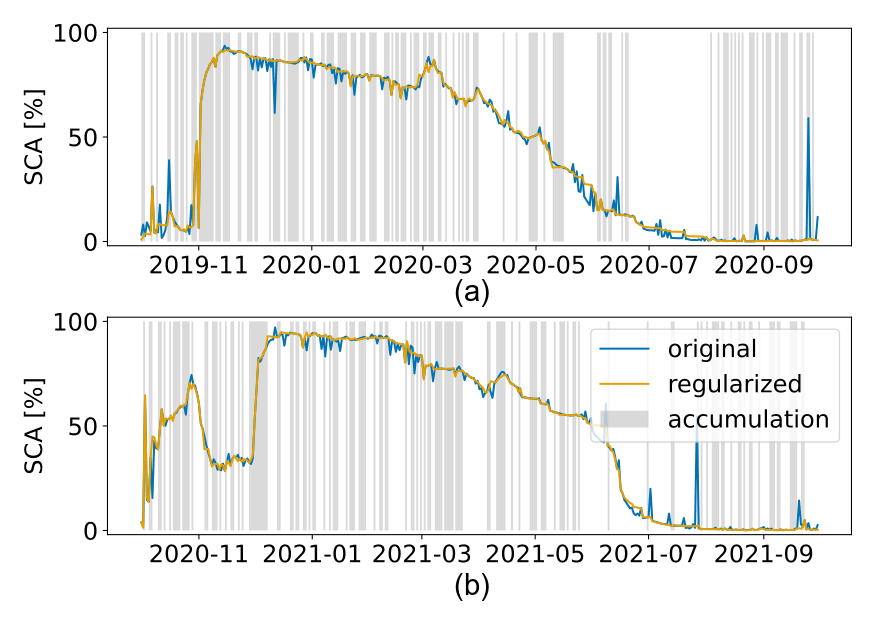
Figure 14SCA time series in the Schnals catchment for the hydrological seasons (a) 2019/2020 and (b) 2020/2021. Original input version (in blue) and regularized version (in orange). The gray background color corresponds to an accumulation state.
5.2 SCA regularization
Figures 13 and 14 show the SCA before and after regularization for the SFSJR and Schnals catchments, respectively. As explained in Sect. 2.2, the raw reconstructed SCA presents two issues: (i) strong decreasing peaks in correspondence with HR acquisitions at the beginning of the season, indicating an underestimation of SCA in forested areas, and (ii) small increasing peaks in correspondence with HR acquisitions in the late melting phase, indicating the presence of snow patches that are not visible in LR images. In contrast, the regularized SCA is more stable, and the spurious oscillations, especially during the coldest winter period, are corrected. The effectiveness of the correction is also visible when looking at the regularized image. Figure 15 represents a common situation in which atmospherically corrupted and mixed pixels are classified erroneously. The proposed correction improves snow detection, especially in these complicated cases.
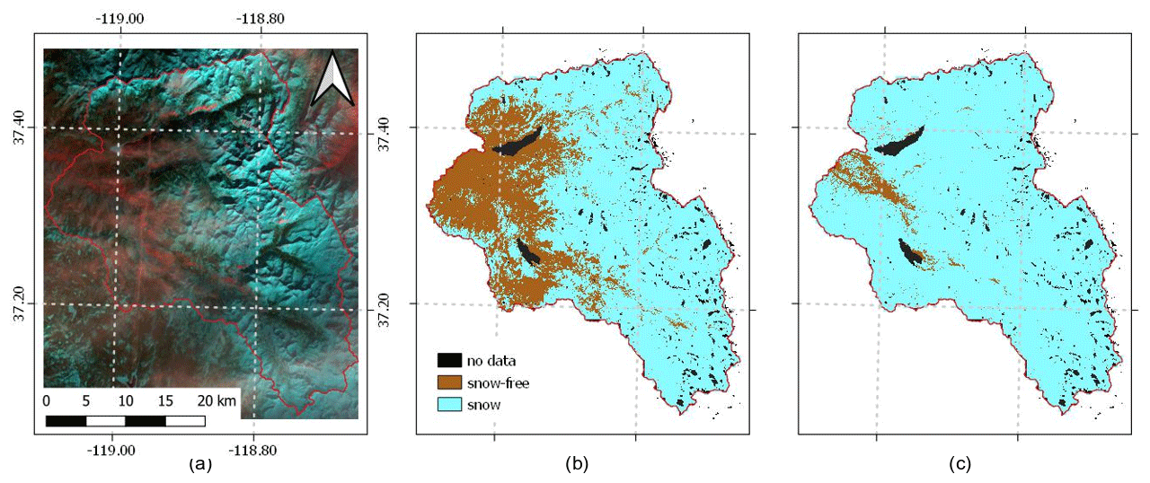
Figure 15Example of a regularized snow map on 12 January 2020 for the SFSJR: (a) false-color composition (R: SWIR, G: NIR, B: RED), (b) original snow cover map, and (c) regularized snow cover map.
An underestimation of SCA is observed in May 2019 for the SFSJR catchment (see Fig. 13a). A careful examination of the conditions that led to the flattening of the SCA during the late snowfall reveals that the stations indicate a long period as accumulation (from 16 to 29 May), whereas the peak starts decreasing in the original SCA time series from 21 May. By applying the rule for a recent snowfall (see Sect. 2.2 and Algorithm 1), the majority of the pixels are labeled as snow-free. In other words, the peak lasts only a few days, so the label snow does not persist for a long time. This implies a replacement with snow-free backward until the day of the last ablation. It is possible that the AWSs present some sensor errors, but this could also be the case of a mixed state inside the catchment. In other words, the AWSs detect snowfall, but this is most likely occurring at high elevations, while the SCA decreases due to ongoing melting or rain on snow, especially in the lower-elevation belts of the catchment. Indeed, the SCA decrease from ∼100 % to ∼80 % means that low elevations become snow-free. However, we expect such ephemeral snowfall not to significantly affect the total amount of SWE, as shown in Sect. 4.1.
On the other hand, an evident case in which an overestimation of the SCA is introduced is in the season 2020/2021 in May–June for the SFSJR (see Fig. 13c). This overestimation is caused by the fact that the AWSs do not indicate an accumulation in correspondence with the peaks that occur in the late melting phase. Therefore, the label is corrected according to the majority rule in ablation in the case of old snowfall. Most of the pixels were snow in previous HR acquisitions, leading to the propagation of the class backward and the consequent overestimation of the SCA. This could be a reason for an overestimation of the SWE as shown in the “Experimental results” section (see Sect. 4.1).
It is evident that the effectiveness of the SCA regularization is strongly influenced by the reliability of the state identification. At the current state, the main limitation of the proposed method is represented by the accumulation identification, which is not provided at a pixel level. Future research should focus on this point and exploit remote sensing observations rather than sparse AWS information. For example, a possible indicator of ongoing accumulation is represented by an SCA increase. However, small variations may be due to errors. Furthermore, snowfall on already snow-covered areas cannot be identified. A possible alternative is represented by the use of SAR data. Recent works have shown that backscattering seems to be sensitive to the presence of fresh snow, showing an increase in the backscattering in correspondence with snowfall (e.g., Tsang et al., 2022; Lievens et al., 2022). However, the poor temporal resolution may strongly affect the accumulation rather then the ablation, since snowfall is expected to be a more rapid phenomenon.
In this work, we explored the use of multi-source satellite data to reconstruct HR daily SWE time series at a spatial resolution of 25 m. The proposed approach involves the following steps: (i) determining the state (i.e., accumulation, ablation, or equilibrium) using in situ SD SWE and temperature observations, as well as S1 multi-temporal backscattering data, (ii) identifying the dates of snow appearance and disappearance from a daily HR snow cover time series derived by fusing high- and low-resolution optical sensors, and (iii) estimating the potential melting from in situ temperature observations using a DD model. We proposed a novel regularization of the SCA time series that considers the state information. The regularization corrects impossible transitions, i.e., erroneous changes in the pixel class from snow to snow-free when in accumulation or equilibrium and, vice versa, from snow-free to snow when in ablation and equilibrium. Finally, the SWE is added or removed from the reconstruction according to the state, with the amount determined by the potential melting calculated using the DD model.
The proposed novel state concept is utilized throughout the different steps of the method, resulting in an SWE reconstruction that incorporates the accumulation phase and potential late snowfall. Furthermore, spatialized precipitation data, which can be unreliable for complex terrains, are not required as the method redistributes the amount of melting by leveraging state information rather than quantifying precipitation input. The state also enables the implementation of a new regularization of the SCA time series. Additionally, the use of a daily HR SCA time series in combination with melting phase information from SAR data is introduced as a further innovation.
The method was tested in two mountainous catchments: (i) the SFSJR, located in the Sierra Nevada – California (USA), and (ii) the Schnals catchment, located in the Alps – South Tyrol (Italy). The results obtained demonstrated the effectiveness of the proposed approach in estimating HR SWE. For the first catchment, the results were evaluated against ASO SWE at 50 m, showing an average bias of −22 mm, an RMSE of 212 mm, and a correlation of 0.74. When evaluated against the daily WUS–SR dataset at 500 m resolution, they showed a bias of −44 mm, an RMSE of 127 mm, and a correlation of 0.66. For the second site, the results were evaluated against manual measurements, showing a bias of −5 mm, an RMSE of 191 mm, and a correlation of 0.35. The obtained results were extensively discussed, considering possible hydrological applications of such a dataset. In this sense, we showed that the results are very promising since they (i) are able to capture the typical spatial variability of an HR map, (ii) show spatial patterns that are consistent with a reference with comparable spatial resolution, as well as with the topography of the study area, (iii) provide consistent trends when considering the basin scale, (iv) reproduce the variability of different hydrological seasons, and (v) require limited meteorological and ground snow observations.
The main sources of error are discussed to provide insights into the main advantages and disadvantages of the method that may be of great interest for several hydrological and ecological applications. It was found that the main sources of errors arise from the potential melting calculation and from the time of snow disappearance. To address potential melting errors, we presented a method that incorporates spatialized information from S1 to determine when the snowpack is subject to runoff and prevent false early melting. Secondly, we introduced the use of HR SCA for SWE reconstruction, which is more adequate to sample the SCA variations due to the complex topography of mountainous catchments. Technological limitations are still present, such as the necessity of merging LR and HR sensors given the absence of daily optical HR acquisitions, the absence of an appropriate observation to determine the accumulation state pixel-wise, and the scarce temporal resolution of SAR acquisitions. Although the proposed approach attempts to overcome all these limitations, we expect that further improvements will also be introduced by future satellite missions, such as Copernicus LSTM and ROSE-L, which will acquire new important information for SWE retrieval. This will not only improve the proposed method but also enable the development of near-real-time predictors of SWE for large hydrological and ecological applications.
The implemented code can be made available upon request to the authors. All the raw input data are freely available as indicated in Sect. 3. The output dataset related to this article is available in the repository at https://doi.org/10.5281/zenodo.8036793 (Premier et al., 2023), or it can be requested directly from the authors.
The supplement related to this article is available online at: https://doi.org/10.5194/tc-17-2387-2023-supplement.
VP and CM designed the research; VP carried out the experiments and processing; RB provided the HR snow maps from S2; all the authors contributed to the analysis and interpretation of the results; VP wrote the paper based on inputs and feedbacks from all coauthors.
The contact author has declared that none of the authors has any competing interests.
Publisher's note: Copernicus Publications remains neutral with regard to jurisdictional claims in published maps and institutional affiliations.
This work was supported by a joint project of the Swiss National Science Foundation (SNF) and Autonomous Province of Bolzano (Italy) – “Snowtinel: Sentinel-1 SAR assisted catchment hydrology: toward an improved snow-melt dynamics for alpine regions” (contract no. 200021L_205190). The authors thank the Department of Innovation, Research and University of the Autonomous Province of Bozen/Bolzano for covering the open-access publication costs. We would also like to thank the NASA Airborne Snow Observatory (ASO) and the NASA National Snow and Ice Data Center for providing free-of-charge data.
This research has been supported by the Schweizerischer Nationalfonds zur Förderung der Wissenschaftlichen Forschung (grant no. 200021L_205190).
This paper was edited by Edward Bair and reviewed by Noah Molotch and two anonymous referees.
Anderton, S., White, S., and Alvera, B.: Micro-scale spatial variability and the timing of snow melt runoff in a high mountain catchment, J. Hydrol., 268, 158–176, 2002. a
Archer, D. and Stewart, D.: The Installation and Use of a Snow Pillow to Monitor Snow Water Equivalent, Water Environ. Manage, 9, 221–230, https://doi.org/10.1111/j.1747-6593.1995.tb00934.x, 1995. a
Arsenault, K. R. and Houser, P. R.: Generating observation-based snow depletion curves for use in snow cover data assimilation, Geosciences, 8, 484, https://doi.org/10.3390/geosciences8120484, 2018. a
Baghdadi, N., Gauthier, Y., and Bernier, M.: Capability of multitemporal ERS-1 SAR data for wet-snow mapping, Remote Sens. Environ., 60, 174–186, 1997. a
Bair, E. H., Rittger, K., Davis, R. E., Painter, T. H., and Dozier, J.: Validating reconstruction of snow water equivalent in California's Sierra Nevada using measurements from the NASA Airborne Snow Observatory, Water Resour. Res., 52, 8437–8460, https://doi.org/10.1002/2016WR018704, 2016. a, b
Balk, B. and Elder, K.: Combining binary decision tree and geostatistical methods to estimate snow distribution in a mountain watershed, Water Resour. Res., 36, 13–26, 2000. a
Barella, R., Marin, C., Gianinetto, M., and Notarnicola, C.: A novel approach to high resolution snow cover fraction retrieval in mountainous regions, in: IGARSS 2022–2022 IEEE International Geoscience and Remote Sensing Symposium, 3856–3859, IEEE, 2022. a
Beniston, M., Farinotti, D., Stoffel, M., Andreassen, L. M., Coppola, E., Eckert, N., Fantini, A., Giacona, F., Hauck, C., Huss, M., Huwald, H., Lehning, M., López-Moreno, J.-I., Magnusson, J., Marty, C., Morán-Tejéda, E., Morin, S., Naaim, M., Provenzale, A., Rabatel, A., Six, D., Stötter, J., Strasser, U., Terzago, S., and Vincent, C.: The European mountain cryosphere: a review of its current state, trends, and future challenges, The Cryosphere, 12, 759–794, https://doi.org/10.5194/tc-12-759-2018, 2018. a
Cline, D. W., Bales, R. C., and Dozier, J.: Estimating the spatial distribution of snow in mountain basins using remote sensing and energy balance modeling, Water Resour. Res., 34, 1275–1285, 1998. a
Darychuk, S. E., Shea, J. M., Menounos, B., Chesnokova, A., Jost, G., and Weber, F.: Snowmelt characterization from optical and synthetic-aperture radar observations in the La Joie Basin, British Columbia, The Cryosphere, 17, 1457–1473, https://doi.org/10.5194/tc-17-1457-2023, 2023. a
Deschamps-Berger, C., Gascoin, S., Berthier, E., Deems, J., Gutmann, E., Dehecq, A., Shean, D., and Dumont, M.: Snow depth mapping from stereo satellite imagery in mountainous terrain: evaluation using airborne laser-scanning data, The Cryosphere, 14, 2925–2940, https://doi.org/10.5194/tc-14-2925-2020, 2020. a
DeWalle, D. and Rango, A.: Modelling snowmelt runoff, Principles of Snow Hydrology. Cambridge University Press, New York, USA, 266–305, 2008. a
Dietz, A. J., Kuenzer, C., Gessner, U., and Dech, S.: Remote sensing of snow–a review of available methods, Int. J. Remote Sens., 33, 4094–4134, 2012. a
Dong, C.: Remote sensing, hydrological modeling and in situ observations in snow cover research: A review, J. Hydrol., 561, 573–583, 2018. a
Durand, M., Molotch, N. P., and Margulis, S. A.: Merging complementary remote sensing datasets in the context of snow water equivalent reconstruction, Remote Sens. Environ., 112, 1212–1225, 2008. a
Endrizzi, S., Gruber, S., Dall'Amico, M., and Rigon, R.: GEOtop 2.0: simulating the combined energy and water balance at and below the land surface accounting for soil freezing, snow cover and terrain effects, Geosci. Model Dev., 7, 2831–2857, https://doi.org/10.5194/gmd-7-2831-2014, 2014. a
Engel, M., Notarnicola, C., Endrizzi, S., and Bertoldi, G.: Snow model sensitivity analysis to understand spatial and temporal snow dynamics in a high-elevation catchment, Hydrol. Process., 31, 4151–4168, 2017. a, b
Fang, Y., Liu, Y., and Margulis, S.: Western United States UCLA Daily Snow Reanalysis, Version 1.[Indicate subset used], Boulder, Colorado USA. NASA National Snow and Ice Data Center Distributed Active Archive Center [data set], https://doi.org/10.5067/PP7T2GBI52I2, 760, 2022. a, b
Fehlmann, M., Gascón, E., Rohrer, M., Schwarb, M., and Stoffel, M.: Estimating the snowfall limit in alpine and pre-alpine valleys: A local evaluation of operational approaches, Atmos. Res., 204, 136–148, 2018. a
Guneriussen, T., Hogda, K. A., Johnsen, H., and Lauknes, I.: InSAR for estimation of changes in snow water equivalent of dry snow, IEEE T. Geosci. Remote, 39, 2101–2108, 2001. a
Günther, D., Marke, T., Essery, R., and Strasser, U.: Uncertainties in snowpack simulations – Assessing the impact of model structure, parameter choice, and forcing data error on point-scale energy balance snow model performance, Water Resour. Res., 55, 2779–2800, 2019. a
Hall, D. K. and Riggs, G. A.: MODIS/Aqua Snow Cover Daily L3 Global 500 m SIN Grid, Version 61. 2021, NASA National Snow and Ice Data Center Distributed Active Archive Center [data set], https://doi.org/10.5067/MODIS/MYD10A1.061 (last access: 1 July 2022), 2021. a
Helfricht, K., Hartl, L., Koch, R., Marty, C., and Olefs, M.: Obtaining sub-daily new snow density from automated measurements in high mountain regions, Hydrol. Earth Syst. Sci., 22, 2655–2668, https://doi.org/10.5194/hess-22-2655-2018, 2018. a
Hock, R.: Temperature index melt modelling in mountain areas, J. Hydrol., 282, 104–115, https://doi.org/10.1016/S0022-1694(03)00257-9, 2003. a, b
Immerzeel, W. W., Lutz, A. F., Andrade, M., Bahl, A., Biemans, H., Bolch, T., Hyde, S., Brumby, S., Davies, B. J., Elmore, A. C., Emmer, A., Feng, M., Fernández, A., Haritashya, U., Kargel, J. S., Koppes, M., Kraaijenbrink, P. D. A., Kulkarni, A. V., Mayewski, P. A., Nepal, S., Pacheco, P., Painter, T. H., Pellicciotti, F., Rajaram, H., Rupper, S., Sinisalo, A., Shrestha, A. B., Viviroli, D., Wada, Y., Xiao, C., Yao, T., and Baillie, J. E. M.: Importance and vulnerability of the world’s water towers, Nature, 577, 364–369, 2020. a
Ismail, M. F., Bogacki, W., Disse, M., Schäfer, M., and Kirschbauer, L.: Estimating degree-day factors of snow based on energy flux components, The Cryosphere, 17, 211–231, https://doi.org/10.5194/tc-17-211-2023, 2023. a, b, c, d, e, f
Jost, G., Weiler, M., Gluns, D. R., and Alila, Y.: The influence of forest and topography on snow accumulation and melt at the watershed-scale, J. Hydrol., 347, 101–115, 2007. a
Lehning, M., Völksch, I., Gustafsson, D., Nguyen, T. A., Stähli, M., and Zappa, M.: ALPINE3D: a detailed model of mountain surface processes and its application to snow hydrology, Hydrol. Process., 20, 2111–2128, 2006. a
Leinss, S., Wiesmann, A., Lemmetyinen, J., and Hajnsek, I.: Snow water equivalent of dry snow measured by differential interferometry, IEEE J. Sel. Top. Appli. Earth Obs., 8, 3773–3790, 2015. a
Li, D., Lettenmaier, D. P., Margulis, S. A., and Andreadis, K.: The value of accurate high-resolution and spatially continuous snow information to streamflow forecasts, J. Hydrometeorol., 20, 731–749, 2019. a
Lievens, H., Brangers, I., Marshall, H.-P., Jonas, T., Olefs, M., and De Lannoy, G.: Sentinel-1 snow depth retrieval at sub-kilometer resolution over the European Alps, The Cryosphere, 16, 159–177, https://doi.org/10.5194/tc-16-159-2022, 2022. a
Luce, C. H., Tarboton, D. G., and Cooley, K. R.: The influence of the spatial distribution of snow on basin-averaged snowmelt, Hydrol. Process., 12, 1671–1683, 1998. a
Marin, C., Bertoldi, G., Premier, V., Callegari, M., Brida, C., Hürkamp, K., Tschiersch, J., Zebisch, M., and Notarnicola, C.: Use of Sentinel-1 radar observations to evaluate snowmelt dynamics in alpine regions, The Cryosphere, 14, 935–956, https://doi.org/10.5194/tc-14-935-2020, 2020. a, b, c, d
Martinec, J. and Rango, A.: Areal Distribution of Snow Water Equivalent Evaluated by Snow Cover Monitoring, Water Resour. Res., 17, 1480–1488, https://doi.org/10.1029/WR017i005p01480, 1981. a, b, c
Meløysund, V., Leira, B., Høiseth, K. V., and Lisø, K. R.: Predicting snow density using meteorological data, Meteorol. Appl., 14, 413–423, 2007. a
Mendoza, P. A., Musselman, K. N., Revuelto, J., Deems, J. S., López-Moreno, J. I., and McPhee, J.: Interannual and seasonal variability of snow depth scaling behavior in a subalpine catchment, Water Resour. Res., 56, e2020WR027343, https://doi.org/10.1029/2020WR027343, 2020. a
Molotch, N. P. and Bales, R. C.: Scaling snow observations from the point to the grid element: Implications for observation network design, Water Resour. Res., 41, https://doi.org/10.1029/2005WR004229, 2005. a
Molotch, N. P. and Bales, R. C.: Comparison of ground-based and airborne snow surface albedo parameterizations in an alpine watershed: Impact on snowpack mass balance, Water Resour. Res., 42, https://doi.org/10.1029/2005WR004522, 2006. a
Molotch, N. P. and Margulis, S. A.: Estimating the distribution of snow water equivalent using remotely sensed snow cover data and a spatially distributed snowmelt model: A multi-resolution, multi-sensor comparison, Adv. Water Resour., 31, 1503–1514, 2008. a, b, c
Molotch, N. P., Painter, T. H., Bales, R. C., and Dozier, J.: Incorporating remotely-sensed snow albedo into a spatially-distributed snowmelt model, Geophys. Res. Lett., 31, https://doi.org/10.1029/2003GL019063, 2004. a
Mott, R., Vionnet, V., and Grünewald, T.: The seasonal snow cover dynamics: review on wind-driven coupling processes, Front. Earth Sci., 6, 197, https://doi.org/10.3389/feart.2018.00197, 2018. a
Murphy, B., Yurchak, R., and Müller, S.: GeoStat-Framework/PyKrige: v1.5.0 (Version v1.5.0), Zenodo [data set], https://doi.org/10.5281/zenodo.3739879 (last access: 1 July 2022), 2020. a
Musselman, K. N., Clark, M. P., Liu, C., Ikeda, K., and Rasmussen, R.: Slower snowmelt in a warmer world, Nat. Clim. Change, 7, 214–219, 2017. a, b
Nagler, T. and Rott, H.: Retrieval of wet snow by means of multitemporal SAR data, IEEE T. Geosci. Remote, 38, 754–765, 2000. a, b
Ohmura, A.: Physical basis for the temperature-based melt-index method, J. Appl. Meteorol. Climatol., 40, 753–761, 2001. a
Painter, T. H., Berisford, D. F., Boardman, J. W., Bormann, K. J., Deems, J. S., Gehrke, F., Hedrick, A., Joyce, M., Laidlaw, R., Marks, D., Mattmann, C., McGurk, B., Ramirez, P., Richardson, M., McKenzie Skiles, S., Seidel, F. C., and Winstral, A.: The Airborne Snow Observatory: Fusion of scanning lidar, imaging spectrometer, and physically-based modeling for mapping snow water equivalent and snow albedo, Remote Sens. Environ., 184, 139–152, 2016. a, b
Parajka, J. and Blöschl, G.: Validation of MODIS snow cover images over Austria, Hydrol. Earth Syst. Sci., 10, 679–689, https://doi.org/10.5194/hess-10-679-2006, 2006. a, b
Pimentel, R., Herrero, J., Zeng, Y., Su, Z., and Polo, M. J.: Study of snow dynamics at subgrid scale in semiarid environments combining terrestrial photography and data assimilation techniques, J. Hydrometeorol., 16, 563–578, 2015. a
Pimentel, R., Herrero, J., and Polo, M. J.: Subgrid parameterization of snow distribution at a Mediterranean site using terrestrial photography, Hydrol. Earth Syst. Sci., 21, 805–820, https://doi.org/10.5194/hess-21-805-2017, 2017. a
Prein, A. F. and Gobiet, A.: Impacts of uncertainties in European gridded precipitation observations on regional climate analysis, Int. J. Climatol., 37, 305–327, 2017. a
Premier, V., Marin, C., Steger, S., Notarnicola, C., and Bruzzone, L.: A Novel Approach Based on a Hierarchical Multiresolution Analysis of Optical Time Series to Reconstruct the Daily High-Resolution Snow Cover Area, IEEE J. Sel. Top. Appl. Earth Obs., 14, 9223–9240, 2021. a, b, c, d
Premier, V., Marin, C., Bertoldi, G., Barella, R., Notarnicola, C., and Bruzzone, L.: Snow Water Equivalent Dataset for the South Fork of the San Joaquin River (2018/2021) and Senales (2019/2021) (Version v0), Zenodo [data set], https://doi.org/10.5281/zenodo.8036793, 2023. a
Pulliainen, J., Luojus, K., Derksen, C., Mudryk, L., Lemmetyinen, J., Salminen, M., Ikonen, J., Takala, M., Cohen, J., Smolander, T., and Norberg, J.: Patterns and trends of Northern Hemisphere snow mass from 1980 to 2018, Nature, 581, 294–298, 2020. a
Rees, W. G.: Remote sensing of snow and ice, CRC Press, Boca Raton, Florida, 285 pp., 2005. a
Revuelto, J., Alonso-González, E., Gascoin, S., Rodríguez-López, G., and López-Moreno, J. I.: Spatial Downscaling of MODIS Snow Cover Observations Using Sentinel-2 Snow Products, Remote Sens., 13, 4513, https://doi.org/10.3390/rs13224513, 2021. a
Rittger, K., Bair, E. H., Kahl, A., and Dozier, J.: Spatial estimates of snow water equivalent from reconstruction, Adv. Water Resour., 94, 345–363, https://doi.org/10.1016/j.advwatres.2016.05.015, 2016. a, b
Rott, H., Yueh, S. H., Cline, D. W., Duguay, C., Essery, R., Haas, C., Hélière, F., Kern, M., Macelloni, G., Malnes, E., Nagler, T., Pulliainen, J., Rebhan, H., and Thompson, A.: Cold regions hydrology high-resolution observatory for snow and cold land processes, Proc. IEEE, 98, 752–765, 2010. a
Salomonson, V. V. and Appel, I.: Estimating fractional snow cover from MODIS using the normalized difference snow index, Remote Sens. Environ., 89, 351–360, 2004. a
Schattan, P., Köhli, M., Schrön, M., Baroni, G., and Oswald, S. E.: Sensing area-average snow water equivalent with cosmic-ray neutrons: The influence of fractional snow cover, Water Resour. Res., 55, 10796–10812, 2019. a
Shi, J., Dozier, J., and Rott, H.: Snow mapping in alpine regions with synthetic aperture radar, IEEE T. Geosci. Remote, 32, 152–158, 1994. a
Shimada, M., Itoh, T., Motooka, T., Watanabe, M., Shiraishi, T., Thapa, R., and Lucas, R.: New global forest/non-forest maps from ALOS PALSAR data (2007–2010), Remote Sens. Environ., 155, 13–31, 2014. a, b
Slater, A., Barrett, A., Clark, M., Lundquist, J., and Raleigh, M.: Uncertainty in seasonal snow reconstruction: Relative impacts of model forcing and image availability, Adv. Water Resour., 55, 165–177, https://doi.org/10.1016/j.advwatres.2012.07.006, 2013a. a
Slater, A., Barrett, A., Clark, M., Lundquist, J., and Raleigh, M.: Uncertainty in seasonal snow reconstruction: Relative impacts of model forcing and image availability, Adv. Water Resour., 55, 165–177, 2013b. a, b
Tsang, L., Durand, M., Derksen, C., Barros, A. P., Kang, D.-H., Lievens, H., Marshall, H.-P., Zhu, J., Johnson, J., King, J., Lemmetyinen, J., Sandells, M., Rutter, N., Siqueira, P., Nolin, A., Osmanoglu, B., Vuyovich, C., Kim, E., Taylor, D., Merkouriadi, I., Brucker, L., Navari, M., Dumont, M., Kelly, R., Kim, R. S., Liao, T.-H., Borah, F., and Xu, X.: Review article: Global monitoring of snow water equivalent using high-frequency radar remote sensing, The Cryosphere, 16, 3531–3573, https://doi.org/10.5194/tc-16-3531-2022, 2022. a, b
Ulaby, F. T., Moore, R. K., and Fung, A. K.: Microwave Remote Sensing: Active and Passive, Vol I, Microwave remote sensing fundamentals and radiometry, Artech House, Norwood, MA, 456–456, 1981. a
Vionnet, V., Brun, E., Morin, S., Boone, A., Faroux, S., Le Moigne, P., Martin, E., and Willemet, J.-M.: The detailed snowpack scheme Crocus and its implementation in SURFEX v7.2, Geosci. Model Dev., 5, 773–791, https://doi.org/10.5194/gmd-5-773-2012, 2012. a
Viviroli, D., Weingartner, R., and Messerli, B.: Assessing the hydrological significance of the world's mountains, Mountain Res. Dev., 23, 32–40, 2003. a
Warscher, M., Marke, T., and Strasser, U.: Operational and experimental snow observation systems in the upper Rofental: data from 2017–2020, Earth Syst. Sci. Data Discuss. [preprint], https://doi.org/10.5194/essd-2021-68, 2021. a
Yang, K., Musselman, K. N., Rittger, K., Margulis, S. A., Painter, T. H., and Molotch, N. P.: Combining ground-based and remotely sensed snow data in a linear regression model for real-time estimation of snow water equivalent, Adv. Water Resour., 160, 104075, https://doi.org/10.1016/j.advwatres.2021.104075, 2022. a
Zupanc, A.: Improving cloud detection with machine learning, https://medium.com/sentinel-hub/improving-cloud-detection-with-machine-learning-c09dc5d7cf13 (last access: 1 July 2022), 2017. a