Constraining regional glacier reconstructions using past ice thickness of deglaciating areas – a case study in the European Alps

In order to assess future glacier evolution and meltwater runoff, accurate knowledge on the volume and the ice thickness distribution of glaciers is crucial. However, in situ observations of glacier thickness are sparse in many regions worldwide due to the difficulty of undertaking field surveys. This lack of in situ measurements can be partially overcome by remote-sensing information. Multi-temporal and contemporaneous data on glacier extent and surface elevation provide past information on ice thickness for retreating glaciers in the newly deglacierized regions. However, these observations are concentrated near the glacier snouts, which is disadvantageous because it is known to introduce biases in ice thickness reconstruction approaches. Here, we show a strategy to overcome this generic limitation of so-called retreat thickness observations by applying an empirical relationship between the ice viscosity at locations with in situ observations and observations from digital elevation model (DEM) differencing at the glacier margins. Various datasets from the European Alps are combined to model the ice thickness distribution of Alpine glaciers for two time steps (1970 and 2003) based on the observed thickness in regions uncovered from ice during the study period. Our results show that the average ice thickness would be substantially underestimated (∼ 40 %) when relying solely on thickness observations from previously glacierized areas. Thus, a transferable topography-based viscosity scaling is developed to correct the modelled ice thickness distribution. It is shown that the presented approach is able to reproduce region-wide glacier volumes, although larger uncertainties remain at a local scale, and thus might represent a powerful tool for application in regions with sparse observations.

1 Introduction

Glaciers are retreating in most mountain regions of the world due to climate warming. Recent measurements of global glacier change show that around 20 % of the observed sea-level rise during the 21st century can be attributed to mass loss of mountain glaciers (Hugonnet et al., 2021). Moreover, diminishing glacier volumes affect seasonal water runoff and the availability of fresh water (Huss and Hock, 2018; Rodell et al., 2018), particularly in arid and semiarid regions. At the local scale, glacier retreat induces natural hazards related to periglacial and glacial environments (Stoffel and Huggel, 2012), such as rockfalls or flooding, but could also offer new hydrological storage and sustainable energy potentials (Ehrbar et al., 2018; Farinotti et al., 2019b). Therefore, knowledge of the distribution of glacier ice volume and thickness is crucial to predict future glacier retreat and deglacierization as well as the subsequent consequences on freshwater supply, hazards (glacial lake outburst floods) and sea level (Marzeion et al., 2012). While increasingly detailed glacier area inventories are becoming available (Pfeffer et al., 2014), there are still no direct measurements of ice thickness for the majority of the glaciers (Welty et al., 2020). Furthermore, modelling approaches with respect to the glacier-wide thickness distribution and volume are also required for glaciers with direct observations of ice thickness, as in situ measurements typically only cover a fraction of the glacierized area (Farinotti et al., 2021).

To efficiently derive the thickness of glaciers on a regional scale, the Ice Thickness Models Intercomparison eXperiment (ITMIX) aimed at the comparison of different thickness reconstruction approaches, solely based on properties of the glacier surface (Farinotti et al., 2017). Participating models were diverse and relied on mass conservation, simplifications of the force balance, the perfect plasticity assumption or a combination of these. Historically, many of the approaches did not aim at reproducing available thickness measurements. These primarily entered as loose calibration or validation observations. Therefore, during the second experimental phase (ITMIX2), the intercomparison was extended to include ice thickness measurements, and it tested the capability of these approaches to assimilate thickness observations. While the inclusion of thickness observations did improve the average modelled ice thickness, the results suggest that an uneven distribution of observations across the glacier domain can cause a systematic bias in ice thickness. Particularly, an underestimation of average glacier thickness was found for several models when relying preferentially on thickness observations of the lowest glacier elevations. Contrastingly, measurements of the thick glacier parts reduced the spread in estimated mean thickness between the ITMIX2 members (Farinotti et al., 2021). Similarly, a recent study, based on remote-sensing glacier velocity measurements and an inversion approach of Stokes ice flow mechanics (Jouvet, 2022), showed that the availability of ice thickness observations, although less important for estimates of total glacier volumes, can greatly improve the modelled ice thickness distribution.

However, this poses a problem for thickness estimations of many glaciers, as in situ observations of ice thickness, such as direct measurements by drilling, seismic soundings or ground-penetrating radar (GPR), are usually associated with considerable logistical efforts and technical challenges. Nevertheless, ice thickness for a given previous glacier geometry is readily available for the deglacierized region from remote sensing. Glacier inventories and digital elevation models (DEMs) provide information on the extent and surface elevation. When comparing glacier outlines at different time steps, once glacierized areas that became ice-free between the acquisition dates of glacier inventories can be identified. The original ice thickness is then estimated by differencing the respective DEMs. With the growing number of available glacier outline and elevation datasets for different moments of time (Paul et al., 2020), these observations, hereafter termed “retreat thickness observations”, will increasingly become available. This information is a large asset for calibrating reconstruction approaches in many regions without in situ thickness measurements. Even though some local inconsistencies related to changes in terrain elevation after deglaciation due to erosion and sedimentation processes might be present, the uncertainty in surface elevation inferred by remote sensing is typically much smaller than a direct measurement of ice thickness (e.g. by GPR), and complete information on former ice thickness in deglaciated areas is available. Therefore, retreat thickness observations have a considerable potential to improve ice thickness estimates for the entire glacier.

Here, we present an approach to reconstruct the glacier-wide ice thickness distribution and volume from thickness observations based on repeated DEMs in deglacierized areas. To avoid a potential underestimation of the mean ice thickness, the model is calibrated with a slope- and elevation-based rescaling of the ice viscosity. The reconstruction is based on Alpine glaciers, as glacier monitoring activities in the European Alps are more intense and denser than anywhere else in the world (Haeberli et al., 2007; WGMS, 2021). We use glacier inventories and DEMs to identify areas at the glacier margins that have become ice-free since the 1970s and extract the prior ice thickness by differencing the respective DEMs. Additionally, empirical viscosity scaling parameters are derived from a large number of available in situ measurements of ice thickness, compiled from various sources. The 1970s ice thickness distribution of Swiss and Austrian glaciers is then reconstructed based on remote-sensing data for the period from ∼1970 to 2019 as well as different subsets of thickness observations from field surveys and deglacierized areas. Finally, the approach is transferred to all Alpine glaciers, and the modelled ice thickness of the early 21st century is compared to previous reconstructions of Alpine glacier volumes.

2 Data and methods

The ice thickness distribution of Alpine glaciers is calculated following the ice thickness reconstruction proposed by Fürst et al. (2017, 2018). The reconstruction is based on mass conservation, adapted from Morlighem et al. (2011), and relies on the principle of the shallow-ice approximation (SIA) (Hutter, 1983). Initially, the glacier-wide ice flux is derived from the difference between the surface mass balance (SMB) and the surface elevation change. Thereafter, the estimated ice flow is converted to ice thickness, assuming the SIA. SIA-based approaches have been used by a number of recent regional to global glacier thickness reconstructions (Farinotti et al., 2019a; Maussion et al., 2019; Millan et al., 2022). Here, the applied reconstruction by Fürst et al. (2017) showed a close resemblance to locally observed ice thickness and robust thickness estimates during the ITMIX2 intercomparison if thickness observations were provided (Farinotti et al., 2021).

2.1 Ice thickness reconstruction

The mass conservation of the ice flow is expressed as a vertical integral following Eq. (1) (Cuffey and Paterson, 2010):

$$\begin{array}{}\text{(1)}& {\displaystyle \frac{\mathit{\delta }H}{\mathit{\delta }t}}+\mathrm{\nabla }\cdot \left(uH\right)={\dot{b}}_{\mathrm{S}}+{\dot{b}}_{\mathrm{b}},\end{array}$$

where ∇ is the two-dimensional divergence operator; H is the ice thickness; u denotes the vertically averaged, horizontal velocity components; $\frac{\mathit{\delta }H}{\mathit{\delta }t}$ represents the glacier surface height changes; and ${\dot{\mathrm{b}}}_{\mathrm{S}}$ and ${\dot{\mathrm{b}}}_{\mathrm{b}}$ are the surface and basal mass balance, respectively. The product of u and H is equal to the ice flux F.

Eventually, the glacier-wide flux F is translated into local ice thickness according to Eq. (2), assuming the SIA (Hutter, 1983):

$$\begin{array}{}\text{(2)}& F^{\ast }={\displaystyle \frac{\mathrm{2}}{n+\mathrm{2}}}{\mathit{\eta }}^{-n}{\left(\mathit{\rho }g\right)}^n\mathrm{|}\left|\mathrm{\nabla }h\right|{\mathrm{|}}^n\cdot H^{n+\mathrm{2}}.\end{array}$$

The two-dimensional flux field solution is determined over the entire drainage basin, as defined by the glacier compound outline. Here, n is the flow law exponent, ρ is the density of ice (917 kg m⁻³), g is the gravitational acceleration (9.18 m s⁻²) and η is the ice viscosity.

2.2 Viscosity scaling

Motivated by spatial uncertainties when estimating ice thickness from lateral measurements (Farinotti et al., 2021), the mass conservation approach was extended by including the dependencies of ice viscosity and surface slope (Carrivick et al., 2016) and elevation. Therefore, η is calibrated according to slope- and elevation-dependent scaling factors (Eq. 3):

$$\begin{array}{}\text{(3)}& \mathit{\eta }={\mathit{\eta }}_{\mathrm{0}}\cdot \left({\mathit{\xi }}_{\mathit{\eta }}^{\mathrm{slope}}\cdot {\mathit{\xi }}_{\mathit{\eta }}^{\mathrm{elevation}}\cdot {\mathit{\xi }}_{\mathit{\eta }}^{\mathrm{distance}}\right).\end{array}$$

Here, η₀ is the initially estimated viscosity, which is multiplied by correction factors for the surface slope ${\mathit{\xi }}_{\mathit{\eta }}^{\mathrm{slope}}$ (Sect. 3.2) and glacier elevation range ${\mathit{\xi }}_{\mathit{\eta }}^{\mathrm{elevation}}$ (Sect. 3.3), and ${\mathit{\xi }}_{\mathit{\eta }}^{\mathrm{distance}}$ is an additional scaling factor based on the distance to the glacier margin (Eq. 4):

$$\begin{array}{}\text{(4)}& {\mathit{\xi }}_{\mathit{\eta }}^{\mathrm{distance}}=\text{atan}\left({\displaystyle \frac{d_{\mathrm{margin}}}{\mathrm{4}\cdot H}}\right)\times {\displaystyle \frac{\mathrm{2}}{\mathit{\pi }}},\end{array}$$

where d_margin is the distance to the glacier margin.

The ice viscosity η₀ is initially estimated at locations where ice thickness measurements are available. It is then interpolated across the glacier domain. To better constrain η₀ at the domain margins and avoid extrapolation artefacts, the mean viscosity from all measurements is prescribed around the glacier outline. For glaciers without any thickness measurements, the mean region-wide viscosity is used.

2.3 Uncertainty estimate

The uncertainty in the reconstructed ice thickness distribution and derived glacier volumes is estimated based on a formal error map. These error maps include contributions from the uncertainties in the input SMB (Sect. 2.4.5) and $\frac{\mathit{\delta }H}{\mathit{\delta }t}$ (Sect. 2.4.2) information. Using those uncertainties, the flux error is estimated and converted into thickness uncertainty fields (Eq. 2). At locations with ice thickness observations, the thickness error map is set to the respective measurement uncertainty. To avoid artefacts in the error maps, unrealistically high uncertainty values are replaced by the glacier-specific median ice thickness in cases where the local uncertainty is higher than the median ice thickness. A detailed description of the formal error estimation can be found in Fürst et al. (2017).

2.4 Input datasets

2.4.1 Ice surface elevation

Concerning the elevations of Alpine glaciers, past and present surface heights are derived from aerial photography, digitized topographic maps and spaceborne synthetic aperture radar (SAR) DEMs. For the Austrian Alps, aerial photographs of all glacierized areas were acquired with a mean picture scale of 1:30 000 between September and October 1969 (Patzelt, 1980). The original images were later digitized and co-registered to derive the photogrammetric DHM69 elevation model (Lambrecht and Kuhn, 2007) that is used in this study. Historic glacier elevations of the Swiss Alps are available via the DHM25 dataset provided by the Federal Office of Topography swisstopo (Anonymous, 2005). The DHM25 elevation model was created from the Swiss national topographic map (scale 1:25 000) by digitizing contour lines and spot heights which were then interpolated to a 25 m resolution grid. We use the original DHM25lvl1 product, because glacier areas were updated with surface heights from winter 2000/2001 in the DHM25lvl2. Most map tiles covering the central Swiss Alps are from the 1980s (Anonymous, 2005), but the dates of glacier heights differ from the DHM25 specifications. Therefore, we refer to a detailed manual reconstruction (Fischer et al., 2015a) of the specific reference years (1961–1991) of the DHM25 to derive the map date of each glacier. For the early 21st century, glacier surface topography is extracted from the 1 arcsec void-filled C-band SAR DEM of the Shuttle Radar Topography Mission (SRTM; Farr et al., 2007; Podest and Crow, 2013), which was acquired during February 2000. Recent glacier surface heights are provided by the bistatic TanDEM-X (TerraSAR-X add-on for Digital Elevation Measurement) satellite mission, operated by the German Aerospace Center (DLR) (Krieger et al., 2007; Zink et al., 2016). We use SAR DEMs from winter 2013/2014 (Sommer et al., 2020) and 2018/2019 to derive respective elevation mosaics. The 2018/2019 TanDEM-X DEMs were created from ∼160 co-registered single-look slant-range complex (CoSSC) acquisitions using differential interferometry and were vertically and horizontally co-registered according to the workflow described by Sommer et al. (2020). In this study, all elevation datasets are resampled to 30 m grids.

2.4.2 Surface elevation changes

The 1969–2019 elevation changes in Austrian glaciers are inferred from the DHM69 and TanDEM-X. The TanDEM-X DEM and the DHM69 are vertically and horizontally co-registered, using non-glacierized and flat terrain (slope < 15^∘) outside glacierized areas and waterbodies (Braun et al., 2019). Eventually, the DEMs are differenced and elevation change rates ($\frac{\mathit{\delta }H}{\mathit{\delta }t}$) are calculated from the TanDEM-X and DHM69 acquisition dates. As the DHM69 was acquired between September and October 1969, we use the average date (1 October 1969) as a reference date. For the Swiss Alps, glacier elevation changes are obtained by differencing the TanDEM-X 2018/2019 DEM mosaic and the DHM25. As for the DHM69, the TanDEM-X DEM and the DHM25 are vertically and horizontally co-registered to minimize elevation offsets. Thereafter, we use the individual glacier reference years of the DHM25 (Fischer et al., 2015a) (Sect. 2.3.1) and the TanDEM-X acquisition dates to convert the height difference into elevation change rates. The median observation period of all Swiss glaciers is 1975–2019, with glacier-specific periods varying between 1961–2019 and 1991–2019. For the later reconstruction period (2000–2014), we use glacier elevation change rates derived from differencing SRTM C-band (February 2000) and TanDEM-X DEMs of winter 2013/2014 (Sommer et al., 2020). In most cases, data voids in the elevation change maps are caused by SAR layover and shadows. Therefore, we apply a bilinear interpolation, as recommended by a recent study (Seehaus et al., 2020). Finally, all elevation change fields are bilinearly resampled to a spatial resolution of 30 m.

The mean vertical precision of the glacier elevation change rate is derived as slope-dependent standard deviations on non-glacierized areas. All elevation change values outside glacier areas are aggregated within 5^∘ slope bins. Thereafter, standard deviations of each slope bin are calculated and weighted by the respective total glacier area to derive the region-wide mean uncertainty. Further details on the elevation change error calculation are described in Sommer et al. (2020). For the DEM differences of the DHM25, DHM69 and the 2019 TanDEM-X acquisitions, the mean regional elevation change uncertainty is ±0.26 and ±0.18 m a⁻¹, respectively, which represents an uncertainty of ∼39 % relative to the measured absolute elevation change over the entire observation period. The slope-derived $\frac{\mathit{\delta }H}{\mathit{\delta }t}$ error of the 2000–2014 period is ±0.39 m a⁻¹ (Sommer et al., 2020), with a relative uncertainty of ∼53 %. Therefore, we use an average uncertainty in the elevation change fields of ±0.3 m a⁻¹. It should be noted that we did not attempt a correction for height offsets between the optical/topographic and SAR DEMs due to signal penetration into the glacier surface. Particularly, for the DEM difference between the 2018/2019 TanDEM-X DEMs of winter 2018/2019 and DHM69 of autumn 1969, glacier surface elevations were acquired during different seasons, and the presence of signal penetration is likely for the TanDEM-X DEMs. However, we assume that the bias in elevation change due to radar penetration is small, as the snow cover of winter 2018/2019 is probably partially invisible for the X-band SAR, and the observation period is very long (∼40 years). In the case of the DHM25, no correction is applied because the exact mapping dates of the glacier areas are unknown.

2.4.3 Glacier outlines

The 20th century outlines of Alpine glaciers are extracted from the 1969 Austrian glacier inventory (GI1) and the 1973 Swiss glacier inventory (SGI1973). The 1969 Austrian GI1 was originally compiled from the same aerial photographs as the DHM69 (Patzelt, 1980) and later digitized (Lambrecht and Kuhn, 2007). Outlines of the SGI1973 are based on aerial photographs of September 1973 (Müller et al., 1976; Maisch et al., 2000) that were digitized and georeferenced by Paul et al. (2004). Due to the varying timestamps of the DHM25, many glacier outlines of the SGI1973 are older than the respective surface heights of the DHM25. However, the glacier area change between 1973 and 1985 was very small ($\sim -\mathrm{1}$ %) (Paul et al., 2004). Several glacier inventories covering the entire Alps have been created from satellite images and semiautomatic classification. The Randolph Glacier Inventory (RGI) (Pfeffer et al., 2014) of the European Alps was mostly created from band ratios of optical 2003 Landsat imagery with a resolution of 30 m (Paul et al., 2011). The 2013–2015 glacier extents were mapped from Landsat 8 images (Sommer et al., 2020). The most recent Alps-wide inventory is based on 10 m resolution Sentinel-2 acquisitions (Paul et al., 2020) from the years 2015–2017. Additionally, recent regional inventories, based on the manual delineation of glacier outlines from high-resolution optical images and elevation models, are available for the Austrian Alps for 2015 (Buckel et al., 2018) and for the Swiss Alps for 2013–2018 (SGI2016) (Linsbauer et al., 2021). For each glacier inventory, adjacent glacier boundaries are removed and the respective glaciers are merged into continuous geometries, thereby avoiding inconsistencies in ice thickness across divides and ridges (Fürst et al., 2017).

2.4.4 Ice thickness observations

Reference ice thickness observations of Alpine glaciers are available via the Glacier Thickness Database (GlaThiDa v3) (GlaThiDa Consortium, 2020), which is a standardized collection of remote sensing and in situ measurements, and a recent publication on helicopter-borne ground-penetrating radar (GPR) measurements of almost all larger Swiss glaciers (Grab et al., 2021). While the GlaThiDa database of Alpine glaciers includes a large number of observations from different time periods and measurement techniques, the dataset by Grab et al. (2021) provides mainly GPR tracks between 2016 and 2020 but also older, so far not publicly available, measurements. Most of the in situ thickness observations are very densely spaced. Therefore, we removed observations that were less than 30 m apart, resulting in a total number of ∼53 000 in situ measurements. The mean measurement uncertainty of all in situ observations is 8.2 m or ∼10 % relative to the mean glacier thickness of all in situ observations. For ∼30 % of the observations, the error is unknown because there is no information on the measurement uncertainty within the GlaThiDa database. For those measurements, the uncertainty is approximated as 20 % of the respective ice thickness value.

Thickness observations of the glacier margins are derived from glacier areas that became ice-free, as delineated by the multi-temporal outline and elevation information. Therefore, absolute elevation change values (δH) are extracted at glacier retreat areas that were inferred from differencing the respective glacier inventories. Additionally, an inner and outer buffer of 30 m is applied to the glacier retreat areas, and a slope threshold of 25^∘ is enforced to exclude values close to the glacier outlines or on steeper slopes, as these values tend to be less reliable. In summary, we derive approximately 140 000 thickness observations from glacier areas that became ice-free between 1969 (Austria – AT) and ∼1970 (Switzerland – CH) and 2019. For the 2000–2014 period, we obtain 70 000 observations. The uncertainty in the δH measurements can be estimated from the errors in the $\frac{\mathit{\delta }H}{\mathit{\delta }t}$ fields (Sect. 2.4.2) and the respective observations periods of the DEM differences. Hence, the mean vertical δH uncertainties for the ∼1970–2019 period are ±10.3 and ±8.9 m for Swiss and Austrian glaciers, whereas they are ±5.5 m for the 2000–2014 period. Compared with the respective mean δH, the relative uncertainty in the retreat thickness measurements is ∼34 % (AT) and 38 % (CH) for ∼1970–2019 and ∼25 % (Alps) for 2000–2014.

2.4.5 Surface mass balance

SMB estimates for all glaciers of the European Alps (referring to the RGI v6.0) are available from the Global Glacier Evolution Model (GloGEM) (Huss and Hock, 2015; Zekollari et al., 2019). The model describes the main processes of mass balance – accumulation, melt and refreezing – and provides the annual SMB for 10 m elevation bins between 1951 and 2019. The model was driven by the E-OBS dataset (Cornes et al., 2018) and has been calibrated to match glacier-specific mass changes for 2000–2019 (Hugonnet et al., 2021). For the ice thickness reconstruction in this study, we averaged the annual SMB of each glacier over the 1969–2019 and 2000–2014 periods, respectively. The elevation-binned SMB information is transferred to 30 m grids using linear interpolation. To account for variations in glacier area and elevation over time, we use the SRTM DEM and RGI outlines for the 2000–2014 period and the Swiss and Austrian glacier inventories (GI1 and SGI1973) as well as surface elevations of the DHM69 and DHM25 for ∼1970–2019. For the historic glacier inventories (GI1 and SGI1973), we spatially matched the glacier areas and the IDs of the RGI by comparing the respective outlines. In cases where the historic outline overlapped with more than one RGI ID, due to differences in the delineation of ice divides or the disintegration of a once continuous glacierized area into several smaller glaciers, we used the SMB values of the RGI geometry that had the largest spatial overlap. In addition, we had to apply hypsometric extrapolation in some cases to vertically extend the SMB information, as the glacier outline of the historic inventories covered a larger elevation range than the respective RGI geometry.

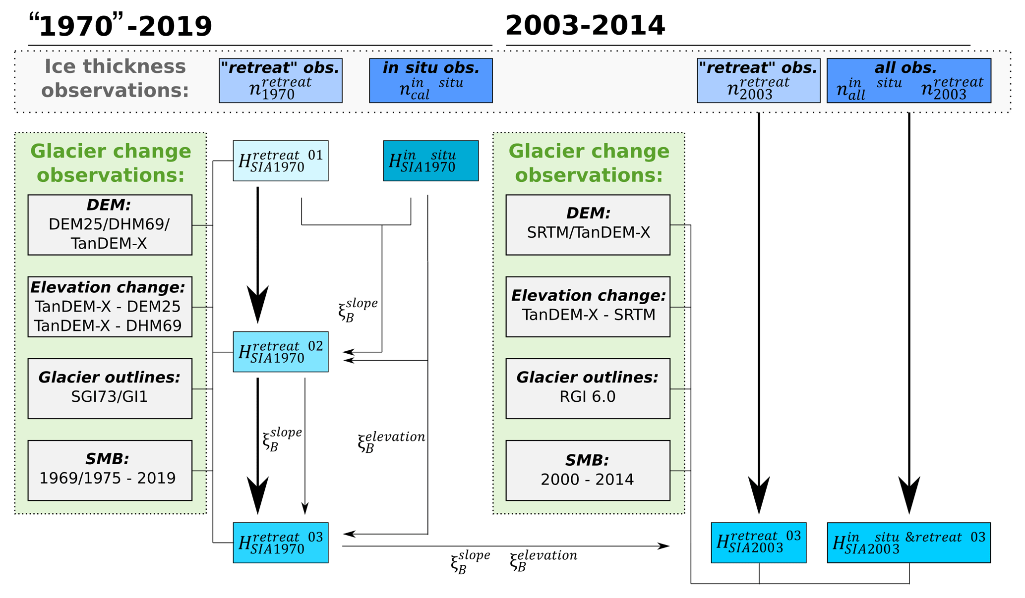
Figure 1 Visualization of the experimental set-up and input datasets: over the 1970–2019 period, surface slope- and elevation-based scaling factors (${\mathit{\xi }}_{\mathit{\eta }}^{\mathrm{slope}}$ and ${\mathit{\xi }}_{\mathit{\eta }}^{\mathrm{elevation}}$, respectively) are calibrated by comparing the ice thickness distribution (H_SIA1970) derived from in situ thickness observations ($H_{\mathrm{SIA}\mathrm{1970}}^{\mathrm{in}\mathrm{situ}}$) and retreat thickness observations at the glacier margins ($H_{\mathrm{SIA}\mathrm{1970}}^{\mathrm{retreat}}$). By iterating $H_{\mathrm{SIA}\mathrm{1970}}^{\mathrm{retreat}}$ ($H_{\mathrm{SIA}\mathrm{1970}}^{\mathrm{retreat}\mathrm{01}}$ – $H_{\mathrm{SIA}\mathrm{1970}}^{\mathrm{retreat}\mathrm{03}}$), ${\mathit{\xi }}_{\mathit{\eta }}^{\mathrm{slope}}$ and ${\mathit{\xi }}_{\mathit{\eta }}^{\mathrm{elevation}}$ are calibrated. Eventually, the calibrated scaling factors (${\mathit{\xi }}_{\mathit{\eta }}^{\mathrm{slope}}$ and ${\mathit{\xi }}_{\mathit{\eta }}^{\mathrm{elevation}}$) are transferred to the 2003–2014 period to estimate the total Alps-wide glacier volume from different samples of ice thickness observations ($H_{\mathrm{SIA}\mathrm{2003}}^{\mathrm{in}\mathrm{situ}\mathrm{\&}\mathrm{retreat}\mathrm{03}}$ and $H_{\mathrm{SIA}\mathrm{2003}}^{\mathrm{retreat}\mathrm{03}}$).

2.5 Experimental set-up

For the mass conservation reconstruction, information on the glacier extent, surface topography, and surface mass balance and elevation changes are required. Additional thickness observations are used to constrain the estimated ice thickness. Based on the above presented input datasets, we first calibrate the reconstruction method during the full observational period from 1970 to 2019 in Switzerland and Austria. The method is then transferred to the entire European Alps focussing on the 2000–2014 period. A detailed overview of the experimental set-up and the input datasets used is shown in Fig. 1 and described in detail in the following sections.

2.5.1 Reconstruction calibration for 1970–2019

For the early period from 1969 to 1973, glacier heights are extracted from the Swiss DHM25 and Austrian DHM69, and glacier areas are taken from the SGI1973 and GI1. The acquisition dates of the respective glacier outlines mostly refer to the years 1973 (CH) and 1969 (AT). Regarding the glacier surface topography, the Austrian DHM69 represents surface heights for the same year as the glacier inventory, whereas the Swiss DHM25 elevations refer to regionally different acquisition years (see Sect. 2.3.1). Thus, in the following sections, the reconstruction of the historic Swiss and Austrian ice thickness is denoted as H_SIA1970, according to the approximate acquisition dates of the glacier outlines and DEMs (1970). As input fields for the H_SIA1970 reconstruction, elevation change rates are derived from the difference between the DHM25/DHM69 and TanDEM-X mosaic for winter 2018/2019. The H_SIA1970 is applied for two experimental set-ups using different samples of thickness observations and viscosity scaling factors.

For the initial reference run ($H_{\mathrm{SIA}\mathrm{1970}}^{\text{in situ}}$), the available in situ thickness observations (GlaThiDa Consortium, 2020; Grab et al., 2021) of glaciers in the Swiss and Austrian Alps are divided into two equal subsamples. All glaciers with in situ measurements (304 glaciers total) are grouped into four classes of equal size using the glacier area quantiles. Thereafter, half of the glaciers in each class are selected randomly to create a set of calibration and validation glaciers (152 glaciers each). Based on those randomly selected glaciers, the in situ thickness observations are divided into a set of calibration ($n_{\mathrm{cal}}^{\text{in situ}}=\mathrm{24}\mathrm{677}$ measurements) and validation ($n_{\mathrm{val}}^{\text{in situ}}=\mathrm{25}\mathrm{753}$ measurements) points. The thickness measurements of these observational datasets are rather equally distributed across lower and upper sections of the glaciers and provide a good representation of both the thick and central parts as well as the glacier margins. A detailed overview of the random selection of calibration and validation glaciers is provided in Tables S1 and S2 and Figs. S1 and S2 in the Supplement. All in situ thickness observations of the 152 calibration glaciers are used for $H_{\mathrm{SIA}\mathrm{1970}}^{\text{in situ}}$. No scaling of the ice viscosity is applied (Figs. 1, 2a).

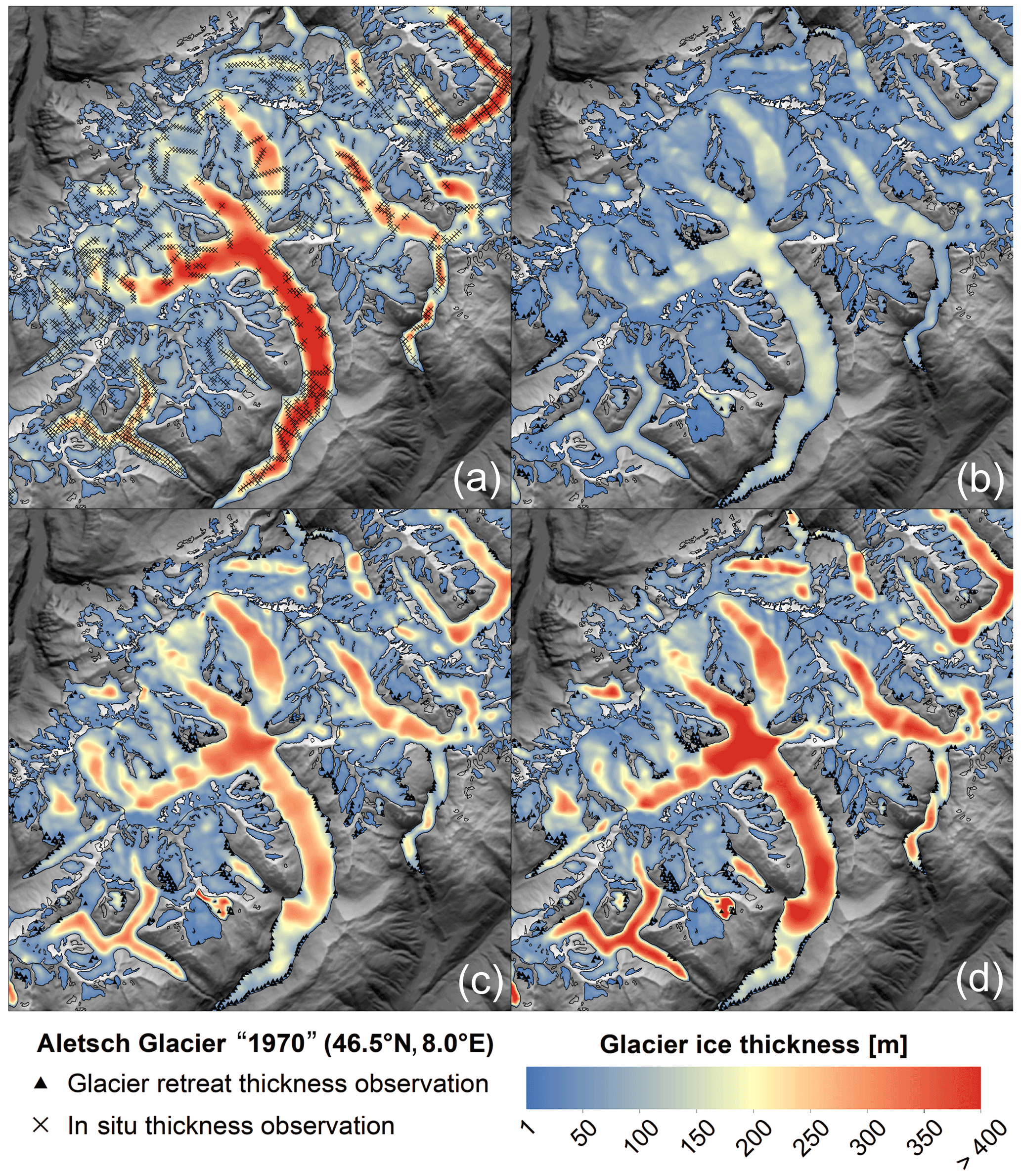
Figure 2 Reconstructed ice thickness of glaciers in the Bernese Alps (Jungfrau-Aletsch) for the 1970s, with the locations of observations from field surveys indicated using black triangles (Grab et al., 2021): (a) glacier thickness estimated from in situ thickness measurements ($H_{\mathrm{SIA}\mathrm{1970}}^{\text{in situ}}$), (b) glacier thickness based on thickness observations (black dots) from glacier retreat areas ($H_{\mathrm{SIA}\mathrm{1970}}^{\mathrm{retreat}\mathrm{01}}$), (c) thickness based on retreat observations and slope-dependent viscosity scaling ($H_{\mathrm{SIA}\mathrm{1970}}^{\mathrm{retreat}\mathrm{02}}$), (d) thickness based on retreat observations and slope- and elevation-dependent viscosity scaling ($H_{\mathrm{SIA}\mathrm{1970}}^{\mathrm{retreat}\mathrm{03}}$).

The second calibration set-up ($H_{\mathrm{SIA}\mathrm{1970}}^{\mathrm{retreat}}$) is exclusively based on thickness observations from glacierized areas that became ice-free between the 1970s and the present ($n_{\mathrm{1970}}^{\mathrm{retreat}}$). Unlike the in situ measurements, the majority of these thickness observations are derived at lower elevations and close to the margin or terminus, as those glacier parts typically show higher retreat rates than the accumulation areas. For the $H_{\mathrm{SIA}\mathrm{1970}}^{\mathrm{retreat}}$ set-up, we perform three iterations of the thickness reconstruction (Figs. 1, 2b–d): (1) without ice viscosity scaling ($H_{\mathrm{SIA}\mathrm{1970}}^{\mathrm{retreat}\mathrm{01}}$), (2) glacier surface slope-based viscosity scaling ($H_{\mathrm{SIA}\mathrm{1970}}^{\mathrm{retreat}\mathrm{02}}$; see Sect. 3.2), and (3) glacier surface elevation- and slope-based viscosity scaling ($H_{\mathrm{SIA}\mathrm{1970}}^{\mathrm{retreat}\mathrm{03}}$; Sect. 3.3). For each iteration of $H_{\mathrm{SIA}\mathrm{1970}}^{\mathrm{retreat}}$, the reconstructed viscosity and thickness are compared to the respective $H_{\mathrm{SIA}\mathrm{1970}}^{\text{in situ}}$ values. The initial iteration ($H_{\mathrm{SIA}\mathrm{1970}}^{\mathrm{retreat}\mathrm{01}}$) includes no additional scaling of the ice viscosity, which is similar to $H_{\mathrm{SIA}\mathrm{1970}}^{\text{in situ}}$. Based on the difference in viscosity between $H_{\mathrm{SIA}\mathrm{1970}}^{\text{in situ}}$ and $H_{\mathrm{SIA}\mathrm{1970}}^{\mathrm{retreat}\mathrm{01}}$ (Sect. 3.2), empirical slope-based scaling factors can be derived that are then applied to the viscosity estimation during the second calibration iteration ($H_{\mathrm{SIA}\mathrm{1970}}^{\mathrm{retreat}\mathrm{02}}$) according to Eq. (5):

$$\begin{array}{}\text{(5)}& {\mathit{\xi }}_{\mathit{\eta }}^{\mathrm{slope}}=y_{\mathit{\eta }}^{\mathrm{slope}}\times \left(\mathit{\alpha }-{\mathit{\alpha }}_{\mathit{\eta }}^{\mathrm{thres}}\right)\text{ for }\mathit{\alpha }\le {\mathit{\alpha }}_{\mathit{\eta }}^{\mathrm{thres}}.\end{array}$$

Here, ${\mathit{\xi }}_{\mathit{\eta }}^{\mathrm{slope}}$ is the slope-based viscosity scaling factor and depends on the local surface slope (α). Calibration parameters are a slope gradient factor ($y_{\mathit{\eta }}^{\mathrm{slope}}$; units per degree) and the respective slope threshold (${\mathit{\alpha }}_{\mathit{\eta }}^{\mathrm{thres}}$) beyond which the viscosity ratio equals one.

Additionally, the slope-based scaling of $H_{\mathrm{SIA}\mathrm{1970}}^{\mathrm{retreat}\mathrm{02}}$ (Fig. 2c) is extended with an elevation-based viscosity scaling ($H_{\mathrm{SIA}\mathrm{1970}}^{\mathrm{retreat}\mathrm{03}}$) to avoid unrealistically high thickness values in the upper-glacier parts. As the vertical extents of Alpine glaciers vary significantly, the elevations of each continuous glacier area are normalized between the lowest (h_min=1) and highest glacier elevation (h_max=0). An additional quantile filter is applied to the elevation range that defines the lowest and highest 2 % of elevation values as one and zero, respectively. By this means, we compensate for uncertainties in the glacier area delineation, as the lowest and highest points of the glacier outline are often difficult to identify due to debris coverage or firn. The second scaling factor is applied based on the linear regression between the ice viscosity and the normalized glacier elevation range (Eq. 6):

$$\begin{array}{}\text{(6)}& {\mathit{\xi }}_{\mathit{\eta }}^{\mathrm{elevation}}=\mathrm{1.0}+y_{\mathit{\eta }}^{\mathrm{elevation}}\times \left(\stackrel{\mathrm{̃}}{h}-{\stackrel{\mathrm{̃}}{h}}_{\mathit{\eta }}^{\mathrm{thres}}\right)\text{ for }\mathrm{0}\le \stackrel{\mathrm{̃}}{h}\le \mathrm{1}.\end{array}$$

Here, ${\mathit{\xi }}_{\mathit{\eta }}^{\mathrm{elevation}}$ is the empirical elevation-range-based correction, which is derived from the normalized local glacier elevation ($\stackrel{\mathrm{̃}}{h}$), the slope of the linear regression ($y_{\mathit{\eta }}^{\mathrm{elevation}}$) and the vertical threshold (${\stackrel{\mathrm{̃}}{h}}_{\mathit{\eta }}^{\mathrm{thres}}$) where no correction is applied. By applying Eq. (6), η is corrected and the final flux field and ice thickness (Fig. 2d) is recalculated considering the slope- and elevation-dependent viscosity ratios ($H_{\mathrm{SIA}\mathrm{1970}}^{\mathrm{retreat}\mathrm{03}}$).

2.5.2 Alps-wide glacier volumes for 2003

For the early 21st century (2003), the glacier volume of all Alpine glaciers ($H_{\mathrm{SIA}\mathrm{2003}}^{\mathrm{retreat}\mathrm{03}}$) is estimated based on RGI glacier areas, the SRTM DEM, and surface elevation changes and mass balance data for the 2000–2014 period. Retreat thickness observations are extracted from glacier areas that have become ice-free since 2000 ($n_{\mathrm{2003}}^{\mathrm{retreat}}$). Additionally, $H_{\mathrm{SIA}\mathrm{2003}}^{\text{in situ}\mathit{\&}\mathrm{retreat}\mathrm{03}}$ is derived from the same input data. However, all available in situ thickness observations ($n_{\mathrm{all}}^{\text{in situ}}$) are integrated as well as observations from glacier areas that have become ice-free since 2000 ($n_{\mathrm{2003}}^{\mathrm{retreat}}$). For both reconstructions, viscosity correction factors are transferred from the estimates of the 1970s Swiss and Austrian glacier volumes (Fig. 1).

3 Results

3.1 The 1970s ice thickness reconstruction and viscosity calibration

3.1.1 In situ thickness reconstruction

The 1970 reference ice thickness ($H_{\mathrm{SIA}\mathrm{1970}}^{\text{in situ}}$) of Swiss and Austrian glaciers is estimated from the historic Swiss and Austrian glacier inventories (SGI1973 and GI1), DEMs (DHM25 and DHM69), and respective surface elevation change and mass balance data. In addition, all $n_{\mathrm{cal}}^{\text{in situ}}$ thickness observations are included to constrain the reconstructed ice thickness distribution. In most cases the survey dates of the in situ measurements differ from the acquisition dates of the DEMs. To derive the respective ice thickness at the acquisition date of the DEM, the in situ observations have to be temporally homogenized. Therefore, we exclusively permit measurements that include both thickness and surface elevation and, thus, provide information on the local basal elevation beneath the glaciers. This is the case for all of the GPR thickness observations (Grab et al., 2021) and almost all of the GlaThiDa entries. For the thickness homogenization and the reconstructions, we assume negligible changes in the basal elevation and subtract it from the reference DEM in 1970 and 2000. The estimated ice volume for the Swiss and Austrian Alps ($V_{\mathrm{SIA}\mathrm{1970}}^{\text{in situ}}$) is 121.6±24.7 km³, corresponding to a glacierized area of 1792.9 km². This is equivalent to 96 % of the total glacier area of the 1973 Swiss and 1969 Austrian inventory.

Table 1 Overview of the experimental set-ups for the 1970 (Swiss and Austrian Alps) and 2003 (entire Alps) reconstruction dates and estimated glacier volumes. $n_{\mathrm{obs}}^{\mathrm{in}\mathrm{situ}}$ and $n_{\mathrm{obs}}^{\mathrm{retreat}}$ indicate the number of thickness measurements from field surveys and DEM differencing used in the respective experimental set-ups. Slope- and elevation-based viscosity scaling factors are given as ${\mathit{\xi }}_{\mathit{\eta }}^{\mathrm{slope}}$ and ${\mathit{\xi }}_{\mathit{\eta }}^{\mathrm{elevation}}$, respectively. Glacier areas refer to ¹ Müller et al. (1976), ² Patzelt (1980) and ³ Paul et al. (2011). The region abbreviations used in the table are as follows: CH – Switzerland, AT – Austria, FR – France and IT – Italy.

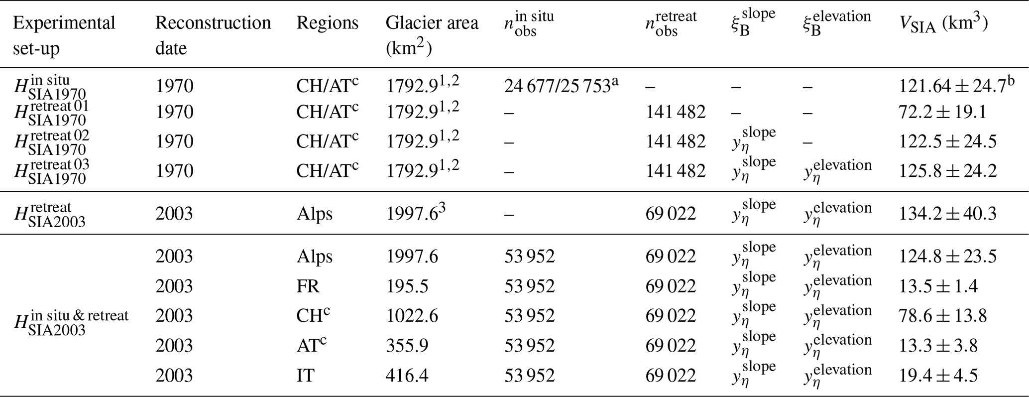
^a Available in situ thickness measurements in the Swiss and Austrian Alps were selected using a 30 m circular buffer and randomly grouped into two subsets. ^b The total volume of glaciers in CH/AT was reconstructed from all available thickness measurements, whereas $y_{\mathit{\eta }}^{\mathrm{slope}}$ and $y_{\mathit{\eta }}^{\mathrm{elevation}}$ were derived from ∼50 % of all in situ thickness measurements. ^c Note that the 1970 and 2003 glacier volumes of the Swiss and Austrian Alps are based on glacier inventories with large differences in glacierized areas due to methodological differences in the delineation and interpretation of glacial extents (see Sect. 4.1).

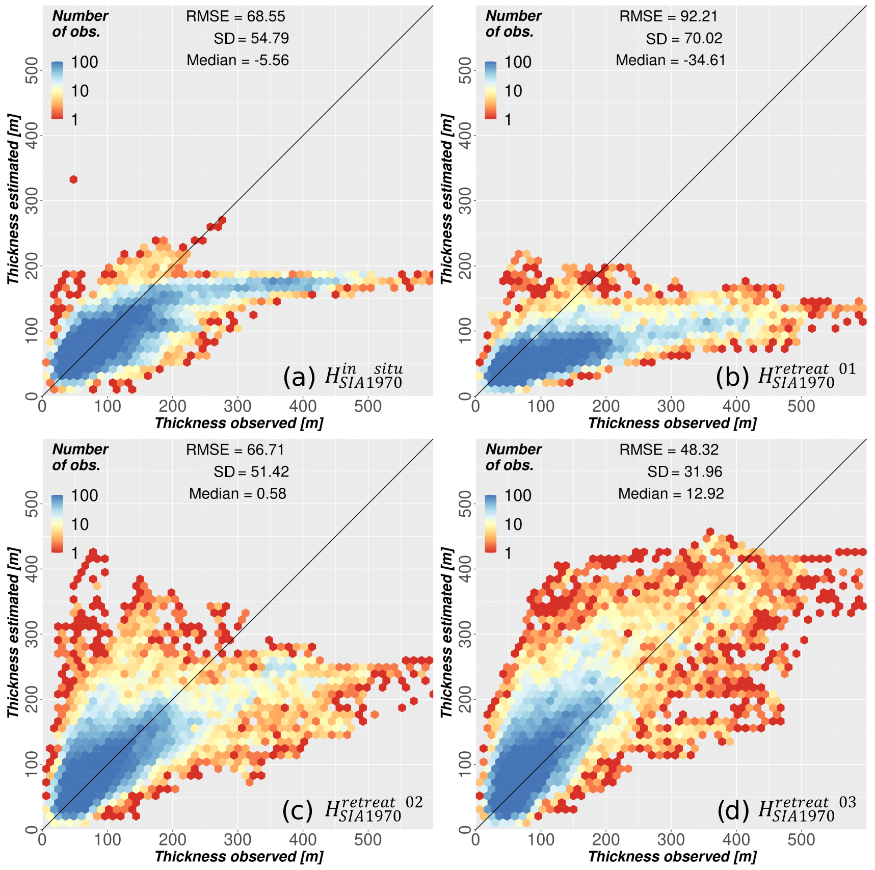
Figure 3 Differences between the estimated ice thickness and observed ice thickness at locations of validation in situ thickness measurements (${\mathrm{n}}_{\mathrm{val}}^{\mathrm{in}\mathrm{situ}}=\mathrm{25}\mathrm{753}$), with the root-mean-square error (RMSE), standard deviation (SD) and median difference (all in metres) given in each panel: (a) reconstruction based on calibration ($n_{\mathrm{cal}}^{\mathrm{in}\mathrm{situ}}$) in situ thickness measurements ($H_{\mathrm{SIA}\mathrm{1970}}^{\mathrm{in}\mathrm{situ}}$), (b) reconstruction based on all glacier thickness observations from deglacierized (retreat) areas ($H_{\mathrm{SIA}\mathrm{1970}}^{\mathrm{retreat}\mathrm{01}}$), (c) reconstruction based on all retreat observations and slope-based viscosity scaling ($H_{\mathrm{SIA}\mathrm{1970}}^{\mathrm{retreat}\mathrm{02}}$), and (d) reconstruction based on all retreat observations and slope- and elevation-based viscosity scaling ($H_{\mathrm{SIA}\mathrm{1970}}^{\mathrm{retreat}\mathrm{03}}$).

3.1.2 Slope-based viscosity scaling

The initial reconstruction of retreat areas ($H_{\mathrm{SIA}\mathrm{1970}}^{\mathrm{retreat}\mathrm{01}}$) is based on the same input data as the reference thickness ($H_{\mathrm{SIA}\mathrm{1970}}^{\text{in situ}}$); however, instead of the in situ observations, thickness values are extracted from deglacierized areas (Sect. 2.4.4). No temporal homogenization of the observations has to be applied, as the ice thickness is directly derived from the state of the reference DEMs. Compared with the $H_{\mathrm{SIA}\mathrm{1970}}^{\text{in situ}}$ reconstruction, the $H_{\mathrm{SIA}\mathrm{1970}}^{\mathrm{retreat}\mathrm{01}}$ underestimates the total glacier volume ($V_{\mathrm{SIA}\mathrm{1970}}^{\mathrm{retreat}\mathrm{01}}$) by approximately 40 % (Table 1) due to a strong negative bias in the estimated ice thickness (Fig. 3b). The largest differences are found at the troughs of large valley glaciers where the observed ice thickness can be twice as high as the reconstructed thickness (Fig. 1). These observations are very similar to the “low elevation bias” configuration used in ITMIX2. The participating models showed large deviations when the available thickness observations were limited to the low and thin glacier parts, where the ice flux is most likely underestimated due to substantial thinning rates and downwasting of the glacier termini (Farinotti et al., 2021).

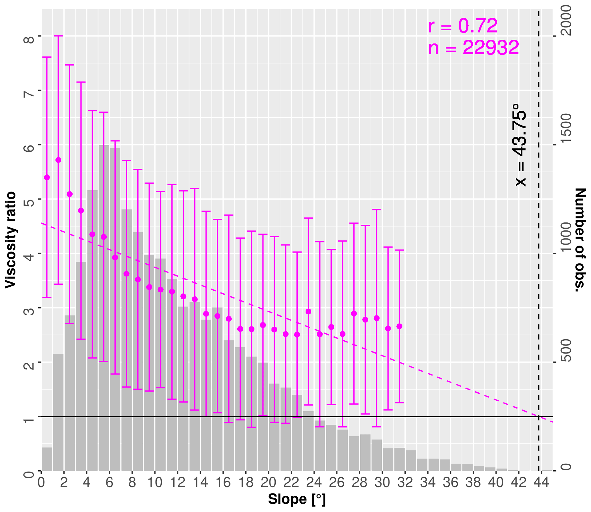
Figure 4 Slope-dependent viscosity ratio of $H_{\mathrm{SIA}\mathrm{1970}}^{\mathrm{in}\mathrm{situ}}$ and $H_{\mathrm{SIA}\mathrm{1970}}^{\mathrm{retreat}\mathrm{01}}$ at the locations of in situ observations. Magenta points denote the mean viscosity ratio values aggregated within 2^∘ slope bins on glacierized areas. The number of observations in each slope bin is shown as grey bars. The respective linear regression of the slope-derived viscosity ratio is shown as a dotted line. Ratios of elevation bins with less than 100 observations are excluded from the analysis. Vertical error bars indicate the respective mean ratio ± 1 standard deviation. The slope threshold (${\mathit{\alpha }}_{\mathit{\eta }}^{\mathrm{thres}}$) is indicated as a vertical black dotted line at 43.75^∘.

To estimate the bias in viscosity between $H_{\mathrm{SIA}\mathrm{1970}}^{\mathrm{retreat}\mathrm{01}}$ and $H_{\mathrm{SIA}\mathrm{1970}}^{\text{in situ}}$, viscosity values are extracted at locations with in situ observations ($n_{\mathrm{cal}}^{\text{in situ}}$) where the ice thickness and viscosity is known. Viscosity values are then aggregated within 2^∘ slope bins to derive the ratio of $H_{\mathrm{SIA}\mathrm{1970}}^{\mathrm{retreat}\mathrm{01}}$ and $H_{\mathrm{SIA}\mathrm{1970}}^{\text{in situ}}$ viscosities (Fig. 4). Average $H_{\mathrm{SIA}\mathrm{1970}}^{\mathrm{retreat}\mathrm{01}}$ viscosities are generally lower than $H_{\mathrm{SIA}\mathrm{1970}}^{\text{in situ}}$, but the difference increases at slopes smaller than 25^∘. Using a linear regression, the slope-scaling parameters of Eq. (5) are $y_{\mathit{\eta }}^{\mathrm{slope}}=-\mathrm{0.08}$ and ${\mathit{\alpha }}_{\mathit{\eta }}^{\mathrm{thres}}=\mathrm{43.75}$^∘. The total ice volume ($V_{\mathrm{SIA}\mathrm{1970}}^{\mathrm{retreat}\mathrm{02}}$) is 122.5±24.5 km³ (Table 1).

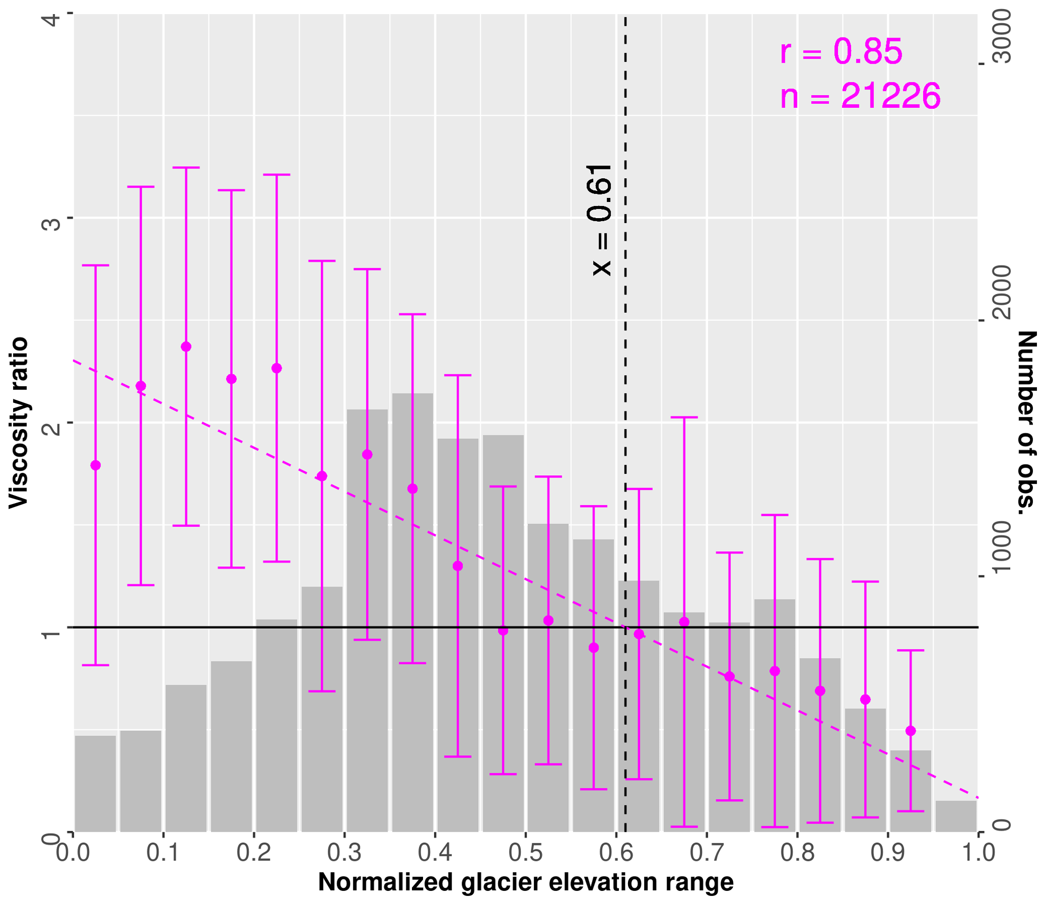
Figure 5 Elevation-dependent viscosity ratio of the $H_{\mathrm{SIA}\mathrm{1970}}^{\mathrm{in}\mathrm{situ}}$ and $H_{\mathrm{SIA}\mathrm{1970}}^{\mathrm{retreat}\mathrm{02}}$ reconstruction at the locations of in situ observations. Elevations have been normalized for each glacier, with 0.0 being the minimum and 1.0 being the maximum glacier height. Magenta points denote the mean viscosity ratio values aggregated within 0.05 normalized elevation bins on glacierized areas. The number of observations in each bin is shown as grey bars. The respective linear regression of the elevation-derived viscosity ratio is shown as a dotted line. Ratios of elevation bins with less than 100 observations are excluded from the analysis. Vertical error bars indicate the respective mean ratio ± 1 standard deviation. The elevation threshold ($h_{\mathit{\eta }}^{\mathrm{thres}}$) is indicated as a vertical black dotted line at a 0.61 normalized glacier elevation.

3.1.3 Elevation-based viscosity scaling

The total ice volume $V_{\mathrm{SIA}\mathrm{1970}}^{\mathrm{retreat}\mathrm{02}}$ is similar to $V_{\mathrm{SIA}\mathrm{1970}}^{\text{in situ}}$. However, the modelled ice thickness tends to overestimate the observed glacier thickness at high altitudes, whereas the lower glacier parts continue to remain too thin (Fig. 2c). The overestimation at high altitudes is likely caused by large firn and ice areas with a small surface slope, where the corrected viscosity is overestimated. Compared with $H_{\mathrm{SIA}\mathrm{1970}}^{\mathrm{retreat}\mathrm{01}}$, the strong negative bias between estimated and observed ice thickness (Fig. 3a) is reduced. Nevertheless, there is a remaining negative offset for glacier parts with an observed ice thickness of more than 300 m (Fig. 3c). Figure 5 shows the mean viscosity ratio of $H_{\mathrm{SIA}\mathrm{1970}}^{\mathrm{retreat}\mathrm{02}}$ and $H_{\mathrm{SIA}\mathrm{1970}}^{\text{in situ}}$ versus the normalized glacier elevation range (Sect. 2.5.1). The ratio of $H_{\mathrm{SIA}\mathrm{1970}}^{\mathrm{retreat}\mathrm{02}}$ to $H_{\mathrm{SIA}\mathrm{1970}}^{\text{in situ}}$ is close to 1 at 0.5–0.6 normalized elevation, which is approximately equal to the glacier median elevation. However, a distinct offset is noticeable at the lowest and highest elevations, where the $H_{\mathrm{SIA}\mathrm{1970}}^{\mathrm{retreat}\mathrm{02}}$ ice viscosity is under- and overestimated, respectively. To compensate for this viscosity biases, $y_{\mathit{\eta }}^{\mathrm{elevation}}=-\mathrm{2.14}$ and $h_{\mathit{\eta }}^{\mathrm{thres}}=\mathrm{0.61}$ are applied based on the linear regression (Eq. 6).

As shown in Fig. 3d, the deviation between observed and estimated ice thickness of thick glacier parts (>300 m ice thickness) further decreases after applying Eq. (6). However, the median difference in $H_{\mathrm{SIA}\mathrm{1970}}^{\mathrm{retreat}\mathrm{03}}$ between observed and estimated ice thickness also increases by ∼10 m compared with $H_{\mathrm{SIA}\mathrm{1970}}^{\mathrm{retreat}\mathrm{02}}$, indicating a slight overestimation of the ice thickness by Eq. (6). The reconstructed total glacier volumes of the different reconstruction steps are shown in Table 1. While there is little difference in the modelled glacier volume of $H_{\mathrm{SIA}\mathrm{1970}}^{\mathrm{retreat}\mathrm{03}}$ and $H_{\mathrm{SIA}\mathrm{1970}}^{\text{in situ}}$ (∼2 %), the inclusion of the elevation-based scaling further improves the spatial thickness distribution (Fig. 2d).

3.2 The 2003 Alps-wide ice thickness reconstruction

${\mathit{\xi }}_{\mathit{\eta }}^{\mathrm{slope}}$ and ${\mathit{\xi }}_{\mathit{\eta }}^{\mathrm{elevation}}$ are transferred to the early 21st century, and the ice thickness of all Alpine glaciers is estimated based on the observation period from 2000 to 2014. The estimated ice volume of $H_{\mathrm{SIA}\mathrm{2003}}^{\text{in situ}\mathit{\&}\mathrm{retreat}}$ is 124.8±23.5 km³. The volume of $H_{\mathrm{SIA}\mathrm{2003}}^{\mathrm{retreat}}$ (134.2±40.3 km³) is relatively similar but ∼7 % higher, mainly due to a likely overestimation of the glacier volume in the Austrian Alps (Table 1).

In the following sections, these reconstructions are used to validate the estimated ice volumes against previous studies on Alpine glacier volumes (Sect. 4.1) and to compare the glacier-specific mean ice thickness of larger Alpine glaciers (Sect. 4.2).

4 Discussion

4.1 Glacier volume comparison

The total 1970 ice volumes of the Swiss and Austrian Alps derived by this study are $H_{\mathrm{1970}}^{\text{in situ}}=\mathrm{121.6}\pm \mathrm{24.7}$ km³ or $H_{\mathrm{1970}}^{\mathrm{retreat}\mathrm{03}}=\mathrm{125.8}\pm \mathrm{24.2}$ km³ (Table 1). For the 1973 Swiss glacier inventory, the estimated volume is $V_{\mathrm{1970}}^{\text{in situ}}=\mathrm{97.7}\pm \mathrm{18.9}$ km³ or $V_{\mathrm{1970}}^{\mathrm{retreat}\mathrm{03}}=\mathrm{99.5}\pm \mathrm{16.9}$ km³. Earlier estimates based on the same glacier area data are available from a number of studies. Müller et al. (1976) and Maisch et al. (2000) reported values of 67 and 74 km³ using empirical relationships between glacier area and mean ice thickness. An ice volume of 75±22 km³ was estimated by Linsbauer et al. (2012) from a subset of glaciers with thickness observations and modelled ice thickness. Based on temporal extrapolation, an ice volume of 94.0±10.9 km³ for the year 1973 was reported (Grab et al., 2021). While the ice volumes of the earlier studies (Müller et al., 1976; Maisch et al., 2000) are substantially lower than our estimate (∼30 %–40 %), good agreement is found with the estimate of the recent study by Grab et al. (2021), supporting their observation of an underestimation of 1970s glacier volumes by older studies using glacier area to volume scaling. With respect to the estimate by Linsbauer et al. (2012), their ice volume is also ∼25 % lower than this study, although the error bars overlap. For the Austrian Alps, our estimated ice volume is $V_{\mathrm{1970}}^{\text{in situ}}=\mathrm{23.9}\pm \mathrm{5.8}$ km³ or $V_{\mathrm{1970}}^{\mathrm{retreat}\mathrm{03}}=\mathrm{25.4}\pm \mathrm{7.3}$ km³ based on the 1969 glacier outlines. A ∼10 % lower ice volume (22.3 km³) for the same year was calculated by Helfricht et al. (2019) from a subset of thickness observations and a calibrated thickness model.

For the entire Alps, our estimated ice volume for the year 2003 is 124.8±23.5 km³ ($H_{\mathrm{SIA}\mathrm{2003}}^{\text{in situ}\mathit{\&}\mathrm{retreat}};H_{\mathrm{SIA}\mathrm{2003}}^{\mathrm{retreat}}=\mathrm{134.2}\pm \mathrm{40.3}$ km³). Glacier volumes for the early 21st century were also reported for the entire Alps (Farinotti et al., 2019a; Millan et al., 2022), the Swiss Alps (Farinotti et al., 2009; Linsbauer et al., 2012; Grab et al., 2021) and the Austrian Alps (Helfricht et al., 2019). An Alps-wide glacier volume of 130±30 km³ was calculated as a consensus estimate from an ensemble of up to five models (Farinotti et al., 2019a), which is close to our estimate. A variant of the reconstruction approach (Fürst et al., 2017) used here also contributed to the consensus estimate. At the time, thickness observations were limited to GlaThiDa v2.01 (Gärtner-Roer et al., 2014; Farinotti et al., 2019a) and, thus, ignored the most recent and comprehensive measurements in Switzerland (Grab et al., 2021). An ice volume of 120±50.0 km³ (2017–2018) for the European Alps and Pyrenees was derived by a recent global study (Millan et al., 2022), based on flow velocity data, which is less than the consensus estimate results and the 2003 glacier volume of this study.

For Swiss glaciers, ice volumes of 74.9±9 km³ (Farinotti et al., 2009), 65±20 km³ (Linsbauer et al., 2012) and 77.2±4.6 km³ (Grab et al., 2021) have been estimated for the beginning of the 21st century. The 2000 Swiss ice volume reconstructed from all available thickness observations ($H_{\mathrm{2003}}^{\text{in situ}\mathit{\&}\mathrm{retreat}}$) in this study is 78.6±13.8 km³, which is ∼20 % higher than the estimate by Linsbauer et al. (2012) but close to the glacier volume by Farinotti et al. (2009) and Grab et al. (2021). Nevertheless, the error bars of all estimates overlap. Regarding glaciers of the Austrian Alps, the estimated ice volume of 13.3±3.8 km³ (2003) is lower than the value by Helfricht et al. (2019) for the year 1998 (19.7 km³). It is noteworthy that the glacierized areas of the estimates by Farinotti et al. (2009), Linsbauer et al. (2012), Helfricht et al. (2019), Grab et al. (2021) and this study vary, as the aforementioned studies used the respective regional glacier inventories for the Swiss and Austrian Alps. Differences in the delineation of glacier areas arise from the applied datasets and the interpretation of glacier areas. Particularly for the Austrian Alps, large differences in regional glacier extents can be observed between the RGI glacier areas used in this study (Paul et al., 2011) and the Austrian glacier inventories GI2 and GI3 (Lambrecht and Kuhn, 2007; Fischer et al., 2015b). Spatial differences in the delineation of glacier outlines appear to be mostly connected to small- and medium-sized glaciers and might be, at least partially, explained by the integration of perennial snowfields in the Austrian inventories, as described by previous studies (Lambrecht and Kuhn, 2007; Paul et al., 2011). Therefore, a direct comparison of the GI2 and RGI glacier areas is difficult as reported by previous studies (Paul et al., 2011; Fischer et al., 2015b). In addition, the RGI glacier area attributed to the Austrian Alps by this study is further reduced, as we masked all glacierized areas to the Austrian country border in order to derive the specific glacier volumes of each Alpine country (Table 1). We assume that the large differences in glacier volume for the early 21st century between this study and Helfricht et al. (2019) are related to the substantial differences in the glacier area in the inventories used.

Assessing the difference in Austrian glacier volumes for 1969 between this work and a previous study (Helfricht et al., 2019) is more complex, as both studies are based on the same glacier inventory. Between 1969 and 1998, a volume change of −4.9 km³ was measured by Lambrecht and Kuhn (2007) based on DEM differencing. For the very similar observation period from 1969 to 2000, we derive a volume change rate of $-\mathrm{0.21}\pm \mathrm{0.04}$ km³ a⁻¹ from the input DEMs (SRTM − DHM69) used in this study (Sect. 2.4.1); this results in a more negative total volume change of $-\mathrm{6.0}\pm \mathrm{1.1}$ km³ for the reference period from 1969 to 1998, which might be related to a negative elevation bias in the SRTM DEM at high altitudes (e.g. Berthier et al., 2006). Therefore, a potential explanation for the higher 1969 glacier volume in this study might be an overestimation of the surface elevation changes, and thus mass loss, of Austrian glaciers since 1969.

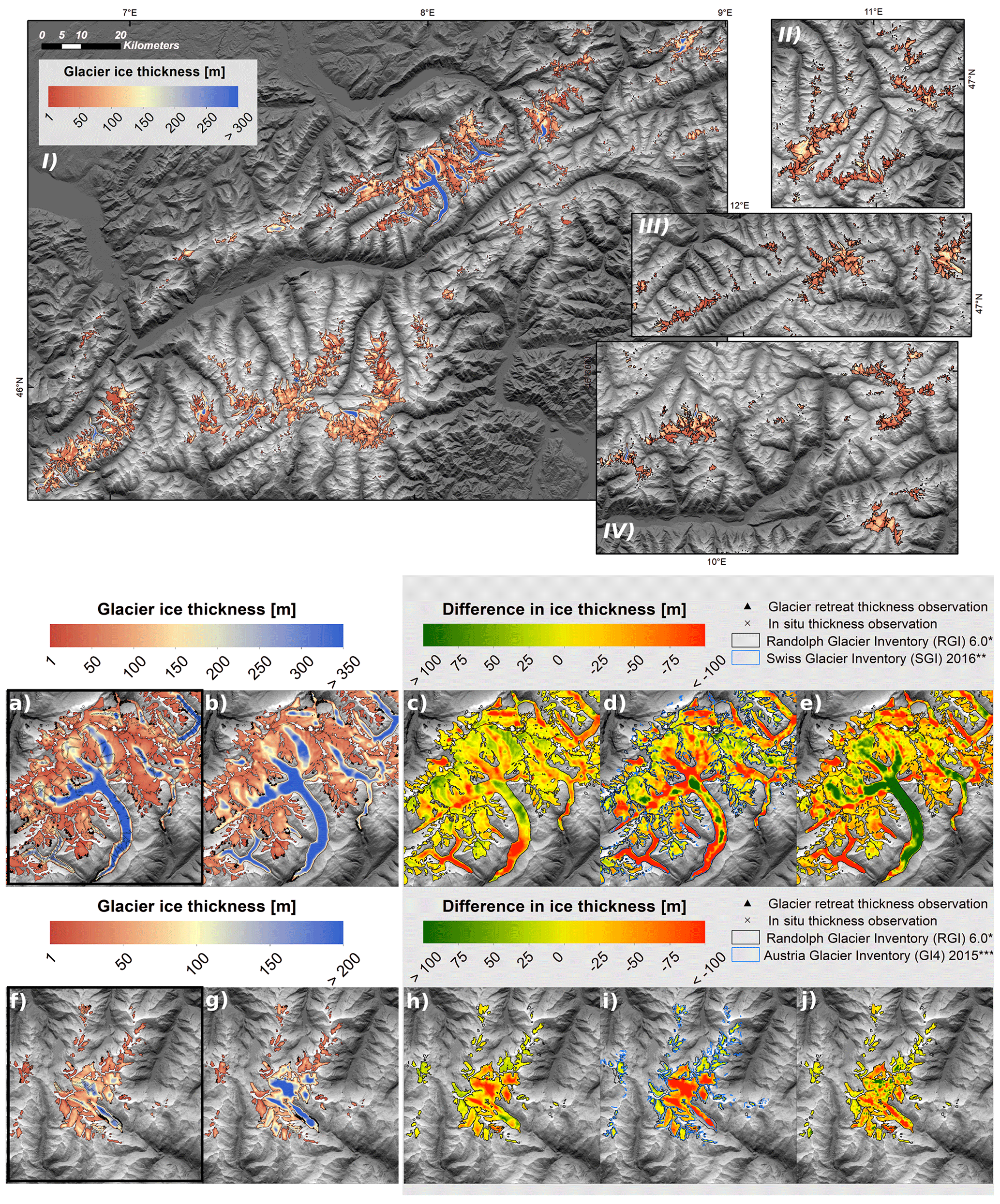
Figure 6 Reconstructed ice thickness ($H_{\mathrm{SIA}\mathrm{2003}}^{\text{in situ}\mathit{\&}\mathrm{retreat}}$) of glaciers in the European Alps (2003): (I) Mont Blanc Group, Pennine and Bernese Alps; (II) Ötztal and Stubai Alps; (III) Zillertal Alps, Venediger and Glockner Group; (IV) Silvretta Alps; and comparison of the ice thickness distribution of Aletsch (CH) (a–e) and Pasterze Glacier (AT) (f–j) by this study and previously published reference ice thickness maps. Panels (a) and (f) and panels (b) and (g) show the distributed glacier thickness as estimated by the $H_{\mathrm{SIA}\mathrm{2003}}^{\text{in situ}\mathit{\&}\mathrm{retreat}}$ and $H_{\mathrm{SIA}\mathrm{2003}}^{\mathrm{retreat}}$ reconstructions, respectively, while panels (c), (d) and (e) and panels (h), (i) and (j) indicate vertical differences in reconstructed ice thickness between $H_{\mathrm{SIA}\mathrm{2003}}^{\mathrm{retreat}}$ (b, g) and Farinotti et al. (2019a) (c, h), Grab et al. (2021) (d), Helfricht et al. (2019) (i) and Millan et al. (2022) (e, j). The ice thickness maps by Farinotti et al. (2019a) refer to the results of the multi-model ensemble of ITMIX. The modelled ice thickness of Grosser Aletsch (Grab et al., 2021) and Pasterze Glacier (Helfricht et al., 2019) are constrained by in situ measurements. Millan et al. (2022) uses glacier flow velocities from remote-sensing data to derive the ice thickness distribution. (The background map is SRTM hillshade.)

4.2 Reconstructed ice thickness distribution

To evaluate the ice thickness distribution of the $H_{\mathrm{SIA}\mathrm{2003}}^{\mathrm{retreat}}$ reconstruction, the estimated ice thickness maps are directly compared to previous reconstructions of the 21st century glacier volume of the European Alps.

A comparison of previous ice thickness reconstructions based on different reconstruction approaches (Farinotti et al., 2019a; Helfricht et al., 2019; Grab et al., 2021; Millan et al., 2022) is shown in Figs. 6 and S3 for Grosser Aletsch (Fig. 6a–e) and Pasterze (Fig. 6f–j) glaciers. While the $H_{\mathrm{SIA}\mathrm{2003}}^{\text{in situ}\mathit{\&}\mathrm{retreat}}$ ice thickness maps are relatively similar to the other in situ observation-based reconstructions, the estimated ice volume of the $H_{\mathrm{SIA}\mathrm{2003}}^{\mathrm{retreat}}$ reconstruction is spread more evenly across the entire glacier domain, i.e. there is a tendency to overestimate or underestimate the thickness of thin and thick glacier parts, respectively. This is particularly noticeable in the upper areas of the Grosser Aletsch (Fig. 6b). Occasionally, we find spuriously large values in certain confined areas, such as in the upper part of Pasterze Glacier (Fig. 6g). In contrast, glacier parts with very high ice thickness are often underestimated by the $H_{\mathrm{SIA}\mathrm{2003}}^{\mathrm{retreat}}$ reconstruction, such as Konkordiaplatz (Concordia Place) for the Grosser Aletsch (Fig. 6b).

Figure 7 Mean ice thickness of large Alpine glaciers (>10 km²) estimated by this study and previous reconstructions (Farinotti et al., 2019a; Helfricht et al., 2019; Grab et al., 2021; Millan et al., 2022). Red dots and brown triangles indicate the mean $H_{\mathrm{SIA}\mathrm{2003}}^{\text{in situ}\mathit{\&}\mathrm{retreat}}$ and $H_{\mathrm{SIA}\mathrm{2003}}^{\mathrm{retreat}}$ glacier thickness of this study, respectively. The reconstructions by Helfricht et al. (2019), Grab et al. (2021) and Millan et al. (2022) refer to the years 2006, 2016 and 2017–2018, respectively. Therefore, hollow symbols represent the original mean value derived from the published ice thickness maps, and filled symbols show the mean glacier thickness temporally extrapolated to the year 2000. * For glaciers without in situ observations, only the $H_{\mathrm{SIA}\mathrm{2003}}^{\mathrm{retreat}}$ reconstruction is shown.

For a direct assessment of glacier-specific mean ice thickness, we refer to a comparison between published ice thickness maps of prominent Alpine glaciers (Farinotti et al., 2019a; Helfricht et al., 2019; Grab et al., 2021; Millan et al., 2022) and this study (Fig. 7). For the comparison of mean glacier thicknesses, we use the respective glacier elevation change rates (Sect. 2.4.2) to reduce temporal differences between the datasets. The reason is that previous glacier thickness maps refer to the years 2016–2018 (Grab et al., 2021; Millan et al., 2022) and 2006 (Helfricht et al., 2019). Nevertheless, both values (the originally published and temporally extrapolated mean ice thickness of each study) are shown in Fig. 7. In general, the mean $H_{\mathrm{SIA}\mathrm{2003}}^{\text{in situ}\mathit{\&}\mathrm{retreat}}$ and $H_{\mathrm{SIA}\mathrm{2003}}^{\mathrm{retreat}}$ ice thickness of most glaciers is similar to previously reported values. However, in some cases, the $H_{\mathrm{SIA}\mathrm{2003}}^{\mathrm{retreat}}$ reconstruction deviates more from the mean glacier thickness found by other studies. Particularly for the Adamello and Trift glaciers, the mean ice thickness of the $H_{\mathrm{SIA}\mathrm{2003}}^{\mathrm{retreat}}$ reconstruction is substantially lower or higher.

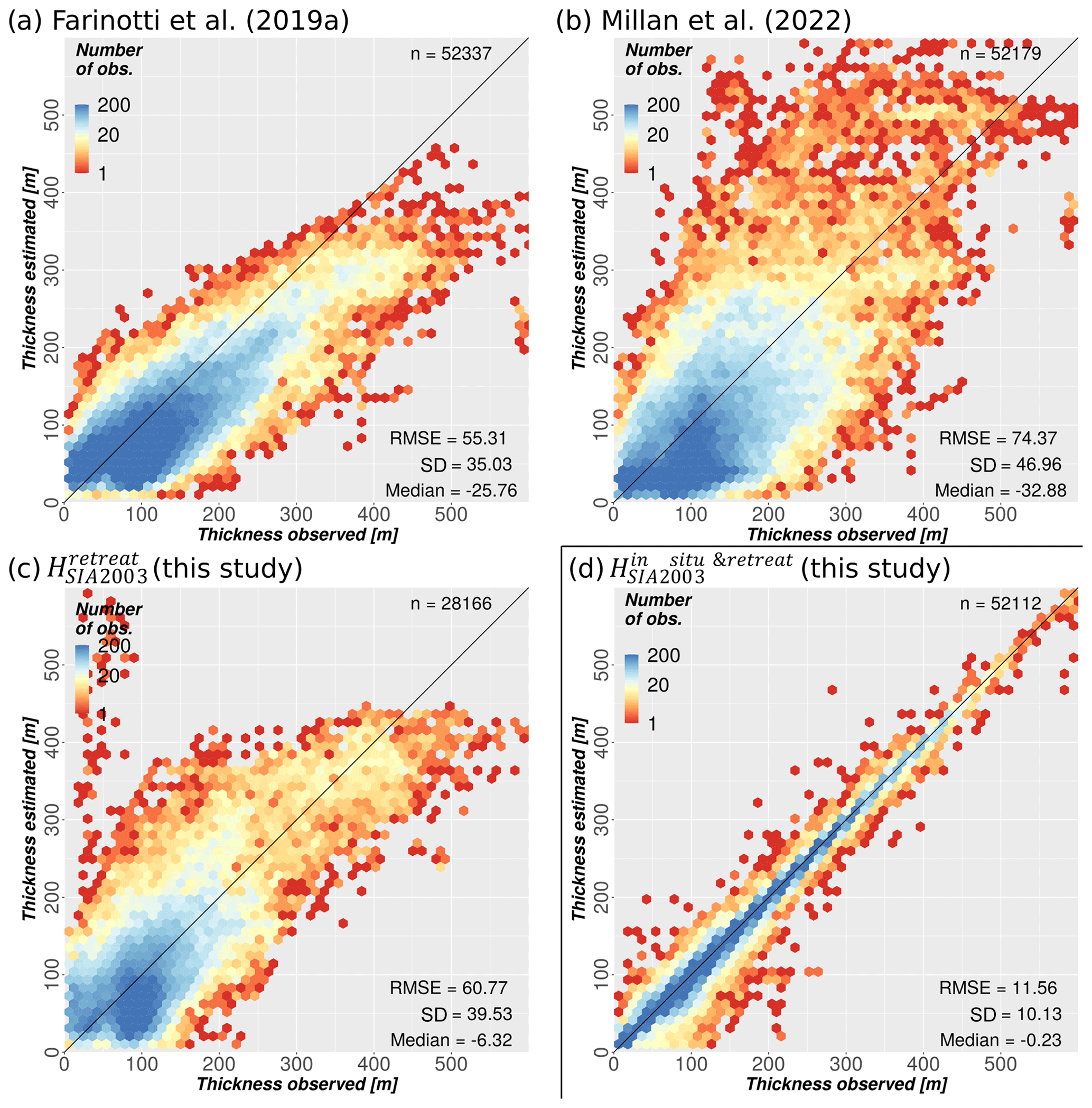
Figure 8 Difference between in situ observations and estimated (2000) local ice thickness, with the root-mean-square error (RMSE), standard deviation (SD) and median difference (all in metres) given in each panel. Panels (a) and (b) refer to published ice thickness maps by Farinotti et al. (2019a) and Millan et al. (2022). Differences between estimated and observed ice thickness are derived from all available in situ measurements (GlaThiDa; Grab et al., 2021). Deviations in ice thickness in the $H_{\mathrm{SIA}\mathrm{2003}}^{\mathrm{retreat}}$ reconstruction of this study are shown in panel (c). Note that the in situ observations from glaciers used to derive the viscosity scaling factors (Sect. 2.5) are excluded from the comparison. Panel (d) indicates the ice thickness distribution based on all available in situ and retreat observations as well as the viscosity scaling factors ($H_{\mathrm{SIA}\mathrm{2003}}^{\text{in situ}\mathit{\&}\mathrm{retreat}}$). Note the logarithmic scaling of the thickness observations' distribution. Dark blue areas indicate hexbins with more than 200 thickness measurement locations.

Point-specific offsets between in situ measurements of ice thickness and reconstructed glacier thickness are shown in Fig. 8. Figure 8a and b refer to previously published Alps-wide ice thickness maps (Farinotti et al., 2019; Millan et al., 2022). Differences between estimated and observed ice thickness in Fig. 8a and b are derived from all in situ observations (GlaThiDa; Grab et al., 2021). For $H_{\mathrm{SIA}\mathrm{2003}}^{\mathrm{retreat}}$, it should be noted that differences are only computed on glaciers for which thickness measurements were ignored in the calibration (Fig. 8c). These first three approaches have all been regionally calibrated in the Alps and do not necessarily reproduce local thickness observations. In this sense, a direct comparison is reasonable. The respective root-mean-square error (RMSE) values of local thickness are 55 and 74 m for the datasets by Farinotti et al. (2019a) and Millan et al. (2022), with both studies indicating a general underestimation (26 and 33 m median deviation, respectively). Thickness differences in the $H_{\mathrm{SIA}\mathrm{2003}}^{\mathrm{retreat}}$ reconstruction indicate no obvious trend with respect to an over- or underestimation of ice thickness for most glacier parts, and the median difference is significantly reduced with respect to the previous reconstructions. Concerning the standard deviation, the $H_{\mathrm{SIA}\mathrm{2003}}^{\mathrm{retreat}}$ results are similar to both Farinotti et al. (2019a) and Millan et al. (2022).

Additionally, the ability of the applied reconstruction to reproduce available thickness observations is demonstrated in Fig. 8d. The underlying model by Fürst et al. (2017) is specifically constructed with a focus on the integration and reproduction of observed ice thicknesses. In this context, there are no indications of a systematic bias in ice thickness, introduced by the viscosity scaling approach and the retreat observations. Remaining deviations of about 10 m are likely associated with a posteriori interpolation of the thickness map to the measurement locations, which is required for this comparison.

In summary, the $H_{\mathrm{SIA}\mathrm{2003}}^{\mathrm{retreat}}$ ice thickness distribution appears to be smoother than reconstructions including in situ measurements ($H_{\mathrm{SIA}\mathrm{2003}}^{\text{in situ}\mathit{\&}\mathrm{retreat}}$). This implies larger local uncertainties. To a certain degree, this has to be expected, as the ice thickness of the inner glacier parts is naturally better constrained if respective field surveys are available. For the viscosity-scaling-based reconstruction, in contrast, the ice thickness of the inner glacier parts is widely unknown and has to be estimated exclusively from the viscosity correction parameters. Depending on the specific glacier morphology, this can result in large local uncertainties (Figs. 6, 7). Particularly, topographic characteristics of the glacier bedrock, such as overdeepenings or cirque thresholds, are challenging to reproduce when there are no direct observations of the thick glacier parts.

4.3 Uncertainty in the viscosity scaling and retreat thickness

Similar to the findings of ITMIX2, a substantial underestimation of the glacier volume was found when relying solely on thickness observations from the lower and thin glacier parts. The presented viscosity scaling approach reproduces the region-wide glacier volume and thickness distribution well, yet there are larger uncertainties in the glacier-specific ice thickness distribution.

Assuming the SIA, the ice thickness is derived from the glacier-wide flux field (Eq. 3), whereas the ice viscosity is initially unknown. The viscosity is estimated at locations with thickness observations and subsequently interpolated across the entire glacier domain. For the $H_{\mathrm{SIA}\mathrm{1970}}^{\mathrm{retreat}}$ reconstructions, the interpolated viscosity field is generally lower than the $H_{\mathrm{SIA}\mathrm{1970}}^{\text{in situ}}$ viscosity field, as the observations used exclusively represent the relatively thin glacier margins with low viscosity values. Conversely, the $H_{\mathrm{SIA}\mathrm{1970}}^{\text{in situ}}$ viscosity distribution is derived from thickness observations of the inner glacier parts with higher viscosity values, resulting in an overall higher ice thickness. To account for this generic limitation of the glacier-margin-based viscosity interpolation, the $H_{\mathrm{SIA}\mathrm{1970}}^{\mathrm{retreat}}$ ice viscosities have to be corrected before the final ice flux is calculated.

The initial slope-dependent viscosity correction (${\mathit{\xi }}_{\mathit{\eta }}^{\mathrm{slope}}$) shows a tendency to overestimate the ice thickness at high elevations. This pattern can be directly observed in the ice thickness maps (Figs. 5, 6). This is likely caused by the relatively large and flat accumulation areas of some Alpine glaciers where a high correction factor is applied to the ice flux. A very prominent example of such a significant overestimation of the actual ice thickness by the $H_{\mathrm{SIA}\mathrm{2003}}^{\mathrm{retreat}}$ reconstruction can be observed at the Pasterze Glacier in Fig. 6f and g. For the large and mostly flat upper part of Pasterze Glacier, high viscosity values are estimated by the regionally calibrated slope-dependent correction. Without direct thickness measurements, it is very difficult to avoid these local biases. To compensate for this overestimation of ice thickness, the additional elevation-dependent scaling (${\mathit{\xi }}_{\mathit{\eta }}^{\mathrm{elevation}}$) reduces the correction factor in the upper-glacier parts and vice versa. However, the ${\mathit{\xi }}_{\mathit{\eta }}^{\mathrm{elevation}}$ correction, which is based on the normalized glacier elevation range, can be biased when applied to large consecutive glacier areas. For instance, in the case of the Jungfrau-Aletsch Glacier area (Fig. 1), the ice flux correction of the smaller glaciers is biased by the asymmetric distribution of the vertical extents of the individual glaciers. While the overall elevation range of this consecutive glacier area is determined by the terminus and high-firn areas of the Grosser Aletsch, the adjacent glaciers (e.g. Oberaletschgletscher) have a much smaller vertical extent. This can result in rather high or low ${\mathit{\xi }}_{\mathit{\eta }}^{\mathrm{elevation}}$ correction factors depending on the vertical extent of the glacier in relation to the entire glacierized area. Another source of uncertainty can be an indeterminate separation between glacier ice and perennial snow, as frequently found at high altitudes. In those cases, high thickness values are modelled on adjacent snow areas with small slopes, and the normalized elevation range, which is used for the second correction step, can be shifted upwards, resulting in rather thick accumulation areas.

In addition, it should be noted that the derived retreat thickness observations can be somewhat biased by terrain elevation changes in the glacier foreland, such as erosion and sedimentation, after the deglaciation. To reduce potential biases due to “unstable” height change measurements on glacier retreat areas, we exclude observations that are close (<30 m) to either the past or present glacier outline and apply a slope threshold (25^∘). However, based on the available DEM differences, it is not possible to differentiate between height changes prior to or after the deglaciation of the glacier foreland. Therefore, we cannot completely avoid uncertainties in the extracted retreat thickness due to geomorphological processes.

All in all, the glacier-specific accuracy of the correction parameters and retreat thickness information can be somewhat influenced by the quality of the glacier inventory or the geometries of nearby glaciers. The approach is most favourable in cases where no or only a small sample of direct thickness observations is available. With the increasing number of satellite remote-sensing data, the accuracy of the estimated ice thickness distribution can be improved by new high-resolution glacier inventories or elevation change measurements. Eventually, the presented approach could be most beneficial in regions with large glacierized areas and sparse thickness observations, as the glacier volume has to be inferred mostly from remote-sensing information. However, another potential source of uncertainty, regarding the transferability of the presented correction terms to glacierized areas outside the European Alps, results from the varying regional glacier morphologies in terms of size composition and elevation range. While the empirical relations found between ice viscosity and glacier surface topography have been applied to a different observation period and larger study region ($H_{\mathrm{SIA}\mathrm{2003}}^{\mathrm{retreat}}$), we expect that the scaling functions are, to some degree, related to the geometries and size distribution of glaciers in the Swiss and Austrian Alps. In the European Alps, this uncertainty cannot be avoided, as the overall distribution of a large number of small- to medium-sized cirque glaciers with few large valley glaciers remains unchanged between $H_{\mathrm{SIA}\mathrm{1970}}^{\mathrm{retreat}}$ and $H_{\mathrm{SIA}\mathrm{2003}}^{\mathrm{retreat}}$, despite the substantial reduction in glacierized area since the 1970s. Furthermore, the presented relations might be linked to the geographic environment of the European Alps, as glacier changes are connected to the surrounding topography and climatic conditions (Abermann et al., 2011). To quantify these relations between the Alpine topography, glacier geometries and the derived scaling parameters and to examine the transferability, it would be mandatory to extend the presented analysis to another glacierized region with different glacier morphology, such as marine- and lake-terminating glaciers, as well as different climatic settings, which is beyond the scope of this work.

5 Conclusions

We present a topography-based scaling approach to estimate region-wide glacier volumes from retreat thickness observations derived from remote-sensing acquisitions. The method is based on an empirical relationship between in situ observations and modelled ice thickness distributions of Alpine glaciers. Firstly, a slope-dependent correction is applied to compensate for a general bias in the estimated ice volume due to the spatial distribution of retreat thickness observations. Secondly, an elevation-based correction is required to constrain the ice thickness distribution over the vertical glacier extent. It is shown that the applied viscosity corrections are able to provide a robust estimation of region-wide glacier volumes. Moreover, the empirical scaling relations improve the distribution of the ice thickness over the drainage basin. Compared with previous reconstructions and in situ measurements of ice thickness, the median deviation between observed and modelled glacier thickness is significantly reduced (−6.3 m), whereas the root-mean-square error (60.8 m) and standard deviation (39.5 m) are similar. However, we still notice a tendency for thickness underestimation along the lower trunks and an overestimation at high altitudes where the topography is gently sloping.

We provide additional ice thickness maps for 1970 (Swiss and Austrian Alps) and 2003 (Alps) that are derived from all available in situ thickness measurements and retreat thickness values from DEM differencing. The hereby reconstructed ice volume of the 21st century for the RGI version 6 glacier area is 126.1±23.5 km³ (2003) for the entire Alps. For glaciers of the Swiss and Austrian Alps, the ice volume was 121.6±24.7 km³ in 1970 based on glacierized areas of the SGI1973 and GI1.

The reconstruction approach shown in this study has the potential to constrain estimates of the ice thickness distribution in regions without direct observations of glacier thickness. Nevertheless, there is still room for improvement with respect to the spatial distribution of estimated ice thicknesses. Particularly, the second elevation-based viscosity correction does not completely compensate for hypsometric biases in local ice thickness distribution in the case of certain glacier geometries. Furthermore, while the extraction of retreat ice thickness information from deglacierized areas is relatively straightforward in most mountain regions, the transferability of the viscosity scaling factors derived from Alpine glaciers to other unsurveyed mountain regions needs to be assessed. Therefore, future work will have to address the applicability of the presented approach in regions with different glacier geometries and climatic settings, such as the South American Andes or High Mountain Asia.