the Creative Commons Attribution 4.0 License.
the Creative Commons Attribution 4.0 License.
 | 23 May 2023
Representation of soil hydrology in permafrost regions may explain large part of inter-model spread in simulated Arctic and subarctic climate
Philipp de Vrese
Goran Georgievski
Jesus Fidel Gonzalez Rouco
Dirk Notz
Tobias Stacke
Norman Julius Steinert
Stiig Wilkenskjeld
Victor Brovkin
The current generation of Earth system models exhibits large inter-model differences in the simulated climate of the Arctic and subarctic zone, with differences in model structure and parametrizations being one of the main sources of uncertainty. One particularly challenging aspect in modelling is the representation of terrestrial processes in permafrost-affected regions, which are often governed by spatial heterogeneity far below the resolution of the models' land surface components. Here, we use the Max Planck Institute (MPI) Earth System Model to investigate how different plausible assumptions for the representation of permafrost hydrology modulate land–atmosphere interactions and how the resulting feedbacks affect not only the regional and global climate, but also our ability to predict whether the high latitudes will become wetter or drier in a warmer future. Focusing on two idealized setups that induce comparatively “wet” or “dry” conditions in regions that are presently affected by permafrost, we find that the parameter settings determine the direction of the 21st-century trend in the simulated soil water content and result in substantial differences in the land–atmosphere exchange of energy and moisture. The latter leads to differences in the simulated cloud cover during spring and summer and thus in the planetary energy uptake. The respective effects are so pronounced that uncertainties in the representation of the Arctic hydrological cycle can help to explain a large fraction of the inter-model spread in regional surface temperatures and precipitation. Furthermore, they affect a range of components of the Earth system as far to the south as the tropics. With both setups being similarly plausible, our findings highlight the need for more observational constraints on the permafrost hydrology to reduce the inter-model spread in Arctic climate projections.
- Article
(7250 KB) - Full-text XML
-
Supplement
(30544 KB) - BibTeX
- EndNote


Earth system models (ESMs) are our primary tool for projecting the coupled dynamics of the climate and biogeochemistry under future emission scenarios (Flato, 2011; Stocker et al., 2013), with the ensemble of simulations from the Coupled Model Intercomparison Project (CMIP; Taylor et al., 2012; Eyring et al., 2016) providing an important basis for policy-making (IPCC, 2021). But while ESMs agree on the general relation between increasing greenhouse gas concentrations and rising temperatures, there are substantial differences between the climate states and trajectories simulated by individual models. These inter-model differences are particularly prominent in the northern high latitudes, where ESMs estimate very different sea-ice concentrations (Notz and SIMIP Community, 2020; Davy and Outten, 2020) as well as different surface temperatures and evapotranspiration and precipitation rates (Fig. 1). The region is of special interest not only because polar amplification causes temperatures there to increase at least twice as fast as the global average (Brown and Romanovsky, 2008; Stocker et al., 2013; Biskaborn et al., 2019), but also because Arctic and subarctic soils contain roughly 1100–1700 Gt of carbon, which is about twice as much as is contained in Earth's atmosphere (Zimov et al., 2006; Schirrmeister et al., 2011; Strauss et al., 2015; Bernal et al., 2016; Vasilchuk and Vasilchuk, 2017; Tarnocai et al., 2009; Hugelius et al., 2013, 2014). Currently, the majority of these soil carbon pools are effectively inert as they are contained within permafrost – perennially frozen ground – but more and more of the organic matter will become vulnerable to decomposition as a consequence of global warming. The resulting CO2 and CH4 emissions further increase the rise in temperatures, making the permafrost carbon feedback an important but highly uncertain terrestrial climate feedback (Zimov et al., 2006; Schaefer et al., 2014; MacDougall et al., 2015; Schuur et al., 2015; Comyn-Platt et al., 2018; Gasser et al., 2018; Lenton et al., 2019; Randers and Goluke, 2020; Turetsky et al., 2020; de Vrese et al., 2021; Natali et al., 2021).

Figure 1CMIP6 ensemble spread and permafrost regions: standard deviation (σ) of the CMIP6 model ensemble averaged for the period 1980–2000 – (a) evapotranspiration, (b) precipitation and (c) surface temperatures. Plots are based on 44 simulations provided by 27 modelling groups (see Table S2). (d) Northern mid- and high-latitude permafrost regions.
Studies have identified differences in model structure and parametrizations as one of the main sources of uncertainty in Arctic climate change projections (Hodson et al., 2012; Lehner et al., 2020; Bonan et al., 2021), but it is difficult to attribute the inter-model climate variability to differences in specific model components. With respect to the land surface, it appears likely that the treatment of snow is a main contributor to the model uncertainty. The high-latitude snow cover lasts for the majority of the year, and differences in the simulated snowpack have been shown to often coincide with large differences in surface and subsurface temperatures (Paquin and Sushama, 2014; Ekici et al., 2015; Melo-Aguilar et al., 2018; Mudryk et al., 2020; Menard et al., 2021). During the snow-free season, the land–atmosphere exchange of energy, moisture and momentum is determined by a number of soil and vegetation properties, all of which depend – directly or indirectly – on the representation of the terrestrial hydrology (Seneviratne et al., 2010). The partitioning of the net radiation into latent and sensible heat flux, which is a key factor in the development of the near-surface temperatures, cloud formation and precipitation, depends on the amount of water that can be evaporated and transpired. The albedo of bare ground is influenced by the soil wetness at the surface, while the extent of these bare areas is partly determined by the root-zone soil moisture as an important factor for the vegetation cover. The latter also determines the surface albedo in vegetated areas and affects the exchange of momentum via its effect on the surface roughness. Thus, with almost every aspect of land–atmosphere interactions being affected by the availability of liquid water, it is plausible that the representation of the soil hydrology in numerical models is a major contributor to inter-model climate variability.
Representing the soil hydrology of the Arctic and subarctic zone with coarse-resolution land surface models (LSMs) is especially challenging because the hydrology is often determined by small-scale landscape heterogeneity and affected by processes that are spatially and temporarily very confined. Prominent examples are the spatial soil moisture variability of the polygonal tundra (Cresto Aleina et al., 2013) and geomorphological processes linked to soil ice, including thermokarst features, thaw lake dynamics and ground subsidence (Jorgenson et al., 2006; O'Donnell et al., 2011; Liljedahl et al., 2016; Serreze et al., 2000; Jafarov et al., 2018; Nitzbon et al., 2019; Andresen and Lougheed, 2015). Permafrost plays a key role in the terrestrial hydrological cycle because the presence of ice modulates the thermophysical soil properties as well as infiltration rates and the vertical and lateral movement of water through the ground. And while LSMs will never be able to capture the full multitude of effects connected to surface and subsurface heterogeneity, the level of realism in the representation of physical and biogeochemical permafrost-related processes and effects has increased substantially over the past years (McGuire et al., 2016; Chadburn et al., 2017; Fisher and Koven, 2020; Blyth et al., 2021). Amongst other aspects, many models now account for the inhibition of vertical soil moisture fluxes, which often leads to the formation of a saturated zone above the permafrost table, or the thermal insulation of the soil due to organic matter (Painter et al., 2012; Swenson et al., 2012; Toride et al., 2013; Walvoord and Kurylyk, 2016).
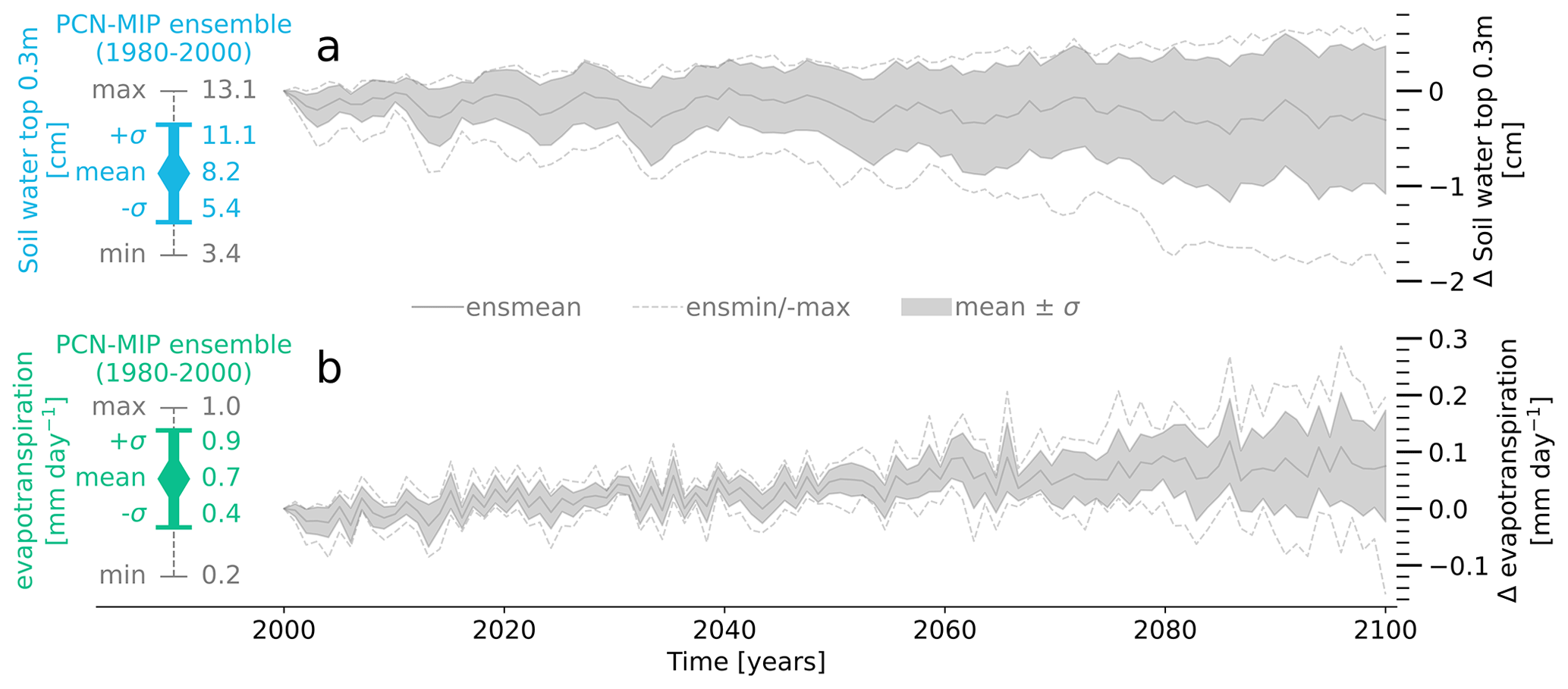
Figure 2PCN-MIP: (a) simulated soil water content in the top 30 cm of the soil averaged across the northern permafrost regions. Shown are the minimum, the mean (± 1 standard deviation; σ) and the maximum of the ensemble of Permafrost Carbon Network Model Intercomparison Project (PCN-MIP; McGuire et al., 2018) participants. The left side shows the 1980–2000 mean and the right side the changes during the 21st century (relative to the 1980–2000 mean). (b) Same as (a) but for evapotranspiration. The figure is based on Andresen et al. (2020), but the analysis was slightly modified in that we aggregated the output of all models over the permafrost regions shown in Fig. 1d, instead of the initial permafrost domain as simulated by the individual models. Furthermore, we included a simulation with the JSBACH model in the intercomparison.
These model developments help improve our understanding of the ways permafrost affects the regional climate and the terrestrial carbon cycle. Still, it remains unclear how differences in the treatment of the soil hydrology in permafrost regions relate to the inter-model climate variability in the present generation of ESMs. In part, this is because it is next to impossible to determine whether differences in Arctic and subarctic climate have local or non-local causes when comparing simulations with different fully coupled models. To isolate local effects, most LSMs can be run in a standalone mode, forced with prescribed atmospheric states, precipitation rates and radiative fluxes. A recent model intercomparison using such setup showed that in permafrost regions, commonly used LSMs exhibit vastly different hydrological responses to similar atmospheric conditions (Andresen et al., 2020). The models agree neither on the magnitude of historical and present-day hydrological states and fluxes nor on the question whether the high latitudes will become wetter or drier when the permafrost retreats in the future or at least whether or not the soils contain more water (Fig. 2). Such comparisons strongly suggest that the representation of terrestrial processes is highly relevant for the simulated climate in permafrost regions, but they do not allow one to infer the extent to which differences in the hydrology schemes contribute to the inter-model spread of the Arctic and subarctic climate. On one hand, the differences between the LSMs are not limited to the soil hydrology but extend to thermophysical processes, vegetation dynamics and the coupling to the atmosphere. On the other hand, all land–atmosphere feedbacks are omitted in the standalone mode and it is not clear whether these feedbacks would amplify or decrease the inter-model differences when the LSMs are coupled to an atmospheric model.
In this study, we use an adapted version of the Max Planck Institute for Meteorology's Earth System Model MPI-ESM to estimate how uncertainties in the parametrization of the permafrost hydrology translate into uncertainty in simulated climate. The modifications to the MPI-ESM allow us to compare simulations in which the representation of terrestrial processes in permafrost-affected grid cells differs, while all other processes in the land, the atmosphere and the ocean components are represented identically. In this way, we can ensure that all differences in the simulated climate can be traced back to differences in the soil hydrology scheme, which induce comparatively “wet” or “dry” conditions in regions that are presently affected by permafrost while fully accounting for the resulting land–atmosphere feedbacks. Section 2 details the changes to the model and the setup of the simulations, while Sect. 3 discusses the pathways by which the uncertainty in the soil hydrology affects the Arctic and subarctic climate; compares the magnitude of the climate effects to the spread of the current CMIP model ensemble; and investigates their relevance for the global scale, focusing on their impact on a number of tipping elements.
2.1 Model
The present investigation uses the MPI-ESM with the standard versions of the atmospheric component ECHAM6 and the ocean model MPIOM (Mauritsen et al., 2019) – more specifically the versions that are used in the sixth phase of the CMIP experiments (CMIP6; Eyring et al., 2016) – and the changes to the model are limited to the land component JSBACH (version 3.2; Reick et al., 2021). In JSBACH, we implemented a mask that made it possible to execute the modified code only in those grid cells in the Arctic and subarctic zone that – at present – are affected by permafrost (Fig. 1d), while the standard model code is run in the rest of the world. The mask is not based on the permafrost extent as simulated by JSBACH – as this differs between setups – but on the observed present-day extent using data from the Northern Circumpolar Soil Carbon Database (Hugelius et al., 2014). Note that throughout the paper, we refer to this region as the permafrost region, even though large parts of the respective areas do not feature permafrost for the entire duration of our simulations. The changes mainly pertain to the soil hydrology scheme, including the implementation of a module that simulates the dynamics of inundated areas due to ponding at the surface, but there are also important alterations to the parametrization of thermophysical processes. The representation of the soil physics in permafrost-affected regions is largely based on the implementation of Ekici et al. (2014), who introduced a five-layer snow scheme, the phase change of water within the soil and the effect of water on the soil's thermal properties. However, there are important differences between the implementation of Ekici et al. (2014) and the model used in the present study. These are described in more detail below. Please note that throughout the paper, “standard model” does not refer to the implementation of Ekici et al. (2014) but to the CMIP6 version of the model described in Reick et al. (2021).
2.1.1 Effect of organic matter
The extremely long carbon turnover times in the northern high latitudes result in high organic matter concentrations at the surface in large parts of the permafrost-affected regions (Carvalhais et al., 2014; Luo et al., 2019). The standard CMIP6 model does not account for the effect of this organic matter, while the version of Ekici et al. (2014) includes it in the form of a pervasive layer located on top of the soil. This layer acts as insulation that modifies the thermal fluxes into and out of the ground but has no influence on the simulated soil hydrology. In contrast, the present model version assumes the properties of organic matter in the uppermost layer of the soil column whenever the vegetation cover indicates the presence of an organic topsoil layer. For the present study, we assumed this to be the case whenever the combination of forest and grass cover exceeds a third of the grid box area. Furthermore, our version does not limit the effects of the organic layer to the thermal processes but includes their influence on the hydrological states and fluxes. For most soil processes, this was done by assuming the properties of soil organic matter in the uppermost soil layer, with the parametrization of evaporation and transpiration being a notable exception (see Sect. 2.1.3).
The effect on the hydrological soil properties is particularly relevant for the simulated infiltration rates in clay- and silt-rich soils, as the higher hydraulic conductivity of organic matter facilitates the percolation of water from the surface into deeper layers of the soil, allowing more water to infiltrate when precipitation rates or snowmelt fluxes are high (Araya and Ghezzehei, 2019; Fatichi et al., 2020). At the same time the high hydraulic conductivity in combination with a larger pore volume leads to a less saturated near-surface layer even though the latter contains more water when organic matter is included in the model. In JSBACH the evaporation from bare areas scales directly with the relative saturation of the uppermost soil layer. Hence, the inclusion of the effects of soil organic matter strongly reduces the evaporation from the non-vegetated fraction of the grid cell, which is in agreement with previous studies documenting comparable LSM adaptations (Lawrence and Slater, 2007).
However, the evaporation parametrization does not allow us to take into consideration differences in soil texture. These can lead to large differences in evaporation effectiveness (ratio of actual and potential evaporation) at the same relative saturation, with coarse mineral soils exhibiting a lower resistance than fine mineral soils (Lehmann et al., 2018). Thus, due to its simplicity, the evaporation calculation cannot account for all the effects that result from changing the soil properties from mineral to organic soils, even if a parametrization of the evaporation effectiveness of organic soils could be derived from observations. Additionally, JSBACH does not explicitly account for peatlands, which are the most common type of wetlands in the high northern latitudes, covering large areas especially in the West Siberian Lowlands and the region around Hudson Bay (Olefeldt et al., 2021). In contrast to fresh litter, peat soils may feature very few connected pore spaces, which inhibits lateral drainage due to a low hydraulic conductivity. This detention of water results in shallow water tables in peatlands (Morris et al., 2022), with a high saturation of the near-surface layer often leading to fully waterlogged soils and inundated surfaces.
Furthermore, the structure of JSBACH, which uses one set of soil properties per grid cell, cannot represent the spatial heterogeneity of the organic matter distribution at the coarse resolutions that the model is designed for. In the fractions of the grid cell that are unsuitable for vegetation, there may be very little litter at the surface, while the bare spaces between individual plants or those with a seasonal vegetation cover would feature a distinct organic layer. Thus, assuming the organic layer to be present in all of the grid cell almost certainly overestimates its effect on bare-soil evaporation. Conceptually, the organic layer represents the detritus and litter accumulated on top of the soil, as well as the near-surface organic matter integrated into the soil matrix. This also complicates modelling its effect on the simulated transpiration rates, as it is unclear to which extent the organic matter is integrated into the soil. The above-ground litter may not affect the plant water availability directly, while organic matter within the soil increases the porosity and the available water capacity within the root zone. However, it is not clear whether an increase in soil organic matter leads to an increase in available water capacity that is proportional to the increase in pore volume (Minasny and McBratney, 2017).
Without being able to represent the entirety of effects related to soil texture, including the low lateral drainage in peatlands, or to explicitly resolve the organic matter distribution horizontally and vertically, our model cannot adequately describe the impact of high soil organic matter concentrations on evaporation and transpiration rates. Instead, we include several options to capture the respective uncertainty, ranging from organic matter strongly inhibiting evaporation and transpiration to it having only a minor effect on the respective fluxes (see Sect. 2.1.3 below).
2.1.2 Infiltration
In the standard JSBACH version, infiltration is only possible when the temperature of the first soil layer is at or above the melting point. However, in combination with the new five-layer snow scheme introduced by Ekici et al. (2014), this formulation is problematic. In spring, the temperatures of the ground are necessarily below that of the overlying snowpack, whose temperature is 0 ∘C during snowmelt. This results in the entire meltwater running off at the surface, while, in reality, a large fraction of the meltwater can be expected to infiltrate into the soil (Zhang et al., 2010). In the present version, this condition was removed so that infiltration is exclusively controlled by the saturation of the near-surface soil layers and the topography within the grid cell. Here, the ARNO model (Dümenil and Todini, 1992; Todini, 1996) that JSBACH uses to determine the infiltration rates based on the subgrid-scale orography, does not account for ponding effects. Instead, all water reaching the surface either infiltrates or is converted into surface runoff. In the present version of JSBACH, we implemented the wetland extent dynamics (WEED) scheme, which adds an intermediate storage stage to the land surface that intercepts all rainfall and snowmelt prior to infiltration or runoff generation (Stacke and Hagemann, 2012; de Vrese et al., 2021). Conceptually, this reservoir provides a minimum delay before water can infiltrate into the soil – allowing it to pond – as well as represents the (possible) formation, expansion and drainage of surface waterbodies. The scheme accounts for evaporation from the reservoir and for direct infiltration under the resulting ponds, both of which depend on the grid-cell fraction that is covered by wetlands. The inundated area, in turn, depends on the subgrid-scale orography and the maximum lag of the reservoir (Plag), which is a fixed, globally uniform parameter. The largest fraction of the outgoing fluxes, however, is subdivided into surface runoff and soil infiltration according to JSBACH's standard infiltration scheme (Hagemann and Stacke, 2015). In the present model version, the infiltration rates are much higher than in simulations with the standard JSBACH model, which is in large part due to the consideration of the organic topsoil layer. Thus, an additional factor FARNO was implemented which allows reducing the flux from the surface storage to the ARNO scheme, with the residual outflow being allocated to the surface runoff directly, providing a straightforward way to scale the infiltration rates in permafrost-affected regions.
2.1.3 Evapotranspiration
JSBACH determines the vegetation's water stress and the resulting transpiration rates based on the degree of saturation within the root zone (Srz). The latter is determined by dividing the liquid water content of the root zone by a fixed parameter, WMAX,rz, which represents the maximum root-zone soil moisture. The implementation of this approach, however, is not well suited for regions with perennially frozen ground if the phase change of soil water is represented by the model. In reality, the vegetation cover can adapt to the environmental conditions, limiting the root zone to those depths at which water is still liquid during the growing season. In the model, such an adaptation is not possible, as WMAX,rz is a fixed parameter. This can result in a constant water stress when the root zone extends into the perennially frozen fraction of the ground, even if there is sufficient liquid water available in the layers above the permafrost table. In the present version, we mitigate this problem by accounting for the presence of ice, and the model computes Srz relative to the ice-free pore space:
with
and
is the simulated transpiration, the potential transpiration, Wliq,rz the liquid water content of the root zone, Wice,rz the ice content of the root zone and the adapted maximum root-zone soil moisture. Furthermore, the present model version includes the option to increase by the additional pore space of an organic top layer ΔΦorg, which corresponds to the assumption that the organic matter is integrated into the root zone rather than being located on top of the soil and that the increase in available water capacity is proportional to the increase in pore volume (see “Effect of organic matter” above):
It should be noted that this option decreases the simulated transpiration rates because is used to divide Wliq,rz when determining Srz (see Eqs. 2, 3).
A realistic parametrization of bare-soil evaporation for the Arctic and subarctic region is similarly difficult. Evaporation from non-vegetated, snow-free soils is determined by the saturation of the uppermost soil layer (Stop), considering the liquid water content (Wliq,top) relative to a fixed parameter that represents the maximum water-holding capacity of this layer (WMAX,top). With a thickness of 6.5 cm, the first soil layer is comparatively thick, which can lead to the problem that evaporation is reduced substantially when there is ice in the topsoil layer, despite an abundance of liquid water at the surface. Similarly to the parametrization of transpiration, we mitigate this problem by reducing WMAX,top by the respective ice volume (Wice,top), when determining Stop:
with
and
Here, is the simulated bare-soil evaporation, the potential bare-soil evaporation and the adapted maximum water-holding capacity of the uppermost soil layer. Finally, we included the option to increase by the additional pore space of an organic top layer. Accounting for this additional pore space corresponds to the assumption that the organic layer is present in all bare areas and has a high resistance to evaporation (see “Effect of organic matter” above), reducing the evaporation effectiveness as is used to divide Wliq,top to determine Stop (see Eqs. 6, 7):
2.1.4 Percolation, drainage and supercooled water
When pore water freezes, it blocks the pathways by which the remaining liquid water percolates into the deeper layers. As the standard JSBACH version does not include the phase change of water in the soil, the model does not account for the above effect on the vertical movement of water through the ground, and neither does the version of Ekici et al. (2014). In the present version we included an ice-impedance factor (Fperc,l) in the shape of a power law, which is common practice in present-day land surface models (Andresen et al., 2020). Here, we follow the approach of the Community Land Model (Swenson et al., 2012) and calculate Fperc,l for soil layer l as
with Θfc,l being the field capacity that constitutes the upper limit of the soil water content in JSBACH. In permafrost regions, the inclusion of Fperc,l effectively prohibits percolation to the bedrock boundary, which can result in the formation of a highly saturated zone perched on top of the perennially frozen fraction of the ground. This, however, also depends on the way drainage and supercooled water are handled by the model (see below).
JSBACH's soil hydrology scheme includes two drainage components. The majority of water is assumed to drain from the lowest hydrologically active layer at the border to the bedrock. However, in permafrost-affected regions the drainage via this pathway is strongly limited due to the impedance of percolation in the presence of ice. The second component is a lateral drainage one from all hydrologically active layers. Here, it is assumed that water flows horizontally through the soil until it reaches the river system or wider vertical channels – such as cracks, crevices and connected pathways in coarse material – that provide an additional pathway by which the water reaches the border between soil and bedrock where it runs off as base flow. Such vertical channels are assumed to be present in all grid cells at the coarse resolutions that JSBACH is typically run at. The present model version includes the option to apply an ice-impedance factor (Fdrain,l) to the lateral drainage component, corresponding to the assumption that in permafrost-affected regions, the wider vertical channels would also be blocked by ice. Without an explicit treatment of the connected vertical channels or the excess ice in the ground, we approximate Fdrain,l in a given soil layer l by a function of the pore ice content relative to the field capacity. However, in contrast to Fperc,l, we do not use the ice content and field capacity of layer l but that of all subjacent layers:
with
and
Fdrain,l does not suppress the lateral drainage from layer l completely, even if the subjacent layers are fully (ice) saturated. However, in this case, only the water that exceeds the layer's field capacity is added to the drainage flux, accounting for the possibility that in fully saturated unfrozen soil layers, lateral subsurface flow allows direct drainage into the river system, even if the subjacent layers are frozen and the vertical channels are blocked by ice.
A given fraction of the water within the soil – the supercooled water – may remain liquid when temperatures drop below 0 ∘C. In clay-rich soils, supercooled water constitutes up to a quarter of the total soil water content, as the absorptive and capillary forces that soil particles exert on the surrounding water inhibit the freezing process (Niu and Yang, 2006). Additionally, high salt concentrations lower the freezing point, and liquid brine lenses can even sustain microbial activity at temperatures substantially below 0 ∘C (Jansson and Taş, 2014). Including the effects of supercooling in LSMs is difficult, not only because most models do not explicitly simulate the salt concentration within the soil, but also because it is not clear how to treat the mobility of liquid water at sub-zero temperatures. Water that remains liquid due to the salt content may still move through the surrounding soil–ice matrix, while the supercooled water that exists because of absorptive forces may be bound to the soil particles. In the implementation of Ekici et al. (2014), the supercooled water behaves similarly to water at temperatures above 0 ∘C – that is, it can percolate through and drain from the soil. In the present version, the movement of supercooled water is diminished in the presence of ice, using the above-described ice-impedance factors. However, some water movement is still possible and especially clay-rich soils can lose a large fraction of the supercooled water over longer periods. To prevent this cold-season drying of the soils from happening, we additionally included the option to “immobilize” the supercooled water, essentially prohibiting all fluxes below the freezing point.
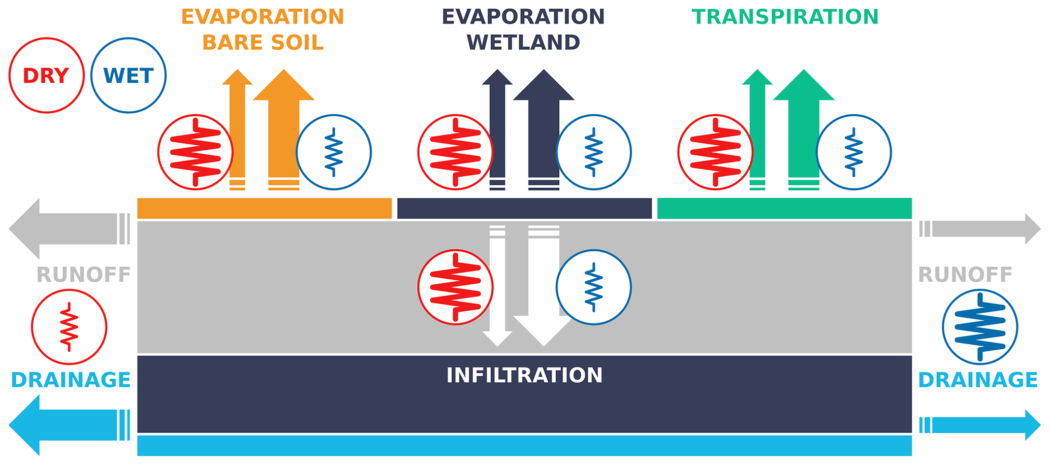
Figure 3JSBACH setups: qualitative comparison between the hydrological fluxes in the DRY and WET JSBACH setups. Shown are bare-soil evaporation (yellow), evaporation from wetlands (dark blue), transpiration (green), infiltration (white), surface runoff (grey) and drainage (light blue), with thick arrows indicating large fluxes and thin arrows small fluxes. The resistances symbols (red in the case of the DRY and blue for the WET setup) indicate whether the parameter settings in a setup facilitate a certain process – indicated by a small resistance symbol – or impede it – indicated by a large resistance symbol. Here, the resistance with respect to bare-soil evaporation and transpiration depends on the parametrization of the maximum water-holding capacity of the uppermost soil layer and of the root zone, respectively. The resistance with respect to evaporation from wetlands is modified via the maximum retention time, which determines the surface water storage and the fractional wetland cover. With respect to infiltration and surface runoff, the resistance depends on the scaling factor FARNO, which allows us to reduce the flux from the surface water storage to the ARNO scheme. The resistance with respect to drainage depends on the assumed mobility of supercooled water as well as on the ice-impedance factor (Fdrain,l).

2.2 Setups
The present investigation is mainly based on two model setups that lead to different degrees of “wetness” in permafrost-affected grid cells – with the meaning of wetness not being limited to the soil water content. The “DRY” setup is characterized by low infiltration rates, poor soil water retention, and large runoff and drainage rates, while the “WET” setup assumes higher infiltration rates combined with high water retention and large evapotranspiration rates (Fig. 3). For the design of the simulations we made use of the optional formulations that were included in the soil hydrology scheme. In the DRY setup, poor soil water retention and high drainage rates are achieved by allowing the supercooled water to move through the ground and by not impeding the lateral drainage in the presence of ice in the subjacent soil layers (Table 1). Low infiltration rates were obtained by setting FARNO to 0.8, and, with respect to evapotranspiration, a high resistance was assumed by including ΔΦorg in and . Finally we use a comparatively low maximum wetland lag (Plag=100 d) which limits the extent of inundated areas and the corresponding infiltration and evaporation rates. For the WET setup, we assumed high infiltration rates, allowing all of the reservoir outflux to be separated into infiltration and surface runoff by the ARNO scheme (FARNO=1). Furthermore, we set a high water retention level in permafrost-affected soils, by assuming that supercooled water is stationary and that the lateral drainage flux is impeded by the ice content of the subjacent soil layers. With respect to evapotranspiration, we assume a low resistance by not accounting for ΔΦorg in and . We also assumed a larger maximum lag for the surface waterbodies (Plag=150 d), resulting in higher evaporative fluxes from inundated areas. Finally, the minimum root depth was increased from 10 to 30 cm, increasing the plant water availability mainly in the mountainous regions in eastern Siberia (not shown).
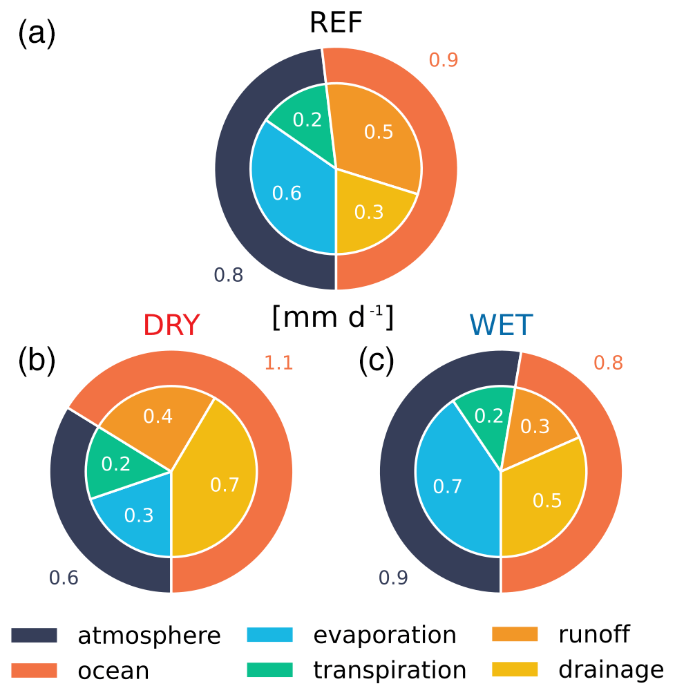
Figure 4Partitioning of hydrological surface fluxes: partitioning of the outgoing moisture fluxes amongst fluxes to the atmosphere and to the ocean (via the river discharge) and further subdivision into evaporation, transpiration, runoff and drainage. Panels show the average over the northern permafrost regions taken from standalone simulations with the atmospheric forcing corresponding to pre-industrial control conditions. The sum of all outgoing fluxes is equal to the precipitation rates, which is the same in all simulations (1.7 mm d−1). Shown is the partitioning for the standard model (REF, a), the DRY setup (b) and the WET setup (c).
As discussed in Sect. 2.1.1–2.1.4, many of the above parameters and optional formulations are a means to represent the uncertainty resulting from the complexity of interactions and processes or from structural shortcomings of the model rather than the uncertainty in the specific parameter values. Thus, they are used for model tuning, even if the specific parameter or formulation itself constitutes a measurable quantity. Furthermore, even if the parameter could at least in theory be better constrained, observation-based information suitable for the resolution of the model may not exist. A good example for this is the maximum wetland lag, which has been determined for specific lakes (Ambrosetti et al., 2003; Brooks et al., 2014), but upscaling the observation-based values to the model scale requires highly uncertain assumptions about the representative bathymetry of wetlands, ponds and lakes and their relative fraction in the overall inundated area. With the number of available tuning options, the design of the setups is – to a certain degree – arbitrary. Here, the differences between the WET and the DRY simulation do not cover the complete uncertainty range included in the parametrizations of JSBACH's soil hydrology scheme. For example, a much drier setup could have been obtained by keeping JSBACH's original formulation of prohibiting infiltration at sub-zero temperatures or maintaining a fixed maximum root-zone soil moisture level – that is, not reducing WMAX,rz by the ice content. Furthermore, we focused on the representation of processes and, besides the minimum root depth, made no diverging assumptions with respect to the soil properties, which are particularly uncertain in regions with large soil organic matter concentrations. Our aim was not to compare the most extreme scenarios but to compare setups whose differences are in the range of “typical” inter-model differences. A measure for the latter was derived from the simulations of the Permafrost Carbon Network Model Intercomparison Project (PCN-MIP; McGuire et al., 2018), which targets the behaviour of state-of-the-art LSMs in permafrost-affected regions (a brief overview of the way the PCN-MIP participants represent key hydrological processes is included in the Supplement (Sect. S1, Table S1), while a detailed analysis can be found in Andresen et al., 2020). Here, our primary focus was the simulated partitioning of moisture fluxes between runoff (including drainage) and evapotranspiration, as this ratio can be expected to be the parameter most relevant for the climate feedback. Thus, we designed the setups in a way that the average differences in evapotranspiration in JSBACH standalone simulations with the WET and the DRY configuration do not (substantially) exceed the standard deviation of the ensemble of PCN-MIP participants (Fig. 4), which is roughly 0.3 mm d−1 (Fig. 2b). A secondary goal was to maintain a similar plant water availability for the same atmospheric conditions so that differences in the vegetation cover in coupled simulations can be fully attributed to the feedback-mediated differences in climate and not to setup-induced soil moisture differences. The agreement with observations was not taken into account in the design of the setups. Nonetheless, we conducted a brief model evaluation – focused on the northern permafrost regions – which is included in the Supplement (Tables S3 and S4 and Figs. S1–S9).
Although the paper focuses on the two setups described above, we performed a third, highly synthetic setup – the W2D setup – which exhibits increasingly dry conditions under future warming. This setup assumes that the characteristics of the soil hydrology are determined by the presence of near-surface permafrost and change when the latter is degraded. All grid cells start with the parametrizations of the WET setup, and the configuration is maintained as long as the model simulates permafrost in the upper 3 m of the soil. However, the parametrizations switch from WET to DRY (with the exception of the soil depths and the maximum wetland retention Plag) whenever the annual maximum thaw depth in the grid cell extends beyond a depth of 3 m. For the high-emission scenario considered in this study, the majority of the grid cells in the northern permafrost regions transition from WET to DRY during the 21st century, with the W2D simulation becoming increasingly different from the WET simulation.
2.3 Simulations
The general setup of the simulations uses a 450 s time step for the atmosphere and land components, while the ocean model is run at a 2700 s time step. The horizontal resolution in the atmosphere and over land is T63 (1.9∘ × 1.9∘) – which corresponds to grid spacing of about 200 km in tropical latitudes – and GR15 (1.5∘ × 1.5∘) in the ocean – which corresponds to 160 km in the tropics. The atmosphere has a vertical resolution of 47 levels reaching up to 0.1 hPa, which is a height of about 80 km, while the ocean model uses 41 vertical layers reaching to a depth of up to 5000 m. The land is resolved by 18 subsurface layers that extend to a depth of about 160 m, 11 of which are used to represent the top 3 m of the soil column. This is very different to the standard vertical setup which represents the soil column by 5 layers reaching to a depth of less than 10 m. Imposing a deeper bottom boundary is important for a realistic representation of the soil thermodynamic regime, with implications for subsurface heat conduction and energy distribution (MacDougall et al., 2008; González-Rouco et al., 2009, 2021), as too shallow LSMs alter the distribution of temperatures in the subsurface (Alexeev et al., 2007; Smerdon and Stieglitz, 2006). As shown by Steinert et al. (2021a) a depth >150 m is required to resemble an infinitely deep soil in climate change simulations of centennial timescales. The improved vertical resolution and bottom boundary condition depth used herein produce changes in the subsurface thermal state that have been shown to interact with the phase changes and other hydrological features. In regions with active layer dynamics, the more realistic conduction of heat from the surface into the soil impacts the depth of the zero annual amplitude of ground temperatures, which has impacts on the simulation of near-surface permafrost extent in the Arctic and subarctic regions (Steinert et al., 2021b). Note that the downward extension of the soil column has no direct impact on the subsurface hydrology as we assume the ground to consist of impermeable bedrock below the soil depth of the standard model configuration.
Both simulations start in the year 1800, with the atmosphere and the ocean being initialized using pre-industrial control simulations with the standard MPI-ESM, which were performed for the CMIP6 DECK experiments. However, the land surface cannot be initialized in the same manner, as the CMIP6 DECK experiments use the standard setup. Thus, they do not include some of the essential variables in permafrost regions – such as the soil ice content – and have a different vertical discretization in the soil. Furthermore, the states that the standard model version simulates in the permafrost regions differ substantially from those simulated with either the WET or the DRY setup. Instead, we used a temperature approximation – based on the surface temperature – to initialize the soil temperature and assumed all soils layers to be close to saturation – that is, at 95 % of the field capacity. Starting from this state, we ran JSBACH in standalone mode for 200 years, with the atmospheric forcing data derived from the MPI-ESM pre-industrial control simulations. During this period, the soil temperatures and soil water and ice content adjust to the prescribed atmospheric conditions, allowing us to use the final states to initialize the coupled simulations.
In the simulations, the water and energy cycles of the MPI-ESM components are fully coupled. However, this is not the case for the biogeochemical cycle. Especially the magnitude of the permafrost carbon feedback is extremely difficult to estimate. Accounting for it in our investigations would have required not only extensive adaptations in JSBACH, but also the performance of a number of ensemble simulations to account for the uncertainty that is included in the formulations of the permafrost carbon cycle (de Vrese et al., 2021; de Vrese and Brovkin, 2021). The latter increases the computational demand of the experiment by an order of magnitude while not necessarily providing any additional insights into the physical land–atmosphere feedbacks in permafrost regions, which are the main focus of this investigation. Instead, we ran the model with prescribed atmospheric greenhouse gas concentrations, which corresponds to the assumption that present-day and future atmospheric CO2 levels are largely determined by human activity and that all variations in the natural carbon fluxes are offset by corresponding adjustments in anthropogenic emissions. The simulations start with an atmospheric CO2 concentration of about 280 ppmv, which increases to about 400 ppmv between the years 1800 and 2014. After 2014, the simulations follow a trajectory of high greenhouse gas (GHG) emissions based on Shared Socioeconomic Pathway 5 and Representative Concentration Pathway 8.5 (SSP5-8.5; van Vuuren et al., 2011). SSP5-8.5 targets a radiative forcing of 8.5 W m−2 in the year 2100 and assumes the atmospheric CO2 concentrations to increase to about 1100 ppmv. We chose to investigate SSP5-8.5, even though it may not be based on the most plausible assumptions (van Vuuren et al., 2011; Riahi et al., 2017; Hausfather and Peters, 2020), but investigating extreme scenarios often helps in highlighting impacts and understanding causal relationships.
Furthermore, we conducted an additional set of simulations in which the atmospheric greenhouse gas concentrations were prescribed in a way as to stabilize the global mean surface temperature at 1.5 ∘C above the pre-industrial CMIP6 ensemble mean temperature. For the DRY setup this required lowering atmospheric CO2 from 450 ppmv in the year 2030 to 400 ppmv in the year 2080. For the WET setup CO2 levels were reduced from 530 to 465 ppmv between the years 2045 and 2095. It should be noted that the differences between these two simulations are a result not exclusively of the differences in model parametrizations but also of the differences in the strength of the CO2 fertilization effect. Without dedicated simulations excluding the effect of rising atmospheric CO2 on vegetation, it is not possible to determine how important the additional 68 ppmv in the WET simulation is for the simulated vegetation covers and the resulting feedbacks on the climate system. However, the WET simulation shows a slightly smaller overall vegetation cover at higher CO2 and the same global mean temperature, indicating that the additional CO2 fertilization is less important than the differences in the spatial distribution of temperatures and precipitation.
2.4 Uncertainty in Arctic and subarctic climate projections
With evapotranspiration rates being partly predetermined – as one of the target variables in the design of our setups (see “Setups” above) – we focus on the uncertainties in simulated surface temperatures and precipitation and how these relate to the evapotranspiration rates. In the northern permafrost regions, the simulations of the CMIP6 ensemble (Table S2) show a high inter-model correlation between precipitation and evapotranspiration – that is, a Spearman's ρ of 0.89 with a p value of for the average over the permafrost-affected grid cells and over the period 2000–2100 (not shown). But, while there appears to be little uncertainty that the two processes are closely connected, it is not clear whether high (low) precipitation rates in a model are caused by high (low) evapotranspiration rates or vice versa or even whether there is little causal relation between the two but a similar dependency on a third factor. Here, our investigation aims to establish or eliminate soil-setup-induced differences in evapotranspiration rates as a potential cause of the variations in high-latitude precipitation between the CMIP6 participants. In contrast, the CMIP6 ensemble exhibits a low correlation between the average surface temperatures and evapotranspiration rates – that is, a ρ of 0.28 with a p value of 0.07. The poor correlation indicates that the surface temperatures are not exclusively determined by the evapotranspiration rates but by a number of factors – one of which may be evapotranspiration. Here, our simulations offer the chance to isolate the potential contribution of permafrost-hydrology-related evapotranspiration differences to the uncertainty in surface temperature in climate change projections.
As a measure of the uncertainty in these projections, we use the inter-model spread of the CMIP6 ensemble, which was derived from 44 simulations provided by 27 modelling groups (an overview table can be found in the Supplement, Table S2). Here, it should be noted that we use the term “inter-model” in a loose sense, as the ensemble does not consist of simulations with 44 different ESMs but includes multiple simulations with the same model being run with a different configuration – e.g. a high vs. a low resolution or with and without interactive vegetation. However, in the case that several simulations were available for the same model configuration but merely differ with respect to the initial conditions or minor parameter settings, we consider only one of the simulations to not underestimate the inter-model spread. To exclude outliers, we do not define the spread as the difference between ensemble minimum and maximum. Instead, we use two frequently applied measures, namely the interquartile range (IQR) – that is, the difference between the 25th and the 75th percentile – and the range contained within 1 ensemble standard deviation of the mean (±σ) – covering about two-thirds of the ensemble if the latter is normally distributed.
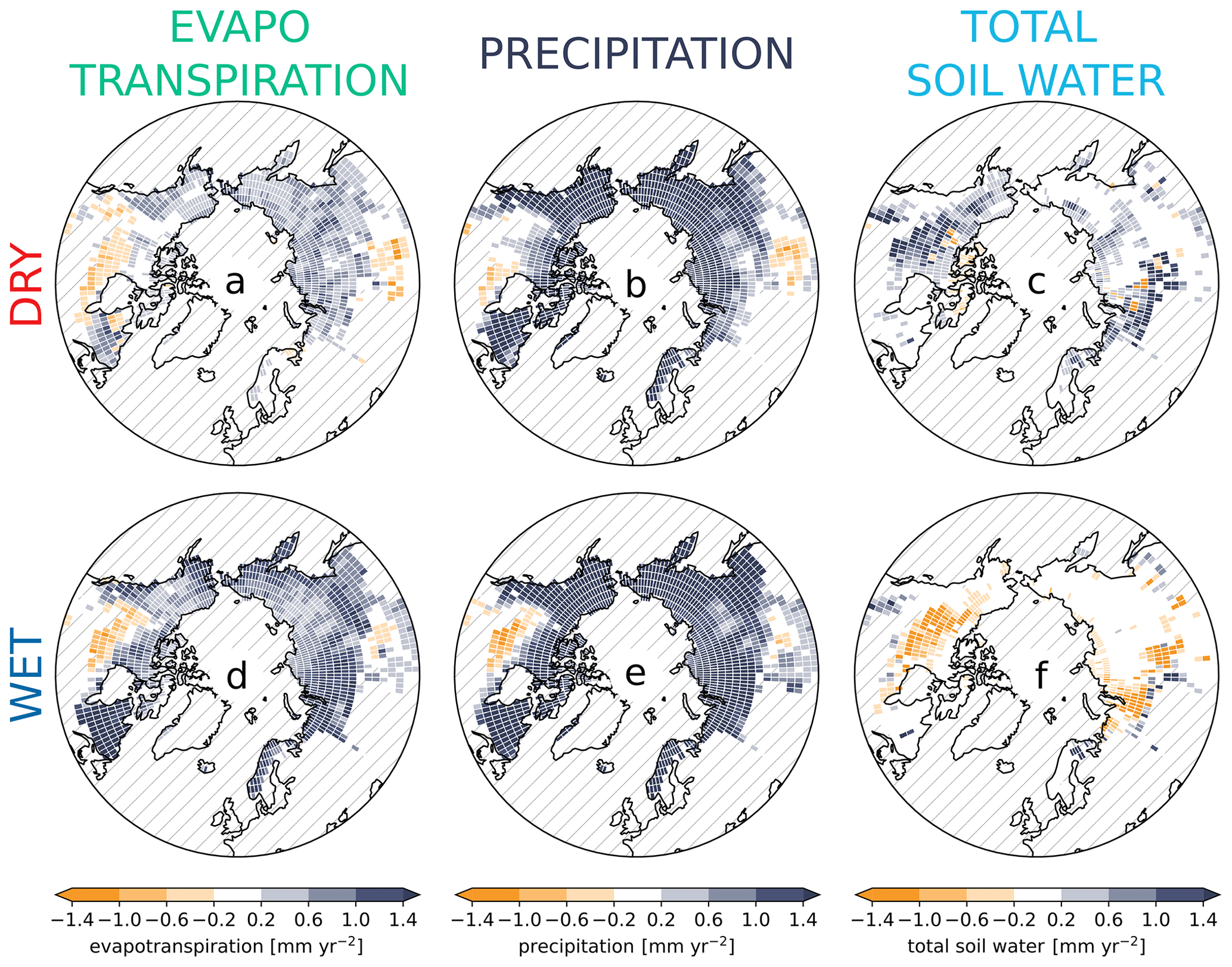
Figure 5Arctic futures: (a) 21st-century evapotranspiration trend in the DRY simulation. (b) Same as (a) but for precipitation. (c) Same as (a) but for the total soil water (liquid soil moisture and ice) content. (d–f) Same as (a)–(c) but for the WET simulation. Trends were estimated applying a simple linear regression to the values covering the period 2000–2099. Non-permafrost and glacier grid cells are hatched.
3.1 Land–atmosphere interactions
One of the questions that motivated this investigation is whether the Arctic and subarctic zone will become wetter or drier in response to future warming or rather if present-day ESMs can be used to predict this with some degree of confidence, given the uncertainties in the hydrology parametrizations of the land surface components. Both the WET and the DRY simulation predominantly show an increase in evapotranspiration and precipitation, even though the signal is not uniform across the northern permafrost areas (Fig. 5a, b, d, e). Especially in North America there are extensive regions in which the evapotranspiration rates decline during the 21st century. These regions enclose most of the areas that also exhibit a negative trend in precipitation, indicating that the latter is the result of reduced moisture recycling. Nonetheless, the general trend is an increase in the intensity of the hydrological cycle with the signal being more pronounced in WET than in DRY. In contrast, the two simulations show opposing trends in the total soil water content – that is, liquid water and ice (Fig. 5c, f). In WET, the soils in most grid cells lose water, with the trend being partly driven by a strong increase in the drainage rates (not shown). In this setup, lateral drainage is strongly inhibited in the presence of ice and the marked increase in these fluxes is the result of the warming-induced decrease in the soil ice concentration. In the DRY setup, the inhibition of the lateral subsurface flow in the presence of ice is less severe; hence, the increase in drainage due to permafrost degradation is less pronounced. As a result, the soils in the DRY simulation almost exclusively exhibit an increase in the water content, with the increase in precipitation (− evapotranspiration) being the dominant signal. It should be noted that JSBACH, as with most land surface models, does not include a representation of excess ice. Excess ice is the water that the soil can only hold when frozen but that exceeds the pore volume of the unfrozen ground. Thus, the thawing process effectively reduces the amount of water that the soils can hold, and it is plausible that the increase in the water content found in the DRY setup – and also found in other models (Andresen et al., 2020) – is only possible because the model neglects the feature of a higher soil water-holding capacity in the frozen state.
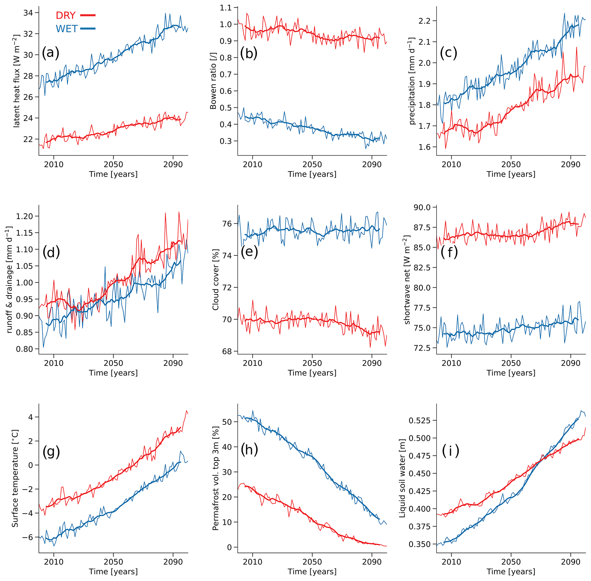
Figure 6Effects of soil hydrological conditions on near-surface climate: (a) latent heat flux in the northern permafrost regions in WET (blue) and DRY (red) MPI-ESM simulations for SSP5-8.5. Thin lines show the annual mean, averaged over the northern permafrost regions (note that grid cells covered by glaciers were excluded), while thick lines give the 10-year running mean. (b–i) Same as (a) but showing (b) the Bowen ratio, (c) precipitation, (d) surface runoff and drainage, (e) accumulated cloud cover, (f) solar radiation absorbed at the surface, (g) surface temperatures, (h) near-surface (top 3 m of the soil) permafrost volume, and (i) liquid soil water content.
Thus, when considering the total soil water content to be a key indicator, the uncertainty in the representation of the permafrost hydrology makes it impossible to provide an unambiguous answer to the question whether the Arctic and subarctic region will become wetter or drier in the future. Furthermore, the agreement on the direction of the trends in evapotranspiration and precipitation does not mean that the different soil hydrology setups entail similar conditions at and above the surface. On the contrary, the land–atmosphere interactions diverge substantially between WET and DRY, which has a distinct impact on the near-surface climate. In WET, the evapotranspiration rates are between 0.2 and 0.3 mm d−1 larger than in DRY, which translates into a difference in latent heat flux of about 5 W m−2 at the beginning and about 9 W m−2 at the end of the 21st century (Fig. 6a). The additional evaporative cooling in WET constitutes 6 % to 10 % of the shortwave radiation that is absorbed by the surface and profoundly changes the partitioning of the surface energy budget. With the Bowen ratio decreasing to 0.3, the permafrost-affected areas are increasingly energy limited in WET, while in DRY, a Bowen ratio of almost 1 indicates that at least parts of the region experience some degree of water limitation (Fig. 6b).
With less sensible heat and more latent heat being transferred into the atmosphere, the boundary layer is initially cooler and moister in WET than in DRY (not shown). This leads to higher relative humidity and, consequently, to precipitation rates that are roughly 0.2 mm d−1 larger in WET (Fig. 6c). The higher precipitation rates in turn increase the soil water availability, establishing a positive feedback in which the more intense moisture recycling is the main factor sustaining the higher evapotranspiration rates. More specifically, about 80 % of the additional evapotranspiration in WET is compensated for by higher precipitation rates, while merely 20 % is balanced by differences in runoff (Fig. 6d). Furthermore, the differences in relative humidity result in differences in the cloud cover, which constitute another important feedback on the surface energy balance (Fig. 6e). The increased cloudiness in WET occurs mainly during the snow-free period – spring to early autumn in the southern permafrost regions, with the length of the period decreasing in a northward direction – when the surface reflectivity is determined by a comparatively dark vegetation cover and similarly dark bare-soil areas. Thus, the more extensive cloud cover notably raises the planetary albedo (relative to DRY), reducing the surface incoming solar radiation by between 10 W m−2 at the beginning and 13 W m−2 at the end of the 21st century. When additionally taking into consideration the differences in the surface reflectivity – resulting from differences in the simulated snow and vegetation covers – the differences in absorbed shortwave radiation amount to roughly 12 W m−2 (Fig. 6f). The reduction in the available energy cools the surface further, which leads to less sensible heat being transferred into the boundary layer, contributing to the higher relative humidity in the atmosphere. Here, it should be noted that the differences in evaporative cooling and those in the planetary albedo affect the available energy very differently because the former mainly redistribute while the latter provide a net change to the energy content of the system. However, even when focusing exclusively on the surface latent heat flux and the incoming shortwave radiation, the cloud effect (10–13 W m−2) has a larger impact on the surface energy balance than the evaporative cooling that initially caused it (5–9 W m−2).
The energy balance determines the temperatures at and below the surface, which in turn are highly relevant for the question whether the high latitudes will become wetter or drier in the future. It can be argued that a more suitable measure for the wetness of the permafrost areas is the liquid – rather than the total – water content of the soils, with the former controlling the majority of the physical and biophysical land processes. Here, the trend in liquid soil moisture depends not only on the development of the total water content, but also on the temperature evolution, as these determine the ratio of liquid and frozen water in the soil (Fig. 6g). In both simulations, the 21st-century warming results in a substantial decline in the extent and thickness of the near-surface permafrost (Fig. 6h; note that the near-surface permafrost volume corresponds to an initial permafrost area of about 22×106 km2 in WET and about 16×106 km2 in DRY; at the end of the 21st century the values are 11×106 and 4×10⁶ km2, respectively), leading to a marked decrease in the soil ice content and a corresponding increase in liquid water (Fig. 6i). Thus, when basing the question of future wetness on the liquid soil water content, our simulations provide a clear answer: the trends in evapotranspiration, precipitation and soil moisture all suggest that, on average, the Arctic and subarctic region will become wetter in the future. This general trend appears to be a robust feature, the direction of which is independent of the representation of the permafrost hydrology in the model. However, the magnitude of the (liquid) soil moisture trend is very sensitive to the parametrization of the model, mainly to the resulting differences in the simulated surface temperatures. Here, the WET simulation is consistently colder, which results in a higher near-surface permafrost volume at the beginning of the 21st century and a lower liquid soil moisture content. With the higher initial permafrost volume, the 21st-century warming has a more pronounced impact on the thaw rates, and the resulting trend in the liquid soil moisture is much larger in WET than in DRY, despite WET exhibiting a negative trend in the total soil moisture (Figs. 5c and f and 6i).

Figure 7Comparison to CMIP6 ensemble – annual means: (a) simulated differences in evapotranspiration in permafrost regions and the respective CMIP6 ensemble spread. The black line shows the differences between WET and the DRY (), the green area gives the interquartile range (IQRevap) – that is, the difference between the 75th and the 25th percentile – of the CMIP6 ensemble, and the grey area provides 2× the ensemble standard deviation (±σevap). (b, c) Same as (a) but for (b) precipitation (, IQRpr, ±σpr) and (c) surface temperatures in permafrost grid cells (, IQRts, ±σts). Shown are annual means.
3.2 Differences in climate compared to the CMIP6 spread
Another question motivating our study was to which extent differences in the parametrizations of the soil hydrology could help explain the large inter-model spread that the present generation of ESMs exhibits in the Arctic and the subarctic zone. In the northern permafrost regions, the absolute value of the differences in evapotranspiration between DRY and WET () captures the range of typical inter-model differences comparatively well, and at the beginning of the 21st century they match the respective interquartile range of the CMIP6 ensemble (IQRevap) almost perfectly (Fig. 7a). Subsequently, increases considerably, exceeding IQRevap by 2030, but remains well within the range of 2 (CMIP6) ensemble standard deviations (±σevap). It should be noted that this good agreement was to be expected as the setups were designed to produce differences that do not exceed the range of typical evapotranspiration differences between commonly used LSMs (although these typical differences were not determined based on fully coupled CMIP6 simulations but on the ensemble of standalone simulations that were performed for the PCN-MIP). Thus, the more interesting question is how sensitive the simulated climate is to these differences in evapotranspiration, more specifically whether the latter lead to differences in other key variables that are similarly consistent with the respective CMIP6 spreads.
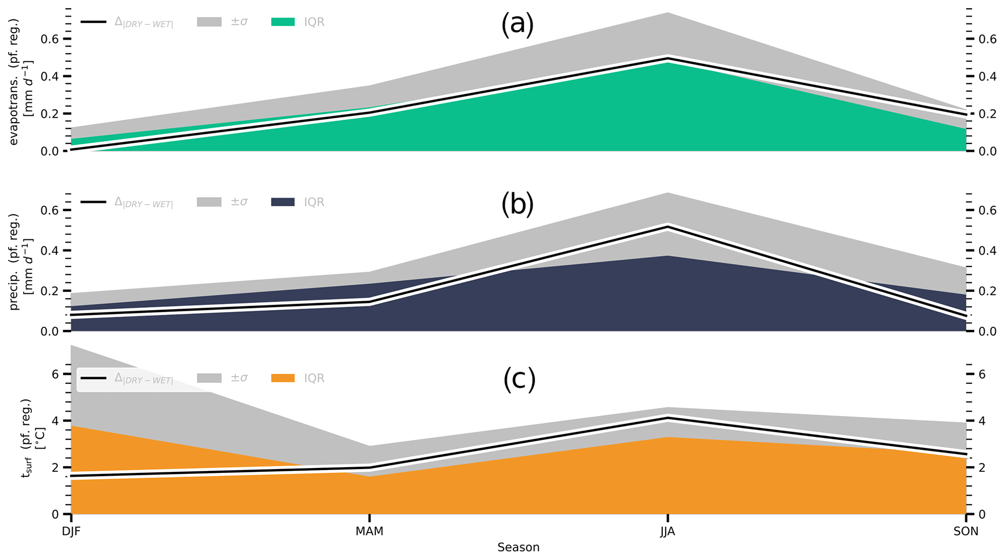
Figure 8Comparison to CMIP6 ensemble – seasonality: (a) simulated differences in evapotranspiration in permafrost regions and the respective CMIP6 ensemble spread. The black line shows the differences between WET and the DRY (), the green area gives the interquartile range (IQRevap) – that is, the difference between the 75th and the 25th percentile – of the CMIP6 ensemble, and the grey area provides 2× the ensemble standard deviation (±σevap). (b, c) Same as (a) but for (b) precipitation (, IQRpr, ±σpr) and (c) surface temperatures in permafrost grid cells (, IQRts, ±σts). Shown is the seasonality averaged over the 21st century.
In the case of precipitation, the differences in the soil hydrology parametrizations appear to offer a large explanatory potential (Fig. 7b). On average amounts to about 0.16 mm d−1, IQRpr to about 0.19 mm d−1 and ±σpr to 0.32 mm d−1. Thus, even if considering ±σpr to be the more appropriate measure, about half of the inter-model spread of the CMIP6 ensemble may be explainable by diverging evapotranspiration rates resulting from differences in the parametrizations of the permafrost hydrology. Here, exhibits a marked peak in the summer months, when the causative differences in evapotranspiration are largest (Fig. 8a, b). A similar behaviour can be seen for the ensemble spread, even though the (relative) seasonal variations are less pronounced, especially in the case of IQRpr. With regards to the surface temperatures, matches the overall magnitude of the CMIP6 ensemble spread similarly well (Fig. 7c), with being equal to IQRts (2.6 ∘C) and representing about two-thirds of ±σts (3.7 ∘C). However, as with the differences in precipitation, peaks – at 4.2 ∘C – when the differences in evapotranspiration are largest (Fig. 8c), which is not the case for IQRts and ±σts. While the latter exhibit a notable increase in summer, their annual maximum occurs during winter – with 3.8 and 7.2 ∘C, respectively – when is the lowest. As described above (Sect. 3.1), the differences between WET and DRY mainly originate from a divergence of the cloud cover and the resulting differences in the planetary albedo. But as there are only minor differences in cloudiness – and very little solar radiation – during the snow cover season, this feedback is not present during the winter months. More importantly, the cloud radiative effect differs between the snow-covered and the snow-free period. The albedo of clouds is similar to those of snow- and ice-covered surfaces, and an increase in cloudiness does not lower the planetary albedo in winter. Instead, (low) clouds are more likely to increase the surface temperatures as they raise the surface net radiation by reflecting the longwave radiation emitted by the surface (Vihma et al., 2016). Thus, it is mainly the differences in soil heat content – resulting from differences in the energy uptake during the snow-free period – and differences in latitudinal heat transport (not shown) that sustain during winter, while it is most likely differences in the parametrization of the snow and ice albedo that determine the large ensemble spread (Menard et al., 2021). Consequently, the explanatory power of the differences in the soil hydrology parametrizations appears to be limited to the snow-free period.
Furthermore, shows a good agreement with the inter-model spread especially during the first half of the century, ranging between IQRts and ±σts. During the second half of the century, both IQRts and ±σts increase by more than 1 ∘C, while shows no significant increase. Thus, matches the magnitude of the CMIP6 spread well but appears to lack an important dynamical component. It may appear counterintuitive that the temperature differences between WET and DRY remain fairly constant during the 21st century despite the difference in evapotranspiration and evaporative cooling increasing over time. The reason for this is that evapotranspiration initially lowers the temperatures at the surface, but it eventually increases the air column temperature by the heat release during condensation. Thus, the evaporative cooling redistributes energy between latent and sensible heat and between surface and atmosphere but does not change the energy content of the coupled land–atmosphere system. The combination of lower surface temperatures and higher atmospheric temperatures, in turn, increases the downward fluxes of sensible heat and longwave radiation or decreases the upward fluxes, which largely balances the effect of the evaporative cooling at the surface. Over longer periods, local surface temperatures only change significantly if the evaporated or transpired water is advected out of the region and the net effect can be approximated by the latent heat included in the precipitation − evapotranspiration difference (P−E). Here, WET and DRY exhibit similar trends – as indicated by the trends in surface runoff and drainage (Fig. 6d; note that over longer periods P−E ∼ runoff and drainage) – and the difference in P−E remains constant over time. Furthermore, the divergence of the evapotranspiration rates results in increasingly large differences in the cloud cover, affecting the planetary albedo. In contrast to the evaporative cooling, the albedo differences change the amount of energy reflected back to space, hence the total energy content of the system. However, the albedo effects resulting from the divergence in the cloud cover are compensated for by decreasing differences in the surface reflectivity, mainly resulting from a convergence of the simulated vegetation covers. As a result, the differences in absorbed shortwave radiation do not change over time (Fig. 6f) and, with no significant trends in the differences in either P−E or the planetary albedo, the temperature differences between WET and DRY remain almost constant during the 21st century.
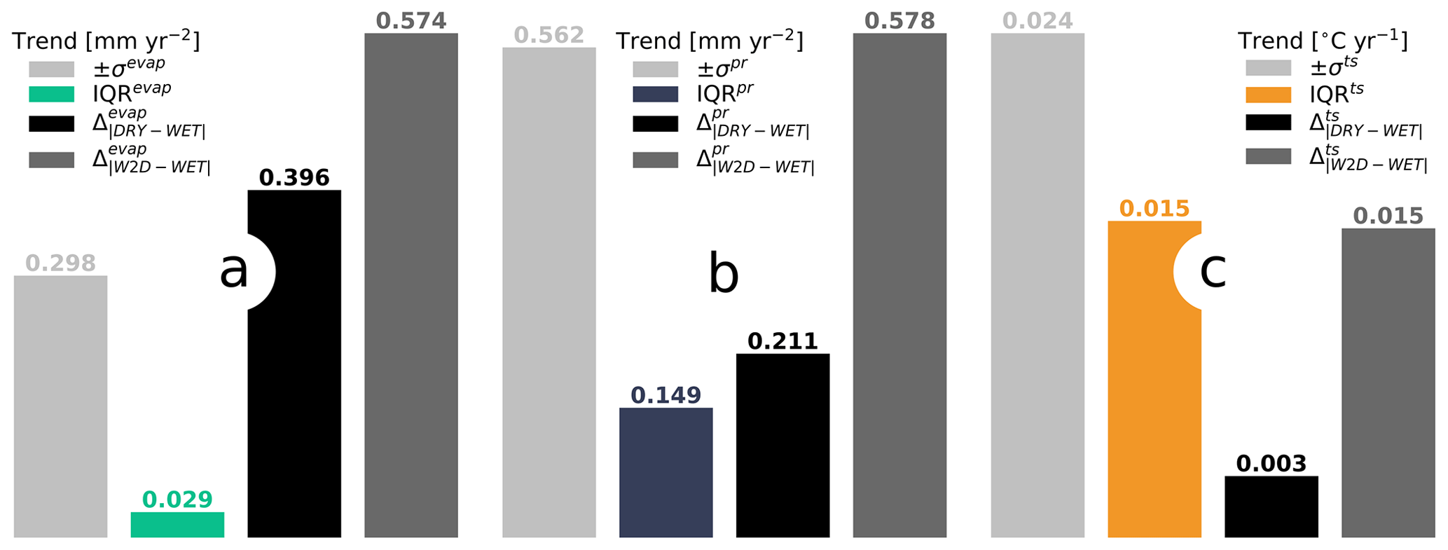
Figure 9Comparison to CMIP6 ensemble – 21st-century trends: (a) trends in evapotranspiration during the 21st century with 2× the CMIP6 ensemble standard deviation, the interquartile range of the CMIP6 ensemble, differences between WET and DRY, and differences between W2D and WET – averaged over the northern permafrost regions. (b, c) Same as (a) but for (b) precipitation and (c) surface temperatures. Trends were estimated applying a simple linear regression to the values covering the period 2000–2099.
This raises the question whether the uncertainty in the permafrost hydrology is insufficient to explain the increase in the inter-model spread, especially during the second half of the century, or whether the issue of constant temperature differences is specific to our setups. Per design, the simulations with the WET and the DRY setups become more similar over time as many of the distinctions depend on the soil ice content, which decreases throughout the simulation. To test how far the lack of trends is related to this design feature, we compared the WET simulation to a simulation with the W2D setup. In the W2D simulation, the parametrizations switch from WET to DRY when the near-surface permafrost disappears in a given grid cell, with the W2D simulation becoming increasingly different from the WET simulation. With respect to precipitation and surface temperature, the differences between W2D and WET exhibit trends that are substantially larger than those in the differences between DRY and WET (Fig. 9b, c). The trend in is also larger than the trend in and IQRpr, closely matching the trend in ±σpr, while the trend in the temperature differences, , is very similar to the trend in IQRts. This indicates that differences in soil hydrology parametrizations may, in principle, contribute to the trend of the inter-model spread, given that the parametrizations do not become more similar with the advancing permafrost degradation. Here, however, the trends in and stem from a much larger causative trend in the evapotranspiration differences, (Fig. 9a). The latter is almost twice as large as the trend in ±σevap and almost 20 times larger than the trend in IQRevap, strongly suggesting that the trends in the temperature spread of the CMPI6 ensemble are not caused exclusively by the divergence of evapotranspiration rates (Hahn et al., 2021).
3.3 Relevance for global climate and the state of tipping elements
While the above results show that the differences in the parametrization of the permafrost hydrology may not fully explain the spread of the CMIP6 ensemble – especially the latter's seasonality and 21st-century trend – the differences in simulated climate of the continental permafrost areas are substantial. This raises the question whether the respective effects are confined to this region or whether they are relevant for the climate on larger scales. Non-glaciated, permafrost-affected areas only cover about a third of the Arctic and subarctic zone. Yet averaged over the planet's surface north of 50∘ N, the temperature differences between WET and DRY () amount to about 2.0 ∘C (Fig. 10). This is notably less than but still more than twice as much as would have been the case if the temperature effects were limited to the land areas affected by permafrost, indicating that the permafrost hydrology is indeed relevant for the entire region, including glaciers and the ocean.
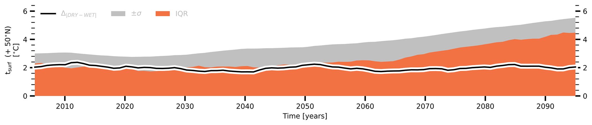
Figure 10Comparison to CMIP6 ensemble – surface temperature north of 50∘ N: (a) simulated differences in evapotranspiration in regions (land and ocean) north of 50∘ N and the respective CMIP6 ensemble spread. The black line shows the differences between WET and the DRY (), the red area gives the interquartile range (IQR) – that is, the difference between the 75th and the 25th percentile – of the CMIP6 ensemble, and the grey area provides 2× the ensemble standard deviation ().
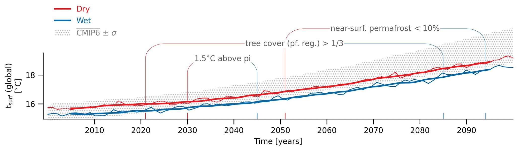
Figure 11Effect on global climate: simulated global mean surface temperatures for the DRY (red) and the WET (blue) setups and range of the CMIP6 ensemble mean ± 1 standard deviation for the SSP5-8.5 scenario. Shown are the points in time at which the tree cover in permafrost-affected regions exceeds one-third of the surface area, the simulated global mean surface temperature reaches 1.5 ∘C above pre-industrial levels (with the latter being based on the CMIP6 ensemble mean temperature) and the near-surface permafrost volume decreases below 10 %.
Arctic and subarctic temperatures constitute the main drivers of a number of important processes, some of which have implications for the global climate. For example, the magnitude of the permafrost carbon feedback is largely determined by the speed with which the vast pools of soil organic matter in the Arctic and subarctic zone will become exposed to conditions that are required for microbial decomposition and hence by the rate of permafrost thaw. As shown above, the simulated degradation of the terrestrial permafrost is very different in WET and DRY and the point in time when the near-surface permafrost (almost) disappears from the northern high latitudes differs by about 50 years (Fig. 11). The terrestrial net carbon flux in the Arctic and subarctic region also depends on the trend in Arctic greening, as the expanding vegetation takes up increasingly large amounts of atmospheric CO2 (Qian et al., 2010; Keenan and Riley, 2018; Pearson et al., 2013; McGuire et al., 2018; Zhang et al., 2018). Here, the surface temperatures determine the length of the growing season, with leading to substantial differences between the simulated vegetation dynamics in WET and DRY. For example, the moment after which the tree cover exceeds a third of the land surface in the permafrost-affected regions differs by more than 60 years between the two simulations. Both processes, permafrost degradation and Arctic greening, are highly relevant for the atmospheric greenhouse gas concentration but are not the only ways for permafrost hydrology to affect the global climate.
Temperature differences in the Arctic and subarctic zone modulate the latitudinal temperature gradient, causing a change in the meridional heat transport which leads to a southward propagation of the temperature signal. In fact, the differences in the permafrost hydrology impact the total energy content of the Earth system to such an extent that surface temperatures across the entire Northern Hemisphere are significantly affected. Thus, the global mean temperature in WET and DRY differs by about 0.5 and 0.6 ∘C at the beginning and the end of the 21st century, respectively (Fig. 11), despite the non-glaciated, permafrost-affected areas in the Arctic and subarctic region covering merely 5 % of Earth's surface. Here, 0.5–0.6 ∘C constitutes substantial differences, not only in comparison to the CMIP6 ensemble spread, but also relative to the temperature increase during the 21st century. In the case of the high-emission scenario SSP5-8.5, the point in time when the simulations reach the same global mean temperature differs by about 15 years (Fig. 11). And because the albedo differences affect primarily the Arctic and subarctic region, this global mean temperature is reached with a substantially different latitudinal distribution – with the DRY simulation exhibiting predominantly higher temperatures in the northern high and middle latitudes, while the temperatures are significantly lower throughout the tropics (Fig. 12a).
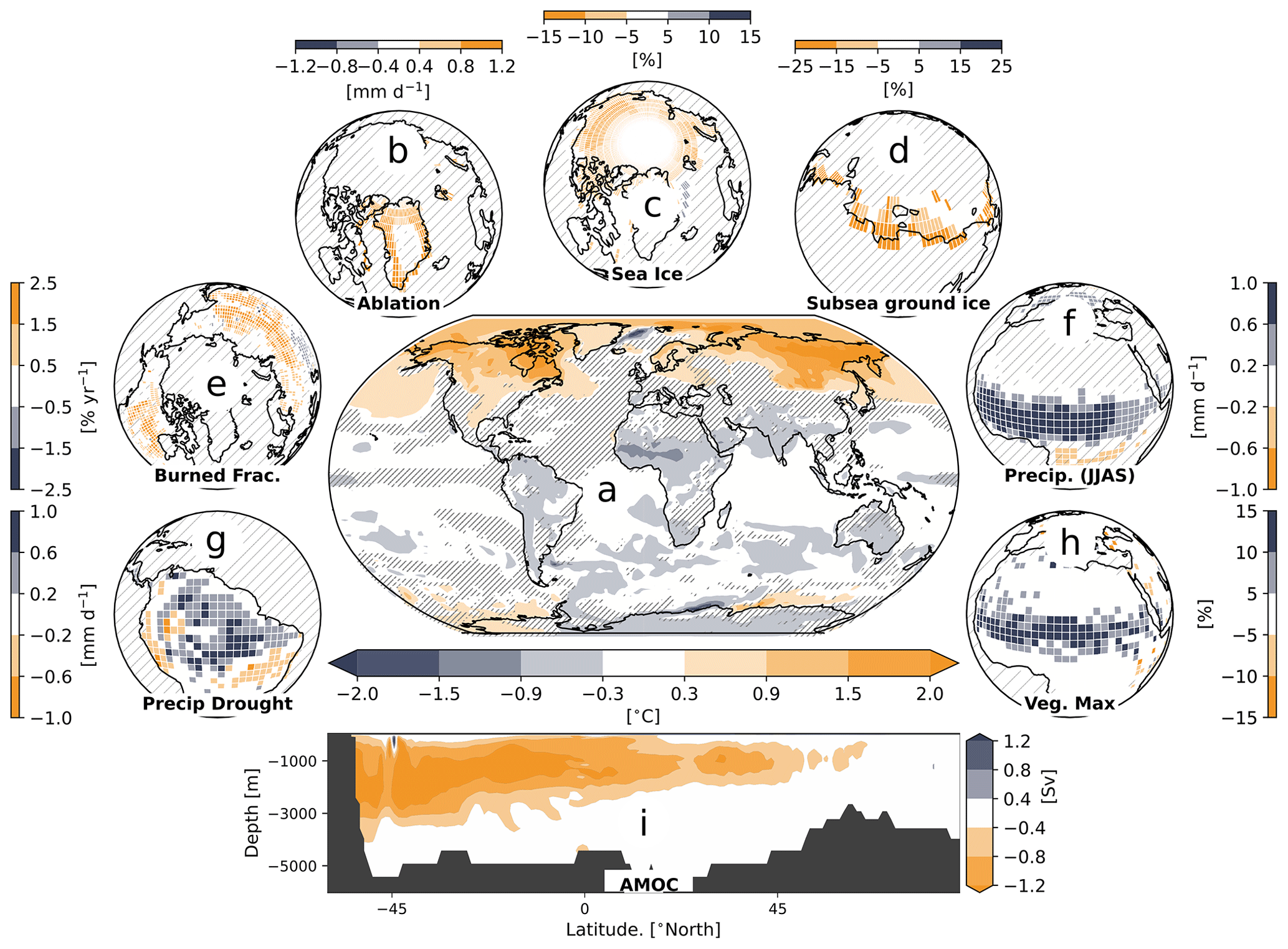
Figure 12State of tipping elements and other core climate elements at 1.5 ∘C above the pre-industrial mean: (a) differences in the annual mean surface temperatures between the DRY and the WET setup for a global mean surface temperature of 1.5 ∘C above the pre-industrial CMIP6 ensemble mean. Shown is the difference between simulations in which the atmospheric greenhouse gas concentrations were modified to stabilize the climate for a 50-year period. (b–d) Same as (a) but for (b) glacier ablation rates, (c) annual average Arctic sea-ice concentration and (d) relative difference in subsea permafrost volume within the top 10 m of the subsurface. Shown is the Laptev Sea and the East Siberian Sea. Panel (d) is not based on simulations with the MPI-ESM but on simulations with an adapted JSBACH model that represents the permafrost dynamics on the Arctic shelves using the bottom temperatures from DRY and WET. A detailed description of this model version is given in Wilkenskjeld et al. (2022). (e–i) Same as (a) but showing the (e) (annually) burned area in boreal regions, (f) precipitation during the West African monsoon, (g) minimum 3-year mean precipitation in the Amazon Basin, (h) vegetation cover in the region of the West African monsoon and (i) strength of the Atlantic Meridional Overturning Circulation. Shown is the 50-year mean. In panels (a)–(f) and (h), areas where differences are not significant (p value >0.05) are hatched, while panel (g) shows the minimum 3-year mean precipitation over land during the 50-year period without a test of significance. Dark grey areas in panel (i) show the bathymetry of the Atlantic Ocean.
The sustainability of a given climate trajectory depends on the associated risks for natural and human systems (IPCC, 2018), some of which stem from regional tipping elements (Lenton et al., 2019), such as the West African monsoon, reaching a critical threshold. How close these elements are to a tipping point at a given global mean temperature depends on the latitudinal temperature gradient which determines the local temperature change. For a climate stabilization at a desirable level – e.g. 1.5 ∘C above the pre-industrial mean – the state of many tipping elements in the northern cryosphere is distinctly different between DRY and WET. The near-surface permafrost volume in the northern high latitudes is 15 %–30 % lower in DRY than in WET, and the ablation rates of the Greenland ice sheet differ by up to 1 mm d−1. In addition, the annual mean Arctic sea-ice concentration is reduced by up to 15 % (Fig. 12b, c) in the DRY simulations. The difference in the simulated ice coverage is particularly prominent during the summer months with the DRY simulation featuring an almost ice-free Arctic Ocean, while around 2×10⁶ km2 remains ice-covered in the WET simulation (not shown). In the SSP5-8.5 simulations, the differences during summer are even more pronounced, with the DRY simulations reaching an ice-free state several decades before the WET simulations. These findings, again, shed interesting light on the regional differences in the temperature response to the two scenarios. For a given model, as well as for the observational record, a clear, linear relationship between global mean temperature and Arctic sea-ice coverage has long been identified across all months (Gregory et al., 2002; Mahlstein and Knutti, 2012; Niederdrenk and Notz, 2018). However, our investigation now shows for the first time that for a given model the same global mean temperature, in our case a warming of +1.5 ∘C, can result in differences in the simulated sea-ice coverage owing to differences in the regional amplification of the global temperature signal. Our simulations also show that these differences are not necessarily equally pronounced across all months, as the sea-ice concentrations in March in the SSP5-8.5 simulations are barely distinguishable between the WET and the DRY simulations, while they are clearly different in September.
The sea-ice cover has a strong effect on the benthic temperatures, which, in turn, determine the state of the roughly 3.5×10⁶ km2 of permafrost soils that has been submerged since the Last Glacial Maximum and forms a large part of the Arctic Shelf (Sayedi et al., 2020; Steinbach et al., 2021). The permafrost-affected sediments hold about 500 Gt of organic carbon and methane gas, with continuous thawing from the surface increasing the vulnerability of the carbon pools (Schuur et al., 2015). Here, the subsea permafrost extent near the sea bottom is strongly affected by the temperature differences between DRY and WET, in particular in the Laptev Sea and the East Siberian Sea where the frozen fraction in the top 10 m of the subsurface differs by up to 50 % (Fig. 12d; note that the subsea permafrost was diagnosed with a different model version, which is described in Wilkenskjeld et al., 2022).
In the boreal zone, the differences in the simulated temperatures and vegetation covers have a strong impact on the frequency and extent of wildfires. In DRY, the burned grid-cell fraction is up to 2 % yr−1 larger, reaching up to 10 times the area burned in WET (Fig. 12e). Furthermore, the strength of the Atlantic Meridional Overturning Circulation (AMOC) is partly determined by the rate with which the surface currents cool in the North Atlantic. The lower latitudinal temperature gradient in DRY reduces this part of the thermohaline circulation, weakening the AMOC by up to 1.5 Sv (106 m3 s−1) in both the North and the South Atlantic Ocean (Fig. 12i). However, not all tipping elements are closer to the critical threshold due to the smaller temperature gradient in DRY. Most prominently, the position and latitudinal oscillation of the Intertropical Convergence Zone is shifted, which results in a higher intensity of the West African monsoon in DRY. Precipitation rates during the period June–September increase by up to 1 mm d−1 relative to WET, which constitutes up to 70 % of the precipitation in the Sahel zone (Fig. 12f). This difference in the monsoon precipitation increases the plant-available water, and the simulated vegetation cover is up to 15 % larger in DRY than in WET (Fig. 12h). In the Amazon Basin, the precipitation rates during multi-annual periods of low precipitation (here 3 years) are up to 1 mm d−1 larger in DRY (Fig. 12g). This corresponds to a relative difference of up to 40 % of the drought precipitation and may have implications for a potential dieback of the Amazon rainforest.
The above examples are by no means a complete list of the remote effects resulting from the differences in the permafrost hydrology. However, they clearly show how important the respective parametrizations are for the global climate, even though the northern permafrost regions make up only a small part of the land surface.
As described in the Methods section, our JSBACH setups were designed to reproduce typical inter-model differences and they manage to quantitatively capture the spread in the ensemble of PCN-MIP simulations reasonably well. However, it is exceedingly difficult to assess if our setups also adequately reflect the variability in the parametrizations employed by current-generation land surface models, as it is highly uncertain what causes the diverging hydrological fluxes and states in the PCN-MIP participants. Andresen et al. (2020) suggested the representations of evapotranspiration, soil organic matter, the water table – which in some models is used to estimate infiltration rates – and the vertical movement of water through the ground are important sources of uncertainty in the models' soil hydrology schemes. However, even their detailed analysis did not resolve how specific implementations affect the hydrological processes or quantify the contribution of individual factors to the overall uncertainty.
One reason why it is so difficult to identify the key drivers of uncertainty is that it is often not one specific parametrization but the interactions between processes that determine the behaviour of a given model. For example, the impact of supercooling on the state of the land surface and the hydrological fluxes may depend strongly on the assumptions with respect to the mobility of the supercooled water and whether or not the water is assumed to be available to plants. This is particularly problematic as differences in the simulated soil hydrology may also originate from differences in the treatment of the soil thermal dynamics – as these determine the state of water in the soil – as well as from differences in the general model setup, e.g. vertical resolution and depth of the soil column and the representation of vegetation. Thus, our results can merely estimate the bulk effect of the uncertainty included in the range of established soil hydrology representations without trying to connect them to specific formulations employed by present-day land surface models.
It is very difficult to judge whether one of the setups actually simulates a present-day climate that is closer to observations, which could be taken as an indicator for a better representation of the processes and may even suggest which future climate trajectory is more likely for a high-emission scenario. Here, an evaluation yields ambiguous results with none of the setups showing a better agreement with the observations for all the variables considered in the comparison (see Figs. S1–S9). For example, the WET setup simulates surface temperatures that are much closer to observations, while the DRY setup exhibits a lower bias with respect to the permafrost temperatures and precipitation rates. This ambiguity of the results does not necessarily mean that both setups are similarly ill-suited to representing the northern permafrost regions, as such a comparison can only evaluate the performance of the ESM as a whole but may be less revealing for individual components of the model. Thus, even if one of the setups provides a more realistic representation of the processes, it may increase the bias in a given variable simply by removing a compensating error. However, another possible explanation is that neither the WET nor the DRY setup is capable of representing the broad spectrum of soil conditions and processes that determine the land–atmosphere interactions across the entire region. Similarly to W2D, a suitable setup may require different parametrizations in specific grid cells, which may also vary depending on the state of the soil. This, however, is very difficult to achieve in the often highly heterogeneous northern permafrost regions where wet and dry conditions may coexist in close proximity and different parts of a grid cell are better represented by either of the setups.
Here, one potential strategy is to increase the horizontal resolution of the model to a point at which the spatial heterogeneity is resolved. But, while it is feasible to run the LSM in a standalone mode over a limited domain, using a resolution of a few metres, it will likely remain impossible for quite some time to run a fully coupled ESM over longer periods with a resolution approaching the kilometre scale. Another way to increase the “resolution” of the model is to introduce additional layers of tiling, with the added tiles representing different factors that determine the hydrological conditions and the land–atmosphere interactions. Such tiling would need to account not only for the subgrid-scale variations in the soil properties but also for the numerous processes that redistribute water horizontally within the grid cell. With respect to the former, suitable data already exist for a large number of soil properties, but for other important parameters – such as the distribution of ice wedges – high-resolution data are not available on the pan-Arctic scale. For the treatment of the lateral movement of water, the current generation of LSMs requires a number of new sub-modules that account not only for the moisture variability on the sub-metre scale, e.g. in the polygonal tundra, but also for the lateral fluxes from high- to low-lying areas along gradient slopes that act on the scales of tens to thousands of metres (Cresto Aleina et al., 2013; Aas et al., 2019; Nitzbon et al., 2021; Smith et al., 2022). Given that this will require at least one additional layer of tiles and that the hydrological conditions may vary over short periods of time, which results in comparatively fast changes in the tile fractions, this approach requires a flexibility in the model structure which few of the present-day LSMs possess.
Finally, please note that the present investigation relies exclusively on simulations with the MPI-ESM. However, to confirm that our findings do not merely describe a specific feature of this particular model, but also provide more general insights, we conducted an additional set of simulations with the new ICON Earth System Model (ICON-ESM; Jungclaus et al., 2022). A brief overview of the respective results is included in the Supplement (Sect. S4).
The primary data are available via the German Climate Computing Center long-term archive for documentation data (https://www.wdc-climate.de/ui/entry?acronym=DKRZ_LTA_1219_ds00001; de Vrese et al., 2022). The model, scripts used in the analysis and other supplementary information that may be useful in reproducing the authors' work are archived by the Max Planck Institute for Meteorology and can be obtained by contacting publications@mpimet.mpg.de.
The supplement related to this article is available online at: https://doi.org/10.5194/tc-17-2095-2023-supplement.
PdV, JFGR, DN, TS, NJS, SW and VB designed the experiment. PdV, TS and SW performed simulations. PdV, GG, DN and VB conducted analysis and validation of simulations. All authors contributed to and reviewed the manuscript.
The contact author has declared that none of the authors has any competing interests.
Publisher's note: Copernicus Publications remains neutral with regard to jurisdictional claims in published maps and institutional affiliations.
This work was funded by the German Ministry of Education and Research as part of the KoPf-Synthese project (BMBF grant no. 03F0834C), by the German Research Foundation as part of the CLICCS Clusters of Excellence (DFG EXC 2037), and by the European Research Council (ERC) under the European Union's 691 Horizon 2020 research and innovation programme (grant no. 951288, Q-Arctic).
This research has been supported by the Bundesministerium für Bildung und Forschung (grant no. 03F0834C), the Deutsche Forschungsgemeinschaft (grant no. EXC 2037) and the H2020 European Research Council (grant no. 951288).
The article processing charges for this open-access publication were covered by the Max Planck Society.
This paper was edited by Christian Hauck and reviewed by Jan Nitzbon and one anonymous referee.
Aas, K. S., Martin, L., Nitzbon, J., Langer, M., Boike, J., Lee, H., Berntsen, T. K., and Westermann, S.: Thaw processes in ice-rich permafrost landscapes represented with laterally coupled tiles in a land surface model, The Cryosphere, 13, 591–609, https://doi.org/10.5194/tc-13-591-2019, 2019. a
Alexeev, V. A., Nicolsky, D. J., Romanovsky, V. E., and Lawrence, D. M.: An evaluation of deep soil configurations in the CLM3 for improved representation of permafrost, Geophys. Res. Lett., 34, L09502, https://doi.org/10.1029/2007gl029536, 2007. a
Ambrosetti, W., Barbanti, L., and Sals, N.: Residence time and physical processes in lakes, J. Limnol., 62, 1, https://doi.org/10.4081/jlimnol.2003.s1.1, 2003. a
Andresen, C. G. and Lougheed, V. L.: Disappearing Arctic tundra ponds: Fine-scale analysis of surface hydrology in drained thaw lake basins over a 65year period (1948–2013), J. Geophys. Res.-Biogeo., 120, 466–479, https://doi.org/10.1002/2014jg002778, 2015. a
Andresen, C. G., Lawrence, D. M., Wilson, C. J., McGuire, A. D., Koven, C., Schaefer, K., Jafarov, E., Peng, S., Chen, X., Gouttevin, I., Burke, E., Chadburn, S., Ji, D., Chen, G., Hayes, D., and Zhang, W.: Soil moisture and hydrology projections of the permafrost region – a model intercomparison, The Cryosphere, 14, 445–459, https://doi.org/10.5194/tc-14-445-2020, 2020. a, b, c, d, e, f
Araya, S. N. and Ghezzehei, T. A.: Using Machine Learning for Prediction of Saturated Hydraulic Conductivity and Its Sensitivity to Soil Structural Perturbations, Water Resour. Res., 55, 5715–5737, https://doi.org/10.1029/2018wr024357, 2019. a
Bernal, B., McKinley, D. C., Hungate, B. A., White, P. M., Mozdzer, T. J., and Megonigal, J. P.: Limits to soil carbon stability; Deep, ancient soil carbon decomposition stimulated by new labile organic inputs, Soil Biol. Biochem., 98, 85–94, https://doi.org/10.1016/j.soilbio.2016.04.007, 2016. a
Biskaborn, B. K., Smith, S. L., Noetzli, J., Matthes, H., Vieira, G., Streletskiy, D. A., Schoeneich, P., Romanovsky, V. E., Lewkowicz, A. G., Abramov, A., Allard, M., Boike, J., Cable, W. L., Christiansen, H. H., Delaloye, R., Diekmann, B., Drozdov, D., Etzelmüller, B., Grosse, G., Guglielmin, M., Ingeman-Nielsen, T., Isaksen, K., Ishikawa, M., Johansson, M., Johannsson, H., Joo, A., Kaverin, D., Kholodov, A., Konstantinov, P., Kröger, T., Lambiel, C., Lanckman, J.-P., Luo, D., Malkova, G., Meiklejohn, I., Moskalenko, N., Oliva, M., Phillips, M., Ramos, M., Sannel, A. B. K., Sergeev, D., Seybold, C., Skryabin, P., Vasiliev, A., Wu, Q., Yoshikawa, K., Zheleznyak, M., and Lantuit, H.: Permafrost is warming at a global scale, Nat. Commun., 10, 264, https://doi.org/10.1038/s41467-018-08240-4, 2019. a
Blyth, E. M., Arora, V. K., Clark, D. B., Dadson, S. J., Kauwe, M. G. D., Lawrence, D. M., Melton, J. R., Pongratz, J., Turton, R. H., Yoshimura, K., and Yuan, H.: Advances in Land Surface Modelling, Current Climate Change Reports, 7, 45–71, https://doi.org/10.1007/s40641-021-00171-5, 2021. a
Bonan, D. B., Lehner, F., and Holland, M. M.: Partitioning uncertainty in projections of Arctic sea ice, Environ. Res. Lett., 16, 044002, https://doi.org/10.1088/1748-9326/abe0ec, 2021. a
Brooks, J. R., Gibson, J. J., Birks, S. J., Weber, M. H., Rodecap, K. D., and Stoddard, J. L.: Stable isotope estimates of evaporation: inflow and water residence time for lakes across the United States as a tool for national lake water quality assessments, Limnol. Oceanogr., 59, 2150–2165, https://doi.org/10.4319/lo.2014.59.6.2150, 2014. a
Brown, J. and Romanovsky, V. E.: Report from the International Permafrost Association: state of permafrost in the first decade of the 21st century, Permafrost Periglac. Process., 19, 255–260, https://doi.org/10.1002/ppp.618, 2008. a
Carvalhais, N., Forkel, M., Khomik, M., Bellarby, J., Jung, M., Migliavacca, M., Mu, M., Saatchi, S., Santoro, M., Thurner, M., Weber, U., Ahrens, B., Beer, C., Cescatti, A., Randerson, J. T., and Reichstein, M.: Global covariation of carbon turnover times with climate in terrestrial ecosystems, Nature, 514, 213–217, https://doi.org/10.1038/nature13731, 2014. a
Chadburn, S. E., Krinner, G., Porada, P., Bartsch, A., Beer, C., Belelli Marchesini, L., Boike, J., Ekici, A., Elberling, B., Friborg, T., Hugelius, G., Johansson, M., Kuhry, P., Kutzbach, L., Langer, M., Lund, M., Parmentier, F.-J. W., Peng, S., Van Huissteden, K., Wang, T., Westermann, S., Zhu, D., and Burke, E. J.: Carbon stocks and fluxes in the high latitudes: using site-level data to evaluate Earth system models, Biogeosciences, 14, 5143–5169, https://doi.org/10.5194/bg-14-5143-2017, 2017. a
Comyn-Platt, E., Hayman, G., Huntingford, C., Chadburn, S. E., Burke, E. J., Harper, A. B., Collins, W. J., Webber, C. P., Powell, T., Cox, P. M., Gedney, N., and Sitch, S.: Carbon budgets for 1.5 and 2C targets lowered by natural wetland and permafrost feedbacks, Nat. Geosci., 11, 568–573, https://doi.org/10.1038/s41561-018-0174-9, 2018. a
Cresto Aleina, F., Brovkin, V., Muster, S., Boike, J., Kutzbach, L., Sachs, T., and Zuyev, S.: A stochastic model for the polygonal tundra based on Poisson–Voronoi diagrams, Earth Syst. Dynam., 4, 187–198, https://doi.org/10.5194/esd-4-187-2013, 2013. a, b
Davy, R. and Outten, S.: The Arctic Surface Climate in CMIP6: Status and Developments since CMIP5, J. Climate, 33, 8047–8068, https://doi.org/10.1175/jcli-d-19-0990.1, 2020. a
de Vrese, P. and Brovkin, V.: Timescales of the permafrost carbon cycle and legacy effects of temperature overshoot scenarios, Nat. Commun., 12, 2688, https://doi.org/10.1038/s41467-021-23010-5, 2021. a
de Vrese, P., Stacke, T., Kleinen, T., and Brovkin, V.: Diverging responses of high-latitude CO2 and CH4 emissions in idealized climate change scenarios, The Cryosphere, 15, 1097–1130, https://doi.org/10.5194/tc-15-1097-2021, 2021. a, b, c
de Vrese, P., Brovkin, V., and Stacke, T.: Wet and dry future arctic in MPI-ESM simulations, DOKU at DKRZ [data set], https://www.wdc-climate.de/ui/entry?acronym=DKRZ_LTA_1219_ds00001 (last access: 19 May 2023), 2022. a
Dümenil, L. and Todini, E.: A rainfall-runoff scheme for use in the Hamburg climate model, in: Advances in Theoretical Hydrology, A Tribune to James Dooge, edited by: O'Kane, J. P., 129–157, 1992. a
Ekici, A., Beer, C., Hagemann, S., Boike, J., Langer, M., and Hauck, C.: Simulating high-latitude permafrost regions by the JSBACH terrestrial ecosystem model, Geosci. Model Dev., 7, 631–647, https://doi.org/10.5194/gmd-7-631-2014, 2014. a, b, c, d, e, f, g
Ekici, A., Chadburn, S., Chaudhary, N., Hajdu, L. H., Marmy, A., Peng, S., Boike, J., Burke, E., Friend, A. D., Hauck, C., Krinner, G., Langer, M., Miller, P. A., and Beer, C.: Site-level model intercomparison of high latitude and high altitude soil thermal dynamics in tundra and barren landscapes, The Cryosphere, 9, 1343–1361, https://doi.org/10.5194/tc-9-1343-2015, 2015. a
Eyring, V., Bony, S., Meehl, G. A., Senior, C. A., Stevens, B., Stouffer, R. J., and Taylor, K. E.: Overview of the Coupled Model Intercomparison Project Phase 6 (CMIP6) experimental design and organization, Geosci. Model Dev., 9, 1937–1958, https://doi.org/10.5194/gmd-9-1937-2016, 2016. a, b
Fatichi, S., Or, D., Walko, R., Vereecken, H., Young, M. H., Ghezzehei, T. A., Hengl, T., Kollet, S., Agam, N., and Avissar, R.: Soil structure is an important omission in Earth System Models, Nat. Commun., 11, 522, https://doi.org/10.1038/s41467-020-14411-z, 2020. a
Fisher, R. A. and Koven, C. D.: Perspectives on the Future of Land Surface Models and the Challenges of Representing Complex Terrestrial Systems, J. Adv. Model. Earth Sy., 12, e2018MS001453, https://doi.org/10.1029/2018ms001453, 2020. a
Flato, G. M.: Earth system models: an overview, WIREs Climate Change, 2, 783–800, https://doi.org/10.1002/wcc.148, 2011. a
Gasser, T., Kechiar, M., Ciais, P., Burke, E. J., Kleinen, T., Zhu, D., Huang, Y., Ekici, A., and Obersteiner, M.: Path-dependent reductions in CO2 emission budgets caused by permafrost carbon release, Nat. Geosci., 11, 830–835, https://doi.org/10.1038/s41561-018-0227-0, 2018. a
González-Rouco, J. F., Beltrami, H., Zorita, E., and Stevens, M. B.: Borehole climatology: a discussion based on contributions from climate modeling, Clim. Past, 5, 97–127, https://doi.org/10.5194/cp-5-97-2009, 2009. a
González-Rouco, J. F., Steinert, N. J., García-Bustamante, E., Hagemann, S., de Vrese, P., Jungclaus, J. H., Lorenz, S. J., Melo-Aguilar, C., García-Pereira, F., and Navarro, J.: Increasing the Depth of a Land Surface Model. Part I: Impacts on the Subsurface Thermal Regime and Energy Storage, J. Hydrometeorol., 22, 3211–3230, https://doi.org/10.1175/jhm-d-21-0024.1, 2021. a
Gregory, J. M., Stott, P. A., Cresswell, D. J., Rayner, N. A., Gordon, C., and Sexton, D. M. H.: Recent and future changes in Arctic sea ice simulated by the HadCM3 AOGCM, Geophys. Res. Lett., 29, 28-1–28-4, https://doi.org/10.1029/2001gl014575, 2002. a
Hagemann, S. and Stacke, T.: Impact of the soil hydrology scheme on simulated soil moisture memory, Clim. Dynam., 44, 1731–1750, https://doi.org/10.1007/s00382-014-2221-6, 2015. a
Hahn, L. C., Armour, K. C., Zelinka, M. D., Bitz, C. M., and Donohoe, A.: Contributions to Polar Amplification in CMIP5 and CMIP6 Models, Front. Earth Sci., 9, 710036, https://doi.org/10.3389/feart.2021.710036, 2021. a
Hausfather, Z. and Peters, G. P.: Emissions – the `business as usual' story is misleading, Nature, 577, 618–620, https://doi.org/10.1038/d41586-020-00177-3, 2020. a
Hodson, D. L. R., Keeley, S. P. E., West, A., Ridley, J., Hawkins, E., and Hewitt, H. T.: Identifying uncertainties in Arctic climate change projections, Clim. Dynam., 40, 2849–2865, https://doi.org/10.1007/s00382-012-1512-z, 2012. a
Hugelius, G., Bockheim, J. G., Camill, P., Elberling, B., Grosse, G., Harden, J. W., Johnson, K., Jorgenson, T., Koven, C. D., Kuhry, P., Michaelson, G., Mishra, U., Palmtag, J., Ping, C.-L., O'Donnell, J., Schirrmeister, L., Schuur, E. A. G., Sheng, Y., Smith, L. C., Strauss, J., and Yu, Z.: A new data set for estimating organic carbon storage to 3 m depth in soils of the northern circumpolar permafrost region, Earth Syst. Sci. Data, 5, 393–402, https://doi.org/10.5194/essd-5-393-2013, 2013. a
Hugelius, G., Strauss, J., Zubrzycki, S., Harden, J. W., Schuur, E. A. G., Ping, C.-L., Schirrmeister, L., Grosse, G., Michaelson, G. J., Koven, C. D., O'Donnell, J. A., Elberling, B., Mishra, U., Camill, P., Yu, Z., Palmtag, J., and Kuhry, P.: Estimated stocks of circumpolar permafrost carbon with quantified uncertainty ranges and identified data gaps, Biogeosciences, 11, 6573–6593, https://doi.org/10.5194/bg-11-6573-2014, 2014. a, b
IPCC: Global Warming of 1.5 ∘C. An IPCC Special Report on the impacts of global warming of 1.5 ∘C above pre-industrial levels and related global greenhouse gas emission pathways, in the context of strengthening the global response to the threat of climate change, sustainable development, and efforts to eradicate poverty, edited by: Masson-Delmotte, V., Zhai, P., Pörtner, H.-O., Roberts, D., Skea, J., Shukla, P. R., Pirani, A., Moufouma-Okia, W., Péan, C., Pidcock, R., Connors, S., Matthews, J. B. R., Chen, Y., Zhou, X., Gomis, M. I., Lonnoy, E., Maycock, T., Tignor, M., and Waterfield, T., Cambridge University Press, Cambridge, UK and New York, NY, USA, 616 pp., https://doi.org/10.1017/9781009157940, 2018. a
IPCC: Summary for Policymakers, in: Climate Change 2021: The Physical Science Basis. Contribution of Working Group I to the Sixth Assessment Report of the Intergovernmental Panel on Climate Change, edited by: Masson-Delmotte, V., Zhai, P., Pirani, A., Connors, S. L., Péan, C., Berger, S., Caud, N., Chen, Y., Goldfarb, L., Gomis, M. I., Huang, M., Leitzell, K., Lonnoy, E., Matthews, J. B. R., Maycock, T. K., Waterfield, T., Yelekçi, O., Yu, R., and Zhou, B., Cambridge University Press, Cambridge, United Kingdom and New York, NY, USA, 3–32, https://doi.org/10.1017/9781009157896.001, 2021. a
Jafarov, E. E., Coon, E. T., Harp, D. R., Wilson, C. J., Painter, S. L., Atchley, A. L., and Romanovsky, V. E.: Modeling the role of preferential snow accumulation in through talik development and hillslope groundwater flow in a transitional permafrost landscape, Environ. Res. Lett., 13, 105006, https://doi.org/10.1088/1748-9326/aadd30, 2018. a
Jansson, J. K. and Taş, N.: The microbial ecology of permafrost, Nat. Rev. Microbiol., 12, 414–425, 2014. a
Jorgenson, M. T., Shur, Y. L., and Pullman, E. R.: Abrupt increase in permafrost degradation in Arctic Alaska, Geophys. Res. Lett., 33, L02503, https://doi.org/10.1029/2005gl024960, 2006. a
Jungclaus, J. H., Lorenz, S. J., Schmidt, H., Brovkin, V., Brüggemann, N., Chegini, F., Crüger, T., de Vrese, P., Gayler, V., Giorgetta, M. A., Gutjahr, O., Haak, H., Hagemann, S., Hanke, M., Ilyina, T., Korn, P., Kröger, J., Linardakis, L., Mehlmann, C., Mikolajewicz, U., Müller, W. A., Nabel, J. E. M. S., Notz, D., Pohlmann, H., Putrasahan, D. A., Raddatz, T., Ramme, L., Redler, R., Reick, C. H., Riddick, T., Sam, T., Schneck, R., Schnur, R., Schupfner, M., Storch, J.-S., Wachsmann, F., Wieners, K.-H., Ziemen, F., Stevens, B., Marotzke, J., and Claussen, M.: The ICON earth system model version 1.0, J. Adv. Model. Earth Syst., 14, e2021MS002813, https://doi.org/10.1029/2021MS002813, 2022. a
Keenan, T. F. and Riley, W. J.: Greening of the land surface in the world's cold regions consistent with recent warming, Nat. Clim. Change, 8, 825–828, https://doi.org/10.1038/s41558-018-0258-y, 2018. a
Lawrence, D. M. and Slater, A. G.: Incorporating organic soil into a global climate model, Clim. Dynam., 30, 145–160, https://doi.org/10.1007/s00382-007-0278-1, 2007. a
Lehmann, P., Merlin, O., Gentine, P., and Or, D.: Soil Texture Effects on Surface Resistance to Bare-Soil Evaporation, Geophys. Res. Lett., 45, 10398–10405, https://doi.org/10.1029/2018GL078803, 2018. a
Lehner, F., Deser, C., Maher, N., Marotzke, J., Fischer, E. M., Brunner, L., Knutti, R., and Hawkins, E.: Partitioning climate projection uncertainty with multiple large ensembles and CMIP5/6, Earth Syst. Dynam., 11, 491–508, https://doi.org/10.5194/esd-11-491-2020, 2020. a
Lenton, T. M., Rockström, J., Gaffney, O., Rahmstorf, S., Richardson, K., Steffen, W., and Schellnhuber, H. J.: Climate tipping points – too risky to bet against, Nature, 575, 592–595, https://doi.org/10.1038/d41586-019-03595-0, 2019. a, b
Liljedahl, A. K., Boike, J., Daanen, R. P., Fedorov, A. N., Frost, G. V., Grosse, G., Hinzman, L. D., Iijma, Y., Jorgenson, J. C., Matveyeva, N., Necsoiu, M., Raynolds, M. K., Romanovsky, V. E., Schulla, J., Tape, K. D., Walker, D. A., Wilson, C. J., Yabuki, H., and Zona, D.: Pan-Arctic ice-wedge degradation in warming permafrost and its influence on tundra hydrology, Nat. Geosci., 9, 312–318, https://doi.org/10.1038/ngeo2674, 2016. a
Luo, Z., Wang, G., and Wang, E.: Global subsoil organic carbon turnover times dominantly controlled by soil properties rather than climate, Nat. Commun., 10, 3688, https://doi.org/10.1038/s41467-019-11597-9, 2019. a
MacDougall, A. H., González-Rouco, J. F., Stevens, M. B., and Beltrami, H.: Quantification of subsurface heat storage in a GCM simulation, Geophys. Res. Lett., 35, L13702, https://doi.org/10.1029/2008gl034639, 2008. a
MacDougall, A. H., Zickfeld, K., Knutti, R., and Matthews, H. D.: Sensitivity of carbon budgets to permafrost carbon feedbacks and non-CO2 forcings, Environ. Res. Lett., 10, 125003, https://doi.org/10.1088/1748-9326/10/12/125003, 2015. a
Mahlstein, I. and Knutti, R.: September Arctic sea ice predicted to disappear near 2 ∘C global warming above present, J. Geophys. Res.-Atmos., 117, D06104, https://doi.org/10.1029/2011jd016709, 2012. a
Mauritsen, T., Bader, J., Becker, T., Behrens, J., Bittner, M., Brokopf, R., Brovkin, V., Claussen, M., Crueger, T., Esch, M., Fast, I., Fiedler, S., Fläschner, D., Gayler, V., Giorgetta, M., Goll, D. S., Haak, H., Hagemann, S., Hedemann, C., Hohenegger, C., Ilyina, T., Jahns, T., Jimenez-de-la Cuesta, D., Jungclaus, J., Kleinen, T., Kloster, S., Kracher, D., Kinne, S., Kleberg, D., Lasslop, G., Kornblueh, L., Marotzke, J., Matei, D., Meraner, K., Mikolajewicz, U., Modali, K., Möbis, B., Müller, W. A., Nabel, J. E. M. S., Nam, C. C. W., Notz, D., Nyawira, S.-S., Paulsen, H., Peters, K., Pincus, R., Pohlmann, H., Pongratz, J., Popp, M., Raddatz, T. J., Rast, S., Redler, R., Reick, C. H., Rohrschneider, T., Schemann, V., Schmidt, H., Schnur, R., Schulzweida, U., Six, K. D., Stein, L., Stemmler, I., Stevens, B., von Storch, J.-S., Tian, F., Voigt, A., Vrese, P., Wieners, K.-H., Wilkenskjeld, S., Winkler, A., and Roeckner, E.: Developments in the MPI-M Earth System Model version 1.2 (MPI-ESM1.2) and Its Response to Increasing CO2, J. Adv. Model. Earth Sy., 11, 998–1038, https://doi.org/10.1029/2018MS001400, 2019. a
McGuire, A. D., Koven, C., Lawrence, D. M., Clein, J. S., Xia, J., Beer, C., Burke, E., Chen, G., Chen, X., Delire, C., Jafarov, E., MacDougall, A. H., Marchenko, S., Nicolsky, D., Peng, S., Rinke, A., Saito, K., Zhang, W., Alkama, R., Bohn, T. J., Ciais, P., Decharme, B., Ekici, A., Gouttevin, I., Hajima, T., Hayes, D. J., Ji, D., Krinner, G., Lettenmaier, D. P., Luo, Y., Miller, P. A., Moore, J. C., Romanovsky, V., Schädel, C., Schaefer, K., Schuur, E. A., Smith, B., Sueyoshi, T., and Zhuang, Q.: Variability in the sensitivity among model simulations of permafrost and carbon dynamics in the permafrost region between 1960 and 2009, Global Biogeochem. Cycles, 30, 1015–1037, https://doi.org/10.1002/2016gb005405, 2016. a
McGuire, A. D., Lawrence, D. M., Koven, C., Clein, J. S., Burke, E., Chen, G., Jafarov, E., MacDougall, A. H., Marchenko, S., Nicolsky, D., Peng, S., Rinke, A., Ciais, P., Gouttevin, I., Hayes, D. J., Ji, D., Krinner, G., Moore, J. C., Romanovsky, V., Schädel, C., Schaefer, K., Schuur, E. A. G., and Zhuang, Q.: Dependence of the evolution of carbon dynamics in the northern permafrost region on the trajectory of climate change, P. Natl. Acad. Sci. USA, 115, 3882–3887, https://doi.org/10.1073/pnas.1719903115, 2018. a, b, c
Melo-Aguilar, C., González-Rouco, J. F., García-Bustamante, E., Navarro-Montesinos, J., and Steinert, N.: Influence of radiative forcing factors on ground–air temperature coupling during the last millennium: implications for borehole climatology, Clim. Past, 14, 1583–1606, https://doi.org/10.5194/cp-14-1583-2018, 2018. a
Menard, C. B., Essery, R., Krinner, G., Arduini, G., Bartlett, P., Boone, A., Brutel-Vuilmet, C., Burke, E., Cuntz, M., Dai, Y., Decharme, B., Dutra, E., Fang, X., Fierz, C., Gusev, Y., Hagemann, S., Haverd, V., Kim, H., Lafaysse, M., Marke, T., Nasonova, O., Nitta, T., Niwano, M., Pomeroy, J., Schädler, G., Semenov, V. A., Smirnova, T., Strasser, U., Swenson, S., Turkov, D., Wever, N., and Yuan, H.: Scientific and Human Errors in a Snow Model Intercomparison, B. Am. Meteorol. Soc., 102, E61–E79, https://doi.org/10.1175/bams-d-19-0329.1, 2021. a, b
Minasny, B. and McBratney, A. B.: Limited effect of organic matter on soil available water capacity, European J. Soil Sci., 69, 39–47, https://doi.org/10.1111/ejss.12475, 2017. a
Morris, P. J., Davies, M. L., Baird, A. J., Balliston, N., Bourgault, M.-A., Clymo, R. S., Fewster, R. E., Furukawa, A. K., Holden, J., Kessel, E., Ketcheson, S. J., Kløve, B., Larocque, M., Marttila, H., Menberu, M. W., Moore, P. A., Price, J. S., Ronkanen, A.-K., Rosa, E., Strack, M., Surridge, B. W. J., Waddington, J. M., Whittington, P., and Wilkinson, S. L.: Saturated Hydraulic Conductivity in Northern Peats Inferred From Other Measurements, Water Resour. Res., 58, e2022WR033181, https://doi.org/10.1029/2022wr033181, 2022. a
Mudryk, L., Santolaria-Otín, M., Krinner, G., Ménégoz, M., Derksen, C., Brutel-Vuilmet, C., Brady, M., and Essery, R.: Historical Northern Hemisphere snow cover trends and projected changes in the CMIP6 multi-model ensemble, The Cryosphere, 14, 2495–2514, https://doi.org/10.5194/tc-14-2495-2020, 2020. a
Natali, S. M., Holdren, J. P., Rogers, B. M., Treharne, R., Duffy, P. B., Pomerance, R., and MacDonald, E.: Permafrost carbon feedbacks threaten global climate goals, P. Natl. Acad. Sci. USA, 118, e2100163118, https://doi.org/10.1073/pnas.2100163118, 2021. a
Niederdrenk, A. L. and Notz, D.: Arctic Sea Ice in a 1.5 ∘C Warmer World, Geophys. Res. Lett., 45, 1963–1971, https://doi.org/10.1002/2017gl076159, 2018. a
Nitzbon, J., Langer, M., Westermann, S., Martin, L., Aas, K. S., and Boike, J.: Pathways of ice-wedge degradation in polygonal tundra under different hydrological conditions, The Cryosphere, 13, 1089–1123, https://doi.org/10.5194/tc-13-1089-2019, 2019. a
Nitzbon, J., Langer, M., Martin, L. C. P., Westermann, S., Schneider von Deimling, T., and Boike, J.: Effects of multi-scale heterogeneity on the simulated evolution of ice-rich permafrost lowlands under a warming climate, The Cryosphere, 15, 1399–1422, https://doi.org/10.5194/tc-15-1399-2021, 2021. a
Niu, G.-Y. and Yang, Z.-L.: Effects of Frozen Soil on Snowmelt Runoff and Soil Water Storage at a Continental Scale, J. Hydrometeorol., 7, 937–952, https://doi.org/10.1175/jhm538.1, 2006. a
Notz, D. and SIMIP Community: Arctic Sea Ice in CMIP6, Geophys. Res. Lett., 47, e2019GL086749, https://doi.org/10.1029/2019gl086749, 2020. a
O'Donnell, J. A., Jorgenson, M. T., Harden, J. W., McGuire, A. D., Kanevskiy, M. Z., and Wickland, K. P.: The Effects of Permafrost Thaw on Soil Hydrologic, Thermal, and Carbon Dynamics in an Alaskan Peatland, Ecosystems, 15, 213–229, https://doi.org/10.1007/s10021-011-9504-0, 2011. a
Olefeldt, D., Hovemyr, M., Kuhn, M. A., Bastviken, D., Bohn, T. J., Connolly, J., Crill, P., Euskirchen, E. S., Finkelstein, S. A., Genet, H., Grosse, G., Harris, L. I., Heffernan, L., Helbig, M., Hugelius, G., Hutchins, R., Juutinen, S., Lara, M. J., Malhotra, A., Manies, K., McGuire, A. D., Natali, S. M., O'Donnell, J. A., Parmentier, F.-J. W., Räsänen, A., Schädel, C., Sonnentag, O., Strack, M., Tank, S. E., Treat, C., Varner, R. K., Virtanen, T., Warren, R. K., and Watts, J. D.: The Boreal–Arctic Wetland and Lake Dataset (BAWLD), Earth Syst. Sci. Data, 13, 5127–5149, https://doi.org/10.5194/essd-13-5127-2021, 2021. a
Painter, S. L., Moulton, J. D., and Wilson, C. J.: Modeling challenges for predicting hydrologic response to degrading permafrost, Hydrogeol. J., 21, 221–224, https://doi.org/10.1007/s10040-012-0917-4, 2012. a
Paquin, J.-P. and Sushama, L.: On the Arctic near-surface permafrost and climate sensitivities to soil and snow model formulations in climate models, Clim. Dynam., 44, 203–228, https://doi.org/10.1007/s00382-014-2185-6, 2014. a
Pearson, R. G., Phillips, S. J., Loranty, M. M., Beck, P. S. A., Damoulas, T., Knight, S. J., and Goetz, S. J.: Shifts in Arctic vegetation and associated feedbacks under climate change, Nat. Clim. Change, 3, 673–677, https://doi.org/10.1038/nclimate1858, 2013. a
Qian, H., Joseph, R., and Zeng, N.: Enhanced terrestrial carbon uptake in the Northern High Latitudes in the 21st century from the Coupled Carbon Cycle Climate Model Intercomparison Project model projections, Global Change Biol., 16, 641–656, https://doi.org/10.1111/j.1365-2486.2009.01989.x, 2010. a
Randers, J. and Goluke, U.: An earth system model shows self-sustained thawing of permafrost even if all man-made GHG emissions stop in 2020, Sci. Rep.-UK, 10, 18456, https://doi.org/10.1038/s41598-020-75481-z, 2020. a
Reick, C. H., Gayler, V., Goll, D., Hagemann, S., Heidkamp, M., Nabel, J. E. M. S., Raddatz, T., Roeckner, E., Schnur, R., and Wilkenskjeld, S.: JSBACH 3 – The land component of the MPI Earth System Model: documentation of version 3.2, Berichte zur Erdsystemforschung, 240, https://doi.org/10.17617/2.3279802, 2021. a, b
Riahi, K., van Vuuren, D. P., Kriegler, E., Edmonds, J., O'Neill, B. C., Fujimori, S., Bauer, N., Calvin, K., Dellink, R., Fricko, O., Lutz, W., Popp, A., Cuaresma, J. C., KC, S., Leimbach, M., Jiang, L., Kram, T., Rao, S., Emmerling, J., Ebi, K., Hasegawa, T., Havlik, P., Humpenöder, F., Silva, L. A. D., Smith, S., Stehfest, E., Bosetti, V., Eom, J., Gernaat, D., Masui, T., Rogelj, J., Strefler, J., Drouet, L., Krey, V., Luderer, G., Harmsen, M., Takahashi, K., Baumstark, L., Doelman, J. C., Kainuma, M., Klimont, Z., Marangoni, G., Lotze-Campen, H., Obersteiner, M., Tabeau, A., and Tavoni, M.: The Shared Socioeconomic Pathways and their energy, land use, and greenhouse gas emissions implications: An overview, Global Environ. Change, 42, 153–168, https://doi.org/10.1016/j.gloenvcha.2016.05.009, 2017. a
Sayedi, S. S., Abbott, B. W., Thornton, B. F., Frederick, J. M., Vonk, J. E., Overduin, P., Schädel, C., Schuur, E. A. G., Bourbonnais, A., Demidov, N., Gavrilov, A., He, S., Hugelius, G., Jakobsson, M., Jones, M. C., Joung, D., Kraev, G., Macdonald, R. W., McGuire, A. D., Mu, C., O'Regan, M., Schreiner, K. M., Stranne, C., Pizhankova, E., Vasiliev, A., Westermann, S., Zarnetske, J. P., Zhang, T., Ghandehari, M., Baeumler, S., Brown, B. C., and Frei, R. J.: Subsea permafrost carbon stocks and climate change sensitivity estimated by expert assessment, Environ. Res. Lett., 15, 124075, https://doi.org/10.1088/1748-9326/abcc29, 2020. a
Schaefer, K., Lantuit, H., Romanovsky, V. E., Schuur, E. A. G., and Witt, R.: The impact of the permafrost carbon feedback on global climate, Environ. Res. Lett., 9, 085003, https://doi.org/10.1088/1748-9326/9/8/085003, 2014. a
Schirrmeister, L., Grosse, G., Wetterich, S., Overduin, P. P., Strauss, J., Schuur, E. A. G., and Hubberten, H.-W.: Fossil organic matter characteristics in permafrost deposits of the northeast Siberian Arctic, J. Geophys. Res., 116, G00M02, https://doi.org/10.1029/2011jg001647, 2011. a
Schuur, E. A. G., McGuire, A. D., Schädel, C., Grosse, G., Harden, J. W., Hayes, D. J., Hugelius, G., Koven, C. D., Kuhry, P., Lawrence, D. M., Natali, S. M., Olefeldt, D., Romanovsky, V. E., Schaefer, K., Turetsky, M. R., Treat, C. C., and Vonk, J. E.: Climate change and the permafrost carbon feedback, Nature, 520, 171–179, https://doi.org/10.1038/nature14338, 2015. a, b
Seneviratne, S. I., Corti, T., Davin, E. L., Hirschi, M., Jaeger, E. B., Lehner, I., Orlowsky, B., and Teuling, A. J.: Investigating soil moisture-climate interactions in a changing climate: A review, Earth-Sci. Rev., 99, 125–161, 2010. a
Serreze, M. C., Walsh III, J. E., F. S. C., Osterkamp, T., Dyurgerov, M., Romanovsky, V., Oechel, W. C., Morison, J., Zhang, T., and Barry, R. G.: Observational evidence of recent change in the northern high-latitude environment, Clim. Change, 46, 159–207, https://doi.org/10.1023/a:1005504031923, 2000. a
Smerdon, J. E. and Stieglitz, M.: Simulating heat transport of harmonic temperature signals in the Earth′s shallow subsurface: Lower-boundary sensitivities, Geophys. Res. Lett., 33, L14402, https://doi.org/10.1029/2006gl026816, 2006. a
Smith, N. D., Burke, E. J., Schanke Aas, K., Althuizen, I. H. J., Boike, J., Christiansen, C. T., Etzelmüller, B., Friborg, T., Lee, H., Rumbold, H., Turton, R. H., Westermann, S., and Chadburn, S. E.: Explicitly modelling microtopography in permafrost landscapes in a land surface model (JULES vn5.4_microtopography), Geosci. Model Dev., 15, 3603–3639, https://doi.org/10.5194/gmd-15-3603-2022, 2022. a
Stacke, T. and Hagemann, S.: Development and evaluation of a global dynamical wetlands extent scheme, Hydrol. Earth Syst. Sci., 16, 2915–2933, https://doi.org/10.5194/hess-16-2915-2012, 2012. a
Steinbach, J., Holmstrand, H., Shcherbakova, K., Kosmach, D., Brüchert, V., Shakhova, N., Salyuk, A., Sapart, C. J., Chernykh, D., Noormets, R., Semiletov, I., and Örjan Gustafsson: Source apportionment of methane escaping the subsea permafrost system in the outer Eurasian Arctic Shelf, P. Natl. Acad. Sci. USA, 118, e2019672118, https://doi.org/10.1073/pnas.2019672118, 2021. a
Steinert, N. J., González-Rouco, J. F., Aguilar, C. A. M., Pereira, F. G., García-Bustamante, E., Vrese, P., Alexeev, V., Jungclaus, J. H., Lorenz, S. J., and Hagemann, S.: Agreement of Analytical and Simulation-Based Estimates of the Required Land Depth in Climate Models, Geophys. Res. Lett., 48, e2021GL094273, https://doi.org/10.1029/2021gl094273, 2021a. a
Steinert, N. J., González-Rouco, J. F., de Vrese, P., García-Bustamante, E., Hagemann, S., Melo-Aguilar, C., H.Jungclaus, J., and Lorenz, S. J.: Increasing the Depth of a Land Surface Model. Part II: Temperature Sensitivity to Improved Subsurface Thermodynamics and Associated Permafrost Response, J. Hydrometeorol., 22, 3231–3254, https://doi.org/10.1175/jhm-d-21-0023.1, 2021b. a
Stocker, T., Qin, D., Plattner, G.-K., Alexander, L., Allen, S., Bindoff, N., Bren, F.-M., Church, J., Cubasch, U., Emori, S., Forster, P., Friedlingstein, P., Gillett, N., Gregory, J., Hartmann, D., Jansen, E., Kirtman, B., Knutti, R., Krishna Kumar, K., Lemke, P., Marotzke, J., Masson-Delmotte, V., Meehl, G., Mokhov, I., Piao, S., Ramaswamy, V., Randall, D., Rhein, M., Rojas, M., Sabine, C., Shindell, D., Talley, L., Vaughan, D., and Xie, S.-P.: Technical Summary, Book section, Cambridge, United Kingdom and New York, NY, USA, https://doi.org/10.1017/CBO9781107415324.005, 2013. a, b
Strauss, J., Schirrmeister, L., Mangelsdorf, K., Eichhorn, L., Wetterich, S., and Herzschuh, U.: Organic-matter quality of deep permafrost carbon – a study from Arctic Siberia, Biogeosciences, 12, 2227–2245, https://doi.org/10.5194/bg-12-2227-2015, 2015. a
Swenson, S. C., Lawrence, D. M., and Lee, H.: Improved simulation of the terrestrial hydrological cycle in permafrost regions by the Community Land Model, J. Adv. Model. Earth Sy., 4, M08002, https://doi.org/10.1029/2012ms000165, 2012. a, b
Tarnocai, C., Canadell, J. G., Schuur, E. A. G., Kuhry, P., Mazhitova, G., and Zimov, S.: Soil organic carbon pools in the northern circumpolar permafrost region, Global Biogeochem. Cycles, 23, GB2023, https://doi.org/10.1029/2008gb003327, 2009. a
Taylor, K. E., Stouffer, R. J., and Meehl, G. A.: An Overview of CMIP5 and the Experiment Design, B. Am. Meteorol. Soc., 93, 485–498, https://doi.org/10.1175/bams-d-11-00094.1, 2012. a
Todini, E.: The ARNO rainfall–runoff model, J. Hydrol., 175, 339–382, https://doi.org/10.1016/s0022-1694(96)80016-3, 1996. a
Toride, N., Watanabe, K., and Hayashi, M.: Special Section: Progress in Modeling and Characterization of Frozen Soil Processes, Vadose Zone J., 12, vzj2013.01.0001, https://doi.org/10.2136/vzj2013.01.0001, 2013. a
Turetsky, M. R., Abbott, B. W., Jones, M. C., Anthony, K. W., Olefeldt, D., Schuur, E. A. G., Grosse, G., Kuhry, P., Hugelius, G., Koven, C., Lawrence, D. M., Gibson, C., Sannel, A. B. K., and McGuire, A. D.: Carbon release through abrupt permafrost thaw, Nat. Geosci., 13, 138–143, https://doi.org/10.1038/s41561-019-0526-0, 2020. a
van Vuuren, D. P., Edmonds, J., Kainuma, M., Riahi, K., Thomson, A., Hibbard, K., Hurtt, G. C., Kram, T., Krey, V., Lamarque, J.-F., Masui, T., Meinshausen, M., Nakicenovic, N., Smith, S. J., and Rose, S. K.: The representative concentration pathways: an overview, Clim. Change, 109, 5–31, https://doi.org/10.1007/s10584-011-0148-z, 2011. a, b
Vasilchuk, Y. K. and Vasilchuk, A. C.: Validity of radiocarbon ages of Siberian yedoma, GeoResJ, 13, 83–95, https://doi.org/10.1016/j.grj.2017.02.004, 2017. a
Vihma, T., Screen, J., Tjernström, M., Newton, B., Zhang, X., Popova, V., Deser, C., Holland, M., and Prowse, T.: The atmospheric role in the Arctic water cycle: A review on processes, past and future changes, and their impacts, J. Geophys. Res.-Biogeo., 121, 586–620, 2016. a
Walvoord, M. A. and Kurylyk, B. L.: Hydrologic Impacts of Thawing Permafrost-A Review, Vadose Zone J., 15, vzj2016.01.0010, https://doi.org/10.2136/vzj2016.01.0010, 2016. a
Wilkenskjeld, S., Miesner, F., Overduin, P. P., Puglini, M., and Brovkin, V.: Strong increase in thawing of subsea permafrost in the 22nd century caused by anthropogenic climate change, The Cryosphere, 16, 1057–1069, https://doi.org/10.5194/tc-16-1057-2022, 2022. a, b
Zhang, W., Miller, P. A., Jansson, C., Samuelsson, P., Mao, J., and Smith, B.: Self-Amplifying Feedbacks Accelerate Greening and Warming of the Arctic, Geophys. Res. Lett., 45, 7102–7111, https://doi.org/10.1029/2018gl077830, 2018. a
Zhang, Y., Carey, S. K., Quinton, W. L., Janowicz, J. R., Pomeroy, J. W., and Flerchinger, G. N.: Comparison of algorithms and parameterisations for infiltration into organic-covered permafrost soils, Hydrol. Earth Syst. Sci., 14, 729–750, https://doi.org/10.5194/hess-14-729-2010, 2010. a
Zimov, S. A., Davydov, S. P., Zimova, G. M., Davydova, A. I., Schuur, E. A. G., Dutta, K., and Chapin, F. S.: Permafrost carbon: Stock and decomposability of a globally significant carbon pool, Geophys. Res. Lett., 33, L20502, https://doi.org/10.1029/2006gl027484, 2006. a, b