the Creative Commons Attribution 4.0 License.
the Creative Commons Attribution 4.0 License.
 | 25 Apr 2023
Arctic sea ice data assimilation combining an ensemble Kalman filter with a novel Lagrangian sea ice model for the winter 2019–2020
Yumeng Chen
Ali Aydoğdu
Laurent Bertino
Alberto Carrassi
Pierre Rampal
Christopher K. R. T. Jones
Advanced data assimilation (DA) methods, widely used in geophysical and climate studies to merge observations with numerical models, can improve state estimates and consequent forecasts. We interface the deterministic ensemble Kalman filter (DEnKF) to the Lagrangian neXt generation Sea Ice Model, neXtSIM. The ensemble is generated by perturbing the atmospheric and oceanic forcing throughout the simulations and randomly initialized ice cohesion. Our ensemble–DA system assimilates sea ice concentration (SIC) from the Ocean and Sea Ice Satellite Application Facility (OSI-SAF) and sea ice thickness (SIT) from the merged CryoSat-2 and SMOS datasets (CS2SMOS). Because neXtSIM is computationally solved on a time-dependent evolving mesh, it is a challenging application for ensemble–DA. As a solution, we perform the DEnKF analysis on a fixed and regular reference mesh, on which model variables are interpolated before the DA and then back to each member's mesh after the DA. We evaluate the impact of assimilating different types of sea ice observations on the model's forecast skills of the Arctic sea ice by comparing satellite observations and a free-run ensemble in an Arctic winter period, 2019–2020. Significant improvements in modeled SIT indicate the importance of assimilating weekly CS2SMOS SIT, while the improvements of SIC and ice extent are moderate but benefit from daily ingestion of the OSI-SAF SIC. For most of the winter, the correlation between SIT and SIC is weaker, which results in little cross-inference between the two variables in the assimilation step. Overall, the ensemble–DA system based on the stand-alone sea ice model demonstrates the feasibility of winter Arctic sea ice prediction with good computational efficiency. These results open the path toward operational implementation and the extension to multi-year assimilation.
Please read the corrigendum first before continuing.
-
Notice on corrigendum
The requested paper has a corresponding corrigendum published. Please read the corrigendum first before downloading the article.
-
Article
(5104 KB)
-
The requested paper has a corresponding corrigendum published. Please read the corrigendum first before downloading the article.
- Article
(5104 KB) - Full-text XML
- Corrigendum
- BibTeX
- EndNote


Sea ice is a critical component of the Earth's climate system. The evident loss of Arctic sea ice both as sea ice extent (SIE) and volume (SIV) over recent decades has been abundantly discussed (e.g., Meier, 2017). Predicting the Arctic sea ice conditions from near-term to decadal timescales is becoming increasingly important due to their importance for both the Earth's climate and local human activities such as shipping that require accurate sea ice forecasts (Bertino and Holland, 2017; Wagner et al., 2020).
Like other climate system components, sea ice forecasting relies on numerical models and observational data. Sea ice models are sensitive to both initial and boundary conditions, which can be constrained by observations using data assimilation (DA, e.g., Carrassi et al., 2018). Satellite observations are critical in polar regions that offer homogeneous and dense spatial and temporal coverage; in contrast, in situ measurements are relatively sparse and generally collected in the summer. Satellite-based observations of sea ice concentration (SIC) have been available since the 1970s and have been widely used to calibrate coupled ocean–ice models (Lisæter et al., 2003; Stark et al., 2007; Posey et al., 2015; Zhang et al., 2021). Those studies have shown that assimilating SIC alone with a multivariate DA scheme improves the short-term forecast of SIC, SIE, sea ice thickness (SIT), and sea surface temperature (SST) (Lisæter et al., 2003; Massonnet et al., 2015). Furthermore, assimilation of SIC in a coupled climate model was also beneficial to seasonal scales (Kimmritz et al., 2019). Contrary to SIC data, the satellite record of SIT products is shorter. Although these products are still affected by significant errors, satellite-retrieved SIT measurements have nevertheless been assimilated in recent years with some success (Xie et al., 2018; Allard et al., 2018; Fritzner et al., 2019). For example, Xie et al. (2018) assimilated the SIT observations of SMOS & CryoSat-2 Sea Ice Data Product Processing (CS2SMOS) (Ricker et al., 2017), which combines observations from the Cryosat-2 altimeter (Laxon et al., 2013) and the Soil Moisture and Ocean Salinity (SMOS) radiometer (Kaleschke et al., 2016), into TOPAZ4 (version 4 of a coupled ocean–sea ice data assimilation system for the North Atlantic and Arctic, Sakov et al., 2012). They recommended the assimilation of SIT to improve SIT and sea ice drift (SID) in the reanalysis. Fritzner et al. (2019) found that assimilating SIT improved the prediction of SIT, SIC, and snow depth in the coupled ocean–ice model ROMS-CICE, which is composed of the Regional Ocean Modeling System (ROMS, Shchepetkin and McWilliams, 2005) and the Los Alamos sea ice model (CICE, Hunke et al., 2010).
This study presents a novel application of the ensemble Kalman filter (EnKF, Evensen, 2003), used to assimilate satellite-based SIC and SIT data in the Lagrangian neXt generation Sea Ice Model (neXtSIM, Rampal et al., 2016b, 2019). Our work builds upon and extends the preliminary DA study with neXtSIM from Williams et al. (2021). They introduced the deterministic forecasting platform neXtSIM-F, whereby the Ocean and Sea Ice Satellite Application Facility (OSI-SAF) SIC observations (brightness temperatures measured by the Special Sensor Microwave Imager Sounder – SSMIS and Advanced Microwave Scanning Radiometer 2 – AMSR2) were assimilated by a simple DA method – “direct insertion”. Direct insertion has been used for short-term operational forecasting as part of the Copernicus Marine Services. Improvements in forecasting SIE were substantial, but overestimation of SIT was evident during the 2019–2020 winter. Following this line, we study the impact on sea ice forecast skill determined by a state-of-the-art ensemble–DA method, the deterministic EnKF (DEnKF; Sakov and Oke, 2008), and focus on the 2019–2020 winter. The advantages over direct insertion are multiple, including the account of both model and observational errors when computing the analysis, its multivariate character such that observations influences are not limited to their spatial locations and measured variable, and its provision of an ensemble of model trajectories prone to probabilistic predictions. In the present study, we investigate different configurations for assimilating the two most important model variables (SIC and SIT). Given that both SIT and SIC are measured over the entire domain, the multivariate character of the DA becomes relevant when only a single observed variable is assimilated. This aspect will be important when performing ensemble–DA with neXtSIM in a coupled model.
The ensemble for the DEnKF is constructed by simultaneously perturbing model external forcing and one of its internal parameters, following the sensitivity studies and probabilistic predictions from Rabatel et al. (2018) and Cheng et al. (2020). In particular, Rabatel et al. (2018) demonstrated that the external atmospheric forcing is the primary driver of prediction uncertainty in neXtSIM and thus controls the diversity of the ensemble members: predicting sea ice strongly depends on the atmospheric forcing. In previous studies, neXtSIM used the elasto-brittle and Maxwell elasto-brittle (MEB) rheology for the sea ice internal stress, whose main control parameter is the ice cohesion, determining sea ice damage. As shown in Cheng et al. (2020), it is convenient to perturb the (internal) ice cohesion together with the (external) wind forcing to enhance the ensemble dispersion. Although we use the latest version of neXtSIM that employs a slightly different sea ice rheology (see Sect. 2.1), we can still adopt their strategy to construct ensembles.
There is an intrinsic challenge in applying ensemble–DA to the neXtSIM. The neXtSIM is solved on a Lagrangian mesh in which nodes move following the ice velocity fields and are periodically removed or added at “remeshing” steps to keep the mesh geometry within prescribed tolerances. Consequently, the mesh node locations and their total numbers change with time, which differ between ensemble members. These numerical features, increasingly present in the wider computational physics area (e.g., Alam and Lin, 2008), render the application of EnKF-like methods cumbersome: particular adaptations of the algorithm are needed. Although Lagrangian vertical coordinates in an ocean model can be handled correctly (Wang et al., 2016), the horizontal 2D problem is more complex because there is no unique ordering of the mesh. A natural and straightforward solution is to adopt a reference mesh on which the mean and error covariance matrices of the ensemble can be calculated. Such a strategy was first, to the best of our knowledge, carried out by Du et al. (2016) for an ocean model on an adaptive moving mesh. Super-meshing techniques were developed by Farrell and Maddison (2011) and used in the paper by Du et al. (2016) as well as, in a slightly different way, by Jain et al. (2018). Super-meshing can reduce the interpolation error. At this point, the use of a reference mesh can be considered the standard and time-tested method for dealing with an ensemble whose members each live on a different grid.
As preliminary work of developing suitable EnKF strategies for neXtSIM, Aydoğdu et al. (2019) studied 1D models that involve the velocity-based mesh movement and remeshing procedure to mimic the specific features of neXtSIM. In that work, some challenges in applying DA to adaptive meshes are briefly reviewed, and the different techniques to overcome the issue in the simplified 1D models (Burgers and Kuramoto–Sivashinsky equations) with Eulerian and Lagrangian synthetic observations are discussed. In their approach, at each analysis step, the individual ensemble members are mapped onto the fixed reference mesh on which the algebra of the analysis update is performed and then mapped back on the individual meshes (unaltered by the analysis). Finally, their methodology proposes an upper and lower limit for the resolution of the fixed reference mesh using the remeshing criteria intrinsic to the adaptive-moving-mesh methodology. The method was further developed by Sampson et al. (2021) so that the individual mesh of each ensemble member is also informed at the analysis steps: this led to better predictions, particularly in the proximity of steep gradients in the physical quantities. In both cases, the fixed reference mesh (and its upper and lower resolution bounds) is chosen based on the aforementioned geometric tolerances of the model mesh, then kept fixed and used throughout the entire duration of the experiments. For simplicity, in the present 2D neXtSIM context, we adopt the method originally proposed by Aydoğdu et al. (2019).
In this study, the ensemble for the DEnKF is constructed by simultaneously perturbing model external forcing and one of its internal parameters, following the sensitivity studies and probabilistic predictions from Rabatel et al. (2018) and Cheng et al. (2020). In particular, Rabatel et al. (2018) demonstrated that the external atmospheric forcing is the primary driver of prediction uncertainty in neXtSIM and thus controls the diversity of the ensemble members: predicting sea ice is more of a boundary condition than an initial value problem. In previous studies, neXtSIM used the elasto-brittle and Maxwell elasto-brittle (MEB) rheology for the sea ice internal stress, whose main control parameter is the ice cohesion, determining sea ice damage. As shown in Cheng et al. (2020), it is convenient to perturb the (internal) ice cohesion together with the (external) wind forcing to enhance the ensemble dispersion. Although we use the latest version of neXtSIM that employs a slightly different sea ice rheology (see Sect. 2.1), we can still adopt their strategy to construct ensembles.
The paper is organized as follows. Section 2.1 describes neXtSIM and its setup. It follows with a description of the observation products used in this study in Sect. 3. Section 4 presents the ensemble–DA framework for neXtSIM with the DEnKF for sea ice forecasting and a brief introduction of DEnKF. Section 5 describes the experiment setup. In Sect. 6 the resulting sea ice quantities are evaluated among different DA strategies. Discussion and conclusions are given in Sect. 7.
2.1 neXtSIM
The neXtSIM is a full dynamic–thermodynamic sea ice model (Rampal et al., 2016a, b, 2019). The latest version of neXtSIM uses a brittle Bingham–Maxwell (BBM) rheology (Olason et al., 2022) that corresponds to a combination of the Bingham–Maxwell constitutive model (Bingham, 1922) and the Maxwell elasto-brittle rheology (Dansereau et al., 2016). This rheology controls how sea ice mechanically responds to applied external forces, mainly winds and currents. The neXtSIM has been extensively evaluated against several sets of observations of sea ice concentration, thickness, drift, and deformation and shows good performances (e.g., Rabatel et al., 2018; Rampal et al., 2019). Moreover, the brittle rheologies fit for the scaling and multifractality of ice deformations (Bouchat et al., 2022). The neXtSIM with the MEB rheology generally reproduces better linear kinematic features than the (elastic–)viscous–plastic rheologies in simulations at the same resolution (Hutter et al., 2022). With the BBM rheology, neXtSIM simulations show more small structures in the sea ice deformation field, capture fracture propagation, and overcome the excessive thickening in MEB rheology (Olason et al., 2022). The model equations are solved on an adaptive Lagrangian triangular mesh using a finite-element method with remeshing to avoid extreme mesh distortion. Using a Lagrangian mesh saves computational costs from the stiff advection processes and helps preserve the sharp and realistic gradients in sea ice fields. Such gradients emerge from the dynamical behavior obtained with the BBM rheology, which corresponds to the formation of leads and ridges, for instance. SIC, SIT, snow thickness, sea ice damage, sea ice velocity, and sea ice stress are included as prognostic variables (Rampal et al., 2019; Olason et al., 2022). Note that SIT in neXtSIM is defined as the sea ice volume divided by the grid-cell area, and it is commonly denoted as “effective sea ice thickness”. The neXtSIM also incorporates thermodynamic processes among the mechanisms responsible for ice formation and melting. The model includes three “ice” categories: open water, young ice, and old ice. The young ice category represents newly formed ice and presumes that ice can only be transferred from the young to the old ice category. Note that the young ice and old ice here correspond to the thin and thick ice categories in Rampal et al. (2019), respectively. The ice categories are renamed in the latest model version for a more accurate description because the ice categories are classified by stages of sea ice development rather than ice thickness.
Sea ice processes are influenced by atmospheric and ocean boundary conditions. It is worth noting that neXtSIM is used in a stand-alone (or uncoupled) sea ice configuration in this study, whereby a slab ocean layer beneath the ice accounts for SST and sea surface salinity (SSS); obviously, this does not constitute a full ocean model. The SST and SSS are prognostic variables of neXtSIM updated in the exchange of heat and salinity fluxes by thermodynamics, constrained by the ocean data via Newtonian nudging. The thickness of the slab ocean layer is assigned as the local mixed layer depth of the ocean data.
2.2 Model setup
We run neXtSIM on a Lagrangian mesh covering the Arctic. This resolution corresponds to a nominal triangle side length of 10 km, with the distance from one vertex of a triangle to its opposite side being 7.5 km. The time step of the model is 900 s. The ocean bathymetric data are adopted from the ETOPO2 (2 arcmin global relief model) (National Geophysical Data Center, NESDIS, NOAA, U.S. Department of Commerce, 2001) for the basal stress parameterization on sea ice (Lemieux et al., 2015).
The model is forced by the atmospheric analyses from the European Centre for Medium-Range Weather Forecasts (ECMWF) Integrated Forecasting System (IFS) operational analysis product with lead time 0 (Cycle 45r1, 0.1∘, 9 km resolution) (Owens and Hewson, 2018), including the 10 m wind velocity, 2 m air temperature, 2 m dew point temperature, mean sea level pressure, downward longwave and shortwave radiation, and total precipitation and snowfall. The forcing data are interpolated onto the model mesh linearly in time and bilinearly in space every 6 h at run time.
The ocean forcing is from the TOPAZ4 operational analyses from the Copernicus Marine Services. The product has a horizontal resolution of 12.5 km. Specifically, we use daily analyses produced at 00:30 UTC each day. The neXtSIM uses the sea surface height, near-surface ocean velocity at 30 m depth, the mixed layer depth, SST, and SSS from the TOPAZ4 product, which is the average of a 100-member ensemble interpolated onto the model mesh linearly in time and bilinearly in space at run time.
It is worth noting that the model is forced by analyzed atmospheric and ocean data and therefore does not provide forecasts in the operational sense. However, we will hereafter refer to “forecast skills” of the model in the DA vocabulary and call the last model run before the DA analysis the “forecast”.
As mentioned in Sect. 2.1, neXtSIM adjusts the SST and SSS according to the heat fluxes across the atmosphere–ice–ocean and is nudged toward the TOPAZ4 forecast product. The SST and SSS strongly influence the sea ice properties and can thus severely affect the DA outcome. The relaxation timescales are tuned using 3-month-long runs to minimize the SIC error between the model runs and the OSI-SAF SIC observations (not shown). By testing the relaxation timescales from 5 to 60 d, we found that 5 d provided the best agreement with OSI-SAF SIC observations, which is smaller than the nudging timescale (15 d) in Williams et al. (2021).
We assimilate the CS2SMOS SIT observations and the European Organisation for the Exploitation of Meteorological Satellites (EUMETSAT) OSI-SAF SIC observations. In the interest of studying the feasibility of the DEnKF with neXtSIM, and because of the lack of proper independent pan-Arctic observations for validation, we primarily use the same observations products that are assimilated. As a complement, we shall also use the OSI-SAF SID as an independent validation dataset.
3.1 CS2SMOS sea ice thickness for assimilation
The CS2SMOS provides a daily SIT product that merges weekly Cryosat-2 altimeter data with daily Soil Moisture and Ocean Salinity (SMOS) radiometer data. The Cryosat-2 SIT is retrieved from the freeboard (the ice and snow height above sea level) and measured by altimetry satellites, which can only detect thick ice. In contrast, the SMOS SIT is more reliable for thin ice. It is derived from microwave brightness temperatures in the L band. The two datasets are projected on the Equal-Area Scalable Earth 2 (EASE2) 25 km grid (Brodzik et al., 2012) by optimal interpolation. The CS2SMOS data provide mapping errors as uncertainty estimates, including the uncertainty of ice thicker than 1 m from Cryosat-2 and the uncertainty of ice thinner than 1 m from SMOS. Thick multi-year ice usually shows high uncertainty. The existence of sea ice is marked by the OSI-SAF ice-type product in CS2SMOS. We use the reprocessing mode CS2SMOS version 203 product, which uses the OSI-SAF OSI-430-b ice concentration product to identify grid cells filled with more than 15 % ice, and separate the first-year ice from multi-year ice. The dataset is available for the Arctic winter from October to April, whereas it is unavailable for the melting summer season due to wet surface interference in both Cryosat-2 and SMOS.
As a merged dataset, the CS2SMOS is subject to different interpretations because Cryosat-2 provides the absolute thickness over the ice cover, defined as the sea ice volume divided by the ice-covered area fraction in the grid cell. In contrast, SMOS provides the “effective” thickness, similar to the state variable used in neXtSIM for SIT. In some studies (e.g., Mu et al., 2018), CS2SMOS data have been treated as an effective thickness with the awareness of potential uncertainties. In this study, we interpret CS2SMOS as an absolute thickness estimate (R. Ricker, personal communication, 2021).
3.2 OSI-SAF sea ice concentration for assimilation
The EUMETSAT OSI-SAF includes daily SIC products retrieved from the SSMIS data (OSI-401-b) and AMSR2 data (OSI-408) (Tonboe et al., 2017). We use the OSI-401-b product for assimilation and validation, which has daily averaged SIC coverage under a polar stereographic grid with a horizontal resolution of 10 km.
3.3 OSI-SAF sea ice drift for validation
As an independent dataset, we use the OSI-SAF OSI-405 SID product to validate the SID forecast. The product is a daily product obtained from the measurements of passive and active microwave instruments that have a horizontal resolution varying from 10 to 15 km in the Arctic. The SID is retrieved by the continuous maximum cross-correlation method (Lavergne et al., 2010) and is provided on a polar stereographic regular grid of 62.5 km resolution every 48 h. We only validate the model ice drift against this product when uncertainties in the observation-based estimates are lower than 2.5 km every 2 d in the winter period. The discarded high-uncertainty observations are primarily located near the North Pole due to fewer observations and near the ice edge where ice drifts so fast that it reaches the limit that the continuous maximum cross-correlation method can handle.
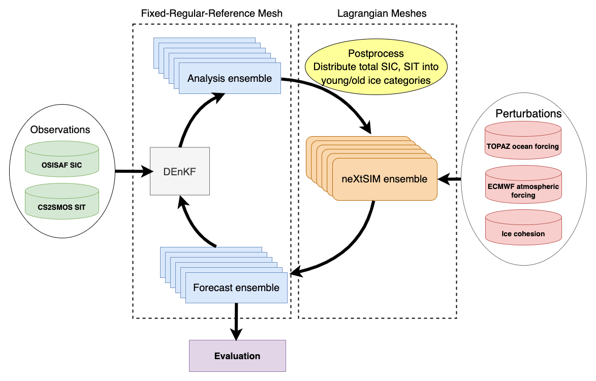
Figure 1Flowchart of the ensemble–DA platform. DEnKF: analysis step; neXtSIM: model forecast step; OSI-SAF SIC/CS2SMOS SIT observation: assimilated observations; TOPAZ forecasts and ECMWF forecasts: upstream forcing data for neXtSIM; field perturbations: see Sect. 4.1; fixed and regular reference mesh: forecast and analysis state variables are exchanged on a pre-defined regular mesh.
In this section, we describe the components of the ensemble–DA system: the ensemble perturbations, the statistical models of the observational errors (i.e., its error covariances), selected model states passed to the DA, and the analysis scheme (DEnKF). A schematic flowchart of the system is shown in Fig. 1.
4.1 Perturbations of atmosphere, ice, and ocean forcing
As a crucial component of the ensemble–DA system, the forecast ensemble is generated by neXtSIM through randomly perturbed atmospheric forcing and model parameters (ice cohesion in the present case), plus randomly perturbed oceanic forcing. The former two perturbations have been investigated in the Cheng et al. (2020) study, which shows that the modeled SID is less sensitive to the initial model state than to the atmospheric forcing applied throughout the run. In addition, uncertainties from the ocean processes (the TOPAZ4 data) are also considered in this study.
In the atmospheric forcing dataset, we perturb the horizontal 10 m wind velocities, the downward longwave radiation, and the snowfall rate that are considered to be dominant factors for a winter period. In the ocean forcing dataset, the SSS and SST are perturbed since they are known to impact SIC and SIT through thermodynamic processes. Using the same perturbation system as TOPAZ4 (Sakov et al., 2012), the perturbations are spatiotemporally correlated with a decorrelation timescale of 2 d and a horizontal decorrelation length scale of 250 km, with the random field generator introduced by Evensen (2003). The random perturbation fields have standard deviations of m s−1 for wind speed, W m−2 for the longwave radiation, 100 % for snowfall rate (using an unbiased lognormal distribution), 0.1 ∘C for SST, and 1 PSU (practical salinity unit) for the SSS. To limit the impact of SST on the ice formation around the ice edge, we multiply the SST perturbations by the open-water fraction in a grid cell. Following Sakov et al. (2012), the perturbations of horizontal wind velocities are derived from a surface-level pressure perturbation with a non-divergent constraint. The non-divergent constraint prevents the sea ice cover from breaking up excessively.
In addition to perturbing the upstream forcing dataset, the ice cohesion field is initialized as a heterogeneous random field following a uniform distribution between 20 and 40 kPa without spatial correlation (Cheng et al., 2020), which is different for each ensemble member. The cohesion field is kept constant unless a remeshing occurs, in which case the cohesion on the newly created model grid cells is given as the average of their nearest neighbors.
4.2 Observation uncertainties
The OSI-SAF SIC product provides an estimate of the instrument uncertainty to which we must add the related representation error (Janjić et al., 2018). The latter is notably challenging to evaluate and is usually computed based on pragmatic choices. Following Sakov et al. (2012), we estimate the total observation error variance (sensor and representation errors) as a function of SIC,
with c being the SIC. A visual comparison (not shown) between the error variances from Eq. (1) and those specified in OSI-SAF SIC confirms that they agree qualitatively but that Eq. (1) gives slightly higher uncertainties in certain areas as aimed for. Due to the difficulties of retrieving SIT from remote sensing, the uncertainty of the CS2SMOS SIT product is relatively high. The uncertainty contains the sensor errors, the inverse model representation error, diagnosed observation errors, and the bias (inconsistency) between the CryoSat-2 and SMOS observations. Instead of using the CS2SMOS built-in uncertainty, we define the observation error variance , referring to the empirical formula of Xie et al. (2018), as an increasing function of ice thickness hice:
The coefficients in Eq. (2) are fine-tuned based on a 3-year-long dataset of observations.
4.3 Multivariate analysis update
Previous studies have shown that multivariate DA can improve the SIT even when the SIC alone is assimilated (Massonnet et al., 2015; Zhang et al., 2018; Mu et al., 2020). Hence, in this study, the SIT and SIC are included among the updated state variables in the analysis steps. At least one state variable (either SIC or SIT) in our state vector has observations in the following DA experiments. Moreover, because the freezing and melting of sea ice are strongly driven by the ocean boundary conditions in winter, we also include the SSS and SST among the analyzed variables. Because SSS and SST are prognostic variables in the slab ocean of neXtSIM, this implies that the DEnKF shall adjust the ocean state variables following the change in sea ice via the cross-covariances of these analyzed variables. Nevertheless, in view of the simplicity of the slab ocean model, this does not constitute a truly coupled data assimilation setup; see Penny and Hamill (2017). To summarize, the state vectors for DA (i.e., the quantities to be updated at analysis steps) are absolute SIT, SIC, SST, and SSS.
Recall that neXtSIM includes the so-called effective SIT instead of the absolute SIT among its prognostic variables. To assimilate the observed absolute SIT, we would need to modify the observation operator to include the nonlinear mapping from the effective SIT to the absolute SIT. Instead, we opted to transform the effective SIT in the model output into the absolute SIT before applying assimilation. This choice allows for maintaining a linear observation operator in the DA algorithm.
As mentioned in Sect. 2.1, the model has three ice categories: open water, young ice, and old ice. Instead of using a multi-category update as in Massonnet et al. (2015), SIC and SIT in our state vector are both a sum of young and old ice, and we redistribute the analysis updates in the respective categories via a post-process whose details are given in Sect. 4.5.3.
4.4 Mapping model states onto the fixed and regular reference mesh
At the analysis steps, the state vector indicated in Sect. 4.3 is mapped from the individual Lagrangian mesh of the members onto a fixed and regular reference mesh. The fixed and regular reference mesh has a horizontal resolution of about 12 km over the Arctic Ocean, extracted from the global tripolar grid with a 0.25∘ resolution, referred to as ORCA-R025 (Bernard et al., 2006). The mapping is accomplished by a bilinear interpolation. The analysis state vector is then interpolated back to the corresponding Lagrangian mesh of the ensemble members for the subsequent forecast step following Aydoğdu et al. (2019). Once the updated values of the physical quantities in the state vectors are projected back on each member's mesh, they evolve with the forecast run in which the Lagrangian meshes move according to the ice velocity fields.
4.5 The deterministic ensemble Kalman filter (DEnKF)
We use the DEnKF (Sakov and Oke, 2008) to assimilate the SIT and SIC observations. Unlike the stochastic EnKF, the DEnKF does not require the observations to be perturbed to avoid filter divergence. DEnKF is also conceptually more straightforward compared to other transform-based deterministic EnKFs (see Carrassi et al., 2018, for the differences between various EnKF flavors). The open-source DA software, EnKF-C version 2.8.0 (Sakov, 2014), is adopted to perform the DA. The EnKF-C provides the functionality for automated quality control as well as ensemble inflation and localization, which are briefly outlined below.
4.5.1 Preprocessing and quality control
EnKF-C provides a toolbox to preprocess and perform observation quality control. Observations within our model domain are selected and interpolated onto the fixed and regular reference mesh (see Sect.4.4) by its built-in operator. Additionally, observations within 50 km of the coastline are removed to avoid spurious effects known to be present in these satellite-derived products near the coasts.
When the forecast and observation uncertainties do not overlap (i.e., innovations larger than expected by the EnKF), the assimilation responds by giving large analysis increments, which may cause model imbalances in the subsequent forecast run. To reduce the impact of those large innovations, EnKF-C uses an adaptive quality control method introduced by Sakov and Sandery (2017) and artificially inflates the observation variance by an adjustable K factor without removing the observations. The effect of this adaptive quality control method has been studied in Sandery et al. (2020, Fig. 1) by comparing the original and modified observation error spread. In the case of severe model biases, K can be set to 1, while in our case, as demonstrated by the free run in Williams et al. (2021), we do not expect severe bias in neXtSIM and found that the default value K = 2 maintains adequate analysis ensemble spread.
4.5.2 Inflation and localization
Idealized studies by Zhang et al. (2018) show that inflation and localization are necessary to improve sea ice forecast in the DA cycles. To correct the underestimation of sample variances, covariance inflation can be introduced in a multiplicative way (e.g., Anderson and Anderson, 1999; Anderson, 2007; Anderson et al., 2009). Inflating the observation variance can reduce the observation effect in DA and thus maintain the spread from the ensemble forecast. However, the Arctic has very variable observation coverage. Some interior regions have very sparse observations, while some model variables are not directly observed. In such areas and for these variables, multiplicative covariance inflation will inflate the ensemble anomalies and spread exponentially, which also amplifies the biases in the observed variables in the case of multivariate assimilation. An alternative use of inflation is to act only where observations are assimilated (Sakov et al., 2012; Xie et al., 2017). The DEnKF includes a kind of additive inflation by its algorithm construction, explained in Sect. 3, as well as the R-factor inflation of the anomaly update (Sakov and Oke, 2008). We also draw attention to the point that in our experiments, besides errors in the forcing, we have model errors that are sometimes omitted in the literature and compensated for by multiplicative inflation. We believe that explicit stochastic model errors are preferable and make more physical sense (e.g., Scheffler et al., 2022). Moreover, in our experiment, both the atmosphere and ocean forcings are perturbed throughout the simulation, maintaining an ensemble spread for our DA system. This partially allows us to avoid additional multiplicative inflation.
Therefore, we intentionally multiply the observation variance for all observations by a factor of 2, but we do not use any other multiplicative inflation. Following Sakov et al. (2012), we use a localization radius of 300 km for sampling both SIC and SIT observations. This corresponds to an effective e½-folding radius of about 90 km.
4.5.3 Post-processing of nonphysical analyses
As stated in Sect. 4.3, we simultaneously update the SIC, SIT, SST, and SSS by the DEnKF. The important, albeit generally nonlinear, ocean and sea ice interactions might not be fully captured by the error covariances that in turn determine the DEnKF updates, resulting in nonphysical model states. To mitigate this potential issue, we apply a sequence of post-processing steps as follows. Firstly, as a sanity check, the ocean variables are capped by the SSS between 5 and 41 PSU and the SST between the freezing point and 35 ∘C, far away from reasonable values. Secondly, the post-processing handles the analysis update of the total SIC. To remove the effect of unreliable observations, SIC is set to zero wherever the analysis SIC 15 % and SIC is capped by 100 %. We assume the model uncertainty of SIC arises mainly from the young ice. Hence, the SIC increment, which is the difference between the analysis and the background total SIC, is first applied to update the young ice. The SIC of young ice is capped by 100 % in the case of a positive increment. If the young ice is completely removed by a negative increment, the rest of the negative increment is removed from the old ice. If SIC is removed altogether, SIT, ridge ratio, and snow depth are all set to 0 for a no-ice situation.
After processing the SIC increment, we make a selective update for SIT. In the experiments wherein SIT is assimilated, the SIT in the entire domain is updated by the analysis. On the other hand, if only the SIC is assimilated, the SIT updated by multivariate covariances is applied in a limited region where the analysis SIC 90 %. This is done to remove possible unrealistic multivariate updates of SIT in the pack ice; high SIC values reaching the upper bound of 100 % do not fit the Gaussian assumption and sometimes lead to problematic bivariate error covariances with SIT. Our selection relieves the problematic updates in the DEnKF but retains the multivariate assimilation for intermediate SIC values. Then, the SIT of young ice and old ice is redistributed proportionally to the analysis fractions of young and old SIC. For “new” ice added by data assimilation, we assign 0.25 m SIT to the young ice and keep the old ice at zero. If the updated SIT of either young ice or old ice falls thinner than 0.01 m, we remove that category by setting the relevant ice quantities to zero.
These updated sea ice quantities then go through a final consistency check to be used in the model run. Young ice SIT and snow depth, in particular, are proportionally reduced if the SIC needs to be reduced from over 100 %, in which case the reduction is applied only to young ice SIC. The internal ice temperature of new ice is updated based on the updated SIT, SIC, snow thickness, and water-freezing temperature. Internal ice temperature must be at the freezing point for regions without old ice. For open-water areas without any ice, the consistency check ensures the SIT, SIC, and snow depth are all zero for both ice categories with the freezing point temperature of water. Similarly, for young ice areas, the SIT, SIC, and snow depth of old ice are all zero, and ice temperature is at the freezing point of ice salinity.
We carry out four ensemble–DA experiments to investigate the impact of different observation products and assimilation frequencies. Details are summarized in Table 1 together with a free ensemble run for reference.
In particular, in two of the experiments, hereafter referred to as SIC7 and SIT7, we assimilate observations of only one quantity, either SIC or SIT, respectively, with the last digit indicating the weekly DA frequency. These experiments are intended to reveal the effect of multivariate assimilation on the observed and non-observed sea ice variables. Similar to previous studies (see, e.g., Xie et al., 2018), we investigate the joint assimilation of both SIC and SIT in two further experiments. In experiment SIC7–SIT7, we assimilate SIC and SIT simultaneously on a weekly cycle. Recalling that the SST and SSS in the slab ocean component of neXtSIM are nudged towards the daily ocean surface forcing of TOPAZ4 with the relaxation timescales set as 5 d (see Sect. 2.2), the SST and SSS updated by weekly multivariate analysis are gradually “overwritten” in neXtSIM by the TOPAZ4 values. Hence, we increase the assimilation frequency and conduct the additional experiment SIC1–SIT7, whereby SIC is assimilated daily and SIT is assimilated weekly, following the satellite data availability. In this experiment, the effect of ocean nudging should be mitigated and the impact of SIC observations intensified. Moreover, the higher observational frequency may damp the nonlinearity in the error evolution in subsequent analyses, potentially avoiding the violation of the Gaussian assumption at the basis of the DEnKF (see Bocquet and Carrassi, 2017, for a discussion on the effect of observation frequency and accuracy on the error evolution). Naturally, the downside of high-frequency assimilation is the increased computational cost (Lange and Craig, 2014; He et al., 2020). More frequent assimilation of SIT was not considered in view of the limited daily coverage of CryoSat-2 data in the ice pack. As a reference, we produce a free ensemble experiment without DA constraints, referred to as the free run hereafter.
Because the CS2SMOS product is only available in the ice-freezing season, all the experiments are conducted from 18 October 2019 to 16 April 2020 (182 d). The initial conditions of the experiments are generated from an ensemble spin-up run from 3 September to 17 October 2019 (45 d). The spin-up run is initialized from the neXtSIM-F forecasts (Williams et al., 2021) and integrated with different perturbations for each ensemble member as described in Sect. 4.1. All the DA experiments and the spin-up run use 40 ensemble members. The ensemble size is chosen after evaluating the spread of a larger free-run ensemble of 100 members during the spin-up period, noticing that the spread becomes almost insensitive to the ensemble size when the latter exceeds 40. This behavior is typical of deterministic EnKF such as the DEnKF adopted here (see Carrassi et al., 2022).
Table 1Summary of the ensemble experiments. For all the experiments, the simulation period is from 18 October 2019 to 16 April 2020, and the ensemble size is 40.
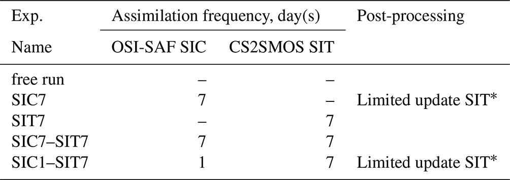
∗ When only SIC is assimilated, SIT in the model is updated with analysis SIT only if the analysis SIC 90 % – see Sect. 4.5.3.
In this section, we present the results from the model forecasts of the experiments in Table 1 from 18 October 2019 to 16 April 2020, validated by the observations before the sea ice variables are assimilated. Although assimilated into the experiments, the CS2SMOS SIT and OSISAF SIC observations are used in the validation of model forecasts before each assimilation step with the awareness of potential dependency. Independent validation is also performed using the OSISAF SID observations. The section is structured to show results for different quantities: SIC and SIE in Sect. 6.2, SIT in Sect. 6.3, and SID in Sect. 6.4.
6.1 Definition of metrics and overall performances
We use several metrics to validate the ensemble forecasts against the observations, thus evaluating the forecast skills of our system. All metrics are defined in observation space, i.e., in the observation grid onto which the model states are interpolated.
Bias and root mean square difference (RMSD) between the ensemble mean and the observations are utilized to assess the forecast skill, the definitions of which follow Williams et al. (2021). For a scalar variable field, such as SIC and SIT, the ensemble mean vector at time t is defined as , where x(t)∈ℝm, m is the vector length, n is the ensemble size, is a matrix containing the ensemble members along its columns, and . The bias of a scalar variable is – contrary to the innovations – defined as model-minus-observations , where the operator 〈⋅〉 represents the spatial average of over ice-presented pixels, y(t)∈ℝo is the observation vector, and ℋ is the observation operator mapping from model states with two sea ice categories to the observations of total SIC and total absolute SIT on the observation grid. In our analysis, we define a “robust” bias by removing grid points outside the [2 %, 98 %] quantiles of bias on the domain. This makes with .
The RMSD is defined as , where is the Euclidean norm, with outliers removed. We also compute the temporal average of the bias over the time period [t1,t2], which is .
For vector quantities such as the SID, the vector of the ensemble mean at time t is defined as , where x1(t) and x2(t)∈ℝm represent the two horizontal orthogonal components, is the ensemble matrix with the first m rows representing the first orthogonal component of the quantity, the rest of the m rows represent the second orthogonal component, and . The relevant observation vector has o number of observations with its horizontal orthogonal components y1(t) and y2(t)∈ℝo. The spatially averaged bias of a vector variable can be defined as the error of the magnitude of speed: . RMSD is the error in speed , where |⋅| is defined as , where ∘ is a component-wise product, with being the vector component-wise square root. In the vector case, the outliers are not removed. We also compute the vector RMSD (VRMSD), , which accounts for errors in speed and direction. Note that the metrics defined above follow Williams et al. (2021) with adjustments for ensembles.
We evaluate the SIE by adopting the integrated ice-edge error (IEEE, Goessling et al., 2016) and the spatial probability score (SPS, Goessling and Jung, 2018). The IIEE indicates the mismatch of SIE between the model outputs and observations usually occurring around the sea ice edge, which is designed to evaluate deterministic forecasts. Moreover, the IIEE can easily be decomposed into overestimation and underestimation of SIE. Using the ensemble mean, we compute the IIEE overestimated and underestimated components, O and U. The SPS is an extension of the IIEE for ensemble forecasts. However, the SPS does not provide information on overestimation or underestimation. Hence, we utilize both metrics in the SIE assessment. Formulas of the relevant metrics can be written as
where A is the area of the model domain, and c(x) is a sea ice indicator function such that c(x)=1 for x>15 %; otherwise, c(x)=0, where x represents ice concentration, and the subscripts o and f stand for the observed and forecast concentrations, respectively, while indicates the ensemble mean of the overall SIC forecast in the observation space. Note that only the 15 % concentration isoline is used by the IIEE and a large share of the concentration information is not taken into account. Finally,
where P is the ensemble probability of SIE of each model grid point.
Before discussing the skills in each of the considered variables in detail, we summarize their performances by providing the grid-weighted spatial and temporal averages of the bias, RMSD, and VRMSD in Table 2. The best result per variable and metric is highlighted in bold.
Table 2Summary of the metrics for SIC, SIT, and SID: spatiotemporal averaged bias, RMSD, and VRMSD among the experiments. SIC is validated against OSI-SAF SIC, SIT is validated against CS2SMOS SIT, and SID is validated against OSI-SAF SID. The best value of each ice feature among the experiments is bolded.

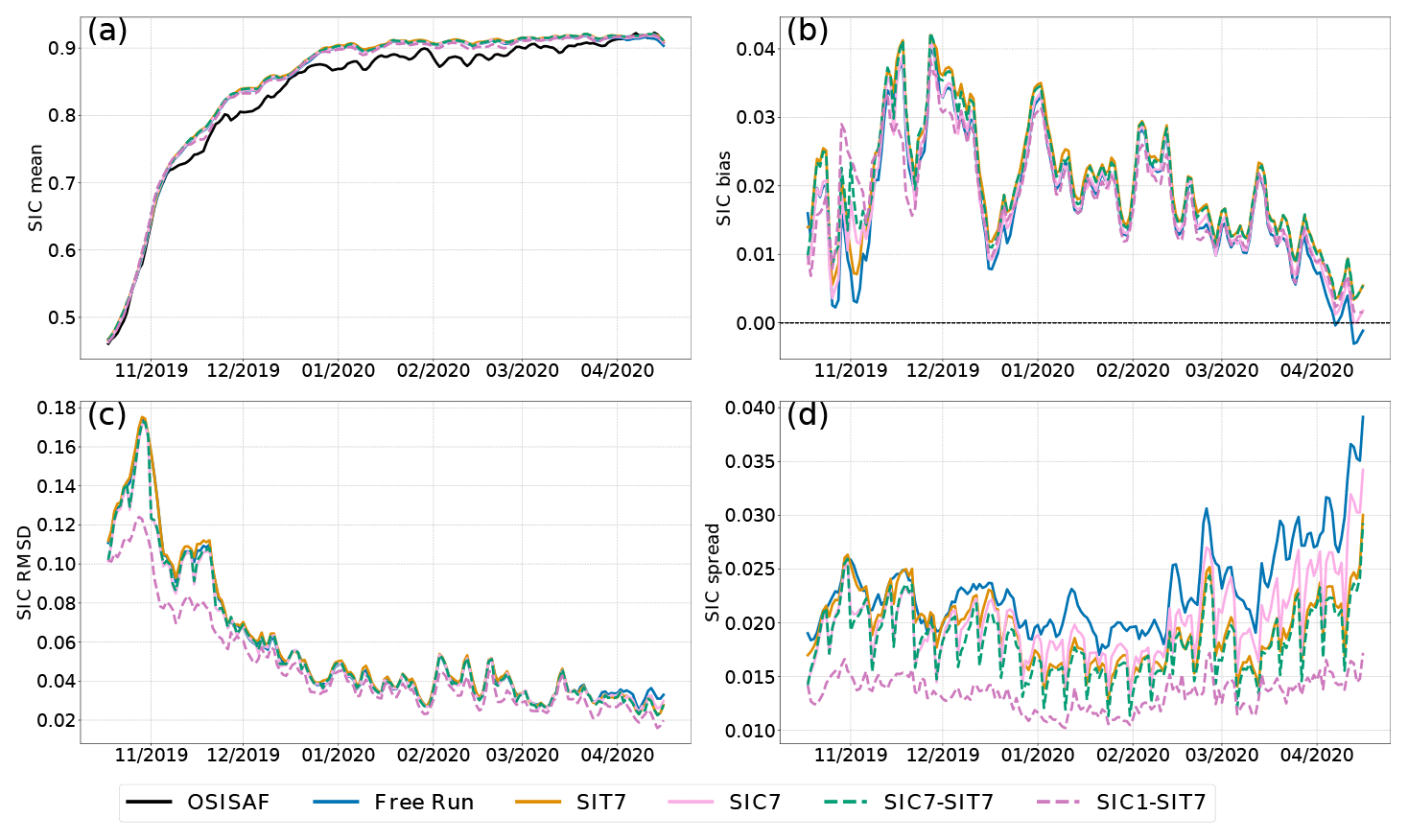
Figure 2Time series of spatially averaged SIC from the model forecast against OSI-SAF SIC from 18 October 2019 to 16 April 2020. (a) Ensemble mean SIC; (b) bias; (c) RMSD; (d) ensemble spread (standard deviation).
6.2 Evaluation of sea ice concentration and extent
Figure 2a shows the temporal evolution of the area-weighted average of the ensemble mean SIC from the experiments in Table 1. The black curve indicates the OSI-SAF SIC observations. All experiments capture the observed increase in SIC well. Nevertheless, although the free run is almost indistinguishable from all the DA experiments, it shows a slight overestimation from November onwards. Among the DA runs, experiment SIC1–SIT7 (dashed purple line) shows marginally better agreement with the observations than the others.
Figure 2b and c display the time series of bias and RMSD of SIC, respectively. Overall, all the experiments show excess sea ice with minor differences. The SIC bias is generally smaller when SIC is assimilated, as expected. The experiment with daily SIC observations, SIC1–SIT7, generally gives the smallest biases. We see, however, that the free run has the smallest bias in the first weeks, occasionally in December 2019 and April 2020. The free run also shows the (slightly) smallest average bias of 0.014 (see Table 2). This undesired, albeit small, increase in bias in the DA experiments is due to the asymmetric effect of DA in the cases of local overestimation and underestimation. We shall clarify this further when discussing Fig. 5 later.
In contrast to the bias, we see an obvious impact of DA on the RMSD (panel c). In particular, SIC1–SIT7 shows the lowest RMSD consistently throughout the whole period (average value of 0.027 in Table 2). This is a notable reduction compared to the other experiments, which show very similar values. The RMSD decreases mostly during fall 2019 (a relative reduction of up to 27 %) and then oscillates during spring 2020. The effect of DA becomes smaller after January 2020 when the sea ice covers the majority of the Arctic Ocean (see the increase in SIC in Fig. 2a), and there is not much room for action.
The DEnKF estimates the uncertainty via the ensemble spread, a flow-dependent proxy for the forecast error standard deviation. Comparing the spread of ensemble–DA experiments with the free run provides an estimate of how much uncertainty is reduced by the DA. We show the time series of the ensemble spread from all the experiments in Fig. 2d. All experiments maintain a stable spread except for an increase caused by the seasonal ice melt since mid-March 2020; the assimilation reduces the ensemble spread compared to the free run, although to a different degree depending on the experiment. In the experiments with weekly assimilation of either SIT or SIC, the spread decreases significantly after 1 d forecasts from the analysis. However, it then quickly builds up during the 2 following days of forecasts, reaching levels close to the free run from October 2019 to January 2020, showing that the assimilation of SIC has a short memory compared to the assimilation window. The weekly assimilation of SIC is slightly more efficient from April onwards, consistent with Lisæter et al. (2003). However, only the daily SIC assimilation experiment can efficiently reduce the SIC errors, SIC1–SIT7, showing a relatively smaller spread across the full period. Both spread and RMSD are reduced by about 0.005. Importantly, these results show that thanks to the continuous perturbations applied to the external forcing, the ensemble system can maintain spread even in the winter when the system's internal variability is tiny.
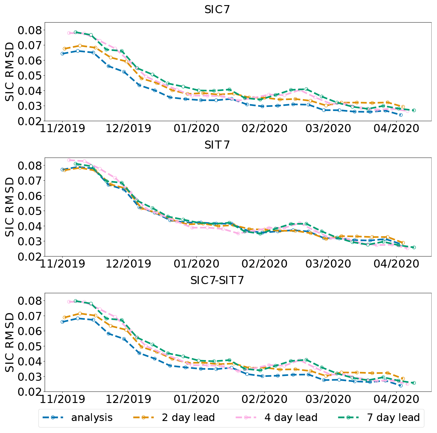
Figure 3SIC RMSD for 4 weeks of the moving-averaged forecast regarding the assimilation time. Each line represents a different lead time.
To get a clearer picture of the improvements in the SIC forecast skill by weekly assimilation, we present the SIC RMSD from the perspective of the lead time in Fig. 3. Each curve represents the temporal evolution of the moving average in a 4-week window of the analysis and forecast error after 2, 4, and 7 d of lead time. The clustering and spread of the curves at a specific time (viewing vertically) indicate the growing forecast error with the increased lead time: we observe that both SIC7 (top row) and SIC7–SIT7 (bottom row) show clear growth of the RMSD with increasing lead time, while the forecast errors are independent of lead time in SIT7 (middle row). This is a result of the reduction of model error in the analysis (after lead day 7) in SIC7 and SIC7–SIT7 with increasing error in the subsequent model forecast (in lead day 1), which is not reflected in the daily averaged time series in Fig. 2. We observe that the errors saturate in a range of 2 to 7 forecast lead days depending on periods, which we attribute to the variability of weather conditions. This highlights the improvements in the analysis due to the assimilation of SIC but also reveals that the multivariate assimilation of SIT has little influence on SIC. With the decreasing SIC RMSD over time (viewing horizontally), the forecast errors among different lead times become similar to each other, showing the reduced effect of the assimilation on the forecast in the winter season.
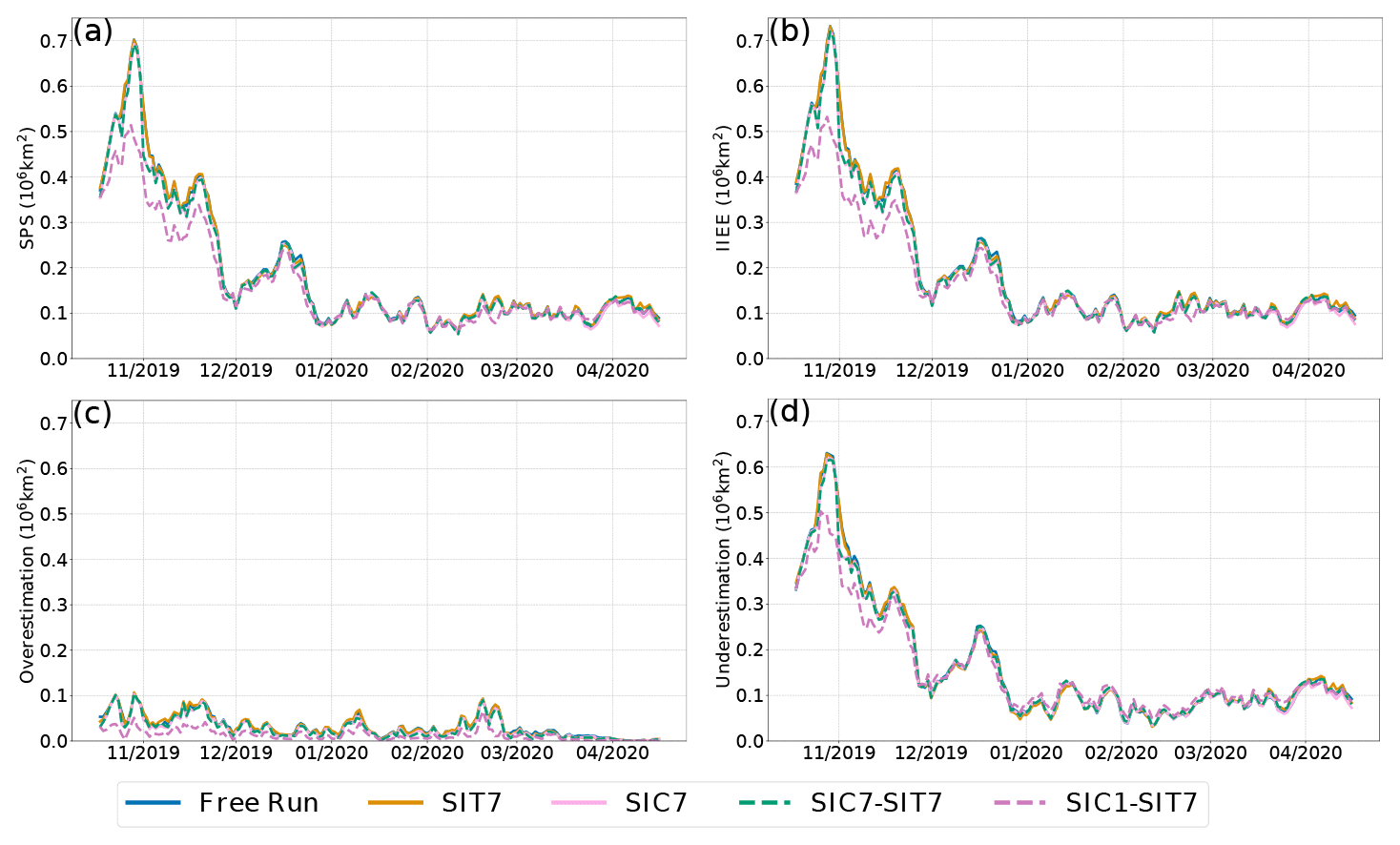
Figure 4Metrics of sea ice extent validated against OSI-SAF SIC over time. (a) Spatial probability score (SPS) is calculated using the full ensemble forecasts. (b) Integrated ice-edge error (IIEE) is calculated using the ensemble means and split between its overestimation and underestimation components in panels (c, d), respectively, which indicate the amounts of overestimation and underestimation in modeled SIE from the observations.
The SIE is also evaluated against the OSI-SAF SIC product from a domain-integrated view of the SIC. Figure 4 shows the time series of the (a) SPS, (b) IIEE, (c) overestimated component of IIEE, and (d) underestimated component of IIEE (see Sect. 6.1). The SPS and IIEE are almost identical for all runs. It is typical of a “healthy” ensemble that the ensemble forecasts and the observations are statistically indistinguishable. The SPS and IIEE behave similarly to the SIC RMSD (see Fig. 2c), which decreases to a steady state around January 2020 with small and rapid variations afterward. The overestimated and underestimated components of IEEE based on the ensemble mean give a different view of the bias of SIE in the ensemble mean forecasts: the SIE is primarily underestimated comparing Fig. 4c and d, which seems counterintuitive when the biases were showing a general overestimation of SIC. The discrepancy is likely caused by local underestimated SIC in the Beaufort Sea versus general overestimation over the Arctic, which will be further reviewed in Fig. 5.
The improvement of SIE due to DA is most visible in SIC1–SIT7 compared to the others, highlighting the importance of frequent SIC assimilation. The underestimated component of the IIEE is improved in the first months only, consistent with the impossibility of adding more ice in a fully packed Arctic. In contrast, the overestimation is improved throughout the whole period due to the more frequent (daily) assimilation of SIC. In absolute IIEE numbers, the impact of assimilation is mostly on reducing underestimation, while in relative terms, the overestimation may seem easier to correct with daily assimilation.
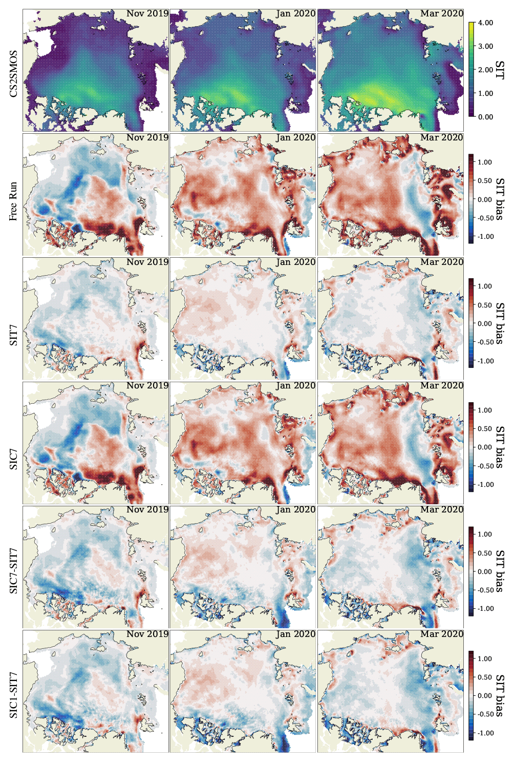
Figure 5Monthly average of SIC observations (first row) and SIC bias between the model forecasts and the OSI-SAF SIC product. Panels from left to right are November 2019, January, and March 2020. Red and green lines are the sea ice edges (applying the classical threshold of 15 % SIC) from the observations and the ensemble mean forecasts.
To further demonstrate the effect of DA, Fig. 5 shows the spatial distribution of the monthly SIC average bias in selected months, representative of the SIC evolution. The top row displays the observed SIC, and the SIC biases from the different experiments are then shown below. The distribution of SIC bias is similar in all experiments, showing an overall positive bias in the ice pack where concentrations are high (>80 %). High-bias regions are also located near the marginal ice zone, in coastal seas, and east of Greenland. The SIC bias in the marginal seas is visibly reduced in SIC1–SIT7 compared to the free run and the other DA experiments, among which there are no noticeable differences. These results agree with the time series of bias and RMSD of SIC and SIE shown in Figs. 2 and 4.
The figure offers a resolution of the apparent contradiction between the overestimated SIC bias and the underestimation-dominated IIEE decomposition: all experiments generally predict smaller SIE (green curves) compared to the observation (red curves) near the open-water boundaries. This then causes the predominant underestimation of SIE seen in Fig. 4, but within the 15 % isoline, most of the biases are positive, summing up to a positive SIC bias in Fig. 2. In November 2019 (left column), the large bias in the Beaufort and Chukchi seas and the Kara Sea contributed to most of the SIC RMSD seen in Fig. 2. As the sea ice freezes gradually, the SIC bias disappears as the ice expands to the Bering Strait and the Siberian coasts. Meanwhile, the SIE bias decreases over time, as the SPS and IIEE indicate. Disagreements between modeled and observed SIC and SIE remain in the Nordic seas: the Greenland Sea, the Barents Sea, and the Kara Sea in January and March 2020, which are only slightly affected by the assimilation and likely biased towards their ocean boundary condition. The delayed ice growth in the model is mainly related to the warm ocean condition from TOPAZ4 since the atmosphere temperature is commonly below the freezing point. Because the SIC and SIE evolution primarily depends on the underlying ocean boundary condition, we argue that during the model forecast, the daily TOPAZ4 data counteract the effect of weekly assimilation on the ocean states. This is not the case in SIC1–SIT7, which updates the analysis SST and SSS daily in the slab ocean via DA. This argument is in agreement with the study by Williams et al. (2021), which blamed the model for the underestimation due to the lack of input of detached landfast ice and fast melting in the seas. This phenomenon is further discussed in Sect. 7.
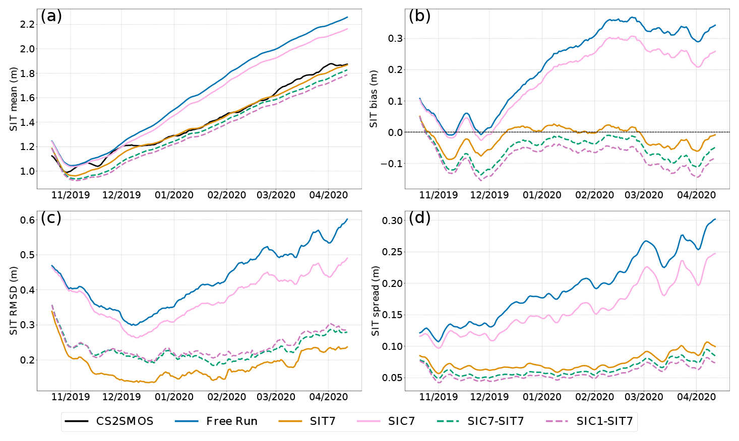
Figure 6Time series of spatially averaged SIT from the model forecast against CS2SMOS from 18 October 2019 to 16 April 2020. (a) Ensemble mean SIT; (b) bias; (c) RMSD; (d) ensemble spread (standard deviation).
6.3 Evaluation of sea ice thickness
We now examine the SIT forecast skill of our experiments. Similar to Fig. 2, Fig. 6 shows the (a) spatial mean, (b) bias, (c) RMSD, and (d) ensemble spread of SIT validated against the CS2SMOS SIT product. We can see that all experiments capture the mean SIT evolution in the measurements. In particular, they track the SIT increase after a short period of decrease in October 2019. Nevertheless, the free run and SIC7 significantly overestimate the mean SIT (see also panel b) from December 2019. It is worth mentioning that, thanks to the multivariate assimilation of SIC, experiment SIC7 is slightly better than the free run. As expected, all the experiments in which SIT is assimilated show, in general, much better skill in predicting SIT. Nevertheless, we also observe a counterintuitive impact of assimilating both SIC and SIT (i.e., experiments SIC1–SIT7 and SIC7–SIT7), yielding poorer SIT than when assimilating SIT alone. The differences among the DA experiments are more evident in the bias (panel b) and the RMSD (panel c).
The free run shows the largest positive bias and RMSD of SIT over time. Errors are reduced by all DA experiments, with SIC7 being the least effective; see also Table 2. Experiment SIT7 gives the lowest bias (close to zero) and the smallest RMSD: the spatiotemporal averages for the bias and the RMSD are −0.051 m and 0.118 m, respectively (see Table 2). SIC7–SIT7 and SIC1–SIT7 show relatively larger RMSD and similarly larger negative bias than SIT7. We also note that assimilating SIC daily (experiment SIC1–SIT7) gives both larger bias and RMSD than assimilating SIC weekly (experiment SIC7–SIT7). The time-averaged bias and RMSD (see Table 2) are −0.113 and 0.173 m for SIC1–SIT7 and −0.09 and 0.155 m for SIC7–SIT7, respectively. Although this degradation seems to contradict the positive impact of SIC7 over the free run, we believe that the slight reduction in SIT prediction skill is caused by artifacts of the DEnKF update applied to SIT and SIC, whereas the relationship between the two variables is nonlinear. A practical remediation would be to attenuate the effect of SIC observations on SIT analysis. We will discuss this in Sect. 7. In contrast to the similar SIC spread in Fig. 2d, the SIT spread in Fig. 6d exhibits two groups. The top lines show a large increase in the SIT spreads in experiment SIC7 and the free run without SIT assimilation. The unconstrained free run shows the largest spread, which is slightly reduced in SIC7. In the lower lines, all the experiments assimilating SIT show much smaller spreads with a slower increase toward the end of the simulation period. SIC1–SIT7 shows the lowest spread, slightly smaller than all other experiments. We attribute this behavior to the lower variability of the SIT that is constrained by the assimilation of SIT data.
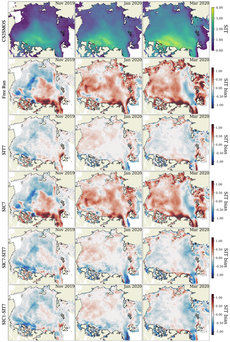
Figure 7Same as Fig. 5 but for monthly averaged SIT bias between the ensemble runs and the CS2SMOS SIT product.
Figure 7 shows spatial maps of the monthly average of the SIT bias against CS2SMOS SIT data in November 2019, January 2020, and March 2020, from left to right. The first row of panels shows the observed SIT, while the others present the bias of the different experiments. The time evolution of the bias pattern (from November 2019 to March 2020) depends on the different assimilation strategies. The free run has a negative SIT bias in November 2019 up to about 1 m mainly in the Beaufort and Chukchi seas, the East Siberian Sea, the Laptev Sea, and the Kara Sea. It also shows that the positive bias is predominant in the rest of the Arctic, especially in the Canadian Archipelago and the northern coast of Greenland (>1 m). In January and March 2020, the positive bias is predominant in the Arctic region except for the band of negative bias from the Nansen Basin and the Laptev Sea occurring in March 2020. SIT is overestimated near the coast all over the Arctic, indicating too much ice ridging in the model. SIC7 shows slightly reduced SIT bias from the free run due to the multivariate assimilation of SIC, as discussed in Fig. 6. In line with the results in Fig. 6, SIT7 has the smallest bias. In particular, SIT7 successfully reduces most of the large SIT bias in the Canadian Archipelago and the Greenland, Barents, and Kara seas found in the other experiments. The remaining SIT bias in SIT7 appears to be concentrated near the coasts and ice edges. This is because of no DA applied within 50 km coast zones and the high SIT uncertainty in the CS2SMOS data. By assimilating SIC and SIT observations, SIC7–SIT7 shows a similar pattern as SIT7 but a more pronounced negative bias. The bias patterns of SIC1–SIT7 and SIC7–SIT7 are similar overall, implying the weak influence of assimilating SIC on SIT again.
6.4 Evaluation of sea ice drift
The drift of the sea ice, including its directions and speed, is important for both operational forecasts and atmosphere–ice–ocean interactions. The main physical mechanisms of sea ice drift are the wind drag at the sea ice surface and the internal sea ice forces. We are thus interested in assessing how our DA-based predictions reproduce the observed SID: this is validated using the OSI-SAF SID product, which is not assimilated in our experiments.
The free run can already reproduce the observed drift variations without DA. This makes it challenging for DA to bring visible improvements (Williams et al., 2021). From the spatiotemporally averaged metrics in Table 2, the bias in SIC7–SIT7 is the lowest with 1.279 km per 2 d. The VRMSD values in the SIT assimilation runs are similar with obviously the lowest error compared to other runs. SIT7 has the best VRMSD of 7.099 km per 2 d, which is slightly smaller than SIC7–SIT7 (7.13 km per 2 d) and SIC1–SIT7 (7.115 km per 2 d). In contrast, the smallest RMSD is from SIC7 at 4.21 km per 2 d and the free run, outperforming experiments with SIT assimilation. Overall, we observe small improvements in the modeled SID when we assimilate SIT.
We propose an ensemble-based data assimilation system for the Lagrangian sea ice model, neXtSIM, to enhance its Arctic sea ice forecast skill. The DEnKF is applied to work with a time-dependent, non-conservative model mesh, following the projected EnKF strategy introduced by Aydoğdu et al. (2019). The Lagrangian nature of the model implies that each ensemble member evolves on an independent adaptive moving mesh. At analysis times, we interpolate the ensemble members onto a fixed and regular reference mesh, on which the analysis is carried out. The analysis state variables are then projected back to the individual member meshes. The ensemble is generated by perturbing an internal model parameter and external forcings, namely the ice cohesion, the atmospheric forcing (10 m wind velocities, longwave downwelling radiation, and snowfall rate) from the ECMWF product, and the oceanographic forcing (SST, SSS) from the TOPAZ4 forecast. The system assimilates satellite-based sea ice products (CS2SMOS SIT and OSI-SAF SIC) and updates the state vector variables SIC, SIT, SSS, and SST by DEnKF. The model decomposes the sea ice into age categories, but the analysis is performed on the total ice. Therefore, empirical post-processing steps are introduced to redistribute the analysis of sea ice states into young and old categories and avoid imbalances caused by nonphysical updates.
Ensemble–DA experiments are carried out from October 2019 to April 2020 (Table 1) with different assimilation strategies. The results show that the forecast skill of sea ice improves and benefits from the assimilation. The forecast skills of SIC and SIE are the best in the SIC1–SIT7 experiment with daily assimilation of SIC (Figs. 2 and 4). The daily assimilation reduces the model uncertainties, e.g., in the SIC RMSD (Fig. 2) and spread (Fig. 3). The underestimation of SIE is reduced in the Beaufort–Chukchi Sea and the Kara–Barents Sea in SIC1–SIT7 (Fig. 5). The IIEE is roughly comparable to those obtained by the operational TOPAZ4 system, with a large part of the errors caused by underestimation (see the validation time series for sea ice at https://cmems.met.no/ARC-MFC/V2Validation/timeSeriesResults/year-day-01/SItimeSeries_year-day-01.html#OSI_xIIEE, last access: 12 August 2022). The similarities of IIEE results are thus likely caused by areas of ocean surface temperatures that are too warm. Nevertheless, we also note that the IIEE may contradict the SIC statistics since it only uses an isoline of the SIC. Moreover, we observe a large reduction of the (both positive and negative) model SIT biases by assimilating the CS2SMOS SIT data (Sect. 6.3). Specifically, experiment SIT7 cuts the model SIT bias to almost zero, and its corresponding RMSD is the lowest among all experiments. The SIT errors are also reduced in the joint SIC–SIT assimilation experiments, although to a lesser extent; this implies that the apparent benefit of multivariate DA becomes detrimental when assimilating both SIT and SIC, which is further discussed later. Furthermore, small improvements on SIT are visible when assimilating SIC only, SIT7, which agrees with the small effects from multivariate DA found in the data assimilation framework of the coupled ocean–ice model, ROMS-CICE (Fritzner et al., 2019). Although the improvements on the SID are less apparent, the model performs on par with the earlier results with direct insertion (Williams et al., 2021) and outperforms the TOPAZ system using an older sea ice rheology and the DEnKF.
Three points in the results are further discussed as follows: firstly, assimilating SIC in the joint SIC–SIT assimilation experiments (SIC1–SIC7 and SIC7–SIT7) causes more negative SIT bias than in the SIT7, which assimilates only SIT (see Figs. 6 and 7). This undesired effect arguably comes from inadequate cross SIT–SIC error covariance in the DEnKF. The modeled SIC and SIT are generally positively correlated in the ensemble (not shown), especially when forming new ice at the ice edge. Given that the OSI-SAF SIC data are systematically lower than the model in most of the Arctic (see Fig. 5), this generally positive SIC–SIT correlation implies that the analyzed thickness is also generally thinner after SIC assimilation. Consequently, the SIC assimilation tends to transfer the bias to the SIT. The influences of SIT–SIC cross-covariance get naturally stronger with more frequent DA in SIC1–SIT7 compared with SIC7–SIT7 (see Figs. 6 and 7), leading to a stronger underestimation of SIT. This deterioration contradicts the case when SIC alone is assimilated and improves the SIT over the free run, but these improvements were most visible near the ice edge (see Fig. 7) where the SIT–SIC covariance is more linear and because a correct location of the ice edge indirectly improves the thickness of newly formed ice.
The second point concerns a challenge inherent to ensemble–DA methods. The observed–unobserved variables in the sea ice are often nonlinearly related. This limits the efficacy of the EnKF schemes, particularly for small ensemble size (e.g., Kimmritz et al., 2018). In our experiments, an issue is that both SIT and SIC are bounded variables (positive and less than 1 for SIC) and thus clearly non-Gaussian. Furthermore, by virtue of the two sea ice categories in the model, the local relationship between the modeled SIT and SIC is often nonlinear. To mitigate the impact of wrongly computed analysis corrections, we intentionally limited the SIT update to regions where SIC <90 % (see Sect. 4.5.3). As a side effect, it could reduce the impact of SIC7 on the SIT prediction. Moreover, previous literature agrees that the influence of assimilating SIC on SIE is significant but the influence on SIT is diverse. Most studies demonstrated that SIC assimilation only slightly affects SIT (Sakov et al., 2012; Zhang et al., 2018; Kimmritz et al., 2018). Mathiot et al. (2012) observed SIC improvement by combining the SIC and ice freeboard assimilation using EnKF, but mostly thanks to the ice freeboard assimilation. Tietsche et al. (2013) improved the spatial mean SIT by assimilating SIC and introducing mean thickness analysis updates, proportional to SIC. Moreover, Zhang et al. (2021) found that SIC assimilation causes SIT degradation in the GFDL (Geophysical Fluid Dynamics Laboratory) seasonal prediction system.
Thirdly, DA effectively reduces the uncertainty of the quantities directly observed in practice when, e.g., SIT or SIC is the sole observable. However, this benefit of DA is less pronounced when multi-variables are jointly assimilated. For example, assimilating SIT alone, SIT7 cuts the SIT bias by 61 % over the free run. In comparison, the improvement in the SIT bias by jointly assimilating SIC and SIT is smaller. Specifically, the bias is reduced by 49 % in SIC7–SIT7 and 43 % in SIC1–SIC7 from the free run. This reduction has been a well-known effect since the early days of data assimilation in weather forecasting: when more terms are introduced in a cost function, the optimal solution becomes the best compromise and fits each term less closely individually. So in our case, the SIT and SIC observations compete with each other, and the joint assimilation performs somewhat more poorly than the assimilation of the SIT and SIC individually.
This work suggests the feasibility of implementing an ensemble-based assimilation method for a Lagrangian sea ice model running on a moving adaptive mesh and shows that the model benefits from data assimilation. It indicates a promising direction for the future development of the neXtSIM-F forecast system distributed through the EU Copernicus Marine Environmental Monitoring Service for the Arctic using an ensemble–DA framework instead of the current deterministic data assimilation approach. We suggest that it is sufficient to assimilate the CS2SMOS SIT product weekly for the Arctic winter sea ice forecasts to significantly enhance the SIT forecast and slightly improve the SID forecast. However, the assimilation of SIC in a stand-alone model is limited by the accuracy of the ocean boundary conditions, and our attempt to include the slab ocean SST and SSS in the state vector has not been successful.
In future work, in implementing the presented method in the operational system, an evaluation will be carried out on multi-season and multi-year forecasts. Indeed, this first study focused on the winter season due to the limited availability of CS2SMOS products. The situation would be more complicated in the summer scenario since the sea ice dynamics are much more active. In particular, we do not expect the free run to be as skillful in predicting SIE as it is in the winter – see Williams et al. (2021) – leaving more room for improvements thanks to DA, and the assimilation of SIC could be more effective. In agreement with the findings in Williams et al. (2021), the overall increase in performance on predicting SID when using DA is insignificant; the free run already had an excellent fit to the observations. However, we expect this could be improved by assimilating drift observations directly or indirectly through ice deformations and including sea ice damage in the state vector. Additional modifications to the state vector and observation operator may include the multi-categorized sea ice properties instead of the total values. It would avoid the need for heuristic and empirical choices on redistributing SIC and SIT into young and old ice categories (Kimmritz et al., 2018). Moreover, the use of a variable-based localization is another potential venue for improvements. SIT very likely has a longer correlation length than SIC (Blanchard-Wrigglesworth and Bitz, 2014). Zhang et al. (2018) suggested a small localization to optimize the performance of SIC assimilation and a larger localization for assimilating SIT based on a series of perfect-model observing system simulation experiments with version 5 of the CICE model and the EnKF.
The stand-alone sea ice data assimilation system inherits warm biases from the ocean forcing, which limits the efficiency of SIC assimilation. This should be improved in a coupled ice–ocean model to be pursued in further work.
The atmosphere product from ECMWF IFS is available at https://apps.ecmwf.int/archive-catalogue/?type=fc&class=od&stream=oper&expver=1 (Owens and Hewson, 2018). The TOPAZ4 ocean forcing is available from the EU Copernicus Marine Environment Monitoring Service – Arctic Ocean physics analysis and forecast at https://resources.marine.copernicus.eu/product-detail/ARCTIC_ANALYSIS_FORECAST_PHYS_002_001_a/INFORMATION (Sakov et al., 2012). The OSI-SAF SIC (SSMIS) data are available at https://osi-saf.eumetsat.int/products/osi-401-b (OSI-SAF, 2023a). The OSI-SAF SID data are available at https://osi-saf.eumetsat.int/products/osi-405-c (OSI-SAF, 2023b).
SC conducted the experiments. SC, AA, and YC developed the codes, performed the data analysis, and wrote the paper. All authors have contributed to the experimental design, interpreting the results, the discussion, and writing the paper.
The contact author has declared that none of the authors has any competing interests.
Publisher's note: Copernicus Publications remains neutral with regard to jurisdictional claims in published maps and institutional affiliations.
We thank Pavel Sakov for helpful discussions and improvement regarding the EnKF-C code and Jiping Xie for contributing the TOPAZ interface to sea ice observations. We are grateful for the support from Timothy Williams and Anton Korosov regarding the environments of neXtSIM and its analysis tools. We thank the EUMETSAT OSI-SAF center for providing the sea ice concentration and SID data: https://osi-saf.eumetsat.int/ (last access: April 2023). The production of the merged CryoSat2-SMOS sea ice thickness data was funded by the ESA project SMOS & CryoSat-2 Sea Ice Data Product Processing and Dissemination Service, and data from 9/2019 to 4/2020 were obtained from AWI. The work is funded by the DASIM-II grant from ONR. Alberto Carrassi, Christopher K. R. T. Jones, Ali Aydoğdu, and Pierre Rampal acknowledge the support of the project SASIP funded by Schmidt Futures – a philanthropic initiative that seeks to improve societal outcomes through the development of emerging science and technologies. Sukun Cheng and Laurent Bertino were co-funded by the FOCUS project from the Research Council of Norway, and Alberto Carrassi and Yumeng Chen are also supported by the UK National Centre for Earth Observation. Computations were carried out on the Norwegian Supercomputing Infrastructure Sigma2 (grants nn2993k for computing and NS2993K for data storage).
This research has been supported by the Office of Naval Research (grant nos. N00014-18-1-2493 and N00014-18-1-2204), the Norges Forskningsråd (grant no. 301450), the National Centre for Earth Observation (grant no. NCEO02004), and the Schmidt Family Foundation (grant no. 353).
This paper was edited by Masashi Niwano and reviewed by Francois Massonnet and one anonymous referee.
Alam, J. M. and Lin, J. C.: Toward a Fully Lagrangian Atmospheric Modeling System, Mon. Weather Rev., 136, 4653–4667, https://doi.org/10.1175/2008MWR2515.1, 2008. a
Allard, R. A., Farrell, S. L., Hebert, D. A., Johnston, W. F., Li, L., Kurtz, N. T., Phelps, M. W., Posey, P. G., Tilling, R., Ridout, A., and Wallcraft, A. J.: Utilizing CryoSat-2 sea ice thickness to initialize a coupled ice-ocean modeling system, Adv. Space Res., 62, 1265–1280, https://doi.org/10.1016/j.asr.2017.12.030, 2018. a
Anderson, J., Hoar, T., Raeder, K., Liu, H., Collins, N., Torn, R., and Avellano, A.: The data assimilation research testbed: A community facility, B. Am. Meteorol. Soc., 90, 1283–1296, 2009. a
Anderson, J. L.: Exploring the need for localization in ensemble data assimilation using a hierarchical ensemble filter, Physica D, 230, 99–111, 2007. a
Anderson, J. L. and Anderson, S. L.: A Monte Carlo implementation of the nonlinear filtering problem to produce ensemble assimilations and forecasts, Mon. Weather Rev., 127, 2741–2758, 1999. a
Aydoğdu, A., Carrassi, A., Guider, C. T., Jones, C. K. R. T., and Rampal, P.: Data assimilation using adaptive, non-conservative, moving mesh models, Nonlinear Proc. Geoph., 26, 175–193, https://doi.org/10.5194/npg-26-175-2019, 2019. a, b, c, d
Bernard, B., Madec, G., Penduff, T., Molines, J.-M., Treguier, A.-M., Le Sommer, J., Beckmann, A., Biastoch, A., Böning, C., Dengg, J., and Derval, C.: Impact of partial steps and momentum advection schemes in a global ocean circulation model at eddy-permitting resolution, Ocean Dynam., 56, 543–567, https://doi.org/10.1007/s10236-006-0082-1, 2006. a
Bertino, L. and Holland, M. M.: Coupled ice-ocean modeling and predictions, J. Mar. Res., 75, 839–875, 2017. a
Bingham, E. C.: Fluidity and plasticity, Vol. 2, Wexford College Pr, ISBN 9781427614629, 1922. a
Blanchard-Wrigglesworth, E. and Bitz, C. M.: Characteristics of Arctic sea-ice thickness variability in GCMs, J. Climate, 27, 8244–8258, 2014. a
Bocquet, M. and Carrassi, A.: Four-dimensional ensemble variational data assimilation and the unstable subspace, Tellus A, 69, 1304504, https://doi.org/10.1080/16000870.2017.1304504, 2017. a
Bouchat, A., Hutter, N., Chanut, J., Dupont, F., Dukhovskoy, D., Garric, G., Lee, Y. J., Lemieux, J.-F., Lique, C., Losch, M., and Maslowski, W.: Sea Ice Rheology Experiment (SIREx): 1. Scaling and Statistical Properties of Sea-Ice Deformation Fields, J. Geophys. Res.-Oceans, 127, e2021JC017667, https://doi.org/10.1029/2021JC017667, 2022. a
Brodzik, M. J., Billingsley, B., Haran, T., Raup, B., and Savoie, M. H.: EASE-Grid 2.0: Incremental but Significant Improvements for Earth-Gridded Data Sets, ISPRS Int. J. Geo-Inf., 1, 32–45, https://doi.org/10.3390/ijgi1010032, 2012. a
Carrassi, A., Bocquet, M., Bertino, L., and Evensen, G.: Data assimilation in the geosciences: An overview of methods, issues, and perspectives, WIREs Clim. Change, 9, e535, https://doi.org/10.1002/wcc.535, 2018. a, b
Carrassi, A., Bocquet, M., Demaeyer, J., Grudzien, C., Raanes, P., and Vannitsem, S.: Data Assimilation for Chaotic Dynamics, in: Data Assimilation for Atmospheric, Oceanic and Hydrologic Applications (Vol. IV), edited by: Park, S. K. and Xu, L., Springer International Publishing, Cham, 1–42, 2022. a
Cheng, S., Aydoğdu, A., Rampal, P., Carrassi, A., and Bertino, L.: Probabilistic Forecasts of Sea Ice Trajectories in the Arctic: Impact of Uncertainties in Surface Wind and Ice Cohesion, Oceans, 1, 326–342, https://doi.org/10.3390/oceans1040022, 2020. a, b, c, d, e, f
Dansereau, V., Weiss, J., Saramito, P., and Lattes, P.: A Maxwell elasto-brittle rheology for sea ice modelling, The Cryosphere, 10, 1339–1359, https://doi.org/10.5194/tc-10-1339-2016, 2016. a
Du, J., Zhu, J., Fang, F., Pain, C., and Navon, I.: Ensemble data assimilation applied to an adaptive mesh ocean model, Int. J. Numer. Meth. Fl., 82, 997–1009, 2016. a, b
Evensen, G.: The ensemble Kalman filter: Theoretical formulation and practical implementation, Ocean Dynam., 53, 343–367, https://doi.org/10.1007/s10236-003-0036-9, 2003. a, b
Farrell, P. and Maddison, J.: Conservative interpolation between volume meshes by local Galerkin projection, Comput. Method. Appl. M., 200, 89–100, 2011. a
Fritzner, S., Graversen, R., Christensen, K. H., Rostosky, P., and Wang, K.: Impact of assimilating sea ice concentration, sea ice thickness and snow depth in a coupled ocean–sea ice modelling system, The Cryosphere, 13, 491–509, https://doi.org/10.5194/tc-13-491-2019, 2019. a, b, c
Goessling, H. F. and Jung, T.: A probabilistic verification score for contours: Methodology and application to Arctic ice-edge forecasts, Q. J. Roy. Meteor. Soc., 144, 735–743, https://doi.org/10.1002/qj.3242, 2018. a
Goessling, H. F., Tietsche, S., Day, J. J., Hawkins, E., and Jung, T.: Predictability of the Arctic sea ice edge, Geophys. Res. Lett., 43, 1642–1650, https://doi.org/10.1002/2015GL067232, 2016. a
He, H., Lei, L., Whitaker, J. S., and Tan, Z.-M.: Impacts of Assimilation Frequency on Ensemble Kalman Filter Data Assimilation and Imbalances, J. Adv. Model. Earth Sy., 12, e2020MS002187, https://doi.org/10.1029/2020MS002187, 2020. a
Hunke, E. C., Lipscomb, W. H., Turner, A. K., Jeffery, N., and Elliott, S.: Cice: the los alamos sea ice model documentation and software user’s manual version 4.1 la-cc-06-012, T-3 Fluid Dynamics Group, Los Alamos National Laboratory, 675, 500, 2010. a
Hutter, N., Bouchat, A., Dupont, F., Dukhovskoy, D., Koldunov, N., Lee, Y. J., Lemieux, J.-F., Lique, C., Losch, M., Maslowski, W., and Myers, P. G.: Sea Ice Rheology Experiment (SIREx): 2. Evaluating Linear Kinematic Features in High-Resolution Sea Ice Simulations, J. Geophys. Res.-Oceans, 127, e2021JC017666, https://doi.org/10.1029/2021JC017666, 2022. a
Jain, P. K., Mandli, K., Hoteit, I., Knio, O., and Dawson, C.: Dynamically adaptive data-driven simulation of extreme hydrological flows, Ocean Modell., 122, 85–103, 2018. a
Janjić, T., Bormann, N., Bocquet, M., Carton, J., Cohn, S., Dance, S., Losa, S., Nichols, N., Potthast, R., Waller, J., and Weston, P.: On the representation error in data assimilation, Q. J. Roy. Meteor. Soc., 144, 1257–1278, 2018. a
Kaleschke, L., Tian-Kunze, X., Maaß, N., Beitsch, A., Wernecke, A., Miernecki, M., Müller, G., Fock, B. H., Gierisch, A. M., Schlünzen, K. H., Pohlmann, T., Dobrynin, M., Hendricks, S., Asseng, J., Gerdes, R., Jochmann, P., Reimer, N., Holfort, J., Melsheimer, C., Heygster, G., Spreen, G., Gerland, S., King, J., Skou, N., Søbjærg, S. S., Haas, C., Richter, F., and Casal, T.: SMOS sea ice product: Operational application and validation in the Barents Sea marginal ice zone, Remote Sens. Environ., 180, 264–273, https://doi.org/10.1016/j.rse.2016.03.009, 2016. a
Kimmritz, M., Counillon, F., Bitz, C., Massonnet, F., Bethke, I., and Gao, Y.: Optimising assimilation of sea ice concentration in an Earth system model with a multicategory sea ice model, Tellus A, 70, 1–23, https://doi.org/10.1080/16000870.2018.1435945, 2018. a, b, c
Kimmritz, M., Counillon, F., Smedsrud, L. H., Bethke, I., Keenlyside, N., Ogawa, F., and Wang, Y.: Impact of Ocean and Sea Ice Initialisation On Seasonal Prediction Skill in the Arctic, J. Adv. Model. Earth Sy., 11, 4147–4166, https://doi.org/10.1029/2019MS001825, 2019. a
Lange, H. and Craig, G. C.: The Impact of Data Assimilation Length Scales on Analysis and Prediction of Convective Storms, Mon. Weather Rev., 142, 3781–3808, https://doi.org/10.1175/MWR-D-13-00304.1, 2014. a
Lavergne, T., Eastwood, S., Teffah, Z., Schyberg, H., and Breivik, L.-A.: Sea ice motion from low-resolution satellite sensors: An alternative method and its validation in the Arctic, J. Geophys. Res.-Oceans, 115, C10032, https://doi.org/10.1029/2009JC005958, 2010. a
Laxon, S. W., Giles, K. A., Ridout, A. L., Wingham, D. J., Willatt, R., Cullen, R., Kwok, R., Schweiger, A., Zhang, J., Haas, C., Hendricks, S., Krishfield, R., Kurtz, N., Farrell, S., and Davidson, M.: CryoSat-2 estimates of Arctic sea ice thickness and volume, Geophys. Res. Lett., 40, 732–737, https://doi.org/10.1002/grl.50193, 2013. a
Lemieux, J.-F., Tremblay, B. L., Dupont, F., Plante, M., Smith, G. C., and Dumont, D.: A basal stress parameterization for modeling landfast ice, J. Geophys. Res.-Oceans, 120, 3157–3173, https://doi.org/10.1002/2014jc010678, 2015. a
Lisæter, K. A., Rosanova, J., and Evensen, G.: Assimilation of ice concentration in a coupled ice–ocean model, using the Ensemble Kalman filter, Ocean Dynam., 53, 368–388, https://doi.org/10.1007/s10236-003-0049-4, 2003. a, b, c
Massonnet, F., Fichefet, T., and Goosse, H.: Prospects for improved seasonal Arctic sea ice predictions from multivariate data assimilation, Ocean Modell., 88, 16–25, https://doi.org/10.1016/j.ocemod.2014.12.013, 2015. a, b, c
Mathiot, P., König Beatty, C., Fichefet, T., Goosse, H., Massonnet, F., and Vancoppenolle, M.: Better constraints on the sea-ice state using global sea-ice data assimilation, Geosci. Model Dev., 5, 1501–1515, https://doi.org/10.5194/gmd-5-1501-2012, 2012. a
Meier, W. N.: Losing Arctic sea ice: observations of the recent decline and the long-term context, Chap. 11, John Wiley & Sons, Ltd, 290–303, https://doi.org/10.1002/9781118778371.ch11, 2017. a
Mu, L., Yang, Q., Losch, M., Losa, S. N., Ricker, R., Nerger, L., and Liang, X.: Improving sea ice thickness estimates by assimilating CryoSat-2 and SMOS sea ice thickness data simultaneously, Q. J. Roy. Meteor. Soc., 144, 529–538, 2018. a
Mu, L., Nerger, L., Tang, Q., Loza, S. N., Sidorenko, D., Wang, Q., Semmler, T., Zampieri, L., Losch, M., and Goessling, H. F.: Toward a Data Assimilation System for Seamless Sea Ice Prediction Based on the AWI Climate Model, J. Adv. Model. Earth Sy., 12, e2019MS001937, https://doi.org/10.1029/2019MS001937, 2020. a
National Geophysical Data Center, NESDIS, NOAA, U.S. Department of Commerce: ETOPO2, Global 2 Arc-minute Ocean Depth and Land Elevation from the US National Geophysical Data Center (NGDC), https://doi.org/10.5065/D6668B75, 2001. a
Olason, E., Boutin, G., Korosov, A., Rampal, P., Williams, T., Kimmritz, M., Dansereau, V., and Samaké, A.: A New Brittle Rheology and Numerical Framework for Large-Scale Sea-Ice Models, J. Adv. Model. Earth Sy., 14, e2021MS002685, https://doi.org/10.1029/2021MS002685, 2022. a, b, c
OSI-SAF: Global Sea Ice Concentration (SSMIS), EUMETSAT [data set], https://osi-saf.eumetsat.int/products/osi-401-b, last access: 24 April 2023a. a
OSI-SAF: Global Low Resolution Sea Ice Drift, EUMETSAT [data set], https://osi-saf.eumetsat.int/products/osi-405-c, last access: 24 April 2023b. a
Owens, R. G. and Hewson, T.: ECMWF Forecast User Guide, https://doi.org/10.21957/m1cs7h, 2018 (data available at: https://apps.ecmwf.int/archive-catalogue/?type=fc&class=od&stream=oper&expver=1, last access: April 2023). a, b
Penny, S. G. and Hamill, T. M.: Coupled data assimilation for integrated earth system analysis and prediction, B. Am. Meteorol. Soc., 98, 169–172, 2017. a
Posey, P. G., Metzger, E. J., Wallcraft, A. J., Hebert, D. A., Allard, R. A., Smedstad, O. M., Phelps, M. W., Fetterer, F., Stewart, J. S., Meier, W. N., and Helfrich, S. R.: Improving Arctic sea ice edge forecasts by assimilating high horizontal resolution sea ice concentration data into the US Navy's ice forecast systems, The Cryosphere, 9, 1735–1745, https://doi.org/10.5194/tc-9-1735-2015, 2015. a
Rabatel, M., Rampal, P., Carrassi, A., Bertino, L., and Jones, C. K. R. T.: Impact of rheology on probabilistic forecasts of sea ice trajectories: application for search and rescue operations in the Arctic, The Cryosphere, 12, 935–953, https://doi.org/10.5194/tc-12-935-2018, 2018. a, b, c, d, e
Rampal, P., Bouillon, S., Bergh, J., and Ólason, E.: Arctic sea-ice diffusion from observed and simulated Lagrangian trajectories, The Cryosphere, 10, 1513–1527, https://doi.org/10.5194/tc-10-1513-2016, 2016a. a
Rampal, P., Bouillon, S., Ólason, E., and Morlighem, M.: neXtSIM: a new Lagrangian sea ice model, The Cryosphere, 10, 1055–1073, https://doi.org/10.5194/tc-10-1055-2016, 2016b. a, b
Rampal, P., Dansereau, V., Olason, E., Bouillon, S., Williams, T., Korosov, A., and Samaké, A.: On the multi-fractal scaling properties of sea ice deformation, The Cryosphere, 13, 2457–2474, https://doi.org/10.5194/tc-13-2457-2019, 2019. a, b, c, d, e
Ricker, R., Hendricks, S., Kaleschke, L., Tian-Kunze, X., King, J., and Haas, C.: A weekly Arctic sea-ice thickness data record from merged CryoSat-2 and SMOS satellite data, The Cryosphere, 11, 1607–1623, https://doi.org/10.5194/tc-11-1607-2017, 2017. a
Sakov, P.: EnKF-C user guide, arXiv [preprint], https://doi.org/10.48550/arXiv.1410.1233, 2014. a
Sakov, P. and Oke, P. R.: A deterministic formulation of the ensemble Kalman filter: an alternative to ensemble square root filters, Tellus A, 60, 361–371, https://doi.org/10.1111/j.1600-0870.2007.00299.x, 2008. a, b, c
Sakov, P. and Sandery, P.: An adaptive quality control procedure for data assimilation, Tellus A, 69, 1318031, https://doi.org/10.1080/16000870.2017.1318031, 2017. a
Sakov, P., Counillon, F., Bertino, L., Lisæter, K. A., Oke, P. R., and Korablev, A.: TOPAZ4: an ocean-sea ice data assimilation system for the North Atlantic and Arctic, Ocean Sci., 8, 633–656, https://doi.org/10.5194/os-8-633-2012, 2012 (data available at: https://resources.marine.copernicus.eu/product-detail/ARCTIC_ANALYSIS_FORECAST_PHYS_002_001_a/INFORMATION, last access: April 2023). a, b, c, d, e, f, g, h
Sampson, C., Carrassi, A., Aydoğdu, A., and Jones, C. K.: Ensemble Kalman filter for nonconservative moving mesh solvers with a joint physics and mesh location update, Q. J. Roy. Meteor. Soc., 147, 1539–1561, https://doi.org/10.1002/qj.3980, 2021. a
Sandery, P. A., O’Kane, T. J., Kitsios, V., and Sakov, P.: Climate Model State Estimation Using Variants of EnKF Coupled Data Assimilation, Mon. Weather Rev., 148, 2411–2431, https://doi.org/10.1175/MWR-D-18-0443.1, 2020. a
Scheffler, G., Carrassi, A., Ruiz, J., and Pulido, M.: Dynamical effects of inflation in ensemble-based data assimilation under the presence of model error, Q. J. Roy. Meteor. Soc., 148, 2368–2383, 2022. a
Shchepetkin, A. F. and McWilliams, J. C.: The regional oceanic modeling system (ROMS): a split-explicit, free-surface, topography-following-coordinate oceanic model, Ocean Modell., 9, 347–404, 2005. a
Stark, J. D., Donlon, C. J., Martin, M. J., and McCulloch, M. E.: OSTIA : An operational, high resolution, real time, global sea surface temperature analysis system, in: OCEANS 2007 – Europe, 1–4, https://doi.org/10.1109/OCEANSE.2007.4302251, 2007. a
Tietsche, S., Notz, D., Jungclaus, J. H., and Marotzke, J.: Assimilation of sea-ice concentration in a global climate model – physical and statistical aspects, Ocean Sci., 9, 19–36, https://doi.org/10.5194/os-9-19-2013, 2013. a
Tonboe, R., Lavelle, J., Pfeiffer, R., and Howe, E.: Product User Manual for OSI SAF Global Sea Ice Concentration, 1.6, OSI-401-b & EUMETSAT, Danish Meteorological Institute, Denmark, https://osisaf-hl.met.no/sites/osisaf-hl/files/user_manuals/osisaf_cdop3_ss2_pum_ice-conc_v1p6.pdf (last access: April 2023), 2017. a
Wagner, P. M., Hughes, N., Bourbonnais, P., Stroeve, J., Rabenstein, L., Bhatt, U., Little, J., Wiggins, H., and Fleming, A.: Sea-ice information and forecast needs for industry maritime stakeholders, Polar Geogr., 43, 160–187, https://doi.org/10.1080/1088937X.2020.1766592, 2020. a
Wang, Y., Counillon, F., and Bertino, L.: Alleviating the bias induced by the linear analysis update with an isopycnal ocean model, Q. J. Roy. Meteor. Soc., 142, 1064–1074, https://doi.org/10.1002/qj.2709, 2016. a
Williams, T., Korosov, A., Rampal, P., and Ólason, E.: Presentation and evaluation of the Arctic sea ice forecasting system neXtSIM-F, The Cryosphere, 15, 3207–3227, https://doi.org/10.5194/tc-15-3207-2021, 2021. a, b, c, d, e, f, g, h, i, j, k
Xie, J., Bertino, L., Counillon, F., Lisæter, K. A., and Sakov, P.: Quality assessment of the TOPAZ4 reanalysis in the Arctic over the period 1991–2013, Ocean Sci., 13, 123–144, https://doi.org/10.5194/os-13-123-2017, 2017. a
Xie, J., Counillon, F., and Bertino, L.: Impact of assimilating a merged sea-ice thickness from CryoSat-2 and SMOS in the Arctic reanalysis, The Cryosphere, 12, 3671–3691, https://doi.org/10.5194/tc-12-3671-2018, 2018. a, b, c, d
Zhang, Y.-F., Bitz, C. M., Anderson, J. L., Collins, N., Hendricks, J., Hoar, T., Raeder, K., and Massonnet, F.: Insights on Sea Ice Data Assimilation from Perfect Model Observing System Simulation Experiments, J. Climate, 31, 5911–5926, https://doi.org/10.1175/JCLI-D-17-0904.1, 2018. a, b, c, d
Zhang, Y.-F., Bushuk, M., Winton, M., Hurlin, B., Yang, X., Delworth, T., and Jia, L.: Assimilation of satellite-retrieved sea ice concentration and prospects for september predictions of Arctic sea ice, J. Climate, 34, 2107–2126, 2021. a, b
The requested paper has a corresponding corrigendum published. Please read the corrigendum first before downloading the article.
- Article
(5104 KB) - Full-text XML