A quasi-objective single-buoy approach for understanding Lagrangian coherent structures and sea ice dynamics

Sea ice drift and deformation, namely sea ice dynamics, play a significant role in atmosphere–ice–ocean coupling. Deformation patterns in sea ice can be observed over a wide range of spatial and temporal scales, though high-resolution objective quantification of these features remains difficult. In an effort to better understand local deformation of sea ice, we adapt the trajectory-stretching exponents (TSEs), quasi-objective measures of Lagrangian stretching in continuous media, to sea ice buoy data and develop a temporal analysis of TSE time series. Our work expands on previous ocean current studies that have shown TSEs provide an approximation of Lagrangian coherent structure diagnostics when only sparse trajectory data are available. As TSEs do not require multiple buoys, we find they have an expanded range of use when compared with traditional Eulerian buoy-array deformation metrics and provide local-stretching information below the length scales possible when averaging over buoy arrays. We verify the ability of TSEs to temporally and spatially identify dynamic features for three different sea ice datasets. The ability of TSEs to quantify trajectory stretching is verified by concurrent ice fracture in buoy neighborhoods ranging from tens to hundreds of kilometers in diameter, as well as the temporal concurrence of significant storm events.

1 Introduction

The Arctic is warming at a much greater rate than the rest of the Earth, and sea ice plays an important role in regulating energy exchanges between the atmosphere, cryosphere, and ocean. The recent decline in sea ice extent and the prevalence of younger, thinner ice are well documented (Rothrock et al., 1999; Kwok and Rothrock, 2009; Landy et al., 2022), with thin ice being more susceptible to deformation and fracture. As the ice warms in spring, melt is accelerated around existing fractures due to a reduction in albedo and the presence of more open water. Arctic amplification, the disproportionate warming of the Arctic in a changing global climate, has been partially attributed to the enhanced oceanic heating and ice–albedo feedback caused by diminishing sea ice (Screen and Simmonds, 2010; Dai et al., 2019; Thackeray and Hall, 2019; Jenkins and Dai, 2021). Changes in the Arctic sea ice cover in recent years have also led to modifications of larger atmospheric circulation patterns (Moore et al., 2018) and midlatitude weather (Siew et al., 2020). It is therefore of great importance to accurately measure sea ice dynamics to understand the state of ice deformation, fracture, and refreezing, as well as the impacts on global climate, infrastructure in Arctic waters, and access for northern communities.

Sea ice deformation is a physical phenomenon that is highly localized in space and time (Oikkonen et al., 2017; Rampal et al., 2019), with local and regional deformation influencing summer sea ice melt rates and future weather. Even short winter storms have been shown to have long-term impacts on sea ice extent and melt (Graham et al., 2019b; Lukovich et al., 2021). Quantitative methods that identify deformation rates and sea ice flow patterns are thus critical for understanding atmosphere–ice–ocean exchange processes and grounding sea ice models.

Previous studies have used both displacement grids and sea ice buoy trajectories to quantify observations of sea ice deformation (e.g., Rampal et al., 2009; Hutchings et al., 2011; Szanyi et al., 2016a; Oikkonen et al., 2017). Over several decades, various approaches have been developed, including both Eulerian diagnostics that focus on ice behavior in a single time slice and Lagrangian diagnostics that assess the evolution of ice flow and the underlying flow patterns (Szanyi et al., 2016a, b). Perhaps the most common sea ice deformation metrics are the instantaneous values divergence, shear, and total deformation as defined from components of the two-dimensional velocity gradient, ∇v (Leppäranta, 2011):

$$\begin{array}{}\text{(1)}& {\displaystyle }\mathrm{div}={\displaystyle \frac{\partial v_{\mathrm{1}}}{\partial x}}+{\displaystyle \frac{\partial v_{\mathrm{2}}}{\partial y}}.\text{(2)}& {\displaystyle }\mathrm{shr}=\sqrt{{\left({\displaystyle \frac{\partial v_{\mathrm{1}}}{\partial x}}-{\displaystyle \frac{\partial v_{\mathrm{2}}}{\partial y}}\right)}^{\mathrm{2}}+{\left({\displaystyle \frac{\partial v_{\mathrm{1}}}{\partial y}}+{\displaystyle \frac{\partial v_{\mathrm{2}}}{\partial x}}\right)}^{\mathrm{2}}},\text{(3)}& {\displaystyle }D=\sqrt{{\mathrm{div}}^{\mathrm{2}}+{\mathrm{shr}}^{\mathrm{2}}}.\end{array}$$

These Eulerian diagnostics (Eqs. 1–3) have been used extensively for both sea ice model validation and experimental observations.

An alternative approach to studying sea ice dynamics is through methods that robustly identify significant sea ice flow features that persist over time, i.e., Lagrangian coherent structures (LCSs). LCSs are rigorously defined mathematical structures adapted from dynamical systems theory that behave as the underlying skeleton of fluid flow, thus shaping patterns in the evolution of material (Haller, 2015). Of particular relevance to the study of sea ice deformation are hyperbolic LCSs. As a material evolves over a particular time window, hyperbolic LCSs identify the curves of maximum stretching and compression. Previous work by Szanyi et al. (2016a, b) studied hyperbolic LCSs to determine distinct zones of deformation in Arctic sea ice and how they varied over time, but in general, the extent of their use in sea ice dynamics is currently limited.

In Fig. 1 we show an example of a hyperbolic LCS retrieved from ocean surface current data. This visualization reveals why hyperbolic LCSs are particularly relevant for studying the deformation of sea ice. In Fig. 1a, an initial gray square of fluid at time t₀ is shown. The hyperbolic repelling (ℳ_R) and attracting (ℳ_A) manifolds are drawn in blue and red, respectively. As the fluid evolves from time t₀ to t₂ (panels a–c), fluid particles are attracted to ℳ_A with material stretching along that axis and repel from ℳ_R, with compression along that direction. When evaluating sea ice dynamics from an LCS perspective, it follows that separations between distinct dynamic regions may correspond with strong shear zones or separation features, such as cracks and ridges, as previously performed at a pan-Arctic scale by Szanyi et al. (2016a). It is our hypothesis that resolving the time-varying dynamics of these coherent structures may also help identify periods of significant ice modification, such as during influential storms or other breakup events.

Figure 1 Example of time evolution of fluid particles surrounding hyperbolic LCSs in an incompressible ocean surface current simulation from time t₀ to t₂. ℳ_A is an attracting hyperbolic LCS (unstable manifold), and ℳ_R is a repelling hyperbolic LCS (stable manifold).

Hyperbolic LCSs are typically approximated by ridges of the finite-time Lyapunov exponent (FTLE) (e.g., Szanyi et al., 2016a). Calculation of FTLE fields, however, rely on advecting grids of particles in time-resolved velocity fields and quantifying spatial gradients of the flow map, as discussed in detail in Appendix A1 and by Haller (2015). Obtaining gridded sea ice velocity data that can be used to calculate rate-of-strain invariants (1–3) and FTLE fields is a significant hurdle. This is currently only feasible at large scales via motion tracking algorithms and remotely sensed data. Several of these gridded velocity products are also known to be hindered by artificial velocity discontinuities caused when assimilating different data streams (Bouillon and Rampal, 2015; Szanyi et al., 2016b). These limitations prevent calculation of reliable Eulerian and Lagrangian diagnostics, especially at high (sub-daily) temporal resolution. In contrast, buoy GPS trajectories are often sampled at hourly or sub-hourly timescales and can provide a wealth of true sea ice motion data. Lagrangian and Eulerian diagnostics from these data sources can help address some of the limitations in gridded velocity studies.

Buoys passively follow ice floes and are typically sparse in the spatial domain, and we have limited control over where the data will be available. Therefore, spatial derivatives of ice velocity are not immediately available from buoy trajectories as with a gridded product. A common approach for obtaining Eqs. (1–3) from buoys is to study arrays of buoys that form convex polygons and calculate discretized contour integrals (via Green's theorem) at each time step. This approach can be traced back to at least the early 1990s, when it was applied to sparse sea ice motion vectors obtained from sequential synthetic aperture radar (SAR) frames (Kwok et al., 1990). Deformation metrics can be calculated by tracking predefined polygons (Hutchings et al., 2011, 2012) or by looking at statistics for all suitable triangles (e.g., no small angles) in an array (Itkin et al., 2017). For an N-sided polygon, with vertices indexed in counterclockwise orientation such that $(x_{N+\mathrm{1}},y_{N+\mathrm{1}})=(x_{\mathrm{1}},y_{\mathrm{1}})$, ∇v can be approximated as follows:

$$\begin{array}{}\text{(4)}& \begin{array}{rl}& {\displaystyle \frac{\partial v_{\mathrm{1}}}{\partial x}}={\displaystyle \frac{\mathrm{1}}{\mathrm{2}A}}\sum _{i=\mathrm{1}}^N\left[v_{\mathrm{1}}\right(x_{i+\mathrm{1}},y_{i+\mathrm{1}})+v_{\mathrm{1}}(x_i,y_i\left)\right][y_{i+\mathrm{1}}-y_i],\\ & {\displaystyle \frac{\partial v_{\mathrm{1}}}{\partial y}}=-{\displaystyle \frac{\mathrm{1}}{\mathrm{2}A}}\sum _{i=\mathrm{1}}^N\left[v_{\mathrm{1}}\right(x_{i+\mathrm{1}},y_{i+\mathrm{1}})+v_{\mathrm{1}}(x_i,y_i\left)\right][x_{i+\mathrm{1}}-x_i],\\ & {\displaystyle \frac{\partial v_{\mathrm{2}}}{\partial x}}={\displaystyle \frac{\mathrm{1}}{\mathrm{2}A}}\sum _{i=\mathrm{1}}^N\left[v_{\mathrm{2}}\right(x_{i+\mathrm{1}},y_{i+\mathrm{1}})+v_{\mathrm{2}}(x_i,y_i\left)\right][y_{i+\mathrm{1}}-y_i],\\ & {\displaystyle \frac{\partial v_{\mathrm{2}}}{\partial y}}=-{\displaystyle \frac{\mathrm{1}}{\mathrm{2}A}}\sum _{i=\mathrm{1}}^N\left[v_{\mathrm{2}}\right(x_{i+\mathrm{1}},y_{i+\mathrm{1}})+v_{\mathrm{2}}(x_i,y_i\left)\right][x_{i+\mathrm{1}}-x_i],\end{array}\end{array}$$

where A is the area of the polygon.

Complications with the method based on Green's theorem include sensitivities to user choice of array, accounting for GPS signal-to-noise ratios, and several physical inaccuracies arising from discretization. As arrays of buoys passively follow ice floes, they typically do not maintain a shape that allows for accurate calculation of the spatial velocity gradients from drift trajectories. Some of these issues have been previously discussed by Lindsay and Stern (2003), Hutchings et al. (2012), and Dierking et al. (2020), including the polygon array selection method. Because of the necessary discretization of a continuous boundary, integral approximations by finite sums in the approach based on Green's theorem also generate errors. Lindsay and Stern (2003) previously addressed boundary representation errors for nonlinear velocity fields, but only errors from discontinuities (leads) that intersect polygon boundaries were studied. Uncertainty also stems from the trapezoid rule approximation of the contour integral shown in Eq. (4). For a known continuous velocity field (e.g., without cracks), the upper bound of integral approximations can be quantified (Atkinson, 1989), though an explicit impact of this error cannot be found in the sea ice literature. As is detailed in Appendix A2, the trapezoid rule error can cause equilateral triads to indicate both divergent and convergent conditions in a steady, divergence-free, and continuous (fracture-free) flow, depending on array orientation.

In light of these complications, alternative methods that do not rely on buoy geometry or orientation, such as single trajectory metrics, could be largely beneficial, even if only to identify and separate dynamically active regions. One primary issue with single-trajectory metrics is that they are not frame-indifferent. That is, they depend on the reference frame of the observer. One may argue that it is sufficient to require all computations to be performed in the same reference frame, but one of the main axioms of mechanics is that the material response (e.g., ridging, fracturing) of a material is independent of the observer (Gurtin, 1981). One intuitive interpretation of this axiom is a fracture formed in ice is independent of whether the ice is viewed from an airplane or from the ice surface. Frame indifference is, therefore, a foundational benchmark that diagnostics must meet in order to identify coherent features in any deforming continuum. Invariants of the rate-of-strain tensor are frame-indifferent, as is the FTLE, but velocity and velocity gradients are not.

As an alternative to Eulerian contour integral diagnostics, we propose using novel single-buoy stretching diagnostics, the trajectory-stretching exponents (TSEs) (Haller et al., 2021, 2022), to approximate the influence of hyperbolic LCSs. For a trajectory x(t), TSEs are quasi-objective Lagrangian metrics of material stretching. That is, they approximate true material stretching in slowly varying flows (i.e., when Lagrangian timescales dominate Eulerian timescales, as is typical in geophysical flows). As shown by Haller et al. (2021), TSEs identify the same hyperbolic LCS as the FTLE in open-ocean currents and provide significant advantages when identifying structures in sparse, randomly positioned trajectory data. We extend this analysis to the exceptionally sparse sea ice domain by developing a temporal analysis of stretching exponent time series. Large TSE values correspond to hyperbolic LCSs, which are regions of significant attraction, repulsion, and shear. We can then use single buoys to find spatial and temporal domains when sea ice is behaving like it is near an underlying hyperbolic LCS.

There are limited frame-indifferent Lagrangian alternatives for coherent structure identification with sparse buoy data to compare to. One notable exception is single-point (squared) relative dispersion (Haller and Yuan, 2000), also known as two-particle dispersion, which monitors the separation between a pair of particles. Similar variations have been applied in various contexts by Rampal et al. (2009) and Lukovich et al. (2014, 2015, 2017). These approaches are not evaluated here as one cannot generate both spatial maps and time series in a manner comparable to TSEs or Eqs. (1–3). This is because relative dispersion relies on initially nearby buoys, whose motions decorrelate at longer timescales. Relative dispersion diagnostics may show spatially coherent structures for a short window of time, but as the initially close buoys become decorrelated, one must reselect new buoy pairs, thus preventing a single meaningful time series of local conditions as is possible with TSEs or Eqs. (1–3). In this way, methods based on relative dispersion are more often used for understanding scaling relationships of sea ice motion.

In the present research, we show that TSEs localize regions and periods of significant stretching and compression, some of which is not evident with conventional buoy metrics. We independently verify the TSE stretching and compression features with two approaches. While TSEs are not a fracture-specific diagnostic, concurrent lead formation in remotely sensed data provides a frame-indifferent confirmation of material sea ice response. We also compare our event detections with synoptic storm analysis from a high-resolution sea deformation experiment. This approach provides coupling between TSEs and the passage of storms previously verified to have significant sea ice influence. We discuss several logistical and computational advantages with the single-buoy diagnostics, as well as future insights possible with TSE applications. We also compare our quasi-objective Lagrangian ice deformation analysis with standard Eulerian array-based rate-of-strain metrics.

2 Analytical methods

For a continuously differentiable velocity field v(x,t), a particle's trajectory x(t) is governed by the ordinary differential equation $\dot{\mathit{x}}\left(t\right)=\mathit{v}\left(\mathit{x}\right(t),t)$, where t represents time. Consider a material curve $\mathit{\gamma }(t;s)\subset U\subset {\mathbb{R}}^{\mathrm{2}}$, parameterized by the scalar parameter s∈ℝ at time t that has evolved from an initial curve γ(t₀;s). One can quantify the stretching of vectors tangent to this material curve using the equation of variations. In a steady flow (with no time dependence), particle trajectories are themselves material curves, and the Lagrangian velocity vector v(t) evolves as

$$\begin{array}{}\text{(5)}& \dot{\mathit{v}}\left(t\right)=\mathrm{\nabla }\mathit{v}\left(\mathit{x}\right(t\left)\right)\mathit{v}.\end{array}$$

Haller et al. (2021) showed that the average material stretching over the time interval $t\in [t_{\mathrm{0}},t_N]$ of the Lagrangian velocity vector, v₀=v(x₀), can be written as

$$\begin{array}{}\text{(6)}& \begin{array}{rl}{\mathit{\lambda }}_{t_{\mathrm{0}}}^{t_N}({\mathit{x}}_{\mathrm{0}},{\mathit{v}}_{\mathrm{0}})& ={\displaystyle \frac{\mathrm{1}}{t_N-t_{\mathrm{0}}}}\underset{t_{\mathrm{0}}}{\overset{t_N}{\int }}{\displaystyle \frac{\mathrm{d}}{\mathrm{d}t}}\log {\displaystyle \frac{\left|\mathit{v}\right(\mathit{x}\left(t\right)\left)\right|}{\left|{\mathit{v}}_{\mathrm{0}}\right|}}\mathrm{d}t\\ & ={\displaystyle \frac{\mathrm{1}}{t_N-t_{\mathrm{0}}}}\log {\displaystyle \frac{\left|\mathit{v}\right(\mathit{x}\left(t_N\right)\left)\right|}{\left|{\mathit{v}}_{\mathrm{0}}\right|}}.\end{array}\end{array}$$

For our situation, Eq. (6) gives an objective measure of sea ice stretching from only a single buoy velocity v(x(t)). This degree of stretching also only depends on initial and final conditions. That is, interim cycles of stretching and compression can cancel out. In sea ice, cycles of stretching and compression may lead to significant ridging and fracturing that one would not see in a standard fluid flow. To quantify the cumulative impact of repeated stretching, relaxation, or compression over a given time window, we can also utilize the averaged hyperbolicity strength with a strictly positive integrand,

$$\begin{array}{}\text{(7)}& {\stackrel{\mathrm{‾}}{\mathit{\lambda }}}_{t_{\mathrm{0}}}^{t_N}({\mathit{x}}_{\mathrm{0}},{\mathit{v}}_{\mathrm{0}})={\displaystyle \frac{\mathrm{1}}{t_N-t_{\mathrm{0}}}}\underset{t_{\mathrm{0}}}{\overset{t_N}{\int }}\left|{\displaystyle \frac{\mathrm{d}}{\mathrm{d}t}}\log {\displaystyle \frac{\left|\mathit{v}\right(\mathit{x}\left(t\right)\left)\right|}{\left|{\mathit{v}}_{\mathrm{0}}\right|}}\right|\mathrm{d}t.\end{array}$$

Equation (7) adds up all hyperbolic (stretching and compression) action, giving a measure of cumulative changes, but does not differentiate stretching or compression. For slowly varying (steady) flows, ${\mathit{\lambda }}_{t_{\mathrm{0}}}^{t_N}$ approximates (equals) the finite-time Lyapunov exponent associated with the initial vector ${\dot{\mathit{x}}}_{\mathrm{0}}$ at the initial position x₀, an objective Lagrangian measure of deformation over time (Ott and Yorke, 2008; Haller et al., 2021).

Remark 1. In an unsteady flow, the right-hand side of Eq. (5) would also include a δ_tv(x(t),t) term. For unsteady flows, the magnitude of the approximation error of tangential stretching in Eq. (6) strongly depends on the slowly varying nature of the flow, such as when Eulerian acceleration is much smaller than Lagrangian acceleration. The pointwise slowly varying nature of sea ice velocities are assessed in Appendix A3 using Polar Pathfinder Daily 25 km EASE-Grid Sea Ice Motion Vectors (Tschudi et al., 2018), similar to the analysis conducted for ocean currents by Haller et al. (2022). Our assessment of the slowly varying assumption does not depend on a specific integration time as it is a point-by-point comparison of Eulerian and Lagrangian acceleration. It does, however, depend on the temporal and spatial resolution of the underlying Pathfinder velocity field. A finer-resolution velocity product could reveal sharper velocity gradients at smaller scales, such as across fractures, and further support the slowly varying hypothesis. A shorter sampling period may also reveal stronger temporal gradients surrounding fracture events. However, this cannot be investigated until higher-resolution and artifact-free velocity fields become available and is a topic of future research.

Remark 2. Tangential stretching is rigorously defined when the trajectory is traveling in a continuous, incompressible medium. While it is true that sea ice velocity fields are not continuously differentiable, we can assume they are piecewise continuously differentiable (between fractures), and thus trajectory-stretching exponents are well defined in large continuously deforming ice covers. In a steady incompressible two-dimensional flow, a negative stretching exponent, ${\mathit{\lambda }}_{t_{\mathrm{0}}}^{t_N}$, equals the growth exponent of a vector normal to the material line formed by the trajectory x(t) (Fig. 2) (Haller et al., 2021). For unsteady compressible flows, such as sea ice, ${\mathit{\lambda }}_{t_{\mathrm{0}}}^{t_N}$ and ${\overline{\mathit{\lambda }}}_{t_{\mathrm{0}}}^{t_N}$ are proxies for the material change in a plane normal to the trajectory and may indicate stretching, ridging, or fracture. Negative ${\mathit{\lambda }}_{t_{\mathrm{0}}}^{t_N}$ values indicate compressive processes, whereas positive values indicate stretching along the trajectory (Fig. 2). The degree to which this differs from the growth exponent of the plane orthogonal to the trajectory depends on slowly varying and compressibility conditions, as well as the rheology of the ice. These considerations parallel those for standard rate-of-strain metrics when dealing with a fractured ice cover, varying rheology, or regions with sea ice concentration less than 100 %. For example, one is no longer solely quantifying the divergence of sea ice material when the ice is fractured and leads are present, rather the divergence of the mixed water–ice continuum. With these considerations in mind, we focus primarily on midwinter and early spring ice dynamics to minimize extensive fracturing of the ice cover but briefly discuss dynamics during ice disintegration in Sect. 4.2. We further suggest due consideration when calculating stretching from ice buoys as ice concentration decreases, and their trajectories become more representative of ocean dynamics than ice cover dynamics.

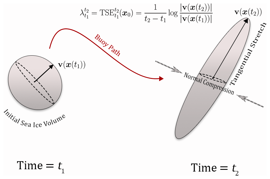
Figure 2 Example evolution of a small volume of sea ice surrounding a buoy in a steady flow. From time t₁ to t₂, the buoy velocity vector v(t)=v(x(t)) increases, leading to compression in the plane of sea ice orthogonal to the buoy trajectory and positive TSEs.

For real discrete observational trajectory data with an initial position x₀=x(0), we approximate the integrals in Eqs. (6) and (7) and define the trajectory-stretching exponents (TSEs) used for the remainder of this research:

$$\begin{array}{}\text{(8)}& {\displaystyle }{\mathrm{TSE}}_{t_{\mathrm{0}}}^{t_N}\left({\mathit{x}}_{\mathrm{0}}\right)={\displaystyle \frac{\mathrm{1}}{t_N-t_{\mathrm{0}}}}\log {\displaystyle \frac{\left|\dot{\mathit{x}}\right(t_N\left)\right|}{\left|\dot{\mathit{x}}\right(t_{\mathrm{0}}\left)\right|}}\text{(9)}& {\displaystyle }{\stackrel{\mathrm{‾}}{\mathrm{TSE}}}_{t_{\mathrm{0}}}^{t_N}\left({\mathit{x}}_{\mathrm{0}}\right)={\displaystyle \frac{\mathrm{1}}{t_N-t_{\mathrm{0}}}}\sum _{i=\mathrm{0}}^{N-\mathrm{1}}\left|\log {\displaystyle \frac{\left|\dot{\mathit{x}}\left(t_{i+\mathrm{1}}\right)\right|}{\left|\dot{\mathit{x}}\left(t_i\right)\right|}}\right|.\end{array}$$

As with λ, the TSE is positive for stretching and negative for compression along a trajectory. $\stackrel{\mathrm{‾}}{\mathrm{TSE}}$ does not allow for this cancellation as the summand is strictly positive and gives a measure of cumulative changes but does not differentiate stretching or compression, as with $\stackrel{\mathrm{‾}}{\mathit{\lambda }}$. The TSE and $\stackrel{\mathrm{‾}}{\mathrm{TSE}}$ have been shown to accurately separate dynamically distinct regions (eddies and fronts) in sparsely sampled open-ocean flows (Haller et al., 2021) but have not yet been studied in a sea ice context.

In contrast to Eqs. (2)–(3), TSEs do not differentiate between contributions from divergence or shear to the stretching of a material. Rather, they quantify stretching in the direction of vectors tangent to the buoy trajectory. We discuss the mathematical relationship between Eqs. (2)–(3), the closely related Lagrangian-averaged divergence (Szanyi et al., 2016a), and TSEs in Appendix A1. TSEs are calculated using only buoy speed and do not require projection to orthogonal velocity components as in Green's theorem approximations from arrays. Speed can be easily calculated using geodesics between GPS locations, which prevents any inconsistencies of results due to map projections. Furthermore, TSEs are parameter-free, with integration time being the only user-chosen value. The choice of integration time defines the average stretching extent but does not prevent identification of events at timescales shorter or longer than that. See Sect. 4.1 for one such example of hourly timescale events being identified by a multi-day integration window.

The sampling period may influence the estimated speed of each buoy (Lei et al., 2021) and should be mentioned when performing analysis with TSEs. Once raw data have been collected, the user may then resample the data at a higher or lower resolution. Changing this sampling period is akin to changing the resolution of a Riemann sum that is approximating an integral. That is precisely what Eqs. (8) and (9) are with respect to Eqs. (6) and (7). The choice of interpolation method would have analogous effects.

While Eulerian-strain-based metrics (Eqs. 1–3) provide an imperfect comparison to an approach to ice deformation that is based on a Lagrangian coherent structure, they are commonly used in sea ice dynamics research and generate long time series when polygons are suitably chosen (e.g., Hutchings et al., 2012; Itkin et al., 2017). TSEs are Lagrangian diagnostics and are calculated over a forward-looking window from a starting time, t₀ (Eqs. 8 and 9). By incrementally increasing t₀, we can also generate time series of TSE and $\stackrel{\mathrm{‾}}{\mathrm{TSE}}$ for each step in a buoy trajectory. In this way, large TSE and $\stackrel{\mathrm{‾}}{\mathrm{TSE}}$ time series values should slightly precede significant storms, sea ice stretching, or breakup events as the summation occurs from t₀ forward in time. This also means that TSE and $\stackrel{\mathrm{‾}}{\mathrm{TSE}}$ series will be slightly out of phase with concurrent Eulerian-polygon-based divergence, shear, and deformation series. Indeed, we find this phase difference is on the order of the length of the integration window when maximizing the cross-correlation between TSEs and div and D (Eqs. 1 and 3, not pictured). We refer the reader to Appendix A1 for a thorough numerical comparison of Eulerian and Lagrangian diagnostics in a simple geophysical model.

Results here focus on the ability of TSEs to accurately characterize spatially and temporally localized coherent stretching during short-lived midwinter storms. This choice is motivated by the availability of recent high-resolution experiments and local deformation being an open problem in sea ice dynamics (Oikkonen et al., 2017). As with other Lagrangian methods, the integration time is user-defined and reflects the duration over which we are seeking significant and coherent stretching. For example, previous LCS analysis using 6-month FTLE fields identified three distinct dynamic regions at pan-Arctic scales: the Fram Strait, Beaufort Gyre, and Northwind Ridge (Szanyi et al., 2016b). Similarly, TSEs are applicable to both short or long integration times (t_N−t₀) and reveal time-averaged dynamics at those specified scales. We refer the reader to Appendix A1 for a comparison of TSEs when varying integration times.

The choice of TSE integration window is only limited by the accuracy of the GPS trajectory data. Shorter integration times are likely affected more significantly by small discrepancies in GPS locations. The instantaneous limit of the TSEs is also well defined and provides approximations of hyperbolic (or parabolic) objective Eulerian coherent structures, which are the instantaneous limits of hyperbolic (or parabolic) LCSs (Serra and Haller, 2016; Nolan et al., 2020).

3 Datasets

Our results verify that TSEs can identify significant ice dynamics events using three different data sources at different spatial scales: synoptic storm analysis from a targeted experiment, linear kinematic feature (LKF) formation in subsequent SAR frames on the order of tens of kilometers, and sea ice brightness temperature measurements that show landfast and free-ice fractures at scales of hundreds of kilometers. We exhibit the utility of TSE and $\stackrel{\mathrm{‾}}{\mathrm{TSE}}$ spatiotemporal analysis for two experimental sea ice buoy datasets, the N-ICE2015 (Itkin et al., 2015, 2017) and MOSAiC expeditions (Krumpen et al., 2020), and data from the International Arctic Buoy Program (IABP) (International Arctic Buoy Programme, 2022).

3.1 N-ICE2015

The 6-month Norwegian young sea ice cruise (N-ICE2015) sought to understand the rapid shift to younger and thinner sea ice and its effect on energy fluxes, sea ice dynamics, and ecosystems in the Arctic basin. Numerous in-depth studies have evaluated the thin ice and weather conditions during the N-ICE2015 experiment (e.g., Cohen et al., 2017; Granskog et al., 2017; Itkin et al., 2017; Graham et al., 2019a). Itkin et al. (2017) conducted a thorough investigation of the ice response to N-ICE2015 storms, as identified by Cohen et al. (2017), which provides a test bed of buoy data where atmosphere–ice relationships during brief synoptic events are well understood (i.e., Itkin et al., 2015).

The experiment involved atmospheric, biogeochemical, oceanographic, and sea ice dynamics components, including two separate buoy deployments from January to mid-March and late April to June 2015 (Fig. 3). For our analysis, we focus on 24 buoy trajectories (Fig. 3) in two time windows previously examined by Itkin et al. (2017). GPS positions were primarily sampled at 1 h intervals, though some were sampled every 3 h. Itkin et al. (2017) resampled all trajectories to a 1 h⁻¹ sampling frequency using a linear interpolant, and we follow this convention for our N-ICE2015 analysis. After interpolation, subsequent buoy speeds that exceeded 5 km d⁻¹ were removed, and buoy positions were resampled using a linear interpolant.

Itkin et al. (2017) calculated divergence, shear, and deformation using a tessellation of buoy triads, removing some of the user dependence but potentially introducing triads with inappropriate geometry for the contour integral approach. In particular, the winter deployment of buoys for the N-ICE2015 campaign was hindered by logistical challenges as the researchers deployed buoys in the polar night by snow machines and on skis. This resulted in an initially quasi-linear buoy array geometry, with many of the triangles formed by buoy vertices having small angles (<15^∘). Upon removing the most unreliable calculations, Itkin et al. (2017) successfully showed the impact of the Cohen et al. (2017) storms on shear, divergence, and deformation signatures during the winter and spring deployments.

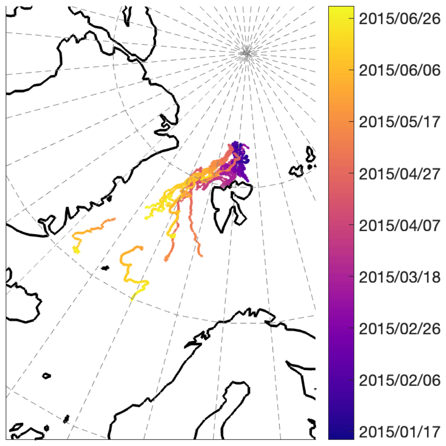
Figure 3 Trajectories of the N-ICE2015 buoys deployed north of Svalbard from January to June 2015, with positions colored by date.

3.2 MOSAiC

The Multidisciplinary drifting Observatory for the Study of Arctic Climate (MOSAiC) is the largest multidisciplinary Arctic expedition to date, spanning the winter of 2019–2020 (Krumpen et al., 2020). The study centered around the research icebreaker Polarstern (Knust, 2017; Nicolaus et al., 2022; Rabe et al., 2022) which was moored to an ice floe for an entire year. MOSAiC provides an unprecedented look at winter ice dynamics with 213 unique buoy deployments and complementary atmosphere, ocean, ecology, and biogeochemistry data.

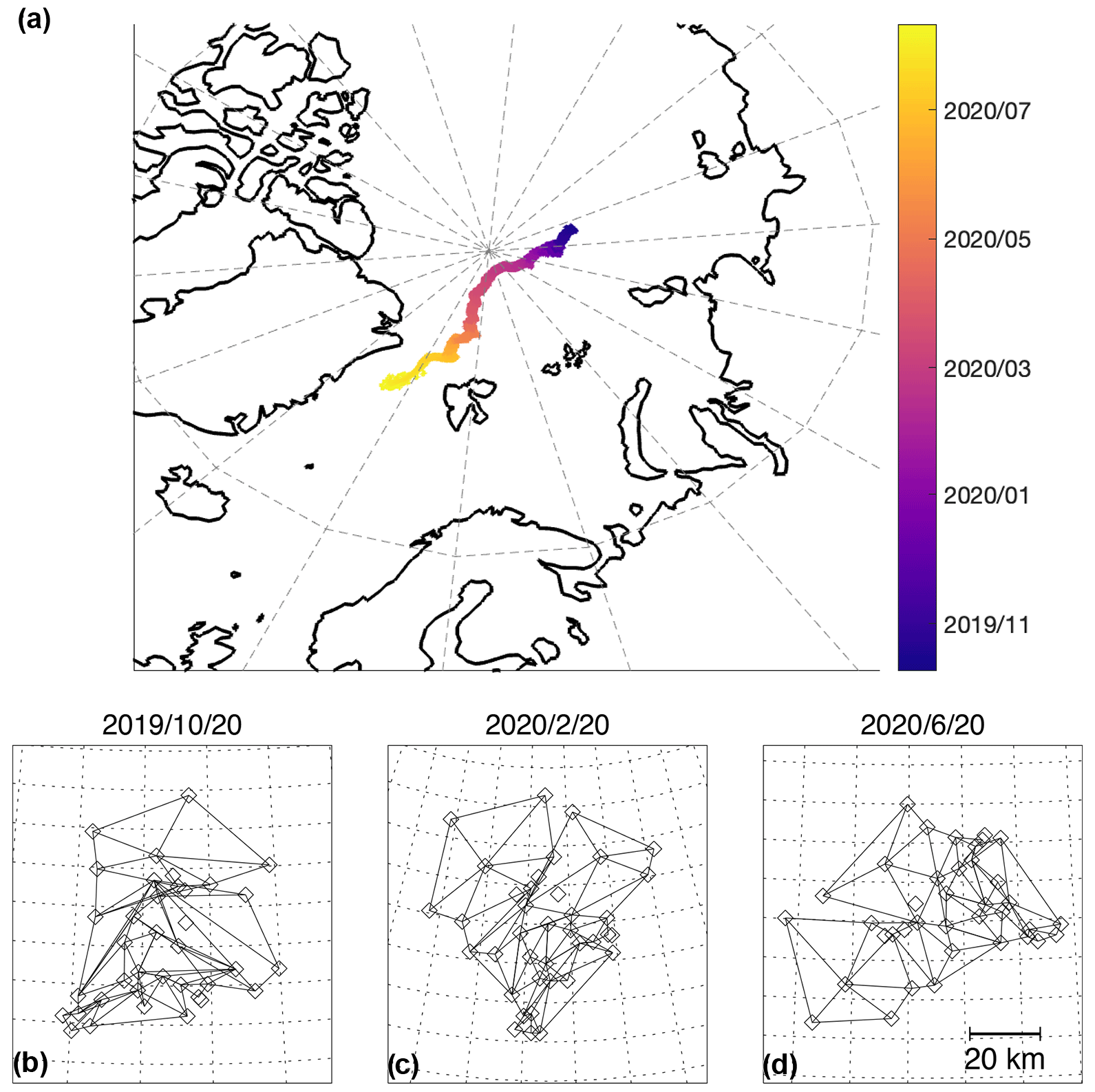
Figure 4 (a) Trajectories of the MOSAiC buoys from October 2019 to July 2020, with positions colored by date. (b–d) The MOSAiC buoys (diamonds) and triads (outlined with solid lines) as arranged for deformation calculation. The same array at three times is shown, with maps centered on (85.08^∘ N, 132.9^∘ E), (88.4^∘ N, 65.9^∘ E), and (81.9^∘ N, 8.3^∘ E) from (b) to (d) respectively. The scale of the maps is shown in the bottom right.

We focus here on the paths of 101 buoys deployed within 40 km of the Polarstern. This public dataset was documented by Bliss et al. (2023). The half-hourly buoy track data were cleaned following Hutchings et al. (2012). Triads were also handpicked from the MOSAiC buoys with data spanning October 2019 to June 2020, and this is the focus of a forthcoming publication. The arrays were selected to maintain reasonable shapes (no small angles, area greater than 1 km²) from the beginning to the end of the time series, and the public data were resampled to uniform 6-hourly intervals. Handpicking triads, however, does require user discretion. Buoy tracks were resampled to match the triad sampling rate. The arrays used are shown in Fig. 4. A deeper comparison and refinement of geometrically suitable arrays in the MOSAiC data is a current topic of research. The method we use here is in line with previous work (Hutchings et al., 2011, 2012).

Though MOSAiC analysis is now just beginning, there are currently limited midwinter buoy data available for the Arctic. MOSAiC and N-ICE2015 provide the best test beds for evaluating the efficacy of TSEs to identify significant stretching events at high spatial resolution in coherent ice floes.

3.3 IABP

The International Arctic Buoy Program (IABP; https://iabp.apl.uw.edu/data.html, last access: 3 March 2022) is a network of drifting buoys that have been deployed in the Arctic Ocean by a collection of nations since the 1970s. In comparison with the previous two experiments, IABP buoy density is significantly lower, but the length of the IABP buoy record and its considerable spatial coverage allows for analysis of ice dynamics at much greater scales (see Fig. 5). IABP data have been a useful ground truth of sea ice motion for several decades and continue to provide invaluable information for both model verification and understanding the complexities of ice dynamics (Rampal et al., 2009; Bouchat and Tremblay, 2020). IABP buoy tracks are available in both raw and cleaned formats. We focus our analysis on the publicly available 3-hourly L2 IABP buoy data. We downsampled the data with a 6 h sampling to maintain consistency with the MOSAiC data using a linear interpolant. We focus our analysis on trajectories during 2017 (Fig. 5), with particular interest in the well-studied Beaufort Sea.

Figure 5 Trajectories of the IABP buoys from 1 January 2017 to 1 January 2018.

4 Results

4.1 N-ICE2015

For our first evaluation of TSEs, we utilize previous storm analysis from the N-ICE2015 expedition. Cohen et al. (2017) studied winter storms during this sea ice cruise and found they typically occurred with a duration between 3 and 10 d. Using a buoy-array approach (Eqs. 1–4), Itkin et al. (2017) found that sea ice deformation events could be roughly coupled with the passage of these storms. As we wish to quantify coherent ice deformation over a given time window, we choose a 3 d integration period for stretching exponent calculations so as to capture the storm-scale Lagrangian stretching without averaging over too wide of a time window. In this way, TSE provides a before-and-after stretching measure, while $\stackrel{\mathrm{‾}}{\mathrm{TSE}}$ calculates the accumulation of trajectory stretching and contraction during the 3 d window.

Figure 6 details TSEs for the winter- and springtime windows analyzed by Itkin et al. (2017). The significant N-ICE2015 storms from Cohen et al. (2017) are shaded as pink regions and underlay plots of TSE and $\stackrel{\mathrm{‾}}{\mathrm{TSE}}$ for all buoys in the two deployments. In winter, every storm of note was preceded by local TSE extrema, including the short 10 h storm on 22 January and the 5 h storm on 13 February. These two storms are well below the timescale of TSE integration we have chosen (3 d) but are still evident in the TSEs. This is because TSEs look at average behavior over a given time, not specific events with a given duration.

Every coherent TSE peak above 1 d⁻¹ (marked by horizontal dashed line) was immediately followed by a significant storm in the TSE integration window, but local maxima do not always correspond to the passage of storms. This is likely due to oceanic influences not immediately related to the passage of storms. Itkin et al. (2017) calculated a significant divergence and shearing event for the buoy array on 26 January, which did not correspond with the presence of a storm but was instead related to a change in wind-direction. While the TSE and $\stackrel{\mathrm{‾}}{\mathrm{TSE}}$ are both sensitive to accelerations caused by changes in wind direction, values in Fig. 6a–b do not reveal such a coherent stretching event and indicate a possible advantage of using single-buoy stretching that is less reliant on buoy array geometry.

Storms during the spring deployment also coincided with significant stretching events, even for the sub-12 h storms on 16 May, 30 May, and 8 June. Similar to the analysis of Itkin et al. (2017), stretching time series for the spring deployment exhibited sub-daily oscillations, likely related to a more fractured sea ice cover, tides, or inertial motions. There is also a large variance in the underlying buoy velocities, which is potentially an effect of using a 1 h sampling window, where small variations can lead to large velocity fluctuations. Due to these fluctuations, we find $\stackrel{\mathrm{‾}}{\mathrm{TSE}}$ is less informative in spring as an increase in small fluctuations has a positive cumulative effect during summation and reveals less about the storm-scale dynamics.

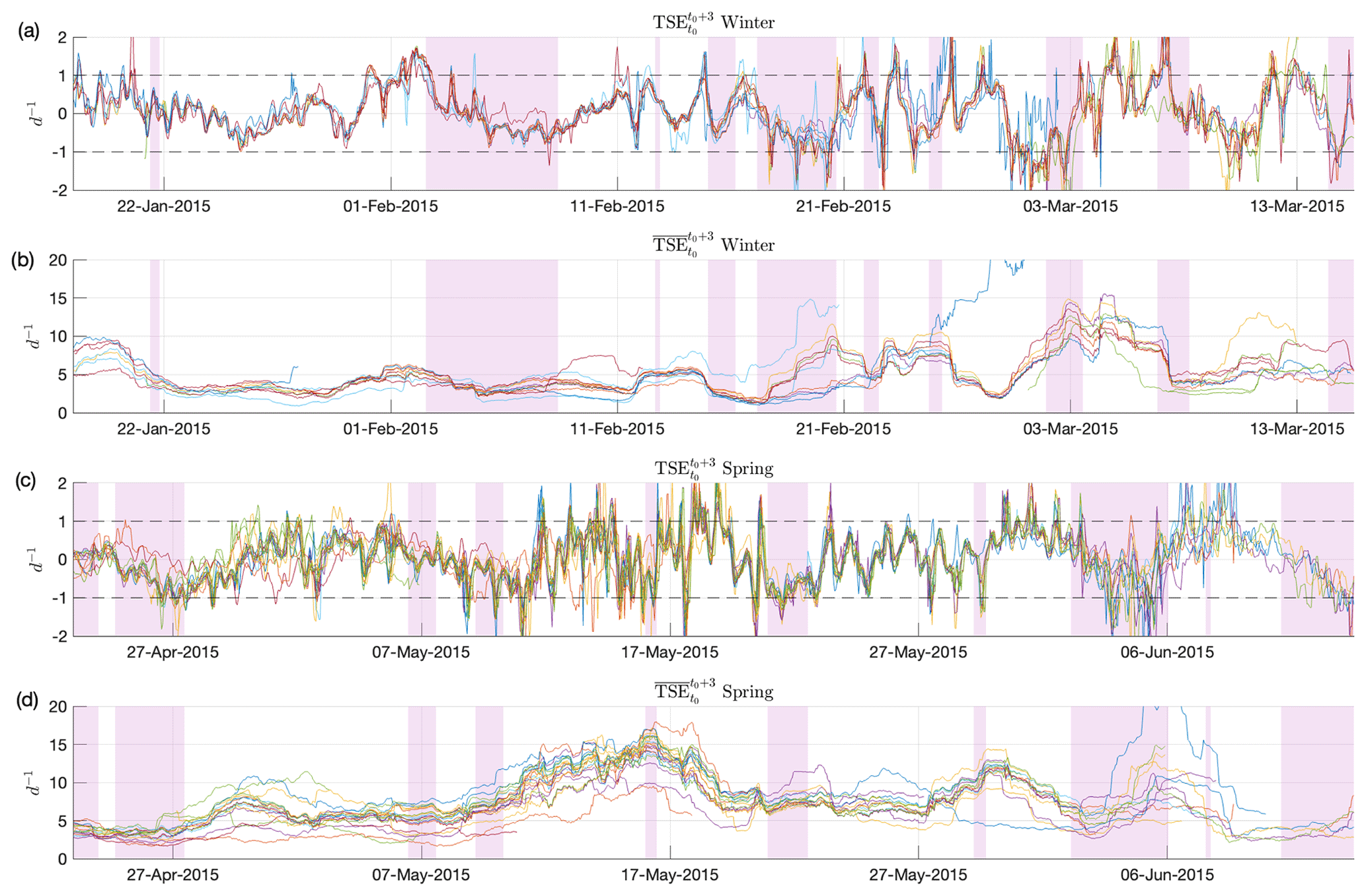
Figure 6 Comparison of TSE and $\stackrel{\mathrm{‾}}{\mathrm{TSE}}$ time series for 24 buoys during two stages of the N-ICE2015 experiment. Significant storm events for the winter deployment (a, b) and spring deployment (c, d) are shown as pink regions. A good correlation between strong stretching events and Arctic storms is shown: TSE extrema (>1 d⁻¹, marked by dashed lines) precede all storms and show no false positive sea ice stretching indicators.

4.2 MOSAiC

Our second example utilizes MOSAiC buoy data from November 2019 to April 2020. We again choose a 3 d integration window in the absence of an alternative integration scale. Should an exhaustive storm study, such as that conducted for N-ICE2015, be performed, revisiting this analysis may be insightful. While the effect of integration scale does have some effect on TSEs, identification of the underlying dynamical features is surprisingly robust (Appendix A1). In Fig. 7a–d we compare time series of TSEs (Fig. 7a) and $\stackrel{\mathrm{‾}}{\mathrm{TSE}}$ (Fig. 7c) with triad-based instantaneous approximations of divergence and deformation (Eqs. 1–4). We plot all TSE time series available (101) and again find there is impressive coherence in stretching exhibited by the entire cluster. Local values of TSEs and $\stackrel{\mathrm{‾}}{\mathrm{TSE}}$ also have the largest variance during peak stretching events. This allows us to both analyze the temporal localization of sea ice fracture by TSEs and potentially relate spatial differences of trajectory stretching to nearby LKFs. In Fig. 7b and d, blue dots indicate the instantaneous value from each buoy triad, and the black lines show the mean over all triangles.

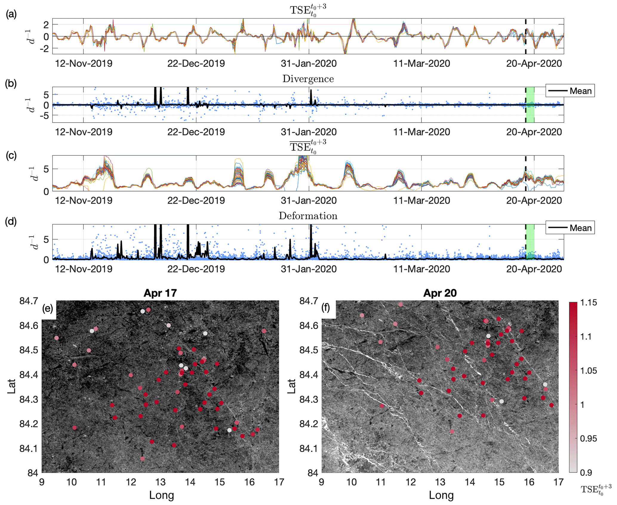
Figure 7 (a–d) Time series comparison of trajectory-stretching exponents and common buoy-array-based approximations of divergence of and total deformation during the MOSAiC expedition. The vertical dashed black lines show a sea ice fracture event that was largely missed in the divergence and deformation. Panels (e) and (f) show a before-and-after comparison of HH Sentinel-1 frames surrounding the 17 April spike. Over this time span, the creation of multiple LKFs in white can be seen, as well as the concurrent TSE values of nearby buoys.

Qualitatively, prior to the 31 January event there is a reasonable agreement between TSEs and triad-based events, when accounting for the 3 d integration window. For the entire period, one finds that all strong divergence and deformation events are accounted for as extrema (>1 d⁻¹) in the TSEs, though often with a different relative magnitude. In mid-November 2019, large TSE magnitudes generate a spike in $\stackrel{\mathrm{‾}}{\mathrm{TSE}}$ that is also evident as spikes in div and D. Local $\stackrel{\mathrm{‾}}{\mathrm{TSE}}$ maxima in middle and late December also correlate well with spikes in div and D. Mean div provides a suggestion of whether divergence or convergence was more prevalent amongst the triads at a given time, but the significant scatter of both positive and negative values obscures such behavior at finer spatial scales. In contrast, there is much less ambiguity of the characteristic ice behavior for the entire cluster in the TSE series, suggesting the cluster remained part of a largely coherent structure that stretched and compressed together, with variance between buoys appearing during dynamic events.

After 31 January, several relatively large peaks in TSEs appear as minor oscillations in div or D or are not present. This indicates local dynamic stretching and potential fracture events may not be evident with the contour integral metrics. One such example is shown for the peak on 17 April, highlighted by the vertical dashed black line. In div and D plots, we also show the 3 d integration window in green. This example was chosen due to the concurrent availability of pre- and post-storm SAR data during the period after the major 31 January event, as well as a relatively minor signature in div and D. The large stretching indicated by TSEs on 17 April corresponds with multiple leads that formed throughout the domain of the MOSAiC buoys. These fractures can be seen in the pair of HH polarization Sentinel-1 frames (Copernicus, 2020) (Fig. 7e–f), where white regions indicate new ice forming in leads or wind-driven waves (Grenfell et al., 1998). Points showing buoy locations have been colored by the 17 April TSE values. The spatial distribution of TSE values is difficult to interpret and would require a deeper analysis of the meteorological and ice conditions.

In the 3 d window following the 17 April TSE and $\stackrel{\mathrm{‾}}{\mathrm{TSE}}$ peak, the mean buoy divergence oscillated around zero (Fig. 7b), with the magnitude staying below 0.1 d⁻¹. This is approximately 1 % of peak values of mean divergence, suggesting a relatively insignificant period of divergence. This is in contrast to the TSE and $\stackrel{\mathrm{‾}}{\mathrm{TSE}}$ on 17 April, which sits at approximately 50 % of their total peak values, suggesting a relatively localized motion with a larger contribution to ice dynamics at the same time.

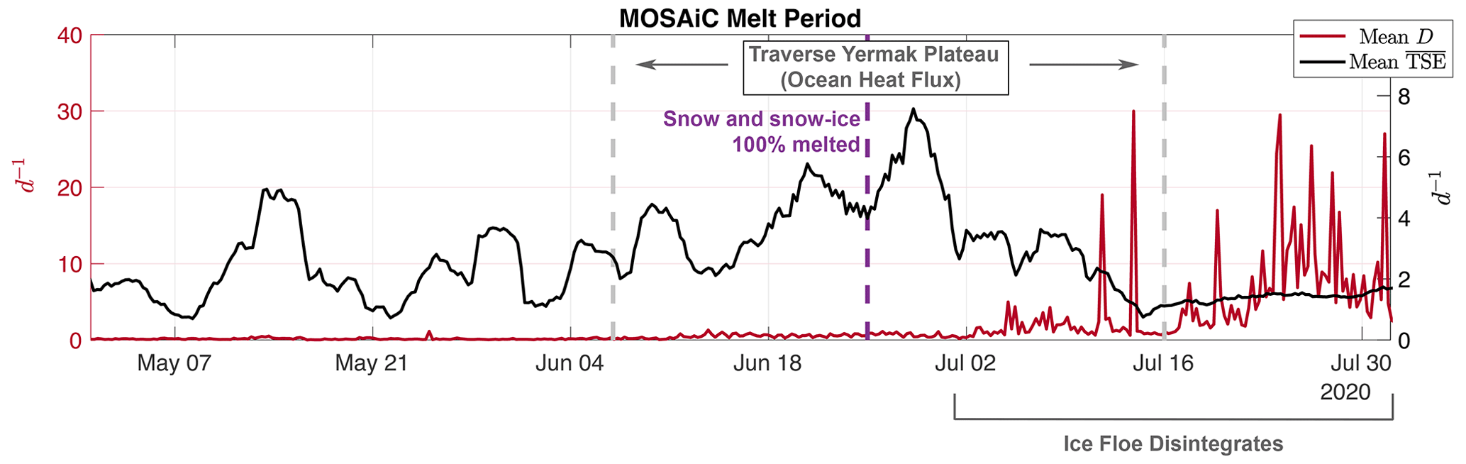
Figure 8 Average TSE and D during the MOSAiC melt period. A gradual increase in trajectory stretching is found until the onset of ice floe disintegration. Peak stretching was found immediately after all snow and snow ice was melted off the ice floe. Much larger $\stackrel{\mathrm{‾}}{\mathrm{TSE}}$ variance was found after a period of enhanced ocean heat flux as the ice floe crossed the Yermak Plateau. At this stage, the ice concentration dropped below 60 %–85 %, mean $\stackrel{\mathrm{‾}}{\mathrm{TSE}}$ values look flat from uncorrelated motions, and mean D spikes are an order of magnitude larger than when the ice floe remained intact.

The contribution to total deformation from shear was slightly larger, with a peak mean deformation of 0.46 d⁻¹ at 17:00 UTC on 17 April. The choice of triangles dictates which LKFs are spanned during this dynamic event and may explain why there was a weak deformation signature from the triads. As well, the lack of objectivity or trapezoid rule errors when using Green's theorem approximations with triads, as detailed in Appendix A2, may also contribute. In this scenario, the stretching and relaxation measured by the TSE present a clear correlation with material deformation of the ice and suggest TSEs may provide ice behavior insight during times when Green's theorem methods are not possible, such as when there are too few buoys or they are their orientation is inappropriate and when array-based approaches have underestimated dynamic behavior.

As sea ice melts in spring, ice concentration drops, and the ice pack loses integrity, TSEs and rate-of-strain diagnostics are no longer strictly representing the deformation of the ice cover. In Fig. 8, we look at mean $\stackrel{\mathrm{‾}}{\mathrm{TSE}}$ and mean D during different stages of the melt period identified by Lei et al. (2022). In late spring, $\stackrel{\mathrm{‾}}{\mathrm{TSE}}$ values increase as the ice becomes more dynamic. Once the ice floe enters warmer upper-ocean water over the Yermak Plateau, basal melting increases, and $\stackrel{\mathrm{‾}}{\mathrm{TSE}}$ oscillations trend upwards. At the same time, oscillations in D also begin to increase. By 25 June, snow and snow ice had completely melted from the sea ice cover, further enhancing the surface melt rates. After this, we obtain peak $\stackrel{\mathrm{‾}}{\mathrm{TSE}}$ values for the year, followed by a sharp drop. It is at the end of this sharp decline in stretching that Krumpen et al. (2021) note the ice floe begins to disintegrate. We hypothesize that $\stackrel{\mathrm{‾}}{\mathrm{TSE}}$ spikes precisely because this onset of disintegration enters the integration window.

At the timing of this drop in $\stackrel{\mathrm{‾}}{\mathrm{TSE}}$ and onset in disintegration, D values also obtain large values never seen before in the flow. The sea ice concentration now drops to between 60 % and 85 %, depending on location of the buoy. From here on, buoy trajectories are no longer correlated, and each buoy's $\stackrel{\mathrm{‾}}{\mathrm{TSE}}$ is measuring different dynamical flow features. At this stage, a mean $\stackrel{\mathrm{‾}}{\mathrm{TSE}}$ is no longer meaningful. However, future research may investigate spatially resolving single-trajectory flow features for heavily fractured ice floes, as has been done with analogous techniques in the open ocean (Encinas-Bartos et al., 2022).

4.3 IABP

In this section, we focus specifically on behavior in the Beaufort Sea from October 2016 to October 2017. During this winter, thinner-than-usual sea ice may have caused the collapse of a typical high-pressure system over the Beaufort and anomalous surface winds (Moore et al., 2018). We again choose a 3 d integration window for our study to maintain comparability with the previous examples, though other timescales are equally applicable.

In Fig. 9a, we show the 3 d TSE for each buoy in the Beaufort during that period in gray. The maximum distance between buoys sampled here is approximately 30 times the length scale of the previous experiments. Due to the sparse sampling over a much larger spatial domain, there is much more variance around the mean TSE value, shown in black in Fig. 9a. The absolute maximum of mean TSEs during this period is indicated by a red dot, signifying a period of maximal stretching and deformation over a large domain. The following two peaks are also identified by red dots. These events correspond with three dynamic shifts in Beaufort Sea ice structure and behavior. The frame pairs in Fig. 9b–d show before-and-after frames of AMSR2 Sea Ice Brightness Temperature (89 V GHz) (Meier et al., 2018) for times corresponding to high TSE values. Buoy positions are again colored by TSEs in the initial frame, and color maps are consistent across all frames. Please review the “Video supplement” section for further information and a full animation of this breakup event.

The first event corresponds to stretching from 26 to 29 March 2017. Previous mean TSE oscillations gradually increased to the absolute maximum of mean TSEs on 26 March. Prior to any evidence of detachment of the mobile pack ice in the Beaufort Sea, TSE values were indicating an ongoing increase of stress and strain, leading to the major fracturing in March and April 2017.

Between 26 and 29 March, an initial significant fracture formed when the mobile Beaufort pack ice separates from the landfast ice on the northern coast of Alaska. The fracture extends to just off the coast of Banks Island (BI in Fig. 9c) as the ice in the Beaufort Gyre begins to freely rotate in an anticyclonic motion. All buoys in the free-drift region have large positive (red) TSE values and create another local maximum in the mean time series, further supporting this relatively significant stretching event in March and April when compared to times prior to and after these months. From 3 to 8 April, significant fracturing throughout the region south of 76^∘ N occurred, with another major fracture extending off the northwest corner of Banks Island. The buoys in the region of this enhanced fracturing showed large positive TSE values, whereas buoys further north without new fracturing showed low TSE values. The last pair of frames show the last major shift in ice dynamics from 13 to 17 April. At this time, a major lead formed off Prince Patrick Island (PI). This was the last stage of the changing dynamics, after which all ice south of the PI lead exhibited a much freer anticyclonic rotation, decoupled with the surrounding ice. Again, the largest positive TSE values were found in the spatial domain where significant ice breakup was occurring, with lower TSE values, hundreds of kilometers away, delimiting the fracture domain to the north. After the 17 April fracturing, TSE values remain relatively low compared to these distinct peaks, similar to the behavior of the MOSAiC buoys during the disintegration of the ice floe in Sect. 4.2.

One specific benefit displayed in this example is the significant spatial extent of the large positive TSE values prior to each fracture in the Beaufort Gyre. Not only was the edge of the gyre identified in the gap between positive and negative TSEs, but a positive TSE was also found 1000 km from the Prince Patrick and Banks Island fractures on the western edge of the gyre. This supports the ability of TSEs to identify the Lagrangian coherent structures in the mobile pack ice as a whole, not just locally highlight a fracture.

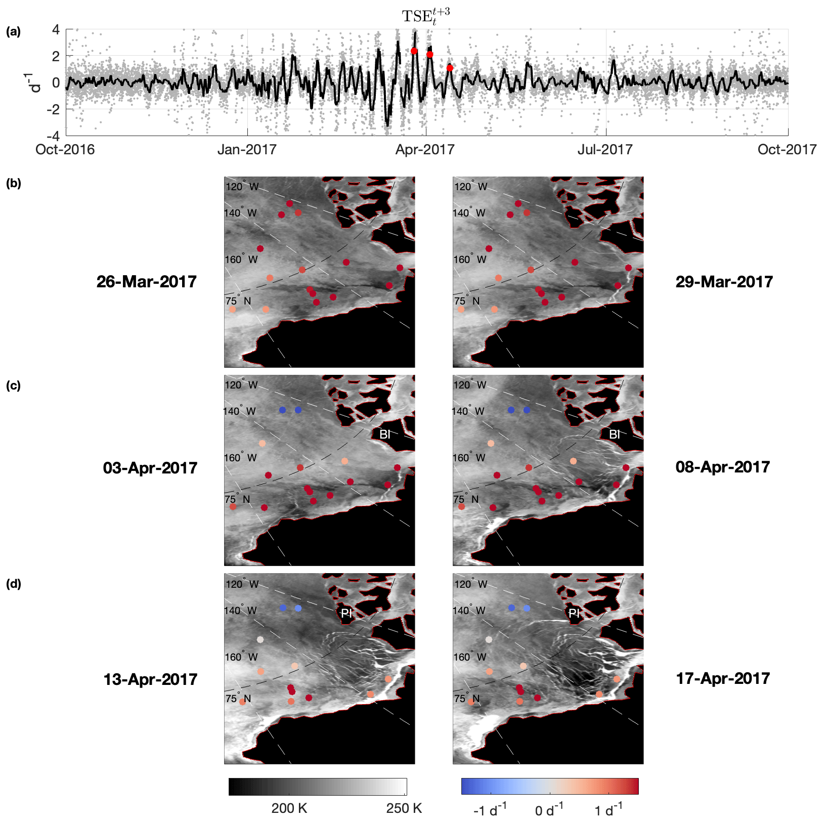
Figure 9 (a) Time series of TSEs for buoys in the Beaufort Sea from October 2016–2017, with mean shown in black. Red points correspond to local maxima of TSEs as the ice breaks into a state of free drift. (b–d) The three steps of the Beaufort Gyre sea ice freeing itself from surrounding ice beginning its spring anticyclonic acceleration, corresponding with the three highlighted TSE spikes in (a). Before and after brightness temperature images show the significant fractures at the northern coast of Alaska (b), Banks Island (c), and Prince Patrick Island (d).

5 Conclusions

We find that TSEs successfully identify significant local material deformation tangent to individual sea ice buoy trajectories. Periods of strong local stretching are representative of changing ice dynamics in a neighborhood to 10–1000 km. That is, though TSEs are local in nature, their values provide insight into much larger coherent sea ice structures and distant fracture events. This local–regional connection provides a valuable avenue for researching sea ice dynamics in sparsely sampled regions and understanding the changing rheology of sea ice. In contrast, conventional polygon-based approaches provide an estimate of the spatial average of divergence, shear, or deformation over an ice volume, with errors increasing as the area decreases, the number of buoys decreases, or the array becomes skewed.

Approaching sea ice dynamics through quasi-objective stretching, we were able to capture coherent deformation events in concentrated and sparsely sampled buoy experiments. Spatial and temporal signatures of stretching with TSEs are well correlated with formation of nearby leads and changing ice transport patterns, as well as with the concurrence of well studied sea-ice-impacting storms. For two high-resolution midwinter buoy deployments, we find that the TSEs had greater sensitivity to sea ice deformation than the common polygonal approach and potentially avoided a false positive identification.

Specifically, large TSE values coincided with major storms in the N-ICE2015 experiment and did not identify a mysterious storm-free dynamic ice event that was described by Itkin et al. (2017). For the first half of the MOSAiC experiment, we found a good qualitative agreement between polygon-based metrics and the TSEs, though this correlation was much weaker following a large midwinter storm. During this latter half, we verified TSEs were able to identify an influential stretching event that was much less evident with Green's theorem methods. Lastly, TSEs were able to spatially and temporally isolate major fracture events during Beaufort Sea ice breakup using IABP data at a much lower spatial resolution. A buildup of stress in the Beaufort Sea was detailed by increasing local TSE maxima, until an initial separation formed at the land-fast ice during the seasonal TSE peak. During subsequent diminishing peaks, the ice fractured and further detached from land-fast regions, creating a coherent mass of rotating ice that was delimited spatially with TSEs. TSE events with increasing amplitude preceded spring breakup events in both high-resolution MOSAiC and sparsely sampled IABP data. This suggests the predictive abilities of TSEs may possibly be developed with further investigation.

The single-buoy quasi-objective trajectory-stretching exponents (TSEs) identify dynamic sea ice events that are potentially significant in terms of understanding spatially and temporally varying sea ice deformation. As sea ice dynamics plays an important role in atmosphere–ice–ocean exchange processes, we find the further event-detection sensitivities possible with TSEs are a valuable complement to common, polygon-based divergence, shear, and deformation approximations. We find TSE usage provides some distinct advantages and potential improvements for future research:

1. TSEs identify deformation events from a single buoy and are thus unaffected by buoy array geometry or the number of buoys deployed. As buoys passively follow ice floes, we can still obtain insights into ice dynamics as arrays become heavily skewed and non-uniform. The TSE maintains integrity in this situation, whereas arrays of buoys become aligned and unsuitable for strain estimates due to shearing in the ice pack. This expands the domain of potential analysis and reduces logistical burdens of Arctic and Antarctic expeditions as stretching dynamics can be studied with TSEs from linear, randomly distributed, or organized arrays. This is particularly valuable for the Antarctic, where there are significantly fewer buoys deployed than in the Arctic.

2. As TSEs are quasi-objective metrics in continua, their values provide a useful proxy for frame-indifferent (objective) measures of stretching, with a quantitative difference depending on the compressibility of the ice and slowly varying nature of the flow. In a heavily fractured ice context, the degree to which these single-trajectory metrics approximates along-trajectory ice stretching varies, but this work suggests positive correlations with remotely sensed dynamic fracture and breakup events. Further numerical and observational experiments can help improve these correlations.

3. TSE values do not need to be separated or averaged based on length scales (e.g., Itkin et al., 2017) and showed great success in identifying fracture regions at a wide range of spatial scales.

4. TSE calculations are mathematically simple as the TSE is calculated using only buoy speed and does not require projection to orthogonal velocity components. Speed can be calculated using geodesics between GPS locations, which prevents any inconsistencies of results due to choice of map projection or projection distortions, or needing to perform differential calculus in an elliptic geometry. Furthermore, the TSE is parameter-free, with integration time being the only user-chosen value.

Calculating TSEs from single buoy trajectories requires significantly less effort than SAR-based approaches, is not subject to the same errors (e.g., Bouchat and Tremblay, 2020), and also supplements data in the pole hole during winter (e.g., Krumpen et al., 2021). If we can further verify the slowly varying nature of sea ice at sub-diurnal timescales, TSEs may also fill in temporal gaps due to the sparse monitoring of satellites. Calculating TSE fields from more general feature trajectories, such as from X-band and high-frequency (HF) radar or SAR datasets, would be a straightforward application of Eqs. (8) and (9) and can also enrich the analysis of sea ice dynamics in existing datasets.

The ability of TSEs to overcome some of the shortcomings of other buoy approaches may also provide an additional source of deformation information, such as is necessary to constrain and improve sea ice models (Bouchat and Tremblay, 2020). To obtain rate-of-strain invariants for sea ice deformation, it is still necessary to use a high-density buoy array. Such an array also reveals gradients of trajectory stretching and further enhances precise stretching localization with TSEs. A modeling study of compressibility, slowly varying impacts, and sampling frequency would be useful for TSE applications in model development, as would a further comparison with divergence, deformation, and shear to aid the broader community in the physical interpretation of TSE signals. This would help interpret TSEs as complementary sources of stretching information when buoy arrays are aligned linearly due to strong shear, have edges that span large distances encompassing multiple fractures or coherent structures, or have areas below tolerable error thresholds. In remote polar regions where data are still difficult to obtain, but the changing climate has an outsized impact, TSEs provide new physics-based insights into ice dynamics while only requiring single GPS tracks.

Our findings suggest that spatiotemporal analysis of local and regional sea ice dynamics should be revisited with a comparison between single-trajectory and spatial velocity gradients. Our comparisons suggest potentially significant dynamic events in terms of understanding atmosphere–ice–ocean exchange processes may go undetected using conventional polygon-based methods or, in the case of N-ICE data, may be inaccurately detected. This advantage stems from the TSEs' ability to identify stretching in a small neighborhood of individual buoys and connect local changes with broader ice behavior. A deeper understanding of TSEs connection to more broadly used ice dynamics metrics will help researchers understand how TSEs can inform ice responses to various forcings.

Appendix A: Introduction

The first section of the Appendix develops the rigorous connection of trajectory-stretching exponents to more common deformation diagnostics through the rate-of-strain tensor and Cauchy–Green strain tensor. The second section of the Appendix provides a simple analytic example of buoy motion to illuminate Green's theorem estimation errors for a buoy-array diagnostic. This example shows how Green's theorem approximation fails to provide self-consistent divergence quantification (in a divergence-free flow), depending on equilateral triad orientation. The last section of the Appendix provides an assessment of the assumption that sea ice is a slowly varying flow to satisfy criteria for the quasi-objectivity of TSEs.

A1 Relating TSEs to shear and divergence

A1.1 Background

From the gradient of a two-dimensional velocity field v(x,t),

$$\mathrm{\nabla }\mathit{v}=\left(\begin{array}{cc}\frac{\partial u}{\partial x}& \frac{\partial u}{\partial y}\\ \frac{\partial v}{\partial x}& \frac{\partial v}{\partial y}\end{array}\right),$$

we can define the rate-of-strain tensor

$$\begin{array}{}\text{(A1)}& \mathbf{S}(\mathit{x},t)={\displaystyle \frac{\mathrm{1}}{\mathrm{2}}}(\mathrm{\nabla }\mathit{v}+\mathrm{\nabla }{\mathit{v}}^T).\end{array}$$

We can express the common Eulerian sea ice deformation metrics, divergence, and shear, as functions of the eigenvalues (principal stresses) of Eq. A1:

$$\begin{array}{}\text{(A2)}& {\displaystyle }\mathrm{div}=\mathrm{tr}\left(\mathbf{S}\right)={\mathit{\lambda }}_{\mathrm{1}}+{\mathit{\lambda }}_{\mathrm{2}}\text{(A3)}& {\displaystyle }\mathrm{shr}=\sqrt{\mathrm{tr}(\mathbf{S}{)}^{\mathrm{2}}-\mathrm{4}\det (\mathbf{S})}=\sqrt{({\mathit{\lambda }}_{\mathrm{1}}-{\mathit{\lambda }}_{\mathrm{2}}{)}^{\mathrm{2}}-\mathrm{2}{\mathit{\lambda }}_{\mathrm{1}}{\mathit{\lambda }}_{\mathrm{2}}}\text{(A4)}& {\displaystyle }D=\sqrt{{\mathrm{shr}}^{\mathrm{2}}+{\mathrm{div}}^{\mathrm{2}}}.\end{array}$$

To quantify the deformation of a material over time, one considers the flow map

$$\begin{array}{}\text{(A5)}& F_{t_{\mathrm{0}}}^t\left({\mathit{x}}_{\mathrm{0}}\right)=\mathit{x}(t;t_{\mathrm{0}},{\mathit{x}}_{\mathrm{0}})\end{array}$$

that takes an initial position x₀ to its current position $\mathit{x}(t;t_{\mathrm{0}},{\mathit{x}}_{\mathrm{0}})$ following the trajectory defined by the different equation

$$\dot{\mathit{x}}=\mathit{v}(\mathit{x},t).$$

From the gradient of the flow map, we define the right Cauchy–Green strain tensor as

$$\begin{array}{}\text{(A6)}& \mathbf{C}\left({\mathit{x}}_{\mathrm{0}}\right)=\left[\mathrm{\nabla }{F}_{t_{\mathrm{0}}}^t\right({\mathit{x}}_{\mathrm{0}}\left){]}^T\mathrm{\nabla }{F}_{t_{\mathrm{0}}}^t\right({\mathit{x}}_{\mathrm{0}}).\end{array}$$

Invariants of C are commonly used to study the deformation of material in continuum mechanics (Truesdell and Noll, 2004). In an incompressible two-dimensional flow, the rate of length change for an infinitesimal material element vector l based at the point x is

$$\begin{array}{}\text{(A7)}& {\displaystyle \frac{\mathrm{1}}{\mathrm{2}}}{\displaystyle \frac{\mathrm{d}}{\mathrm{d}t}}|\mathit{l}{|}^{\mathrm{2}}=\langle \mathit{l},\mathbf{S}(\mathit{x},t)\mathit{l}\rangle .\end{array}$$

Likewise, consider a curve γ parameterized by the dummy-time variable s that is evolving under the flow map, $F_{t_{\mathrm{0}}}^t\left({\mathit{x}}_{\mathrm{0}}\right)$. This could represent the evolution of a line of dye in a fluid or a physical transect along sea ice. A vector ξ₀ tangent to γ at x₀ evolves as ${\mathit{\xi }}_t=\mathrm{\nabla }{F}_{t_{\mathrm{0}}}^t{\mathit{\xi }}_{\mathrm{0}}$. It then follows that

$$\begin{array}{}\text{(A8)}& |{\mathit{\xi }}_t{|}^{\mathrm{2}}=\langle \mathrm{\nabla }{F}_{t_{\mathrm{0}}}^t({\mathit{x}}_{\mathrm{0}}){\mathit{\xi }}_{\mathrm{0}},\mathrm{\nabla }{F}_{t_{\mathrm{0}}}^t({\mathit{x}}_{\mathrm{0}}){\mathit{\xi }}_{\mathrm{0}}\rangle =\langle {\mathit{\xi }}_{\mathrm{0}},{\mathbf{C}}_{t_{\mathrm{0}}}^t{\mathit{\xi }}_{\mathrm{0}}\rangle .\end{array}$$

In the case that l or ξ₀ are eigenvectors of their respective tensors, Eqs. (A7) and (A8) equal the respective eigenvalues λ_i, which represent the stretching of an infinitesimally small sphere into an ellipse along its principal axes (Haller, 2015). When ξ₀ is the eigenvector associated with the larger Cauchy–Green eigenvalue, λ₂, one easily obtains the widely used finite-time Lyapunov exponent,

$$\mathrm{FTLE}={\displaystyle \frac{\mathrm{1}}{t_{\mathrm{1}}-t_{\mathrm{0}}}}\log \left({\mathit{\lambda }}_{\mathrm{2}}\right(\mathbf{C}\left)\right).$$

Otherwise, one can define the averaged stretching exponent

$$\begin{array}{}\text{(A9)}& {\mathit{\lambda }}_{t_{\mathrm{0}}}^t={\displaystyle \frac{\mathrm{1}}{t-t_{\mathrm{0}}}}\log {\displaystyle \frac{\left|{\mathit{\xi }}_t\right|}{\left|{\mathit{\xi }}_{\mathrm{0}}\right|}},\end{array}$$

also known as the finite-time Lyapunov exponent associated with the initial vector ξ₀. Due to the exponential growth of fluid particle separation and chaotic nature of fluid flows, one often utilizes stretching exponents in this context instead of eigenvalues of deformation tensors, though they are clearly closely related.

Lagrangian-averaged versions of shear and divergence can also be computed as

$$\begin{array}{}\text{(A10)}& \begin{array}{rl}& {\mathrm{LS}}_{t_{\mathrm{0}}}^t={\displaystyle \frac{\mathrm{1}}{t-t_{\mathrm{0}}}}\underset{t_{\mathrm{0}}}{\overset{t}{\int }}\mathrm{shr}\left(\mathit{x}\right(s\left)\right)\mathrm{d}s,\\ & {\mathrm{LAD}}_{t_{\mathrm{0}}}^t={\displaystyle \frac{\mathrm{1}}{t-t_{\mathrm{0}}}}\underset{t_{\mathrm{0}}}{\overset{t}{\int }}\mathrm{div}\left(\mathit{x}\right(s\left)\right)\mathrm{d}s,\end{array}\end{array}$$

respectively. LAD was previously used by Szanyi et al. (2016a) to differentiate between different contributions to the FTLE at pan-Arctic scales.

To calculate the rate-of-strain tensor, once must calculate spatial derivatives of the velocity field. Similarly, the right Cauchy–Green strain tensor requires the spatially and temporally resolved velocity field information to accurately calculate the gradient of the flow map. These sorts of spatially and temporally resolved velocity data are unavailable from sparse buoy trajectories. TSEs are designed to complement deformation metrics in sparse data settings.

Consider a trajectory x(t). One can calculate the Lagrangian velocity vector along the trajectory

$$\mathit{v}\left(t\right)=\mathit{v}\left(\mathit{x}\right(t\left)\right)=\dot{\mathit{x}}\left(t\right),$$

but we do not have any information about nearby velocities. Haller et al. (2021) show that, in a reference frame where the velocity field is steady (does not change with time), x(t) is a material curve, and v(t) evolves as a tangent vector to the trajectory. Thus the stretching of v(t) is a measure of material stretching along the trajectory, and we can closely approximate the averaged stretching exponent in that frame without the need of spatial derivatives. That is, in a steady flow (no time dependence), the TSE measures the correct stretching of Lagrangian velocity vectors as they materially evolve in that reference frame, as determined by the gradient of the flow map.

The instantaneous limit of TSEs corresponds with the analogous Eulerian rate of length change (Eq. A7) for the choice of vector l=v(t₀). In the following examples we highlight the ability of TSEs and $\stackrel{\mathrm{‾}}{\mathrm{TSE}}$ to delineate distinct coherent flow features without the use of spatial derivatives and compare their behavior with other diagnostics. These models are idealized flows without many of the complication from sea ice motion. That is, they represent steady-flow incompressible flow fields of a continuous medium and are thus ideal for comparing these diagnostics.

A1.2 Examples

For our first example, we compare Eulerian and Lagrangian diagnostics for the widely studied model of geophysical fluid flow (see, e.g., Rypina et al., 2007), the steady Bickley flow. The stream function of the flow is given by

$$\begin{array}{}\text{(A11)}& \begin{array}{rl}\mathit{\psi }(x_{\mathrm{1}},x_{\mathrm{2}})& =c{x}_{\mathrm{2}}-U_{\mathrm{0}}L\tanh (x_{\mathrm{2}}/L)\\ & +A{U}_{\mathrm{0}}L{\mathrm{sech}}^{\mathrm{2}}(x_{\mathrm{2}}/L)\cos k{x}_{\mathrm{1}},\end{array}\end{array}$$

where we use the geophysically based parameters $U_{\mathrm{0}}=\mathrm{62.66}\times {\mathrm{10}}^{-\mathrm{6}}$, L=1.77, $c=U_{\mathrm{0}}/\mathrm{2}$, A=0.1, r₀=6.371, $k=\mathrm{6}/r_{\mathrm{0}}$. As the velocity field is derived from the stream function, the velocity field is divergence-free. The flow consists of a central westward jet, two eastward jets above and below, and clockwise vortices. Figure A1 shows streamlines and velocity vectors for this flow, as well as divergence, shear, and vorticity fields calculated on a 500 × 150 grid. Note that the div=0 by design and that the vortex cores align when comparing streamlines and vorticity contours. Shear (Fig. A1c) shows a shear-free core and high shear regions adjacent to the jet and vortices, though contours of shear do not agree with the topology suggested by the streamlines or vorticity. This indicates that shear is not a good indicator of the edges of all coherent structures.

Figure A2 details TSE and $\stackrel{\mathrm{‾}}{\mathrm{TSE}}$ fields for a 500 × 150 grid of initial conditions, calculated from a trajectory integration time of 90 d. We also calculate LS (see Eq. A10; Fig. A2c) for each trajectory x(s). For brevity we omit LAD as the flow is divergence-free.

Contours of TSEs or $\stackrel{\mathrm{‾}}{\mathrm{TSE}}$ organize particles with similar trajectory stretching and reveal coherent structures of the flow. Note that both TSE and $\stackrel{\mathrm{‾}}{\mathrm{TSE}}$ can identify the edges of the central jet and eddies as shown in the streamlines of this steady flow. $\stackrel{\mathrm{‾}}{\mathrm{TSE}}$ also reveals where cumulative trajectory-tangent stretching is greatest, near the edges of the eddies. TSE provides intricate stretching and compression information surrounding the vortex cores and hyperbolic saddles, suggesting a complex stretch–relax cycle for material in the flow. The LS also does a much better job than Eulerian shear to extract the boundaries of each feature and also highlights the stronger shear near the edges of the central jet.

These underlying structures and their subsequent influence on sea ice deformation is exactly the kind of information that TSEs provide for sea ice dynamics analysis. As can be seen, mathematically there is limited relationship between the Eulerian metrics (Eqs. A2–A4) and the stretching exponents (Eq. A9), particularly because ξ is not necessarily aligned with the eigenvectors of S. Qualitatively, one can see there is no relation between div and TSEs for this simple example and very limited similarity with shear, except when evaluating a Lagrangian average (LS).

We also examine the influence of integration time on TSEs for this steady flow. In Fig. A3, we increase the integration time of particle trajectories from 1 to 30 d and plot TSE and $\stackrel{\mathrm{‾}}{\mathrm{TSE}}$ contours. The eddies, saddles between eddies, and central jet are evident for all integration times, but the clarity of boundaries increases as integration time increases. Note this improvement is not always possible with time-dependent flows as features may change. In more complex turbulent flows, such clarity at higher integration times can also be hindered by trajectories traveling near multiple uncorrelated coherent structures.

For our second example we use, there is in fact no reliable relationship to be inferred between TSEs and shear with a simple divergent flow:

$$\begin{array}{}\text{(A12)}& {\displaystyle }{v}_{\mathrm{1}}=x_{\mathrm{1}}\text{(A13)}& {\displaystyle }{v}_{\mathrm{2}}=x_{\mathrm{2}}.\end{array}$$

It is easy to analytically calculate that shear and vorticity are constantly zero, and divergence is uniformly equal to 2. This is reflected in the contour plots of Fig. A4. Stretching is also constant along trajectories in this flow due to the linear acceleration away from the origin. In this way, TSEs and $\stackrel{\mathrm{‾}}{\mathrm{TSE}}$ reveal the same uniform deformation structures as the divergence field (Fig. A5). As shear is zero everywhere, the LS is also zero and reveals the same uniform structure as the TSEs, divergence, and LAD.

A1.3 Conclusion

The previous mathematical exposition and examples show there is no simple relationship between TSEs and $\stackrel{\mathrm{‾}}{\mathrm{TSE}}$ with div, shr, or vorticity. This is in part because TSEs and $\stackrel{\mathrm{‾}}{\mathrm{TSE}}$ are Lagrangian metrics, measuring material deformation over time, whereas div, shr, and vorticity are Eulerian, relying only on instantaneous rates of change at one point in time. TSEs and $\stackrel{\mathrm{‾}}{\mathrm{TSE}}$ do not approximate div, shr, or vorticity.

As such, TSE and $\stackrel{\mathrm{‾}}{\mathrm{TSE}}$ fields are most successfully used for identifying dynamic flow features, such as the edge of a gyre or deformation across a jet. This stems from an integration of temporal changes in material stretching along a trajectory. As such, Lagrangian-averaged shear also revealed more about the flow structures than Eulerian shear. Temporal analysis of TSE and $\stackrel{\mathrm{‾}}{\mathrm{TSE}}$ time series, as conducted in the research presented here, reveals changes in deformation immediately around x(t) as a buoy transitions from one flow feature to another. For an additional in-depth comparison with TSEs and $\stackrel{\mathrm{‾}}{\mathrm{TSE}}$ and other Lagrangian metrics, one is referred to Haller et al. (2021).

A2 Trapezoid rule errors for buoy arrays in a continuous flow

Consider the incompressible 2D flow

$$\begin{array}{}\text{(A14)}& u(x,y)=-y^{\mathrm{2}},v(x,y)=x^{\mathrm{2}}.\end{array}$$

One finds $\partial u/\partial x(x,y)=\partial v/\partial y(x,y)=\mathrm{0}$, and $\mathrm{div}(x,y)\equiv \mathrm{0}$. Consider also the equilateral triangle formed by three buoys positioned on the unit circle, $(x_{\mathrm{b}\mathrm{1}},y_{\mathrm{b}\mathrm{1}})=\left(\cos \right(\frac{\mathit{\pi }}{\mathrm{2}}),\sin (\frac{\mathit{\pi }}{\mathrm{2}}\left)\right)$, $(x_{\mathrm{b}\mathrm{2}},y_{\mathrm{b}\mathrm{2}})=\left(\cos \right(\frac{\mathrm{7}\mathit{\pi }}{\mathrm{6}}),\sin (\frac{\mathrm{7}\mathit{\pi }}{\mathrm{6}}\left)\right)$, $(x_{\mathrm{b}\mathrm{3}},y_{\mathrm{b}\mathrm{3}})=\left(\cos \right(\frac{-\mathit{\pi }}{\mathrm{6}}),\sin (\frac{-\mathit{\pi }}{\mathrm{6}}\left)\right)$. We estimate the “Green's theorem divergence” for this triad as ${\mathrm{div}}_{\mathrm{G}}=-\mathrm{0.5}$. Though this flow is entirely divergence-free, the value of div_G is sensitive to the triad's rotation on the unit circle. Figure A6c shows the range of div_G as the triad is rotated. Depending on how the vertices are oriented, this approach will suggest either a divergent or convergent flow, with the correct value only appearing for two specific orientations.

In contrast to errors that have been discussed and quantified before (e.g., Lindsay and Stern, 2003; Hutchings et al., 2012; Dierking et al., 2020), this issue arises from the approximation of the partial derivative contour integrals by the trapezoid rule. For a generic real-valued twice-differentiable function f(x) defined on the interval $[a,b]\subset \mathbb{R}$, the difference between the true integral and trapezoid rule is bounded by (Atkinson, 1989)

$$\begin{array}{}\text{(A15)}& E=-{\displaystyle \frac{(b-a{)}^{\mathrm{3}}}{\mathrm{12}}}{f}^{\prime \prime }\left(y\right)y\in [a,b].\end{array}$$

That is, the potential error of each partial derivative scales with the cube of the distance between buoys and the second derivative of the associated velocity component along that interval. If we increase the number of uniformly distributed buoys on the unit circle in this velocity field, we find the average divergence approximation inside the polygons quickly converges to the true value (Fig. A6b). In fact, using a four-sided polygon can significantly reduce the error for this simple flow, as an equal number of buoys can be positioned on either side of the axis-dominant flow structure (Fig. A6a). This improvement can be expected for other flows as well, though more complex flow structures would require a greater number of vertices to avoid these same errors. Analogous errors are evident in Green's theorem approximations of shear and total deformation as well, reminding researchers to consider the number of buoys and methods used when quantifying sea ice dynamics.

A3 Slowly varying condition of sea ice

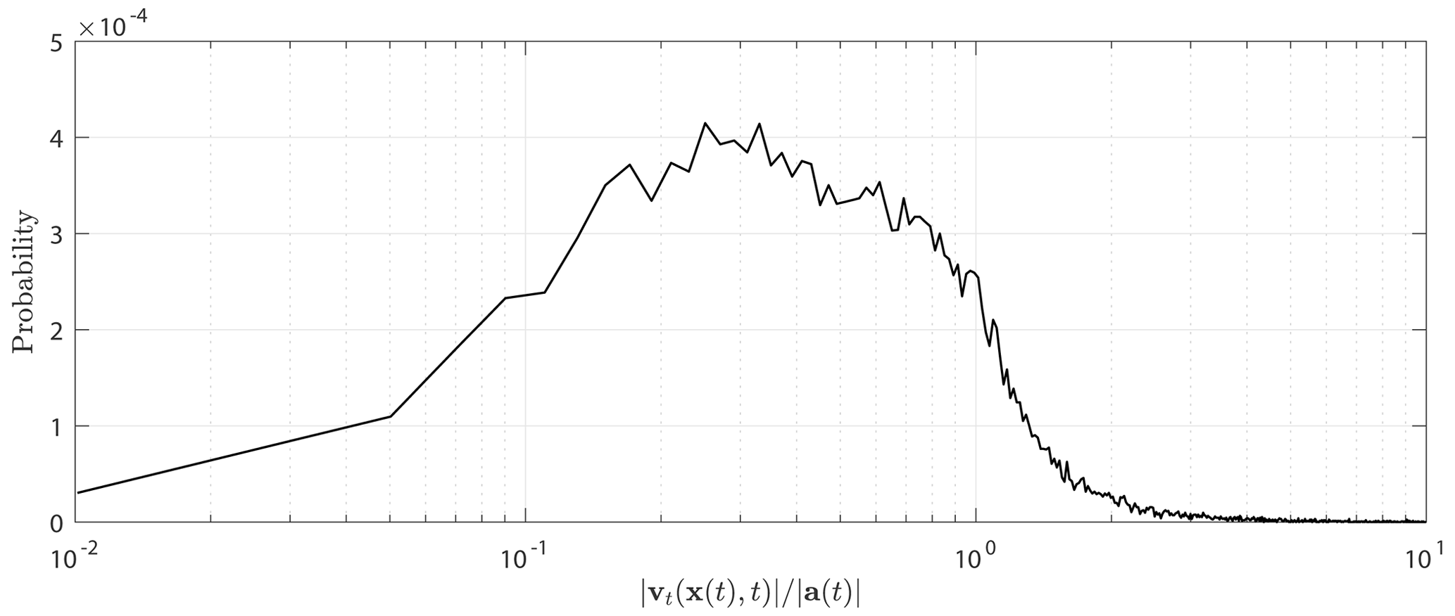
The TSE is a quasi-objective metric, indicating it approximates an objective metric under a given condition. For the work presented here, this requires that the velocity field of interest be slowly varying. That is, $\left|{\mathit{v}}_t\right(\mathit{x}\left(t\right),t\left)\right|\ll \left|\mathit{a}\right(t\left)\right|$, where a(t) is the Lagrangian velocity. In order to calculate the temporal derivative on the temporal derivative in v_t, we rely on daily gridded sea ice velocity data from Tschudi et al. (2018) as a best estimate for the flow. While one can calculate a(t) from trajectory data, discrete calculations of v_t(x(t),t) rely on repeat measurements of velocity at the same location. In this way, we require gridded velocity data to validate the slowly varying assumption.

The use of Pathfinder sea ice displacement grids comes with its own errors, such as the spatial gradient artifacts previously identified by Szanyi et al. (2016a). Furthermore, the low temporal resolution of this data smooths the short-time variability of surrounding instantaneous shear and fracture events. Prior to the development of a more robust gridded dataset of ice velocities, this remains the best available option.

The probability function in Fig. A7 shows that for the majority of the Arctic domain, the slowly varying condition is satisfied pointwise along sea ice trajectories. This probability is representative of midwinter ice conditions and may vary in the summer months. As this is a pointwise ratio, and not an integrated comparison, the slowly varying condition does not depend on a specific time window, the resolution of the underlying Pathfinder velocity field.

Figure A1 (a) Streamlines and velocity vectors for the geophysical Bickley jet. (b) The flow is designed to be divergence-free, as can be verified by a uniform divergence value of zero. (c) Instantaneous values of shear indicate strong shear zones adjacent to the top and bottom eddies and a narrow shear-free core. (d) Vorticity fields correctly identify the centers of the eddies above and below the jet. Note that the contours of shear do not agree with the shape of eddies in (a) and (d).

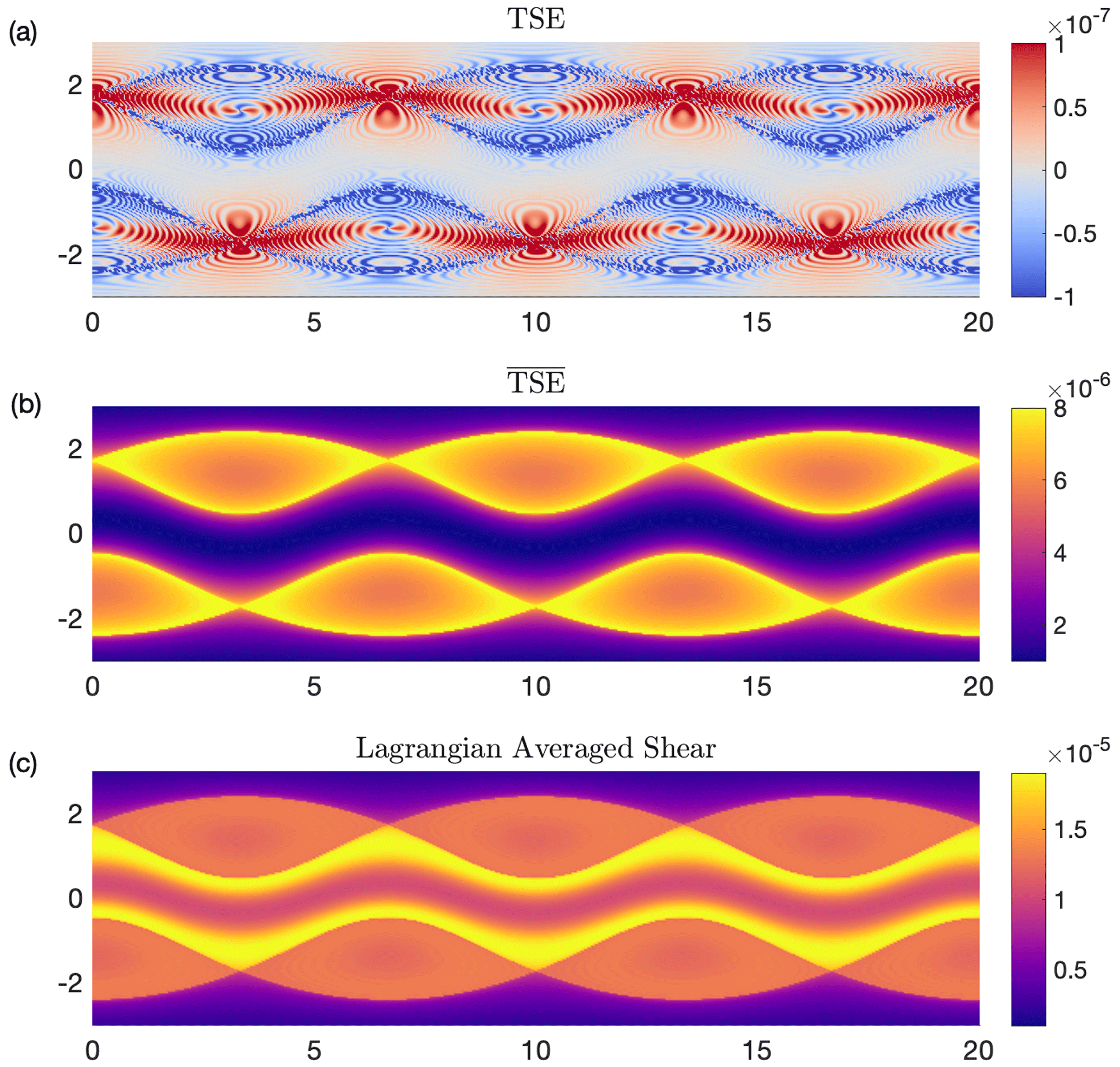
Figure A2 (a) TSE values show a complex stretch–relax pattern in the Bickley jet but still accurately identify the edges of each eddy as well as the central jet. (b) $\stackrel{\mathrm{‾}}{\mathrm{TSE}}$ contours clearly reveal the central jet and the adjacent eddies. There is limited trajectory-tangent stretching in the central jet, with a slight increase near the boundaries. (c) Lagrangian-averaged shear also reveals the multiple eddies and central jet, in contrast to Eulerian shear measurements. Lagrangian-averaged divergence is omitted as it is zero everywhere.

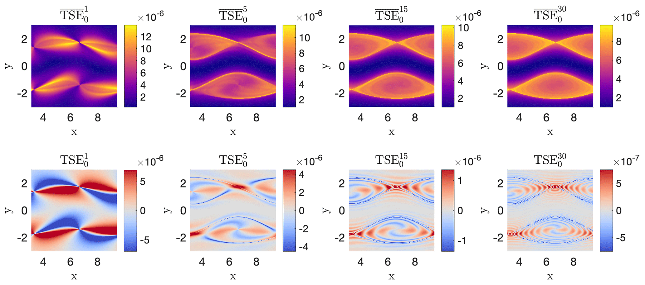
Figure A3 Comparison of TSE and $\stackrel{\mathrm{‾}}{\mathrm{TSE}}$ contours for increasing integration times from 1 to 30 d (L to R) for a subsection of the Bickley jet. The eddies, saddles between eddies, and central jet are evident for all integration times, but the clarity of boundaries increases as the integration time increases. Note this improvement is not always possible with time-dependent flows as features may change.

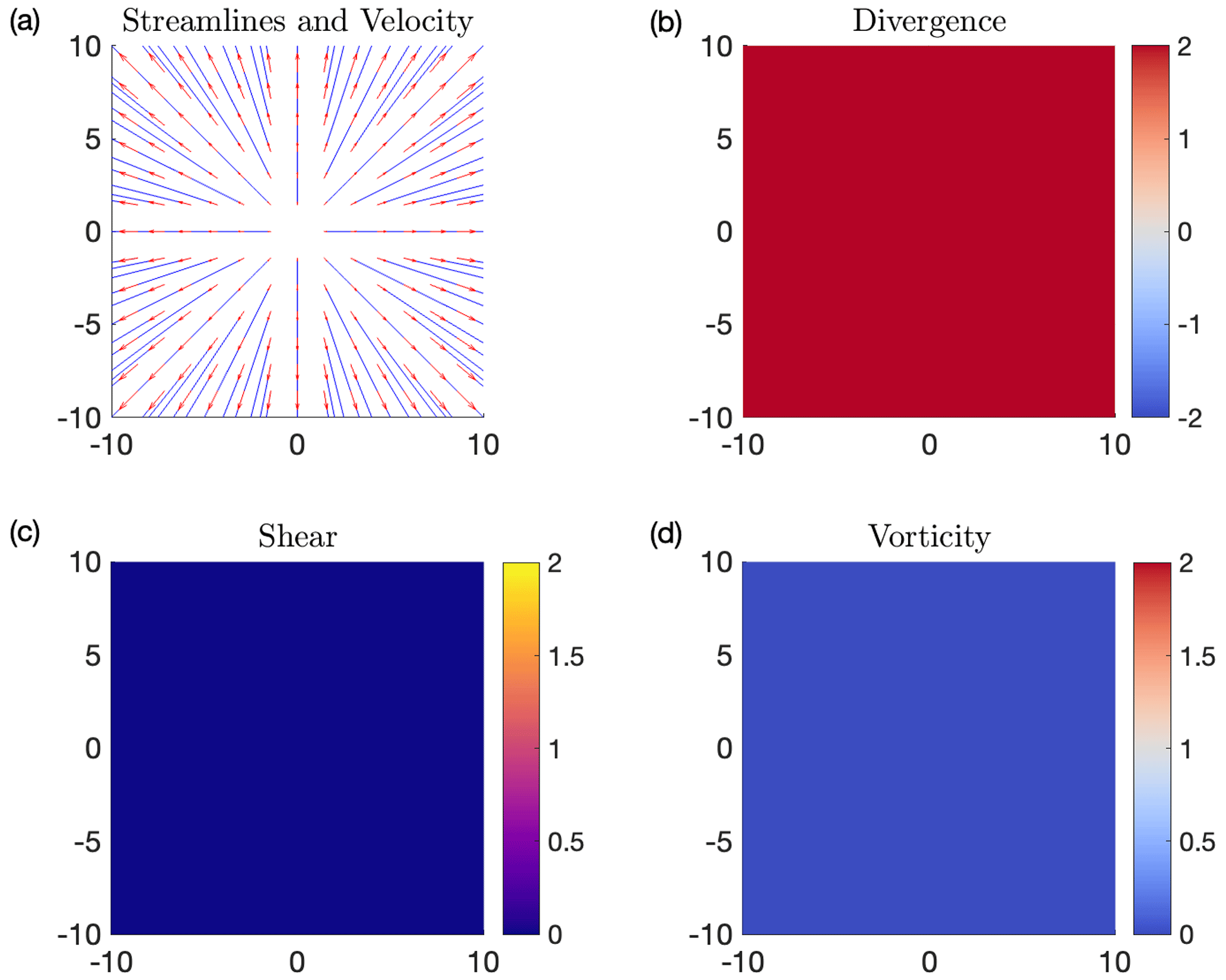
Figure A4 (a) Streamlines and velocity vectors for the divergent flow (Eq. A13). (b) The flow is designed to be uniformly divergent with a divergence value of 2. (c) Instantaneous values of zero shear. (d) Vorticity fields are also uniformly zero.

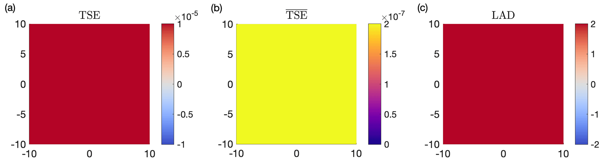
Figure A5 (a–b) TSEs and $\stackrel{\mathrm{‾}}{\mathrm{TSE}}$ show uniform stretching due to the uniform linear acceleration away from the origin. This matches the structure revealed by the uniform divergence field. (c) Lagrangian-averaged divergence is also constant, thus presenting the same pattern as TSEs and $\stackrel{\mathrm{‾}}{\mathrm{TSE}}$. The LS is omitted as it is constantly zero in this shear-free flow.

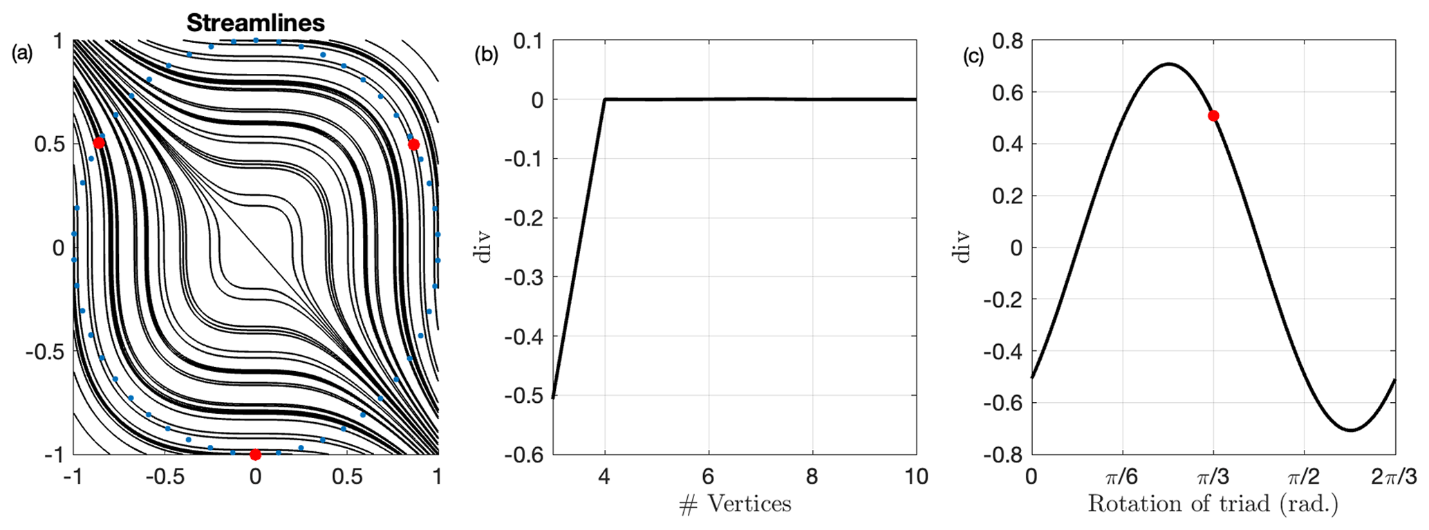
Figure A6 (a) Streamlines for the flow in Eq. (A14) with one example triad position (red) and unit circle of rotation (blue). (b) Average divergence as approximated by unit polygons as a function of the number of vertices used in the approximation. (c) Average divergence as approximated by a unit equilateral triad for all possible rotations, with divergence corresponding to (a) the triad in red.

Figure A7 Example assessment of the slowly varying assumption of Arctic sea ice velocities from Polar Pathfinder Daily 25 km EASE-Grid Sea Ice Motion Vectors, Version 4. $\left|{\mathit{v}}_t\right(\mathit{x}\left(t\right),t\left)\right|/\left|\mathit{a}\right(t\left)\right|$ calculated from 50 d of gridded sea ice trajectories surrounding the analysis in 2017 shown in Fig. 9.