the Creative Commons Attribution 4.0 License.
the Creative Commons Attribution 4.0 License.
 | 05 Apr 2023
A closed-form model for layered snow slabs
Philipp Weißgraeber
We propose a closed-form analytical model for the mechanical behavior of stratified snow covers for the purpose of investigating and predicting the physical processes that lead to the formation of dry-snow slab avalanches. We represent the system of a stratified snow slab covering a collapsible weak layer by a beam composed of an arbitrary number of layers supported by an anisotropic elastic foundation in a two-dimensional plane-strain model. The model makes use of laminate mechanics and provides slab deformations, stresses in the weak layer, and energy release rates of weak-layer anticracks in real time. The quantities can be used in failure models of avalanche release. The closed-form solution accounts for the layering-induced coupling of bending and extension in the slab and of shear and normal stresses in the weak layer. It is validated against experimentally recorded displacement fields and a comprehensive finite-element model indicating very good agreement. We show that layered slabs cannot be homogenized into equivalent isotropic bodies and reveal the impact of layering on bridging with respect to weak-layer stresses and energy release rates. It is demonstrated that inclined propagation saw tests allow for the determination of mixed-mode weak-layer fracture toughnesses. Our results suggest that such tests are dominated by mode I when cut upslope and comprise significant mode II contributions when cut downslope. A Python implementation of the presented model is publicly available as part of the Weak Layer Anticrack Nucleation Model (WEAC) software package under https://github.com/2phi/weac (last access: 28 March 2023) and https://pypi.org/project/weac (last access: 28 March 2023, Rosendahl and Weißgraeber, 2022).
- Article
(2292 KB) - Full-text XML
- BibTeX
- EndNote


Dry-snow slab avalanches are a critical danger in mountainous terrain with seasonal snow cover. Not only because of temporal succession of meteorological events are such seasonal covers composed of distinct individual layers. This yields snow covers that exhibit a stratification in terms of grain types, grain sizes, and density, among others, and consequently also mechanical properties. Highly fragile layers (e.g., depth hoar or buried surface hoar) are referred to as weak layers and are known to be the origin of slab avalanches (Bair, 2013). Their failure can lead to uncritical failure (whumpf sounds, shooting cracks) or avalanche release. The layering of snow covers is an essential part of avalanche forecasting (Richter et al., 2020) and for in-terrain decision making (Schweizer and Jamieson, 2007). It is known that the layering directly affects crack arrest or crack propagation (Birkeland et al., 2014). Hard layers within a snow slab have been identified as decisive for the effect of local load distribution within the snowpack (Schweizer et al., 1995; Camponovo and Schweizer, 1997).
Here, the so-called bridging effect that describes the load distribution through the slab onto lower layers as a function of slab and layer thicknesses has been found an important feature of the mechanics of snow covers (Schweizer and Camponovo, 2001b; Schweizer and Jamieson, 2003). The effects appears differently in crack propagation, where thicker slabs are linked to larger avalanches, and onset of avalanche failure, where thinner slabs are more critical (Jamieson and Johnston, 1998; van Herwijnen and Jamieson, 2007). This is also discussed in the experimental and numerical study on stress fields below localized loadings by Thumlert and Jamieson (2014).
When snow cover models are linked to stability analyses (see Morin et al., 2020, for a comprehensive review), typically stability indices are used (McClung and Schweizer, 1999; Lehning et al., 2004). These indices typically employ strength-based methods such as the limit equilibrium method (Föhn, 1987; Huang, 2014). Often, stress fields are obtained by using solutions derived from the Boussinesq solution of an infinite half-plane under a point load (Föhn, 1987; Gaume and Reuter, 2017). Monti et al. (2016) proposed an equivalent-layer approach to allow for the use of solutions of isotropic continua for the stress analysis of layered slabs. Since the early works of Smith and Chu (1972) and Smith and Curtis (1975), finite-element methods have been used to study stratified snowpacks (Schweizer, 1993; Habermann et al., 2008). These studies also clearly highlight the role of stratification and bridging on the stress and displacement fields within the snowpack.
The importance of bridging has been accounted for in the beam models by Heierli and Zaiser (2008) and Heierli et al. (2008). In these works, the concept of anticracks (Fletcher and Pollard, 1981) has been used to describe failure of weak layers in snow covers. Such beam models allowed for an insight into avalanche release and gave a physical explanation for whumpf sounds and remote triggering of avalanches, both caused by the sudden expansion of a local weak-layer collapse. Based on these models we have proposed a refined beam model for the analysis of stresses and energy release rates of cracks in weak layers (Rosendahl and Weißgraeber, 2020a). However, the above models are restricted to homogeneous slabs. The role of bending on anticrack formation and propagation (by collapse of weak layers) was also studied by means of the discrete-element method (Gaume et al., 2015; Bobillier et al., 2018). Gaume et al. (2018) investigated anticrack propagation in snow by means of an elastoplastic material model accounting for softening and volume reduction. Studying the effect of the slab properties on crack initiation and propagation, van Herwijnen and Jamieson (2007), Sigrist and Schweizer (2007), Habermann et al. (2008), and Reuter et al. (2015) have addressed the role of layering on fracture within snowpacks.
The importance of fracture mechanics for the analysis of avalanche release has been emphasized by many researchers (McClung, 1979, 1981; Heierli and Zaiser, 2006; Sigrist and Schweizer, 2007; Gauthier and Jamieson, 2008), and the significance of the fracture energy as the decisive material property has been highlighted (McClung and Schweizer, 2006; McClung, 2007; Heierli et al., 2008). In fracture-mechanics models the energy balance of propagating cracks is considered as the central condition for the analysis of avalanche release. Using Föhn's solution (Föhn, 1987) and the empirical measure of a critical crack length (Gaume et al., 2017), Gaume and Reuter (2017) have proposed to link strength-based approaches and fracture-mechanics approaches to assess the instability of snowpacks. Using an implicitly coupled stress and energy criterion we have proposed a failure model for anticrack initiation under mixed-mode loading that considers stresses and energy simultaneously (Rosendahl and Weißgraeber, 2020b).
In order to account for the crucial effect of layering on failure processes within a snowpack, we propose a new model for layered snow slabs on collapsible weak layers. Using the concepts of mechanics of layered composites (Jones, 1998) and weak interfaces (Lenci, 2001), we provide closed-form expressions that allow for real-time computations of snowpack deformations, weak-layer stresses, and the energy release rate of cracks in the weak layer. The work aims at establishing a fast computational framework for the physical analysis of the fracture process that leads to the formation of snow slab avalanches. For this purpose, the model considers discrete configurations of layered slabs supported by a weak layer that have collapsed on a given length. We to not attempt to formulate weak-layer failure criteria or to simulate crack advance but aim at providing the mathematical tools for such exercises.
In the present work, we model a stratified snow cover as a system comprised of (i) a snow slab, represented by an arbitrarily layered beam, that rests on (ii) a weak layer, represented by an elastic foundation. The beam kinematics and its constitutive behavior are derived from first-order shear deformation theory of laminated plates under cylindrical bending (Reddy, 2003). The weak layer is modeled as a so-called weak interface (Goland and Reissner, 1944). The concept simplifies the kinematics of the weak layer and allows for efficient analyses of interface configurations that exhibit a strong elastic contrast. The weak interface can be understood as an infinite set of smeared springs with normal and shear stiffness attached to the bottom side of the slab. Weak-interface models are common for the analysis of cracks in thin, compliant layers (Lenci, 2001; Krenk, 1992; Stein et al., 2015). The analysis of this system yields fully coupled bending, extension, and shear deformations of both the slab and the weak layer.
2.1 Governing equations
We consider a segment of the stratified snowpack on an inclined slope of angle φ as shown in Fig. 1. As typical for beam analyses, the axial coordinate x points left to right along the beam midplane and is zero at its left end. The thickness coordinate z is perpendicular to the midplane, points downwards, and is zero at the center line. Slope angles φ are counted positive about the y axis of the right-handed Cartesian coordinate system (counterclockwise). Note that on inclined slopes (φ≠0), the axial and normal beam axes (x and z) do not coincide with the horizontal and vertical directions.
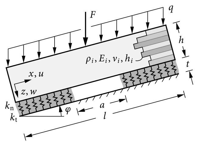
Figure 1Stratified snowpack composed of an arbitrary number of slab layers and a weak layer modeled as an elastic foundation.
The slab with total thickness h is composed of N layers with individual ply thicknesses , each assumed homogeneous and isotropic (Fig. 2). Young's modulus, Poisson's ratio, and the density of each layer are denoted by Ei, νi, and ρi, respectively. The weak layer of thickness t can be anisotropic, and its normal and tangential stiffnesses are
where is the weak layer's plane-strain elastic modulus, and
where Gwl is the weak layer's plane-strain shear modulus. To account for anisotropic weak layers, these constants can be defined from independent stiffness properties. It should be noted that since the weak layer is connected to the slab, an intrinsic coupling of shear and normal deformation of the weak layer occurs even when the stiffnesses kn and kt are defined independently.
The slab is loaded by its own weight, i.e., the gravitational load q, and an external load F (e.g., a skier) in vertical direction. The gravity load corresponds to the sum of the weight of all layers
It is split into a normal component qn=qcos φ and a tangential component , which are introduced as line loads. The tangential gravity line load acts at the center of gravity in the thickness direction,
in the slab, where yields each layer's center z coordinate. For relevant slab thicknesses the external load can be modeled as a point load and is introduced as a force with a normal component Fn=Fcos φ and a tangential component .
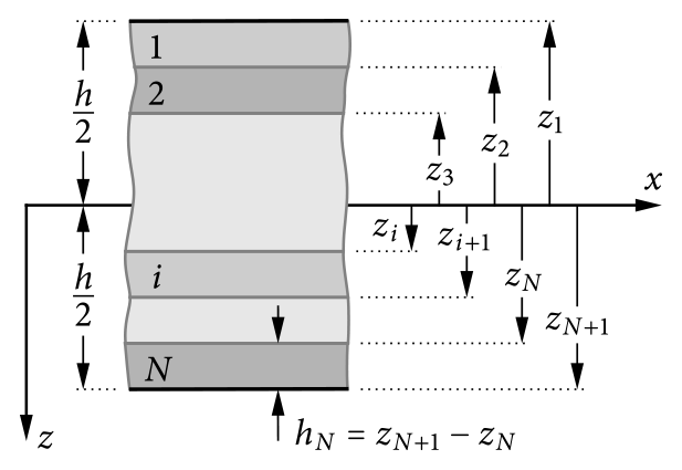
Figure 2Slab of total thickness h composed of N individual layers. A layer i is characterized by its height hi and its top and bottom coordinates zi and zi+1, respectively.
Deformations of the slab are described by means of the first-order shear deformation theory (FSDT) of laminated plates under cylindrical bending (Reddy, 2003). By dropping the Kirchhoff assumption of orthogonality of cross sections and midplane, this allows for the consideration of shear deformations. We consider midplane deflections w0, midplane tangential displacements u0, and the rotation ψ of cross sections. The quantities define the displacement field of the beam according to
At the interface between slab and weak layer (), the displacement fields of slab (u,w) and weak-layer (υ,ω) coincide. Using Eqs. (4a) and (4b), this yields and , where the bar indicates quantities at the interface. Modeling the weak layer as an elastic foundation of an infinite set of smeared linear elastic springs yields constant strains and consequently a constant deformation gradient through its thickness. Hence, weak-layer stresses can be expressed through the differential deformation between the lower boundary of the weak layer () and its deformations at the interface:
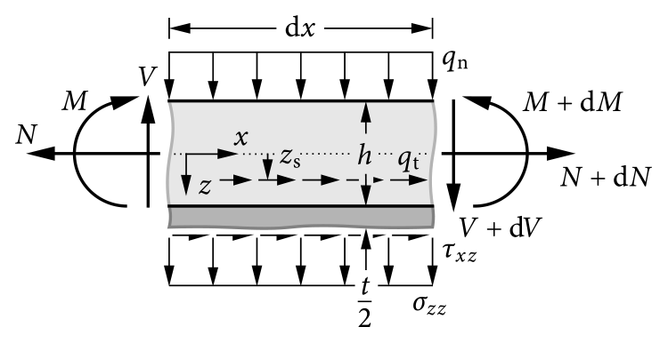
Figure 3Free-body cut of an infinitesimal segment of length of the layered slab of height with half of the weak layer.
From the free body-cut of an infinitesimal beam section of the layered slab (Fig. 3), we obtain the equilibrium conditions of the section forces and moments:
To connect the slab section forces (normal force N, shear force V, and bending moment M) to the deformations of the layered slab, we make use of the mechanics of composite laminates. The first-order shear deformation theory of laminate plates under cylindrical bending yields
and
These constitutive equations contain the extensional stiffness A11, the bending stiffness D11, the bending–extension coupling stiffness B11, and the shear stiffness κA55 of the layered slab. The coupling stiffness B11 accounts for the bending–extension coupling of asymmetrically layered systems such as bimetal bars. These stiffness quantities are obtained by weighted1 integration of the individual ply stiffness properties:
The shear correction factor κ complements the shear stiffness κA55. It is set to as a good approximation for the layered slab of rectangular cross section (Klarmann and Schweizerhof, 1993). The above quantities are given for the case of isotropic layers. Orthotropic layers can be considered following the same approach by using directional elastic properties of the individual layers instead of an isotropic Young modulus.
In the special case of a homogeneous, isotropic slab with Young's modulus Esl and Poisson's ratio ν, the laminate stiffnesses take the homogeneous stiffness properties well known from beam theory,
and the coupling stiffness vanishes (B11=0).
2.2 System of differential equations and its solution
The equations of the kinematics of the weak layer (Eqs. 5a and 5b), the equilibrium conditions (Eqs. 6a to 6c), and the constitutive equations of the layered beam with first-order shear deformation theory (Eqs. 7a and 7b) provide a complete description of the mechanics of the layered snowpack and constitute a system of ordinary differential equations (ODEs) of second order. Introducing the vector of unknown functions,
the governing equations can be expressed as a first-order system of the form
where bold uppercase symbols denote matrices and bold lowercase symbols indicate vectors. For the derivation of this ODE system and the definitions of the system matrix K and the right-hand side vector q, see Appendix A.
The solution of the nonhomogeneous ODE system (11) is composed of a complementary solution vector zh(x) and a particular integral vector zp, where the latter is constant in the present case. The complementary solution can be obtained from an eigenanalysis of the system matrix K. Depending on the layering and the material properties, K has six real or complex eigenvalues. Since the beam is bedded, it has no rigid body motions and all eigenvalues of nonzero. Real eigenvalues occur as sets of two eigenvalues with opposite signs ±λℝ and linearly independent eigenvectors . Complex eigenvalues appear as complex conjugates with the corresponding complex eigenvectors such that and . Denoting the number of sets of real eigenvalue pairs as and the number of complex conjugate eigenvalue pairs as such that , the complementary solution is given by the linear combination
The particular solution is obtained using the method of undetermined coefficients, which yields the constant vector
The general solution of the system,
comprises six unknown coefficients that must be identified from boundary and transmission conditions. It can be given in the matrix form
where is a matrix-valued function with the summands of Eq. (12) as column vectors and a vector containing the six free constants according of Eq. (12).
2.3 Layered segments without an elastic foundation
To study situations where the weak layer has partially failed, the case of an unsupported slab must be considered. The situation can occur when the weak layer has collapsed or when a saw cut is introduced in a propagation saw test. Accounting for such cases allows for the use of the present model in failure models for anticrack nucleation (Rosendahl and Weißgraeber, 2020b) or growth (Bergfeld et al., 2021b). If the slab is not supported by an elastic foundation, the general solution simplifies. In the equilibrium conditions (6a) to (6c), the normal and shear stress terms are omitted since no stresses act on the bottom side of the slab. The constitutive Eqs. (7a) and (7b) remain the same. After some calculation (see Appendix B) one obtains the general solution of polynomials of fourth order. In matrix form, the system reads
where 𝓟(x) and p(x) are the polynomial matrix and vector, respectively. Again, a vector of six unknown coefficients,
must be determined from boundary and transmission conditions.
2.4 Global system assembly
The general solutions presented above allow for the investigation of different systems composed of segments of supported and unsupported layered slabs. Possible configurations of interest are, e.g., skier-loaded snowpacks, skier-loaded snowpacks with a partially collapsed weak layer, or propagation saw tests (PSTs) with an artificially introduced (sawed) edge crack. Assemblies of such configurations are illustrated in Fig. 4. Individual segments are connected through transmission conditions given in terms of displacements and section forces (see Appendix C). Adding boundary conditions at the left and right ends of the beam assembles the desired global system. Since localized loads (e.g., skier weight) are introduced as a (statically equivalent) change of the section forces, the solution will not be able to fully render effects in the close vicinity of the load introduction. This is discussed in the validation in Sect. 3.2.
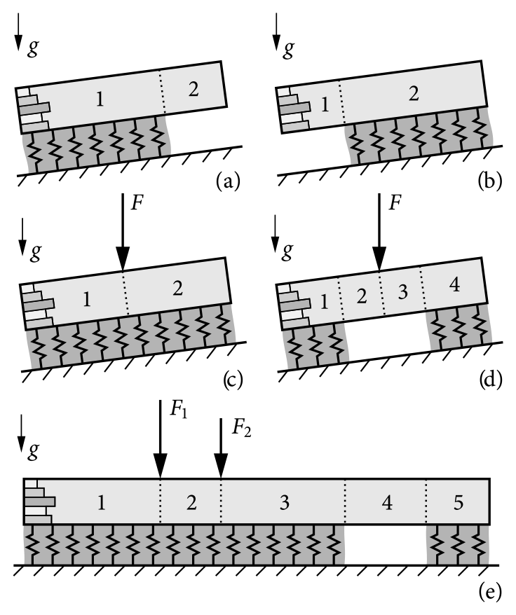
Figure 4Exemplary systems of interest assembled from supported and unsupported layered slabs with numbered segments: (a) downslope PST, (b) upslope PST, (c) skier-loaded snowpack, (d) partially fractured weak-layer, and (d) layered slab loaded by multiple skiers with partially fractured weak layer. Dotted lines indicate transmission conditions for the continuity of displacements and section forces.
Inserting the general solutions (15) and (16) into the boundary and transmission conditions yields equations that only depend on free constants. The set of equations can be assembled into a system of linear equations with k=6Nb degrees of freedom, where Nb is the number of beam segments. In matrix form, the system reads
Here, is a square matrix of full rank, c∈ℝk is the vector of all free constants, and f∈ℝk is the right-hand-side vector that contains the particular solutions and displacement discontinuities induced by concentrated loads. With only k degrees of freedom, the system can be solved in real time using standard methods such as Gaussian elimination or lower–upper (LU) decomposition.
2.5 Computation of displacements, stresses, and energy release rates
Substituting the coefficients C(n) obtained from Eq. (18) for each beam segment back into the general solutions (15) and (16) yields the vector z(x), which contains all slab displacement functions; see Eq. (10).
Inserting the slab deformation solution into Eqs. (5a) and (5b) provides weak-layer normal and shear stresses, respectively. As discussed in the details of the mechanical model, weak-interface models do not allow for capturing highly localized stress concentrations (e.g., stress singularities) as they occur at crack tips. However, it is known that outside the direct vicinity of crack tips, the simplified weak-interface kinematics provide accurate displacement and stress solutions (Rosendahl and Weißgraeber, 2020a).
The model can be used to determine the energy release rate of cracks. Here, we make use of the concept of anticracks (Fletcher and Pollard, 1981) that allows for studying failure of a weak layer in a snowpack exhibiting collapse (Heierli et al., 2008). As typical for fracture mechanics (Broberg, 1989), the symmetry of the displacement field around the crack tip can be used to identify symmetric (mode I) and antisymmetric deformations (mode II). We follow this convention to study mode I (crack closure) and mode II (crack sliding) energy release rates of anticracks. Further implications are discussed in Rosendahl and Weißgraeber (2020b). Following Krenk (1992), the energy release rate of cracks in weak interfaces can be given as
where a denotes the crack-tip coordinate. The limitations of the weak-interface kinematics yield energy release rates that cannot capture very short cracks but, again, provide accurate results for cracks of a minimum length (Hübsch et al., 2021). Cracks shorter than a few millimeters cannot be studied by the present approach.

Figure 5Illustration of benchmark snow profiles used in the present work. Material properties of hard, medium, and soft slab layers (dark) and the weak layer (light) are given in Table 1. The weak layer is 2 cm thick and the slab layers have a thickness of 12 cm each. Similar profiles were used by, e.g., Habermann et al. (2008) and Monti et al. (2016). Here, we complement the homogeneous slab H.
Table 1Considered snow layers and their elastic properties with reference to three-layer slabs used by Habermann et al. (2008).
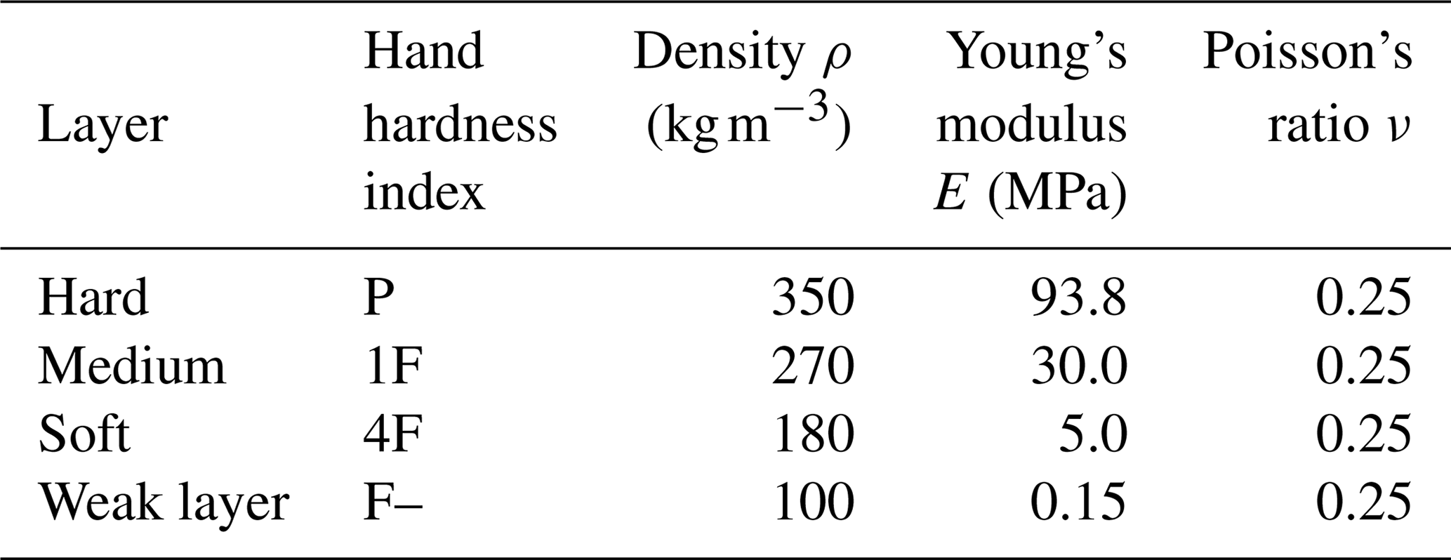
With reference to the analysis of snowpack layering by Habermann et al. (2008) and Monti et al. (2016), we use three-layered slabs proposed as schematic hardness profiles by Schweizer and Wiesinger (2001) that are composed of soft, medium, and hard snow as benchmark slab configurations (Fig. 5). Assuming bonded slabs (e.g., rounded grains) and considering the density–hand-hardness relations given by Geldsetzer and Jamieson (2000), we assume densities of ρ=350, 270, and 180 kg m−3 for hard, medium, and soft snow layers with hand hardness indices pencil (P), four fingers (4F), and one finger (1F), respectively. From slab densities, we calculate Young's modulus using the density parametrization developed by Gerling et al. (2017) using acoustic wave propagation experiments and improved by Bergfeld et al. (2023a) using full-field displacement measurements:
where ρ0=917 kg m−3 is the density of ice. Each slab layer is 12 cm thick, and their individual material properties are given in Table 1. With reference to Jamieson and Schweizer (2000), who report weak layer thickness between 0.2 and 3 cm, we assume a weak-layer thickness of t=2 cm. Following density measurements of surface-hoar layers by Föhn (2001), who reports densities (i) between 44 and 215 kg m−3 with a mean of 102.5 kg m−3 and (ii) between 75 and 252 kg m−3 with a mean of 132.4 kg m−3 using two different measurement techniques, we assume a weak-layer density of ρwl=100 kg m−3 and a Young modulus of Ewl=0.15 MPa. Other parameters are summarized in Table 2.
Table 2Material properties used throughout this work unless specified differently.

* Thicknesses given in slope-normal direction.
3.1 Finite-element reference model
To validate the model, in particular with respect to different slab layerings, we compare the analytical solution to finite-element analyses (FEAs). The finite-element model is assembled from individual layers with unit out-of-plane width on an inclined slope. Each layer is discretized using at least 10 eight-node biquadratic plane-strain continuum elements with reduced integration through its thickness. The lowest layer corresponds to the weak layer and rests on a rigid foundation. Weak-layer cracks are introduced by removing all weak-layer elements on the crack length a. The mesh is refined towards stress concentration such as crack tips, and mesh convergence has been controlled carefully (Rosendahl and Weißgraeber, 2020a). The weight of the snowpack is introduced by providing the gravitational acceleration g and assigning each layer its corresponding density ρ. The load introduced by a skier is modeled as a concentrated force acting on the top of the slab. If skier loading is considered, the horizontal dimensions of the model are chosen large enough for all gradients to vanish. Typically 10 m suffice. Boundary conditions of PST experiments are free ends. In the FE model, the energy release rate of weak-layer cracks,
is computed using the central difference quotient to approximate the first derivative of the total potential Π with respect to a. The crack increment Δa corresponds to the element size and could be increased 2-fold or 3-fold without impacting computed values of 𝒢FE(a). Weak-layer stresses are evaluated in its vertical center.
3.2 Visualization of displacement and stress fields
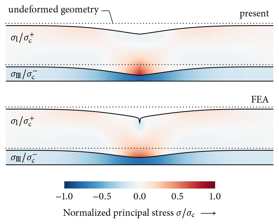
Figure 6Principal stresses and snowpack deformations scaled 200 times in the central 200 cm section of a skier-loaded snowpack comparing the present model (top) and the FEA reference model (bottom). In the homogeneous slab ![]() H, maximum principal normal stresses σI (tension) normalized to their tensile strength kPa are shown. In the weak layer we show minimum principal normal stresses σIII (compression) normalized to an assumed weak layer compressive strength of kPa. The weak-layer thickness is scaled by a factor of 4 for illustration.
H, maximum principal normal stresses σI (tension) normalized to their tensile strength kPa are shown. In the weak layer we show minimum principal normal stresses σIII (compression) normalized to an assumed weak layer compressive strength of kPa. The weak-layer thickness is scaled by a factor of 4 for illustration.
Although visual representations of deformation and stress fields are limited to qualitative statements, they illustrate the principal responses of structures in different load cases. For this purpose, Fig. 6 compares principal stresses in a deformed slab-on-weak-layer system between the present model and the finite-element reference solution. The system is loaded by the weight of the homogeneous slab ![]() H and a concentrated force representing an 80 kg skier. Deformations are scaled by a factor of 200 and the weak-layer thickness by a factor of 4. In the slab, we show maximum principal normal stresses (tension) normalized to their tensile normal strength obtained from the scaling law
H and a concentrated force representing an 80 kg skier. Deformations are scaled by a factor of 200 and the weak-layer thickness by a factor of 4. In the slab, we show maximum principal normal stresses (tension) normalized to their tensile normal strength obtained from the scaling law
by Sigrist (2006), where is the density of ice. This illustrates the potential of tensile slab fracture. In the weak layer, minimum principal normal stresses (compression) normalized to their rapid-loading compressive strength kPa according to Reiweger et al. (2015) are shown, illustrating the potential for weak-layer collapse. We choose principal stresses for the visualization because they allow for the assessment of complex stress states by incorporating several stress components. Please refer to Appendix D for the calculation of principal stresses from model outputs.
While the present model (Fig. 6, top panel) does not capture the highly localized stresses at the contact point between skier and slab observed in the FEA model (Fig. 6, bottom panel), the overall stress fields are in excellent agreement. This is consistent with Saint-Venant's principle, according to which the far-field effect of localized loads is independent of their asymptotic near-field behavior. The same holds for the displacement field. While the concentrated load introduces a dent in the slab's top surface, the overall deformations agree. With respect to the numerical reference, the present model renders displacement fields and both weak-layer and slab stresses well. Moreover, we can confirm the model assumption of constant stresses through the thickness of the weak layer.
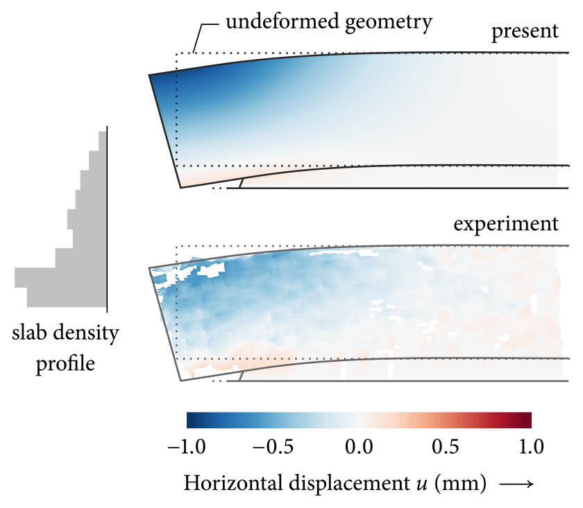
Figure 7Horizontal displacement field of the first 1.3 m of a flat-field propagation saw test (PST) with an a=23 cm cut into the t=1 cm weak layer under an h=46 cm slab. Comparison of the present model (top) with full-field digital image correlation measurements (bottom). White patches indicate missing data points. Deformations are scaled by a factor of 100 and the weak-layer thickness by a factor of 10 for illustration.
Experimental validations are challenging since direct measurements of stresses are not possible and displacement measurements require considerable experimental effort. The latter can be recorded using digital image correlation (DIC) as demonstrated by Bergfeld et al. (2023a). From their analysis, we use the DIC-recorded displacement field of the first 1.3 m of a 3.0±0.1 m long flat-field propagation saw test (Fig. 7, bottom panel). The PST was performed on 7 January 2019, had a slab thickness of h=46 cm, a critical cut length of , and the density profile shown in Fig. 7 (left panel) with a mean slab density of . From the density we computed individual layer stiffnesses according to Eq. (20). Figure 7 compares both in-plane deformations of the snowpack (outlines) and the horizontal displacement fields (colorized overlay) obtained from the present model (top panel) and from DIC measurements (bottom panel). Deformations are scaled by a factor of 100 and the weak-layer thickness by a factor of 10 for their visualization. In-plane slab and weak-layer deformations are in very good agreement. This is evident in both the deformed contours and in the colorized displacement field overlay. Since displacements are 𝒞1 continuous across layer interfaces, the effect of layering is not directly visible in the displacement field. However, the slightly larger-than-expected tilt of the slab at its left end hints at a higher stiffness at the bottom of the slab and a compliant top section.
3.3 Weak-layer stresses and energy release rates
For all benchmark profiles illustrated in Fig. 5, weak-layer shear and normal stresses (τ,σ) obtained from the FEA model (dotted, light) and the present analytical solution (solid, dark) are compared in Fig. 8. We investigate a 38∘ inclined slope subjected to a concentrated force equivalent to the load of an 80 kg skier on an effective out-of-plane ski length of 1 m. The finite-element reference model has a horizontal length of 10 m, of which the central 3 m is shown. The boundary conditions of the present model require the complementary solution (12) to vanish, representing an infinite extension of the system.
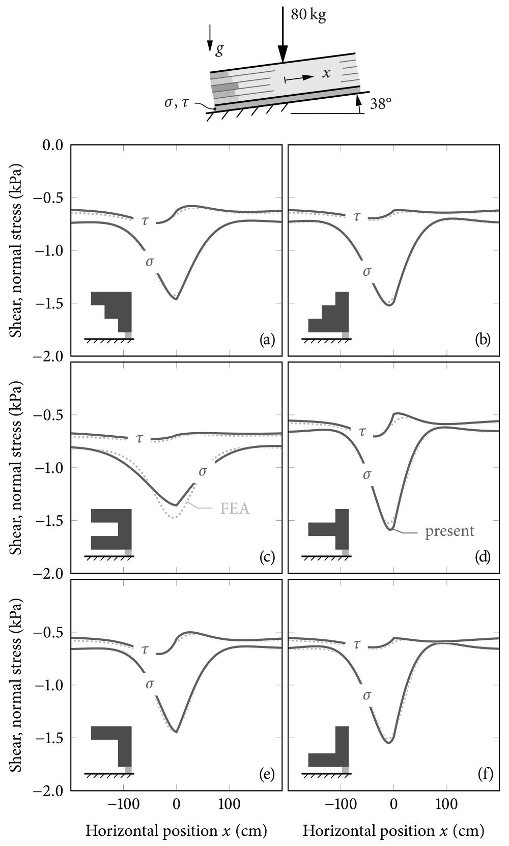
Figure 8Weak-layer normal and shear stresses (σ,τ) owing to combined skier and snowpack-weight loading for the benchmark profiles illustrated in Fig. 5. The present solution
(solid, dark) only slightly underestimates the maximum normal stresses with respect to the FEA reference (dotted, light) in the case of profile
![]() C. Material properties are given in Tables 1 and 2.
C. Material properties are given in Tables 1 and 2.
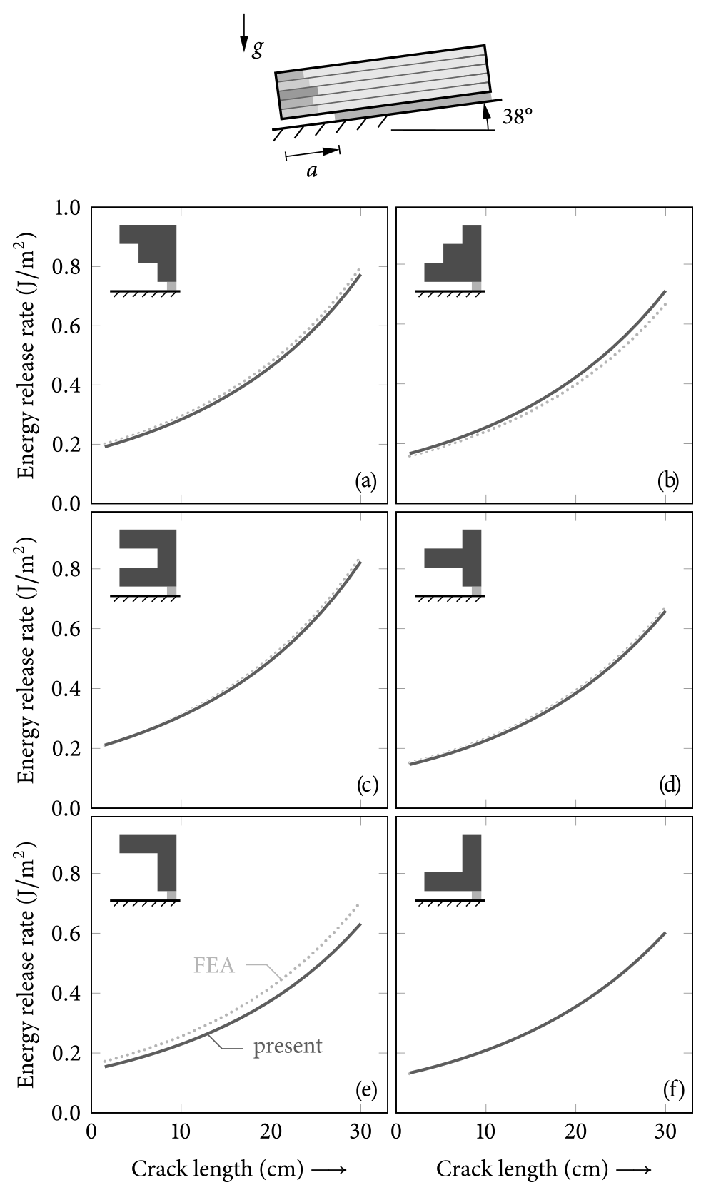
Figure 9Total energy release rates of weak-layer anticracks in 38∘ inclined PST experiments of 120 cm length with the benchmark profiles illustrated in Fig. 5. The present solution (solid, dark) and FEA reference (dotted, light) are in good agreement. Material properties are given in Tables 1 and 2.
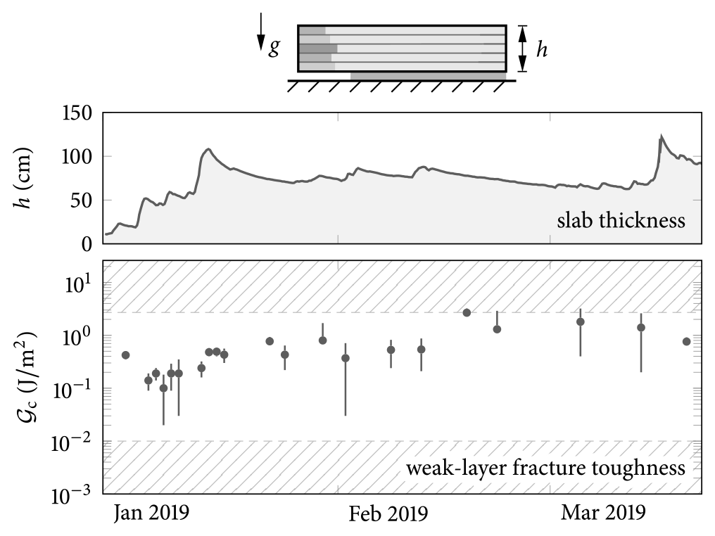
Figure 10Weak-layer fracture toughness determined with the present model from critical cut lengths of 21 flat-field propagation saw tests (PSTs) throughout the 2019 winter season on the same surface-hoar weak layer covered by a layered slab of changing thickness (Bergfeld et al., 2023a, b). All results are within the hatched boundaries, indicating the thus far lowest and highest published fracture toughness of weak layers, 0.01 J m−2 (Gauthier and Jamieson, 2010) and 2.7 J m−2 (van Herwijnen et al., 2016), respectively.
Kinks in the model solution originate from the loading discontinuity introduced by the concentrated skier force. They are a direct result of the plate-theory modeling approach. The agreement with the FEA reference solution is close for all types of investigated profiles, and layering effects on weak-layer stress distributions are well captured. Only for profile ![]() C does the present solution slightly underestimate the normal stress peak directly below the skier. As we argue in Rosendahl and Weißgraeber (2020b), this observation is not relevant for the prediction of weak-layer failure in a snow cover. To study size effects present in any structure, a nonlocal evaluation of stresses must be used (Neuber, 1936; Peterson, 1938; Waddoups et al., 1971; Sih, 1974). This has been discussed in detail by Leguillon (2002), laying the foundation for the successful application of finite-fracture-mechanics approaches with weak-interface models (Weißgraeber et al., 2015; Rosendahl et al., 2019).
Effects of bending stiffness (Fig. 8c vs. d) or bending–extension coupling (Fig. 8e vs. f) resulting from different layering orders will be discussed in detail below.
C does the present solution slightly underestimate the normal stress peak directly below the skier. As we argue in Rosendahl and Weißgraeber (2020b), this observation is not relevant for the prediction of weak-layer failure in a snow cover. To study size effects present in any structure, a nonlocal evaluation of stresses must be used (Neuber, 1936; Peterson, 1938; Waddoups et al., 1971; Sih, 1974). This has been discussed in detail by Leguillon (2002), laying the foundation for the successful application of finite-fracture-mechanics approaches with weak-interface models (Weißgraeber et al., 2015; Rosendahl et al., 2019).
Effects of bending stiffness (Fig. 8c vs. d) or bending–extension coupling (Fig. 8e vs. f) resulting from different layering orders will be discussed in detail below.
A similar comparison of solutions for all profiles is given in Fig. 9, where total energy release rates (ERRs) of weak-layer anticracks in 38∘ inclined PST experiments are shown. Here, both models consider free boundaries of the 1.2 m long PST block. The structure is loaded by the weight of the slab, and saw-introduced cracks are modeled by removing all weak-layer elements on the crack length a. This causes finite ERRs, even for very small cracks, because a finite amount of strain energy is removed from the system with these elements. The ERR of a sharp crack is expected to vanish in the limit of zero crack length (≪1 cm).
The principal behavior of the ERR as a function of crack length is unaffected by the choice of profile. However, the different resulting stiffness and deformation properties influence the magnitude of the energy release rate considerably. For instance, between cases A and B, we observe a difference of almost 10 % (Fig. 9).
Figure 10 shows weak-layer fracture toughnesses determined from critical cut lengths of PSTs with layered slabs throughout the 2019 winter season using the present model. Details of the tests are reported by Bergfeld et al. (2023a, b). The authors performed 21 tests on the same weak layer. While we observe small weak-layer fracture toughnesses at the beginning of January 2019, it quickly increases with the most significant precipitation event in mid-January and then remains comparatively constant throughout the rest of the season. For details on the temporal evolution of slab and weak-layer properties, the interested reader can refer to Bergfeld et al. (2023b). For the purpose of validation of the present model, it should be noted that all fracture toughnesses computed from the experiments lie within the bounds of the to-date lowest and highest published values, 0.01 J m−2 (Gauthier and Jamieson, 2010) and 2.7 J m−2 (van Herwijnen et al., 2016), respectively.
The present model can be classified as a structural-mechanics model as frequently employed in fracture mechanics. As shown by Bergfeld et al. (2021b), structural models can be used to obtain effective quantities characterizing weak layers. Effective quantities of fracture-mechanics models always include microscopic mechanisms without further resolving their microscopic nature (Broberg, 1989).
In the following, we use the above model to conduct parametric studies in order to investigate key mechanisms that may or may not lead to the release of slab avalanches. Among these are bridging or the effect of layer ordering. Unless specified otherwise, we used the material parameters given in Tables 1 and 2.
4.1 Stiffnesses of layered slabs
The mechanical behavior of the slab is governed by its stiffnesses. A layered system may have different stiffnesses with respect to extension, shear, or bending. Hence, we distinguish the extensional stiffness A11, the bending–extension coupling stiffness B11, the bending stiffness D11, and the shear stiffness A55. They are obtained from integration of the individual layer stiffnesses as specified in Eqs. (8a) to (8d). The ordering of layers influences each stiffness differently. That is, the simple homogenization of layered continua in the form of a single homogeneous equivalent layer is insufficient. With the aim to describe the shear stresses in a slab, Monti et al. (2016) proposed a concept of equivalent layers to allow for the use of Boussinesq's solution for an isotropic elastic half-plane. They followed concepts developed in order to describe the surface deformation of layered systems in the normal direction (De Barros, 1966). Using the equivalent Young modulus Eeq introduced by Monti et al. (2016), the stiffnesses of a homogenized slab read
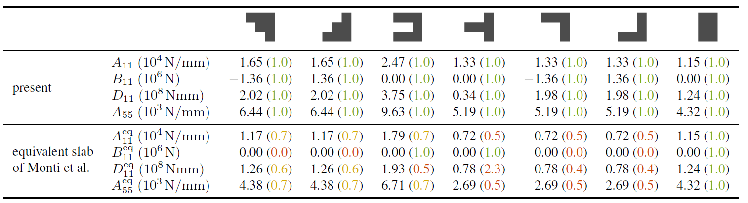
Table 3 and Fig. 11 compare stiffnesses computed with the present concept of laminate mechanics, Eqs. (8a) to (8d), with these stiffnesses of an equivalent homogeneous slab computed with properties obtained from the equivalence concept, Eqs. (23a) to (23d). Table 3 and Fig. 11 compare both concepts against the stiffnesses computed using finite-element analyses. Here, the corresponding stiffnesses are obtained from the force response of unit extension and bending deformations. While Eqs. (8a) to (8d) reproduce the reference stiffnesses exactly, the equivalent layer approach systematically underestimates the extensional, the bending, and the shear stiffnesses and cannot account for bending–extension couplings.

Figure 11Slab extension, bending, and shear stiffnesses A11 (N mm−1), D11 (N mm), and A55 (N mm−1) of the present model and the equivalent isotropic slab approach by Monti et al. (2016) normalized to the finite-element analysis (FEA) reference stiffness. The bending–extension coupling stiffness B11 (N) is not shown because it is always zero in the model of Monti et al. (2016) and agrees exactly between reference and present model; see Table 3.
Table 3Slab extension, coupling, bending, and shear stiffnesses of the benchmark profiles. Comparison of A11,B11, D11, and A55 of the present model with , , and obtained from an equivalent isotropic slab according to Monti et al. (2016). Numbers in parentheses indicate the ratio of the modeled stiffness to the corresponding stiffness obtained from finite-element analyses (visualized in Fig. 11). Layer configurations as detailed in Fig. 5 are used.
4.2 Effect of layering
To study the effect of layering we look at the deformations within a PST of 250 cm length with a 50 cm cut (20% of the PST length). The symmetric configuration of profile ![]() C is studied as well as the profiles
C is studied as well as the profiles
![]() A and
A and
![]() B with typical layerings. The results are shown in Fig. 12. Here, the unsupported length of the slab is illustrated by a shaded background. The longitudinal displacement of the midplane u0 and at the interface between the slab and the weak layer shows pronounced effects around the crack tip that induces slab bending. The midplane deformation of the symmetric profile
B with typical layerings. The results are shown in Fig. 12. Here, the unsupported length of the slab is illustrated by a shaded background. The longitudinal displacement of the midplane u0 and at the interface between the slab and the weak layer shows pronounced effects around the crack tip that induces slab bending. The midplane deformation of the symmetric profile ![]() C is practically unaffected by this bending since its bending–extension stiffness B11 is zero (Table 3). That is, bending and extension are only coupled through the weak layer but not through the slab itself. The near-constant midplane displacements originate from the 38∘ inclination. For the asymmetric profiles, the effect of slab bending depends on the stiffness distribution. The stiff bottom layer of profile
C is practically unaffected by this bending since its bending–extension stiffness B11 is zero (Table 3). That is, bending and extension are only coupled through the weak layer but not through the slab itself. The near-constant midplane displacements originate from the 38∘ inclination. For the asymmetric profiles, the effect of slab bending depends on the stiffness distribution. The stiff bottom layer of profile ![]() B increases midplane displacements when the slab bends down on towards the right end of the PST. The opposite is observed for profile
B increases midplane displacements when the slab bends down on towards the right end of the PST. The opposite is observed for profile ![]() A with a stiff top layer. Here, the midplane displacements are reduced owing to crack-induced slab bending. The effect can be attributed to the different signs of the bending–extension stiffnesses B11 of profiles
A with a stiff top layer. Here, the midplane displacements are reduced owing to crack-induced slab bending. The effect can be attributed to the different signs of the bending–extension stiffnesses B11 of profiles ![]() A and
A and ![]() B (Table 3). Constant longitudinal displacements at the interface between slab and weak layer are reduced by slab bending for all profiles. Profile
B (Table 3). Constant longitudinal displacements at the interface between slab and weak layer are reduced by slab bending for all profiles. Profile ![]() C has the largest bending stiffness D11 (Table 3). Hence, its reduction of is smallest. Again, the stiff top layer of profile
C has the largest bending stiffness D11 (Table 3). Hence, its reduction of is smallest. Again, the stiff top layer of profile ![]() A causes a strong reduction of axial displacements.
Deflections w0 are downward positive (compression of the weak layer) along the complete PST and increase towards the cut end. Again, profile
A causes a strong reduction of axial displacements.
Deflections w0 are downward positive (compression of the weak layer) along the complete PST and increase towards the cut end. Again, profile ![]() C has the largest bending stiffness and, hence, exhibits the smallest deflections. Soft top layers (profile
C has the largest bending stiffness and, hence, exhibits the smallest deflections. Soft top layers (profile ![]() B) cause the largest deflections. Cross-section rotations ψ are close to zero in the longitudinal center of the PST and increase towards the free ends of the PST, where the negative sign indicates down bending. Similar arguments as for w0 hold.
B) cause the largest deflections. Cross-section rotations ψ are close to zero in the longitudinal center of the PST and increase towards the free ends of the PST, where the negative sign indicates down bending. Similar arguments as for w0 hold.
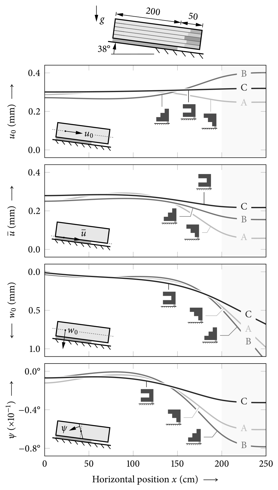
Figure 12Deformations along the length of a PST with a cut at x=200 cm (cut length 50 cm) illustrated by the shaded background. Comparison of three snow profiles. The longitudinal displacement of the midplane of the slab u0 and at the interface between slab and weak layer , the deflection w0, and the cross-section rotation ψ are shown.
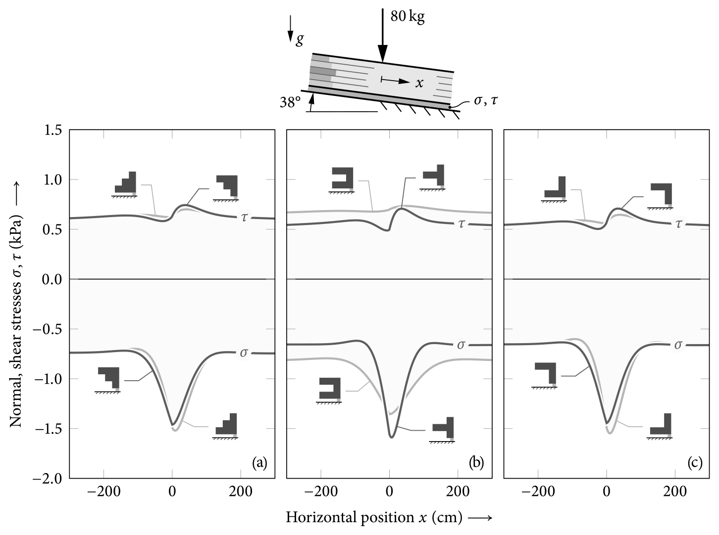
Figure 13Comparison of shear and normal stresses in the weak layer of inclined skier-loaded layered snowpacks. The central 0.6 m section of an infinite slab is shown.
The effect of layering on the stresses in the weak layer is illustrated in Fig. 13. It shows shear and normal stresses in the weak layer below a skier-loaded slab – each panel for two of the considered profiles. Since the profiles ![]() A and
A and ![]() B and profiles
B and profiles
![]() E and
E and
![]() F have the same mean densities, their stress levels outside the skier's influence zone are the same. Profiles
F have the same mean densities, their stress levels outside the skier's influence zone are the same. Profiles ![]() C and
C and
![]() D have a different mean densities, and, hence, the stresses induced by the slab weight outside the skier's influence are different. Here, constant loading leads to constant slab deformations and, hence, to constant weak layer stresses. Both shear and normal stresses show pronounced stress peaks close to the skier load point. As discussed above (Table 3), owing to their layering, profiles
D have a different mean densities, and, hence, the stresses induced by the slab weight outside the skier's influence are different. Here, constant loading leads to constant slab deformations and, hence, to constant weak layer stresses. Both shear and normal stresses show pronounced stress peaks close to the skier load point. As discussed above (Table 3), owing to their layering, profiles ![]() C and
C and ![]() D differ significantly in their bending stiffnesses (factor of 11) while the extensional stiffness is only doubled. In particular the smaller bending stiffness of profile
D differ significantly in their bending stiffnesses (factor of 11) while the extensional stiffness is only doubled. In particular the smaller bending stiffness of profile ![]() D leads to localized stresses below the skier with higher maximum values but narrower influence zones (Fig. 13b). In the comparison of profiles
D leads to localized stresses below the skier with higher maximum values but narrower influence zones (Fig. 13b). In the comparison of profiles ![]() A and
A and ![]() B (Fig. 13a) and profiles
B (Fig. 13a) and profiles ![]() E and
E and ![]() F (Fig. 13c), we observe that profiles with increasing top-to-bottom stiffness exhibit slightly stronger weak-layer normal stress concentrations but weaker shear stress concentrations compared to their counterparts with reverse layering order.
F (Fig. 13c), we observe that profiles with increasing top-to-bottom stiffness exhibit slightly stronger weak-layer normal stress concentrations but weaker shear stress concentrations compared to their counterparts with reverse layering order.
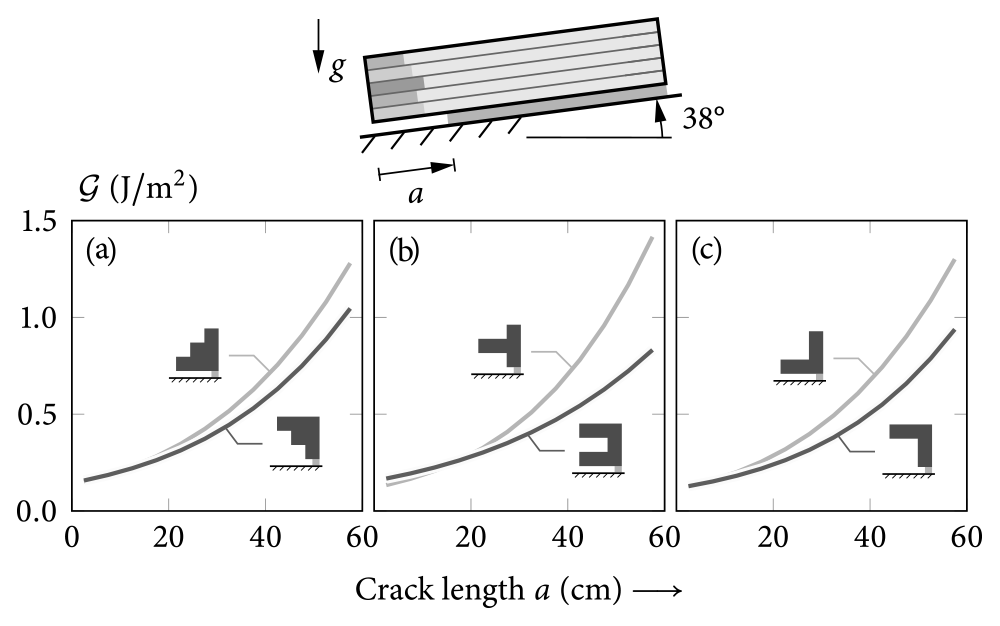
Figure 14Comparison of total differential energy release rates 𝒢 of cracks of length a in a 2.5 m long PST between the considered benchmark profiles.
In Fig. 14, the energy release rates of cuts introduced in PST experiments are shown as a function of crack length. For each pair of two profiles (A–B, C–D, E–F), the total differential energy release rate is shown. All curves show the expected monotonic increase in the energy release rate with increasing crack length. However, magnitudes and the progression towards higher crack lengths strongly depend on the layering. The comparisons of profiles ![]() A vs.
A vs. ![]() B (Fig. 14a) and
B (Fig. 14a) and ![]() E vs.
E vs. ![]() F (Fig. 14c) illustrate that even with same extensional and bending stiffnesses, the order of layers has a significant impact on the energy released during crack growth. As observed in Fig. 13, profiles with increasing top-to-bottom stiffness are more critical with respect to the weak layer's structural integrity. The energy release rate depends both on the compliance of the snowpack and on the overall loading. That is, layers of higher density represent increased weight loads, but since the Young modulus increases with increasing stiffness, deformations of the slab and energy release rates may decrease. This is evident in Fig. 14b. Here, profile
F (Fig. 14c) illustrate that even with same extensional and bending stiffnesses, the order of layers has a significant impact on the energy released during crack growth. As observed in Fig. 13, profiles with increasing top-to-bottom stiffness are more critical with respect to the weak layer's structural integrity. The energy release rate depends both on the compliance of the snowpack and on the overall loading. That is, layers of higher density represent increased weight loads, but since the Young modulus increases with increasing stiffness, deformations of the slab and energy release rates may decrease. This is evident in Fig. 14b. Here, profile ![]() C is heavier than profile
C is heavier than profile ![]() D. However, owing to its increased stiffness, its energy release rate is smaller.
D. However, owing to its increased stiffness, its energy release rate is smaller.
4.3 Bridging
The distribution of a localized external load over a certain area of the weak layer (bridging) depends on the stiffness of the slab. To study this important effect, Fig. 15 shows skier-induced weak-layer stresses below a slab with profile ![]() F in its original and a modified configuration. For the modification, the thicknesses of all layers of the original profile given in Table 1 are halved. The reduced weight (ρ∝h) of the thinner slab leads to smaller overall stresses. However, its reduced stiffness () yields more pronounced stress peaks. In the case of normal stresses, peak compressive stresses below the thinner slab even exceed the ones of the original configuration. For shear stresses, the sharper stress peak does not outweigh the reduced slab weight.
F in its original and a modified configuration. For the modification, the thicknesses of all layers of the original profile given in Table 1 are halved. The reduced weight (ρ∝h) of the thinner slab leads to smaller overall stresses. However, its reduced stiffness () yields more pronounced stress peaks. In the case of normal stresses, peak compressive stresses below the thinner slab even exceed the ones of the original configuration. For shear stresses, the sharper stress peak does not outweigh the reduced slab weight.
While the effect of bridging on weak-layer stresses through the distribution of concentrated loads is somewhat intuitive, it can be observed for the energy release rate of weak-layer anticracks, too. Let us demonstrate this by investigating total thickness changes of layered slabs in PST experiments. Figure 16a shows the energy release rates of a cut of a=30 cm length in a 2.5 m propagation saw test. Energy release rates are shown as functions of the total slab thickness for three different profiles (![]() A,
A, ![]() C,
C, ![]() F). They increase with increased slab thickness, mainly because the energy release rate is proportional to the square of the total load. At large slab thicknesses (h>70 cm), the heaviest profile
F). They increase with increased slab thickness, mainly because the energy release rate is proportional to the square of the total load. At large slab thicknesses (h>70 cm), the heaviest profile ![]() C shows the highest energy release rates and the lightest profile
C shows the highest energy release rates and the lightest profile ![]() F the smallest. For small slab thicknesses (h<70 cm), the opposite is observed. This can be attributed to the changing bending stiffness of the slab. In order to isolate the influence of slab stiffness, Fig. 16b shows the energy release rate normalized by the square of the slab weight ∑ρihi. Since flat PSTs are dominated by the slab's bending stiffness, which again has a cubic dependence on the slab thickness (D11∝h3), we observe a sharp decrease in the weight-normalized energy release rates with increasing slab thickness, i.e., increasing slab bending stiffness. Hence, profile
F the smallest. For small slab thicknesses (h<70 cm), the opposite is observed. This can be attributed to the changing bending stiffness of the slab. In order to isolate the influence of slab stiffness, Fig. 16b shows the energy release rate normalized by the square of the slab weight ∑ρihi. Since flat PSTs are dominated by the slab's bending stiffness, which again has a cubic dependence on the slab thickness (D11∝h3), we observe a sharp decrease in the weight-normalized energy release rates with increasing slab thickness, i.e., increasing slab bending stiffness. Hence, profile ![]() C with the highest bending stiffness (Table 3) has the lowest normalized energy release rate, and profile
C with the highest bending stiffness (Table 3) has the lowest normalized energy release rate, and profile ![]() F with the highest compliance (Table 3) exhibits the highest normalized energy release rate.
F with the highest compliance (Table 3) exhibits the highest normalized energy release rate.
4.4 Effect of slope angle
The slope angle has a particular effect on the mode I/II mixity (compression and shear) of energy release rates in propagation saw tests. Consider the 2.5 m PST with a=50 cm cuts between inclinations shown in Fig. 17. All PSTs are cut from the right-hand side such that negative slope angles (φ<0) correspond to upslope cuts and positive slope angles (φ>0) to downslope cuts. Profiles ![]() B,
B, ![]() C,
C, ![]() D, and the homogeneous case
D, and the homogeneous case ![]() H are shown. With increasing inclinations (both positive and negative) shear stresses and deformations increase. This increases the mode II energy release rate and, hence, the mixed-mode ratios . However, common effect for all profiles are considerably larger mixed-mode ratios for downslope cuts (φ>0). While mode II energy release rates reach the magnitude of their mode I counterparts at , this magnitude is first reached at for upslope cuts. The effect can be amplified by the slab's layering. While the homogeneous profile
H are shown. With increasing inclinations (both positive and negative) shear stresses and deformations increase. This increases the mode II energy release rate and, hence, the mixed-mode ratios . However, common effect for all profiles are considerably larger mixed-mode ratios for downslope cuts (φ>0). While mode II energy release rates reach the magnitude of their mode I counterparts at , this magnitude is first reached at for upslope cuts. The effect can be amplified by the slab's layering. While the homogeneous profile ![]() H and profile
H and profile ![]() C produce notable mode II contributions in upslope cuts, profile
C produce notable mode II contributions in upslope cuts, profile ![]() D makes mode II energy release rates almost inaccessible with upslope PSTs.
D makes mode II energy release rates almost inaccessible with upslope PSTs.
The effect originates from the competition of different shear stress contributions. Unsupported sections of the slab cause transverse shear forces at the crack tip that induce transverse shear stresses. The shear forces originate from the slab's gravitational dead load and, hence, induce shear stresses of the same sign regardless of slope angle. Then again, horizontal slab movements on inclined slopes induce lateral shear stresses that change their sign with slope angle. At the upslope ends of PSTs, both shear stresses have the same sign and cause considerable contributions to the mode II energy release rate for downslope cuts. At the downslope end of PSTs, the shear stresses have opposite signs inducing small mode II contributions for upslope cuts.
This has important implications for field tests. If pure mode I energy release rates are of interest, upslope cuts are relatively robust against mode II influences. However, if mode II contributions are of interest, downslope cuts are advised.
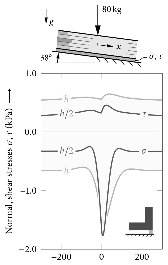
Figure 15Effect of changes of the slab thickness h on shear and normal stress in the weak layer under skier loading, shown for profile ![]() F.
F.
4.5 Example of extended analyses
As discussed in Sect. 2.4, the model covers complex cases with multiple external loads and several interacting cracks. An example is given in Fig. 18, where an inclined snowpack with profile ![]() B is loaded by two skiers in the vicinity of a weak-layer crack. For this analysis, five segments connected through transmission conditions were introduced to account for the discontinuities of two external loads and the crack. Figure 18a shows the obtained slab displacements and the rotations of slab cross sections. Both skiers locally increase deformations and interact, in particular with respect to deflections w0, owing to their proximity. The deformations of the layered slab above the crack of 100 cm length are even larger yet much smaller than the weak-layer thickness of 20 mm. Figure 18b shows the corresponding weak-layer shear and normal stresses. Again, the interaction of both loads, in particular in terms of normal stresses, is observed. Without load interaction, stresses would drop to the level of stresses induced by the slab weight alone in between the skiers. The effect is connected to bridging because the area across which individual loads are distributed depends on the snowpack's stiffness.
B is loaded by two skiers in the vicinity of a weak-layer crack. For this analysis, five segments connected through transmission conditions were introduced to account for the discontinuities of two external loads and the crack. Figure 18a shows the obtained slab displacements and the rotations of slab cross sections. Both skiers locally increase deformations and interact, in particular with respect to deflections w0, owing to their proximity. The deformations of the layered slab above the crack of 100 cm length are even larger yet much smaller than the weak-layer thickness of 20 mm. Figure 18b shows the corresponding weak-layer shear and normal stresses. Again, the interaction of both loads, in particular in terms of normal stresses, is observed. Without load interaction, stresses would drop to the level of stresses induced by the slab weight alone in between the skiers. The effect is connected to bridging because the area across which individual loads are distributed depends on the snowpack's stiffness.

Figure 16Bridging effect on the energy release rate in flat PST experiments. (a) Total differential energy release rate 𝒢 for profiles ![]() C,
C, ![]() D, and
D, and ![]() E. (b) Energy release rate 𝒢 normalized with respect to the square of the total slab weight ∑ρihi.
E. (b) Energy release rate 𝒢 normalized with respect to the square of the total slab weight ∑ρihi.
The proposed model uses the established concepts of laminate mechanics to assess the problem of layered slabs resting on weak layers. Heierli (2008) and Rosendahl and Weißgraeber (2020a) have shown that beam-type solutions can provide accurate representations of the mechanical response of homogeneous snowpacks loaded by gravity and localized loads. Analyses of layered snowpacks have only been performed with numerical models (Schweizer, 1993; Habermann et al., 2008) or with approximate solutions of limited generality (Monti et al., 2016). The validation in Sect. 3 shows that the present model provides an accurate closed-form analytical solution for layered slabs on a weak layer loaded by their own weight and external (point) loads. The comparison to the numerical reference solution demonstrates a high accuracy of the solution in terms of displacements, stresses, and also energy release rates of anticracks within the weak layer. The latter is obtained by using the analysis approaches developed for so-called weak interfaces exhibiting high elastic contrasts (Fraisse and Schmit, 1993; Lenci, 2001).
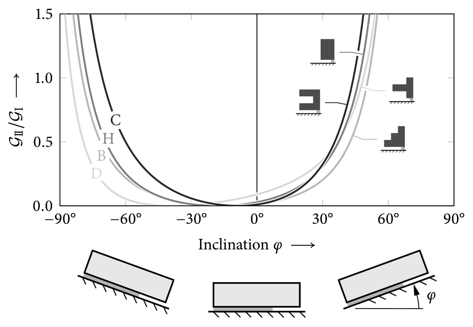
Figure 17Effect of slope angle on the mode mixity of the energy release rates in propagation saw tests. Mode mixity is expressed as the ratio of mode II (shear) to mode I (collapse) energy release rate (). PSTs are 2.5 m long and cut a=50 cm from the right.
The anisotropic mechanical response of the slab is described by the stiffnesses of laminate mechanics. The extensional stiffness A11 and the shear stiffness A55 are linear with respect to the thickness of the individual layers within the slab and do not depend on the ordering. The bending–extension coupling stiffness B11 is zero for symmetric laminates and scales both with the square of the individual layer thickness and linearly with z distance to the coordinate origin. Hence, it depends on the order of layers. This is even more pronounced for the bending stiffness D11 that depends on the power of three of the layer thicknesses and on the square of the distance to midplane. That is, both stiffnesses account for the complex mechanical behavior of a layered structure while accounting for layer ordering effects.
Table 3 shows that within the considered examples, decisive differences between the stiffnesses of different profiles can occur. The profile pairs ![]() A,
A, ![]() B and
B and ![]() E,
E, ![]() F each have the same extensional and bending stiffnesses, A11 and D11, respectively, and only the sign of the bending–extension stiffness B11 differs. Profiles
F each have the same extensional and bending stiffnesses, A11 and D11, respectively, and only the sign of the bending–extension stiffness B11 differs. Profiles ![]() C and
C and ![]() D exhibit a strong layering effect.
In the equivalent-layer concept (Monti et al., 2016), the layer moduli are homogenized into one equivalent Young modulus of the slab. To use models for homogeneous elastic half-spaces (e.g., Föhn, 1987), this system of slab and weak layer is then replaced with a single layer with the Young modulus of the weak layer and the slab thickness is scaled to account for this. Of course, such a homogenization works for extension deformation as well as bending deformation. However, Table 3 and Fig. 11 show that using this concept does not yield correct stiffness properties of the slab. As pointed out by Monti et al. (2016), the equivalence layer concept does not account for the order of the layers. Hence, the significant ordering effects of the considered profiles cannot be not accounted for.
It is worth noting that the equivalence layer concept also depends on the Young modulus of the weak layer.
D exhibit a strong layering effect.
In the equivalent-layer concept (Monti et al., 2016), the layer moduli are homogenized into one equivalent Young modulus of the slab. To use models for homogeneous elastic half-spaces (e.g., Föhn, 1987), this system of slab and weak layer is then replaced with a single layer with the Young modulus of the weak layer and the slab thickness is scaled to account for this. Of course, such a homogenization works for extension deformation as well as bending deformation. However, Table 3 and Fig. 11 show that using this concept does not yield correct stiffness properties of the slab. As pointed out by Monti et al. (2016), the equivalence layer concept does not account for the order of the layers. Hence, the significant ordering effects of the considered profiles cannot be not accounted for.
It is worth noting that the equivalence layer concept also depends on the Young modulus of the weak layer.
Birkeland et al. (2014) address the role of the slab on the crack propagation. They changed the slab by introducing cuts normal to the surface that significantly reduce the thickness locally. As shown in Fig. 16, when normalized for different profile weights, the reduced bending stiffness leads to much lower energy release rates that may not suffice for crack propagation. In a PST experiment, the weight of the slab is the only load and is constant along the weak layer. In a skier-loaded snowpack, the local loading of the skier leads to a locally increased energy release rate in the vicinity of the skier. With low bending stiffness, this energy release rate attains locally high values but then rapidly decreases to energy release rates originating from the slab's weight only. With higher bending stiffnesses, the influenced domain of a localized loading (e.g., a skier) is larger while the magnitude of the effect decreases.
The deformations of the slab (Fig. 12) show the resulting effect of the layering. This is pronounced as the longitudinal deformation at the interface of the slab and the weak layer depends strongly on the beam rotation ψ. That is, with increased bending stiffness of a slab, the longitudinal deformations at the weak layer will also be smaller, leading to reduced shear loading of the weak layer. The analysis of the stresses in the weak layer (Fig. 13) shows that the layering and the order of the layers control weak layer stresses and the effective bridging length (Schweizer and Camponovo, 2001a). In particular, the stress peaks below the localized loading of the skier will change with bridging. For stiffer slabs, a wider area below the skier is loaded while the maximum stresses decrease. Besides the stress loading in the weak layer, the energy released during crack initiation and growth controls avalanche release. The energy release rate, too, shows a pronounced effect of the stiffness of the slab and the ordering of the layers (Fig. 14). Slabs with high stiffness layers adjacent to the weak layer lead to higher energy release rates (in the considered PST configuration). The present results agree with the findings by Schweizer and Jamieson (2003), van Herwijnen and Jamieson (2007), and Thumlert and Jamieson (2014) that identified an increase in snowpack stability with increased bridging. Moreover, the results of the current model on the energy release rate of layered slabs can explain why failure propagation may be accentuated by stiff slabs, also reported by van Herwijnen and Jamieson (2007).
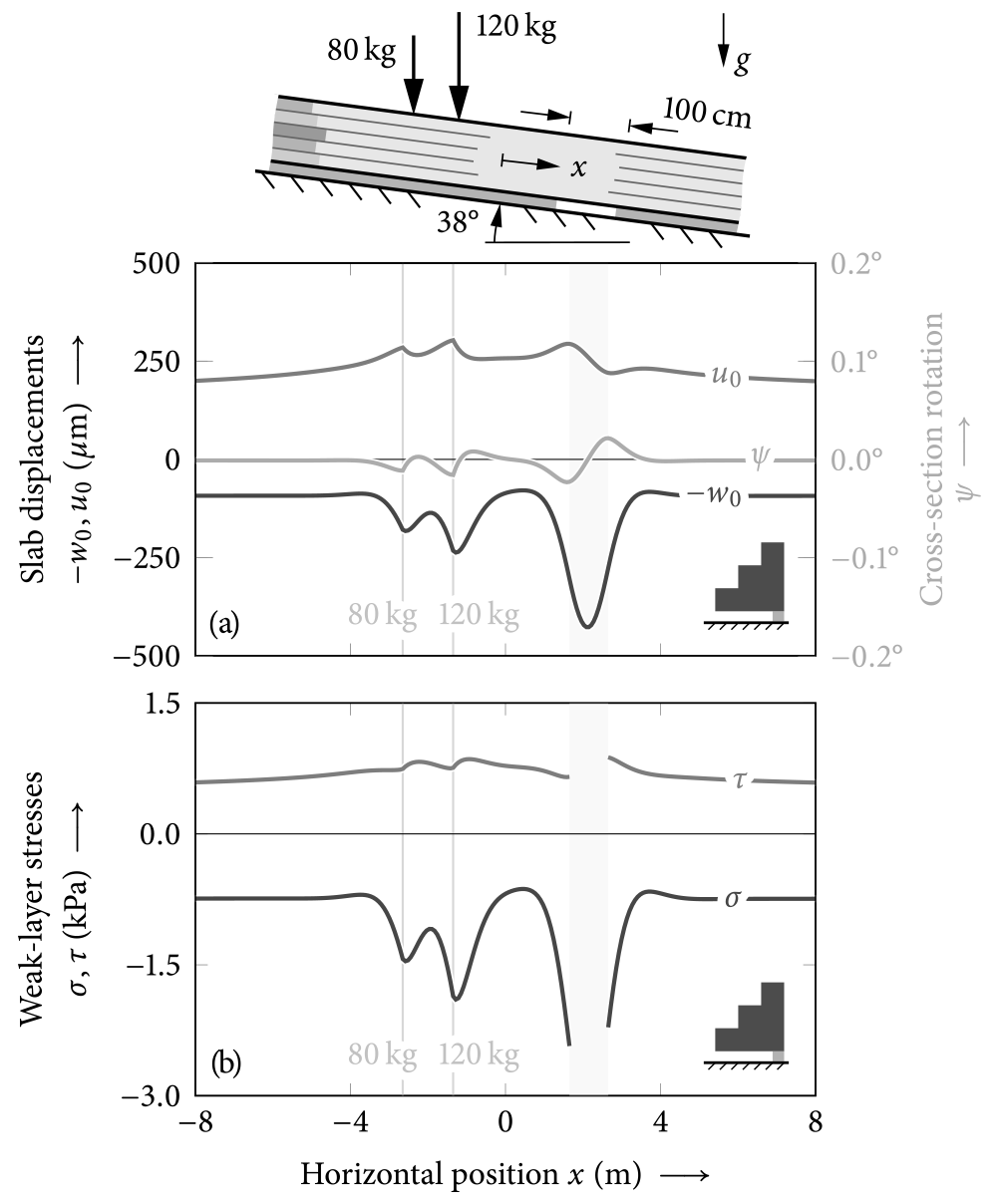
Figure 18Example of a complex configuration with two skier loads on profile ![]() B in the vicinity of a 100 cm weak-layer crack. Note that positive deflections w0 point in the physical downward direction. Here, we show −w0 to maintain the intuitive downward direction of a positive w0 when displayed on the same abscissa as u0.
B in the vicinity of a 100 cm weak-layer crack. Note that positive deflections w0 point in the physical downward direction. Here, we show −w0 to maintain the intuitive downward direction of a positive w0 when displayed on the same abscissa as u0.
In the studies by Schweizer and Jamieson (2003) and Thumlert and Jamieson (2014), a bridging index (BI) is introduced and applied to the analysis of snowpack stability. The bridging index accounts for the hand hardness index and the thickness of each layer. We propose to use the bending stiffness D11 to characterize the bridging of a snowpack configuration. Then, the ordering of the layers and the nonlinear contribution of the thickness to the bending behavior is considered. By restricting the consideration to this single property, effects such as shear deformation, bending–extension coupling, or weak layer deformation are not considered, but it will provide a good first indication of the bridging. For a full analysis, the use of a comprehensive and efficient model like the present one is advised.
The effect of the stiffness is also studied using profiles in which the layer order remains the same but each layer thickness is changed by the same factor (Fig. 15). With half the thickness of each layer, the total bending stiffness is reduced by a factor of 8. Hence, the bridging area is reduced, and the maximum peak stress increases, although the general stress level in the weak layer has decreased due to the lower total weight of the thinner layered slab. For energy release rates in PST experiments, weight loading dominates and heavier profiles (![]() C >
C > ![]() A >
A > ![]() F) feature higher energy release rates (Fig. 16a). Only when normalizing for the slab weight does an increased bending stiffness (
F) feature higher energy release rates (Fig. 16a). Only when normalizing for the slab weight does an increased bending stiffness (![]() C >
C > ![]() A >
A > ![]() F)
reduce the energy release (Fig. 16b).
F)
reduce the energy release (Fig. 16b).
Investigating the effect of the slope angle on energy release rates of PST experiments (Fig. 17) offers intriguing views of the behavior of PSTs and its experimental variants. The slab above the cut is subject to two sources of shear loading: (i) transverse shear deformation from the shear force of the weight of the overhanging slab and (ii) lateral shear loading of the tangential component qt of the gravitational load. On a flat slope, the latter vanishes. On inclines, its sign changes with negative and positive slope angles. The former has the same sign regardless of positive or negative inclination. Hence, shear contributions to the energy release rate are superimposed either additively or subtractively depending on the sign of the slope angle. Our results show that for upslope cuts, mode II plays a much smaller role than for downslope slope cuts. This has a direct effect on the mode II energy release rate and constitutes a significant difference between the two possible cut directions. Sigrist and Schweizer (2007), who were able to obtain relatively large contributions from shear deformations in their PST experiments, used downslope cuts. Whether this was done for the purpose of obtaining large mode II contributions or coincidence is not reported but is consistent with the present results. The findings may be used to develop PST procedures specifically designed to study mode I and mode II separately. Previously, some variations of PST experiments have been proposed in literature (e.g., Birkeland et al., 2019).
Even with increasing number of comprehensive numerical models, closed-form analytical models are highly relevant. As pointed out in the broad review by Morin et al. (2020), there is still a large need for an improved understanding of snow physics and for models that can assess snowpack stability. Especially for the use in model chains, extensive parametric studies, or in optimizations, a very high computational efficiency is very important. Within this work we have performed a total number of 6875 different analyses in the considered non-exhaustive parametric studies. This alone highlights the necessity of highly efficient, functional mechanical models. Moreover, in their simplistic structure, analytical models reveal fundamental physical interrelationships and effects. The present model in particular uses only input parameter with clear physical meaning that can be determined in relatively simple experiments. No numerical stabilization such as artificial viscosity or tuning parameters for complex constitutive laws that are not directly accessible in experiments are used or required.
The present model makes use of fundamental structural mechanisms and allows for insights into the mechanics of dry-snow slab avalanche release. The model can be used to implement failure models or to analyze experimental results. A similar model for homogeneous slabs (Rosendahl and Weißgraeber, 2020a) has been used by Bergfeld et al. (2021a) to identify the Young modulus of a slab by means of digital image correlation of PST experiments. The authors observed that the model provided consistent results for the Young modulus of the slab and weak layer, irrespective of experimentally recorded cut lengths. In contrast, using the expression of the system's elastic energy provided by Heierli et al. (2008), as proposed by van Herwijnen et al. (2016), showed a significant dependence on the cut length and led to inconsistent results. This can be attributed to the negligence of weak-layer elasticity by Heierli et al. (2008) and demonstrates the importance of considering the principal features of a physical problem. In the case of slab avalanche release, we view the mechanics of the layered slab and the weak layer as crucial.
For the proposed model, the computational effort does not change with domain size or number of considered layers. Computing the eigenvalues of the system matrix K of the governing ODE (11) represents the main computational effort. This is independent of the number of segments or layers, and it only needs to be done once for any set of boundary conditions, load cases, and slope angles. Each segment adds six free coefficients, i.e., 6 degrees of freedom to the linear system of equations of Eq. (18). This has virtually no impact on the computation effort even with 20 segments. In this case, timing 1000 stress evaluations yields a mean run time of 0.7 ms per analysis on a single 2.4 GHz Intel Core i9.
The model does not account for contact of the slab with base layers or the remains of a collapsed weak layer. For long weak-layer cracks, the corresponding normal deformations may become too large to be rendered correctly in the present model. A corresponding extension of the present model is a work in progress and will allow for the analysis of sustained anticrack growth. As discussed, the weak-interface concept used brings the limitation that cracks shorter than a few millimeters cannot be studied.
The present work presents a closed-form analytical model for the mechanical response of a layered slab resting on compliant weak layers.
-
It is applicable to slopes loaded by one or multiple skiers and propagation saw tests.
-
The model provides anisotropic slab stiffnesses, slab displacement fields, weak-layer stresses, and energy release rates of cracks in the weak layer that are in excellent agreement with finite-element reference solutions.
-
Its implementation is highly efficient, allows for real-time applications, and allows for the consideration of arbitrary system sizes and an arbitrary number of layers. It can be readily used to implement novel failure models.
-
In an analysis of bridging, we reveal significant effects of slab weight, stiffness, and layering on weak-layer stresses and energy release rates.
-
Based on an investigation of inclined propagation saw tests, we recommend upslope cut PSTs for the analyses for mode I energy release rates and downslope cut PSTs for mode II analyses.
With the first derivative of the constitutive equation of the normal force Eq. (7a)′ inserted into the equilibrium of horizontal forces Eq. (6a), we obtain
Likewise, with the first derivative of the constitutive equation of the shear force Eq. (7b)′ and the vertical force equilibrium Eq. (6b), we have
The first derivative of the constitutive equation of the bending moment Eq. (7a)′ with the balance of moments Eq. (6c) yields
We then insert the definition of the shear stresses Eq. (5b) into Eq. (A1) to obtain
Inserting the normal stress definition Eq. (5a) into Eq. (A2) yields
and, again, inserting the shear stress (5b) into Eq. (A3) yields
Equations (A4) to (A6) constitute a system of linear ordinary differential equations of second order with constant coefficients of the deformation variables that describes the mechanical behavior of a layered beam on a weak layer.
Using the vector z(x) of all unknown functions (10), the ODE system can be written as a system of first order for the form
with the matrices
and
where
and the vector
The system (A7) can be rearranged into the form
where
Without an elastic foundation, the equilibrium conditions (6a) and (6b) reduce to
By adding and subtracting to the constitutive equation of the bending moment (Eq. 7a) and using the first derivative of the constitutive equation of the shear force (Eq. 7b)′, we obtain
Differentiating twice and using the first derivatives of the equilibrium conditions, Eqs. (B2)′ and (B3)′ yield
Adding and subtracting to the constitutive equation of the normal force (Eq. 7a) and using the constitutive equation of the shear force (Eq. 7b) gives
Differentiating this equation and, again, using the derivatives of the equilibrium conditions, Eqs. (B1)′ and (B2)′ yield
Solving the derivative of this equation for and inserting it into Eq. (B5) yields an ordinary differential equation of fourth order for the vertical displacement:
It can be solved readily by direct integration:
Solving Eq. (B7) for , integrating twice, and inserting the third derivative of the general solution for w0(x) (Eq. B9)′ yields the general solution for the tangential displacement of unsupported beams:
To obtain a solution of the cross-section rotation ψ(x), we take the derivative of the constitutive equation for the bending moment (Eq. 7a)′ and insert it together with the constitutive equation of the shear force (Eq. 7b) into the equilibrium of moments (Eq. B3). Solving this for ψ(x) yields
Equation (B7) allows for eliminating . In order to eliminate ψ′′(x), we insert the constitutive equation of the shear force (Eq. 7b) into the second derivative of the vertical equilibrium (Eq. B2)′′, which yields , and we obtain
which is fully defined through the solution for w0(x) (Eq. B9).
In order to assemble a global system of linear equations from boundary and transmission conditions between supported and unsupported beam segments, it is helpful to express the general solutions for both cases in the same form. For this purpose, we express vector of unknown functions (Eq. 10) used for the solution of supported beam segments through the general solutions Eqs. (B12) to (B9) for unsupported beam segments. This yields the matrix form (see Eq. 16), where is the vector of unknown coefficients,
and
with .
Stability tests are typically conducted on finite volumes with free ends that require vanishing section forces and moments,
as boundary conditions. Skier-induced loading is typically confined in a very small volume compared to the overall dimensions of the snowpack that extends over the entire slope. For the model, this corresponds to an unbounded domain, where all components of the solution converge to a constant at infinity. That is, at the boundaries, the complementary solution vector must vanish:
which yields constant displacements z(x)=zp; see Eq. (13).
At interfaces between two segments (e.g., change from supported to unsupported), 𝒞0 continuity of displacements and section forces is required and the transmission conditions read
where the Δ operator indicates the difference between left and right segments, i.e., .
External concentrated forces (e.g., skiers) are introduced as discontinuities of the section forces. They are considered with their normal and tangential components Fn and Ft and with their resulting moment . They have to be accounted for in the form of the transmission conditions between two segments:
where, again, the Δ operator expresses the difference between left and right segments. Therefore, at points of such loads the slab must always be split into segments to allow for the definition of the transmission conditions.
The in-plane stresses σx, σz, and τxz within layers of the slab are obtained using the layers' constitutive equations and exploiting the equilibrium conditions (Reddy, 2003). Using Hooke's law and the identities , the axial layer normal stresses can be expressed in terms of slab displacements in the form
where Young's modulus E(z) and Poisson's ratio ν(z) are layerwise, i.e., piecewise, constant in the z direction. Integrating the local equilibrium condition
with respect to z, where derivatives with respect to y vanish owing to the plane-strain assumption, yields the in-plane layer shear stress
The second-order derivatives are obtained from the left-hand side of Eq. (11), and integration with respect to z is performed using the trapezoidal rule. Again, integrating the equilibrium condition
with respect to z under the same assumptions, yields the interlayer normal stresses
Here, differentiation is performed using difference quotients with consideration of discontinuities. Finally, maximum (σI) and minimum (σIII) principal stresses are computed from
A Python implementation of the present model is publicly available at https://github.com/2phi/weac (last access: 28 March 2023), Zenodo (https://doi.org/10.5281/zenodo.5810763, Rosendahl and Weißgraeber, 2022), and https://pypi.org/project/weac (Rosendahl and Weißgraeber, 2023).
Data used in this work were generated using the software resources cited in the “Code availability” section and can be reproduced using the input data given herein. Additional data used for model validation were taken from the literature. Finite-element model outputs are available upon request.
PW and PLR contributed equally to the design and implementation of the model, to the analysis of the results, and to the writing of the manuscript.
The contact author has declared that neither of the authors has any competing interests.
Publisher's note: Copernicus Publications remains neutral with regard to jurisdictional claims in published maps and institutional affiliations.
We acknowledge support by the German Research Foundation and the Open Access Publishing Fund of the Technical University of Darmstadt. We are grateful for the support by Florian Rheinschmidt, who provided the finite-element reference model.
This research has been supported by the German Research Foundation and the Open Access Publishing Fund of the Technical University of Darmstadt to cover open-access article processing charges.
This paper was edited by Guillaume Chambon and reviewed by three anonymous referees.
Bair, E. H.: Forecasting artificially-triggered avalanches in storm snow at a large ski area, Cold Reg. Sci. Technol., 85, 261–269, https://doi.org/10.1016/j.coldregions.2012.10.003, 2013. a
Bergfeld, B., van Herwijnen, A., Reuter, B., Bobillier, G., Dual, J., and Schweizer, J.: Dynamic crack propagation in weak snowpack layers: insights from high-resolution, high-speed photography, The Cryosphere, 15, 3539–3553, https://doi.org/10.5194/tc-15-3539-2021, 2021a. a
Bergfeld, B., van Herwijnen, A., Reuter, B., Bobillier, G., Dual, J., and Schweizer, J.: Dynamic crack propagation in weak snowpack layers: Insights from high-resolution, high-speed photography, The Cryosphere Discuss. [preprint], https://doi.org/10.5194/tc-2020-360, 2021b. a, b
Bergfeld, B., van Herwijnen, A., Bobillier, G., Rosendahl, P. L., Weißgraeber, P., Adam, V., Dual, J., and Schweizer, J.: Temporal evolution of crack propagation characteristics in a weak snowpack layer: conditions of crack arrest and sustained propagation, Nat. Hazards Earth Syst. Sci., 23, 293–315, https://doi.org/10.5194/nhess-23-293-2023, 2023a. a, b, c, d
Bergfeld, B., van Herwijnen, A., and Schweizer, J.: Time series data on dynamic crack propagation in long propagation saw tests, EnviDat [data set], https://doi.org/10.16904/envidat.365, 2023b. a, b, c
Birkeland, K., van Herwijnen, A., Knoff, E., Staples, M., Bair, E., and Simenhois, R.: The role of slabs and weak layers in fracture arrest, in: Proceedings ISSW, 156–168, http://arc.lib.montana.edu/snow-science/item/2045 (last access: 29 March 2023), 2014. a, b
Birkeland, K. W., van Herwijnen, A., Reuter, B., and Bergfeld, B.: Temporal changes in the mechanical properties of snow related to crack propagation after loading, Cold Reg. Sci. Technol., 159, 142–152, https://doi.org/10.1016/j.coldregions.2018.11.007, 2019. a
Bobillier, G., Gaume, J., van Herwijnen, A., Dual, J., and Schweizer, J.: Modeling the propagation saw test with discrete elements, in: Proceedings of the International Snow Science Workshop ISSW 2018, edited by: Fischer, J.-T., Adams, M., Dobesberger, P., Fromm, R., Gobiet, A., Granig, M., Mitterer, C., Nairz, P., Tollinger, C., and Walcher, M., Innsbruck, Austria, 976–980, http://arc.lib.montana.edu/snow-science/item/2690 (last access: 29 March 2023), 2018. a
Broberg, K. B.: The near-tip field at high crack velocities, International J. Fract., 39, 1–13, https://doi.org/10.1007/BF00047435, 1989. a, b
Camponovo, C. and Schweizer, J.: Measurements on skier triggering, in: Proceedings of the International Snow Science Workshop 1996, 100–103, http://arc.lib.montana.edu/snow-science/item/1415 (last access: 29 March 2023), 1997. a
De Barros, S. T.: Deflection factor charts for two-and three-layer elastic systems, Highway Research Record, 145, 83–108, http://onlinepubs.trb.org/Onlinepubs/hrr/1966/145/145-005.pdf (last access: 29 March 2023), 1966. a
Fletcher, R. C. and Pollard, D. D.: Anticrack model for pressure solution surfaces, Geology, 9, 419–424, 1981. a, b
Föhn, P. M. B.: The stability index and various triggering mechanisms, in: Avalanche Formation, Movement and Effects (Proceedings of the Davos Symposium, Sept. 1986), IAHS Publ., 195–214, 1987. a, b, c, d
Föhn, P. M. B.: Simulation of surface-hoar layers for snow-cover models, Ann. Glaciol., 32, 19–26, https://doi.org/10.3189/172756401781819490, 2001. a
Fraisse, P. and Schmit, F.: Use of J-integral as fracture parameter in simplified analysis of bonded joints, Int. J. Fract., 63, 59–73, 1993. a
Gaume, J. and Reuter, B.: Assessing snow instability in skier-triggered snow slab avalanches by combining failure initiation and crack propagation, Cold Reg. Sci. Technol., 144, 6–15, https://doi.org/10.1016/j.coldregions.2017.05.011, 2017. a, b
Gaume, J., van Herwijnen, A., Chambon, G., Birkeland, K. W., and Schweizer, J.: Modeling of crack propagation in weak snowpack layers using the discrete element method, The Cryosphere, 9, 1915–1932, https://doi.org/10.5194/tc-9-1915-2015, 2015. a
Gaume, J., van Herwijnen, A., Chambon, G., Wever, N., and Schweizer, J.: Snow fracture in relation to slab avalanche release: critical state for the onset of crack propagation, The Cryosphere, 11, 217–228, https://doi.org/10.5194/tc-11-217-2017, 2017. a
Gaume, J., Gast, T., Teran, J., van Herwijnen, A., and Jiang, C.: Dynamic anticrack propagation in snow, Nat. Commun., 9, 3047, https://doi.org/10.1038/s41467-018-05181-w, 2018. a
Gauthier, D. and Jamieson, B.: Evaluation of a prototype field test for fracture and failure propagation propensity in weak snowpack layers, Cold Reg. Sci. Technol., 51, 87–97, https://doi.org/10.1016/j.coldregions.2007.04.005, 2008. a
Gauthier, D. and Jamieson, B.: On the Sustainability and Arrest of Weak Layer Fracture in Whumpfs and Avalanches, in: Proceedings of the International Snow Science Workshop, vol. 1, 224–231, http://arc.lib.montana.edu/snow-science/item/376 (last access: 29 March 2023), 2010. a, b
Geldsetzer, T. and Jamieson, B.: Estimating dry snow density from grain form and hand hardness, in: International Snow Science Workshop, 121–127, https://arc.lib.montana.edu/snow-science/item/717 (last access: 29 March 2023), 2000. a
Gerling, B., Löwe, H., and van Herwijnen, A.: Measuring the Elastic Modulus of Snow, Geophys. Res. Lett., 44, 11088–11096, https://doi.org/10.1002/2017GL075110, 2017. a
Goland, M. and Reissner, E.: The stresses in cemented joints, J. Appl. Mech., 11, A17–A27, 1944. a
Habermann, M., Schweizer, J., and Jamieson, B.: Influence of snowpack layering on human-triggered snow slab avalanche release, Cold Reg. Sci. Technol., 54, 176–182, https://doi.org/10.1016/j.coldregions.2008.05.003, 2008. a, b, c, d, e, f
Heierli, J.: Anticrack model for slab avalanche release, PhD thesis, Universität Karlsruhe, https://doi.org/10.5445/IR/1000011033, 2008. a
Heierli, J. and Zaiser, M.: An analytical model for fracture nucleation in collapsible stratifications, Geophys. Res. Lett., 33, L06501, https://doi.org/10.1029/2005GL025311, 2006. a
Heierli, J. and Zaiser, M.: Failure initiation in snow stratifications containing weak layers: Nucleation of whumpfs and slab avalanches, Cold Reg. Sci. Technol., 52, 385–400, https://doi.org/10.1016/j.coldregions.2007.02.007, 2008. a
Heierli, J., Gumbsch, P., and Zaiser, M.: Anticrack nucleation as triggering mechanism for snow slab avalanches, Science, 321, 240–243, https://doi.org/10.1126/science.1153948, 2008. a, b, c, d, e
Huang, Y. H.: Slope Stability Analysis by the Limit Equilibrium, American Society of Civil Engineers, ISBN 978-0-7844-1288-6, 2014. a
Hübsch, J. D., Rosendahl, P. L., and Mittelstedt, C.: An analytical failure model for pressurized blister tests of thermally loaded composite laminates, Compos. Part B-Eng., 214, 108588, https://doi.org/10.1016/j.compositesb.2020.108588, 2021. a
Jamieson, B. and Schweizer, J.: Texture and strength changes of buried surface-hoar layers with implications for dry snow-slab avalanche release, J. Glaciol., 46, 151–160, https://doi.org/10.3189/172756500781833278, 2000. a
Jamieson, J. and Johnston, C.: Refinements to the stability index for skier-triggered dry-slab avalanches, Ann. Glaciol., 26, 296–302, 1998. a
Jones, R. M.: Mechanics of composite materials, 2nd Edn., CRC press, ISBN 9781315272986, https://doi.org/10.1201/9781498711067, 1998. a
Klarmann, R. and Schweizerhof, K.: A Priori Verbesserung von Schubkorrekturfaktoren zur Berechnung von geschichteten anisotropen Schalentragwerken, Arch. Appl. Mech., 63, 73–85, https://doi.org/10.1007/BF00788914, 1993. a
Krenk, S.: Energy release rate of symmetric adhesive joints, Eng. Fract. Mech., 43, 549–559, https://doi.org/10.1016/0013-7944(92)90198-N, 1992. a, b
Leguillon, D.: Strength or toughness? A criterion for crack onset at a notch, Eur. J. Mech. A-Solid., 21, 61–72, https://doi.org/10.1016/S0997-7538(01)01184-6, 2002. a
Lehning, M., Fierz, C., Brown, B., and Jamieson, B.: Modeling snow instability with the snow-cover model SNOWPACK, Ann. Glaciol., 38, 331–338, 2004. a
Lenci, S.: Analysis of a crack at a weak interface, Int. J. Fract., 108, 275–290, 2001. a, b, c
McClung, D.: Fracture energy applicable to dry snow slab avalanche release, Geophys. Res. Lett., 34, L02503, https://doi.org/10.1029/2006GL028238, 2007. a
McClung, D. and Schweizer, J.: Fracture toughness of dry snow slab avalanches from field measurements, J. Geophys. Res.-Earth, 111, F04008, https://doi.org/10.1029/2005JF000403, 2006. a
McClung, D. M.: Shear Fracture Precipated by Strain Softening as a Mechanism of Dry Slab Avalanche Release, J. Geophys. Res., 84, 3519–3526, 1979. a
McClung, D. M.: Fracture mechanical models of dry slab avalanche release, J. Geophys. Res.-Sol. Ea., 86, 10783–10790, https://doi.org/10.1029/JB086iB11p10783, 1981. a
McClung, D. M. and Schweizer, J.: Skier triggering, snow temperatures and the stability index for dry-slab avalanche initiation, J. Glaciol., 45, 190–200, https://doi.org/10.3189/002214399793377121, 1999. a
Monti, F., Gaume, J., van Herwijnen, A., and Schweizer, J.: Snow instability evaluation: calculating the skier-induced stress in a multi-layered snowpack, Nat. Hazards Earth Syst. Sci., 16, 775–788, https://doi.org/10.5194/nhess-16-775-2016, 2016. a, b, c, d, e, f, g, h, i, j, k
Morin, S., Horton, S., Techel, F., Bavay, M., Coléou, C., Fierz, C., Gobiet, A., Hagenmuller, P., Lafaysse, M., Ližar, M., Matjaž Ližar, Mitterer, C., Monti, F., Müller, K., Olefs, M., Snook, J. S., van Herwijnen, A., and Vionnet, V.: Application of physical snowpack models in support of operational avalanche hazard forecasting: A status report on current implementations and prospects for the future, Cold Reg. Sci. Technol., 170, 102910, https://doi.org/10.1016/j.coldregions.2019.102910, 2020. a, b
Neuber, H.: Theorie der technischen Formzahl, Forschung auf dem Gebiete des Ingenieurwesens, 7, 271–274, https://doi.org/10.1007/BF02584908, 1936. a
Peterson, R. E.: Methods of correlating data from fatigue tests of stress concentration specimens, in: Stephen Timoshenko Anniversary Volume, Macmillan, New York, 179–183, 1938. a
Reddy, J. N.: Mechanics of Laminated Composite Plates and Shells: Theory and Analysis, 2nd Edn., CRC Press, Boca Raton, https://doi.org/10.1201/b12409, 2003. a, b, c
Reiweger, I., Gaume, J., and Schweizer, J.: A new mixed-mode failure criterion for weak snowpack layers, Geophys. Res. Lett., 42, 1427–1432, https://doi.org/10.1002/2014GL062780, 2015. a
Reuter, B., Schweizer, J., and van Herwijnen, A.: A process-based approach to estimate point snow instability, The Cryosphere, 9, 837–847, https://doi.org/10.5194/tc-9-837-2015, 2015. a
Richter, B., van Herwijnen, A., Rotach, M. W., and Schweizer, J.: Sensitivity of modeled snow stability data to meteorological input uncertainty, Nat. Hazards Earth Syst. Sci., 20, 2873–2888, https://doi.org/10.5194/nhess-20-2873-2020, 2020. a
Rosendahl, P. L. and Weißgraeber, P.: Modeling snow slab avalanches caused by weak-layer failure – Part 1: Slabs on compliant and collapsible weak layers, The Cryosphere, 14, 115–130, https://doi.org/10.5194/tc-14-115-2020, 2020a. a, b, c, d, e
Rosendahl, P. L. and Weißgraeber, P.: Modeling snow slab avalanches caused by weak-layer failure – Part 2: Coupled mixed-mode criterion for skier-triggered anticracks, The Cryosphere, 14, 131–145, https://doi.org/10.5194/tc-14-131-2020, 2020b. a, b, c, d
Rosendahl, P. L. and Weißgraeber, P.: Weak Layer Anticrack Nucleation Model (WEAC), Zenodo [code], https://doi.org/10.5281/zenodo.5810763, 2022. a, b
Rosendahl, P. L. and Weißgraeber, P.: Weak Layer Anticrack Nucleation Model, https://pypi.org/project/weac/, last access: 28 March 2023. a
Rosendahl, P. L., Staudt, Y., Schneider, A. P., Schneider, J., and Becker, W.: Nonlinear elastic finite fracture mechanics: Modeling mixed-mode crack nucleation in structural glazing silicone sealants, Materials Design, 182, 108057, https://doi.org/10.1016/j.matdes.2019.108057, 2019. a
Schweizer, J.: The influence of the layered character of snow cover on the triggering of slab avalanches, Ann. Glaciol., 18, 193–198, https://doi.org/10.3189/S0260305500011496, 1993. a, b
Schweizer, J. and Camponovo, C.: The skier's zone of influence in triggering slab avalanches, Ann. Glaciol., 32, 314–320, https://doi.org/10.3189/172756401781819300, 2001a. a
Schweizer, J. and Camponovo, C.: The skier’s zone of influence in triggering slab avalanches, Ann. Glaciol., 32, 314–320, 2001b. a
Schweizer, J. and Jamieson, J. B.: Snowpack properties for snow profile analysis, Cold Reg. Sci. Technol., 37, 233–241, 2003. a, b, c
Schweizer, J. and Jamieson, J. B.: A threshold sum approach to stability evaluation of manual snow profiles, Cold Reg. Sci. Technol., 47, 50–59, 2007. a
Schweizer, J. and Wiesinger, T.: Snow profile interpretation for stability evaluation, Cold Reg. Sci. Technol., 33, 179–188, 2001. a
Schweizer, J., Schneebeli, M., Fierz, C., and Föhn, P. M.: Snow mechanics and avalanche formation: Field experiments on the dynamic response of the snow cover, Surv. Geophys., 16, 621–633, 1995. a
Sigrist, C.: Measurement of fracture mechanical properties of snow and application to dry snow slab avalanche release, PhD thesis, ETH Zürich, https://doi.org/10.3929/ethz-a-005282374, 2006. a
Sigrist, C. and Schweizer, J.: Critical energy release rates of weak snowpack layers determined in field experiments, Geophys. Res. Lett., 34, L03502, https://doi.org/10.1029/2006GL028576, 2007. a, b, c
Sih, G. C.: Strain-energy-density factor applied to mixed mode crack problems, Int. J. Fract., 10, 305–321, https://doi.org/10.1007/BF00035493, 1974. a
Smith, F. and Curtis, J.: Stress analysis and failure prediction in avalanche snowpacks, IAHS Publication, 114, 332–340, 1975. a
Smith, T. L. and Chu, W. H.: Ultimate tensile properties of elastomers. VII. Effect of crosslink density on time–temperature dependence, J. Polym. Sci. A2, 10, 133–150, https://doi.org/10.1002/pol.1972.160100110, 1972. a
Stein, N., Weißgraeber, P., and Becker, W.: A model for brittle failure in adhesive lap joints of arbitrary joint configuration, Compos. Struct., 133, 707–718, 2015. a
Thumlert, S. and Jamieson, B.: Stress measurements in the snow cover below localized dynamic loads, Cold Reg. Sci. Technol., 106-107, 28–35, https://doi.org/10.1016/j.coldregions.2014.06.002, 2014. a, b, c
van Herwijnen, A. and Jamieson, B.: Snowpack properties associated with fracture initiation and propagation resulting in skier-triggered dry snow slab avalanches, Cold Reg. Sci.Technol., 50, 13–22, https://doi.org/10.1016/j.coldregions.2007.02.004, 2007. a, b, c, d
van Herwijnen, A., Gaume, J., Bair, E. H., Reuter, B., Birkeland, K. W., and Schweizer, J.: Estimating the effective elastic modulus and specific fracture energy of snowpack layers from field experiments, J. Glaciol., 62, 997–1007, https://doi.org/10.1017/jog.2016.90, 2016. a, b, c
Waddoups, M. E., Eisenmann, J. R., and Kaminski, B. E.: Macroscopic Fracture Mechanics of Advanced Composite Materials, J. Compos. Mater., 5, 446–454, https://doi.org/10.1177/002199837100500402, 1971. a
Weißgraeber, P., Felger, J., Geipel, D., and Becker, W.: Cracks at elliptical holes: Stress intensity factor and Finite Fracture Mechanics solution, Eur. J. Mech. A-Solid., 55, 192–198, https://doi.org/10.1016/j.euromechsol.2015.09.002, 2015. a
Weighted by the moment of area of the cross section of zeroth, first, and second order.
- Abstract
- Introduction
- Mechanical model
- Model validation
- Results
- Discussion
- Conclusions
- Appendix A: Derivation of the governing equations for a layered slab supported by an elastic foundation
- Appendix B: Derivation of the governing equations of an unsupported layered slab
- Appendix C: Boundary and transmission conditions
- Appendix D: Slab stress fields
- Code availability
- Data availability
- Author contributions
- Competing interests
- Disclaimer
- Acknowledgements
- Financial support
- Review statement
- References