the Creative Commons Attribution 4.0 License.
the Creative Commons Attribution 4.0 License.
 | 15 Mar 2023
Brief communication: Monitoring active layer dynamics using a lightweight nimble ground-penetrating radar system – a laboratory analogue test case
Emmanuel Léger
Albane Saintenoy
Mohammed Serhir
François Costard
Christophe Grenier
Monitoring active layer dynamics is critical for improving the understanding of near-surface thermal and hydrological processes in the cryosphere. This study presents the laboratory test of a low-cost ground-penetrating radar (GPR) system within a laboratory experiment of active layer freezing and thawing monitoring. The system is an in-house-built low-power monostatic GPR antenna coupled with a reflectometer piloted by a single-board computer (SBC) and was tested prior to field deployment. The correspondence between the frozen front electromagnetic (EM) reflection and temperature allowed us to test the ability of the system to closely monitor the frozen front and bottom of the active layer reflection.
- Article
(2773 KB) - Full-text XML
-
Supplement
(33679 KB) - BibTeX
- EndNote


The freezing and thawing cycles of frozen material in the cryosphere environment are not only important processes for water and temperature redistributions but also critical for nutrient cycles (nitrogen and carbon) and atmospheric gas release. As such, the non-destructive monitoring of the seasonal soil freezing and thawing in high-latitudinal contexts has been an extensive topic of interest in cold regions. Previous researchers have illustrated the suitability of geophysical methods, especially ground-penetrating radar (GPR) techniques, for monitoring active layer freezing and thawing (Liu and Arcone, 2003; van der Kruk et al., 2009; Jadoon et al., 2015; van der Kruk et al., 2007; Westermann et al., 2010; Steelman and Endres, 2009; Sudakova et al., 2021). Reflections from the permafrost table, or active layer base, were compared in GPR profiles with acquisitions repeated at different times (Westermann et al., 2010; Sudakova et al., 2021). The first 10 cm cycle of soil freezing and thawing over 9 d was monitored using a static antenna set of an air-launched off-ground GPR system (Jadoon et al., 2015). With the same steady monitoring approach, common mid-point techniques were used to study electromagnetic (EM) wave dispersion and frequency to infer active layer freezing and thawing acting as waveguide (van der Kruk et al., 2009; Steelman and Endres, 2009). As far as we know, no studies were performed using a monostatic on-ground antenna that monitors the same location through time, apart from a first attempt in the laboratory with a commercial antenna system (Saintenoy et al., 2005). Here, we present a novel combination of low-cost and low-energy nimble GPR monostatic ground antenna coupled with a reflectometer in conjunction with a small array of thermal and volumetric water content sensors for monitoring active layer freezing and thawing during laboratory experiments. The study is considered a first test case on an active layer laboratory analogue before near-future field deployments.
2.1 Autonomous monitoring ground-penetrating radar system (M-GPR)
The monitoring ground-penetrating radar system (M-GPR) system comprises an ultra-wide band antenna, designed in the GeePs Laboratory, operating in frequency band 0.1–6 GHz. The antenna is a fractal-folded complementary bow-tie antenna (Liu et al., 2018). It is combined with the R60 Copper Mountain (http://coppermountaintech.com, last access: 9 March 2023) vector network analyser to measure the reflection coefficient (in this case S11) of the antenna placed in front of the area under test (Fig. 1). The antenna design has been engineered with fractals in order to enlarge the covered bandwidth. It is enclosed in a shielded cavity to reduce backward radiation and to protect it from external electromagnetic (EM) perturbations. Inside the cavity, absorbers are placed to prevent the antenna performance degradation while reducing multiple reflections.

Figure 1Experimental setup: (a) draft of the experiment where volumetric water content sensors are on the left and thermistors on the right side of the draft; the cryogenic fluid is flowing at the bottom of the tank at −10 ∘C. (b) This picture depicts the GPR prototype with the (2) antenna and (3) reflectometer in the cold room. (c) This picture shows the four main components of the M-GPR system: (1) UDOO SBC computer, (2) butterfly antenna, (3) reflectometer and (4) power-supply timer plugged into a 12 V car battery. The pencil gives the scale.
The R60 Copper Mountain reflectometer is controlled (via serial USB connection) using an UDOO single-board computer (SBC; SECO S.P.A.). The board is powered using a stabilised current source (12 V) and a timer (CRONTAB) to allow power and sleep modes for long time monitoring campaign. For the presented results, a stack of 10 traces was performed regularly in time (every 5 min) where the real and imaginary part of S11 were recorded over 801 points covering the frequency band 0.2–5 GHz. The frequency-domain measurement data were inverse Fourier transformed to generate time-domain radargrams with a time window of 30 ns. The expected dynamic range of measured data can reach up to 90 dB using the R60 Copper Mountain reflectometer and adopting the step-frequency technique. In addition, on a 12 V, 60 Ah battery, the GPR system offers the possibility to monitor during a month with a measurement every 5 min, including the pre-heating of the reflectometer and a stack of 10 traces. Using the M-GPR system, one can configure the timer to wake-up the UDOO SBC every 12 h in order to monitor the area under investigation during months.
2.2 Laboratory modelled active layer characteristics
The laboratory analogue active layer was made of Fontainebleau fine sand (D50=200 µm) contained in a cylindrical vase-shaped reservoir of 52 cm height and 84–90 cm diameter, as drafted and shown in Fig. 1a and b. At the base of the column, a system of homemade copper pipes was installed and connected to an external cryostat-flowing glycol in the copper pipes at −10 ∘C. The freezing copper pipes were surrounded by a gravel layer, used as drainage horizon and spreading the weight of the above sand layer. A thin layer of aluminium foil with multiple holes was placed above the gravel layer to create a strong bottom reflector. A thin geotextile sheet was set on top of the drainage–freezing layer for preventing the sand being flushed out and to minimise frost heave according to Henry (1990). The inner diameter of the cylinder was covered by polystyrene foam blankets all around its inner diameter, to ensure radial thermal insulation as much as possible and keep only the top (atmosphere +1 ∘C) and bottom (copper pipe linked to cryostat) boundaries (−10 ∘C) as open thermal flow conditions.
The cylindrical tank was hydraulically connected to tap water with a buffer reservoir system allowing us to set the water table at different heights. This system allowed us to properly and incrementally saturate the sand material while compacting it in the reservoir. The sand hydrodynamic parameters, such as the parameters by Mualem (1976) and van Genuchten (1980) can be found in Léger et al. (2020). A well-proven technique (Costard et al., 2021) was used to create a homogeneous porous medium of more than 400 kg of saturated soil: we manually compacted layers of 10 cm each by maintaining the water level higher than the considered layer and then putting them on top of each other until 0.47 m thickness was reached. The sand was packed to a porosity estimated to be 0.39. There might be some small interfaces (thin unconformities), but they remain insignificant (as was verified post-experimentally when excavating the sand).
The low-temperature external atmospheric conditions were set using the cold room facility at the GEOPS laboratory (University Paris Saclay, France) dedicated to the physical modelling in periglacial geomorphology (Costard et al., 2021). The external temperature of the cold room was maintained slightly above +1 ∘C, throughout the freezing phase. For shortening the thawing time length, the thawing phase was performed by shutting down all freezing processes, opening the cold room and equilibrating with ambient temperature in the building (≈ +20 ∘C). As shown in Fig. 1a), a string of 10 thermistors (PT100 with ±0.1 ∘C) were set from the bottom of the sand layer to the surface at 0, 2.5, 5, 7.5, 10, 15, 20, 30, 40 and 47 cm from the bottom. Complementing these thermal measurements, three volumetric water content sensors (Meter Terros 12, https://metergroup.com, last access: 9 March 2023) were set diametrically opposed to the thermistor string at 10, 20 and 30 cm from the bottom of the sand layer. In addition to the sensor network, a handheld thermal camera (Flir TG297, Teledyne FLIR LLC) was used to check the thermal isolation continuity of the cylindrical reservoir, notably the thermal insulating polystyrene layer on the curvilinear sides of the reservoir.
2.3 Electromagnetic wave velocity as a function of soil dielectric properties
The monostatic antenna emits and receives frequency sweep of spherical electromagnetic (EM) waves in response to the reflectometer excitation at different frequencies. The receiving antenna converts the incoming EM fields to electrical digital signals. Following the work of Annan (1999), the velocity of an EM wave that propagates in non-magnetic soil, with low electrical conductivity, can be approximated by
where ε′ denotes the real part of the relative dielectric permittivity and c=0.3 m ns−1 is the velocity of EM waves in air.
The dielectric permittivity depends on the media component content, such as water, air, minerals and ice content. We used the volumetric mean complex refractive index model (Birchak et al., 1974), where the relative dielectric permittivity of the porous material, εb, is a function of the material porosity, its state of saturation and the respective permittivity of each of its individual constituents. For the thawed water-saturated case, assuming no air is entrapped, the Fontainebleau sand medium is biphasic, composed of water and silica:
where εw and εs are respectively the relative dielectric permittivity of water and of silica, ϕ is the porosity and γ is an empirical coefficient that depends on soil structure. In this study, we set εw=80.1, εs=4.2, ϕ=0.39 and γ=0.5 as in Léger et al. (2020). We assumed all media were non-conductive and no dispersion effect was taken into account. The frozen case was similar to Eq. (2), except that the liquid water phase was replaced by its solid phase, considering that no air was entrapped and that no change in porosity was resulting from the freezing phase,
where εi is the relative dielectric permittivity of ice (set here to 3.1). A transitional zone was assumed between these two types of media (frozen and unfrozen) where coexistence between frozen and thawed media was derived using an empirical freezing curve (the sinus of the ice content percentage in pores decreasing linearly from 100 to 0) without considering any change in porosity through the freezing process. This modelling, despite its simplicity, is thought of as a first numerical analogue to the media aiming to roughly simulate a bottom freezing active layer.
2.4 Electromagnetic modelling
For simulating our M-GPR data, we used the open-source software GprMax2D (Warren et al., 2016), in two dimensions, as presented in Léger et al. (2020). The EM model was set to 1.2 m wide and 0.6 m high, larger than the real model to avoid side effects, filled up to 0.47 m with saturated sand following the simplistic permittivity distribution presented in Sect. 2.3. The cell size was 5×5 mm2. A perfect electrical conductor (PEC) layer was set at the bottom of the sand layer and the model domain sides were padded with 10-cell-thick absorbing boundaries. The freezing layer was modelled using the dielectric permittivity distribution (derived from Eq. 3), corresponding to a frozen layer increasing from 0.02 m up to 0.3 m with 2 cm step. The GPR antenna was modelled by a Hertzian dipole polarised in the direction perpendicular to the two-dimensional plane model, emitting a Ricker waveform centred on 1.5 GHz. This simplistic EM model was considered as a first try aiming to understand where the various reflections originated from during the bottom active layer freezing.
While a total of eight experiments have been carried out, due to sand quantity involved and the time to freeze and thaw, we present in detail the results of one experiment; four others are available in the Supplement.
3.1 Temperature and volumetric liquid water content time series
The temperature time series measured during one of the experiments are presented in Fig. 2a. During the equilibrating phase, the surface temperature sensor drops the fastest to the constant cold room temperature (+1 ∘C). The thermal time series exhibit little 8 h cycles for the shallowest sensor at the surface due to the chamber cryostat defrost cycles, maintaining the cold room at +1 ∘C. The bottom freezing phase start is marked by the dashed blue vertical line at 21:00 CET on day 21 corresponding to the zero experimental time. At the base of the sand layer, the temperature reaches the 0 ∘C isotherm within a few hours with a typical curtain effect for the sensors close to the cold system (z=0, 2.5, 5 cm), while almost a day is required for sensors from 20 cm to the top. Near-surface and surface sensors (40 cm and Surface) are within the 0 ∘C isotherm. Once the 0 ∘C isotherm is crossed, the temperatures follow an exponential decrease as expected (Hinzman et al., 1998). The depth–temperature profile derived from the time series presented in Fig. 2c exhibits the depth of the 0 ∘C isotherm reaching the ground surface after 60 h from the start of the experiment. Once the freezing phase is done, the thawing phase exhibits a fast thawing for the first 30 cm below the surface, while it takes more time deeper, with an optimum at 10 cm corresponding to the balance between heat dissipation and proximity to the bottom freezing cold source inertia. The heat dissipation is also visible on the different evolutions of the curve with depth.
The volumetric liquid water content in the column is homogeneous during the equilibrating phase, Fig. 2b, except the 20 cm sensor is slightly lower compared to the rest of the column, probably due to a miscalibration or water-unsaturated macropore(s) nearby. During the freezing phase, a little bump is observed right before dropping because of water freezing. This bump gets wider as the sensor height is increasing, corresponding to liquid water pushed up by the frozen front. The 30 cm sensor is the last to be frozen and the first to be thawed.
Soil-freezing characteristic curves (SFCs) at different depths were determined from volumetric water content and temperature data collected during the experiment (Fig. 2d). Neither a supercooling effect as those observed in more complex soils (Ren and Vanapalli, 2020) nor a strong zero-curtain effect was observed. Hysteresis in the SFCs are observed for each depth due to air and/or water and/or ice entrapment.
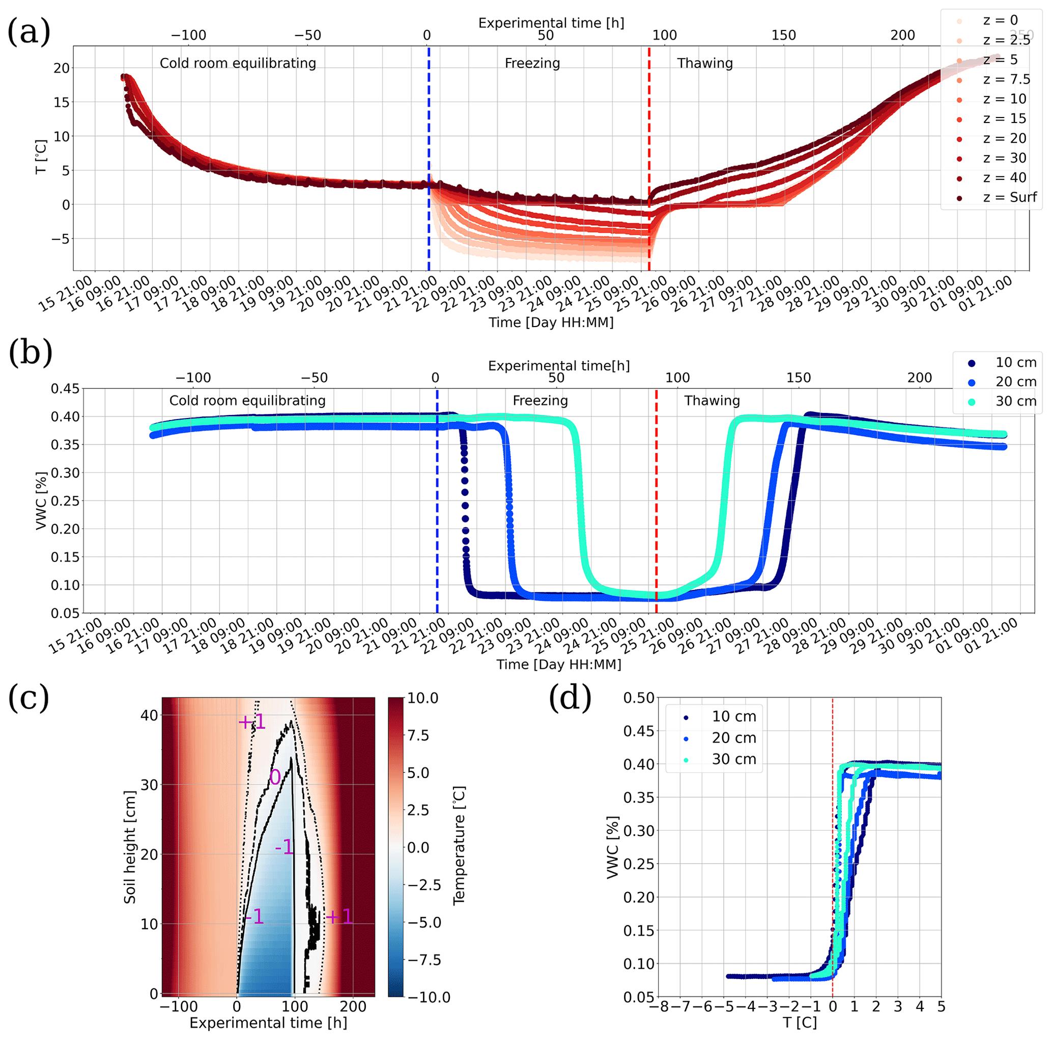
Figure 2Temperature and volumetric water content monitoring of the experiment: (a) thermal monitoring, (b) volumetric water content monitoring, (c) reconstructed two-dimensional temperature column, (d) soil-freezing curves. Depth of the sensors are in centimetres from the base of the sand layer. Dashed blue line represents the start of the freezing phase, while the dashed red line represents the end of the freezing phase and the beginning of thawing.
3.2 Monitoring ground-penetrating radar system (M-GPR)
The simulated radargram is presented in Fig. 3a. To recap, each trace has been computed from a dielectric permittivity distribution (derived from Eqs. 2 and 3) corresponding to a frozen layer that is increased from 0.02 m up to 0.3 m with 2 cm step. They are presented in Fig. 3b. The two-way travel time (TWT) of the reflection on the PEC layer (labelled A), represented as yellow crosses in Fig. 3a, has been computed from each permittivity distribution in the tank. Two reflections (B) and (C) arrive earlier than reflection (A), directly linked to the frozen–thawed water saturated sand transition as seen in Fig. 3b, where (A) is placed at the bottom of the tank and points (B) and (C) are placed on sharp permittivity contrasts. We use this simple modelling to interpret the experimental radargram.
The experimental M-GPR radargram, presented in Fig. 3c, displays three main reflections; these are labelled (A), (B) and (C). Comparing the experimental radargram to the simulated one, we find visual correspondences strengthening our assumption: the first (C) reflection corresponds to the frost table, while the (B) reflection corresponds to the bottom of the transitional zone and the (A) reflection to the aluminium PEC sheet. As opposed to the numerical case, (B) and (C) reflections are difficult to discriminate during the freezing phase but easier to distinguish during the thawing phase. The dynamic used in the numerical modelling (keeping a fixed transitional zone thickness) does not fit the experimental data (where the transitional thickness is clearly increasing with experimental time in Fig. 2c). Beyond the reflection similarity, the amplitude and wavelet are different, mostly due to the different EM sources, the loss not taken into account in the modelling, the homogeneity and the isotropy, which are present in the experimental radargram.
These (B) and (C) reflections give us information about the thickness, the homogeneity and the dynamics of the active layer during the freezing and thawing phases. We especially detect the speed of thawing being faster than the speed of freezing and water redistribution in the near surface. In addition, subtracting the TWTs of these reflections (TWTA-TWTC) and comparing them with the 0 ∘C isotherm height inferred from the thermistor time series (Fig. 2a and c), gives the time needed for the electromagnetic wave to propagate through the frozen media as a function of its thickness. Figure 2d shows that the points (TWTs as a function of frozen front height) align in a linear relationship, inversely proportional to the squared root of the bulk permittivity. By adjusting the linear regression with Theil–Sen robust regression at 90 % confidence interval, we retrieve a bulk permittivity at , similar to the literature for saturated frozen sand (Arcone et al., 1998).
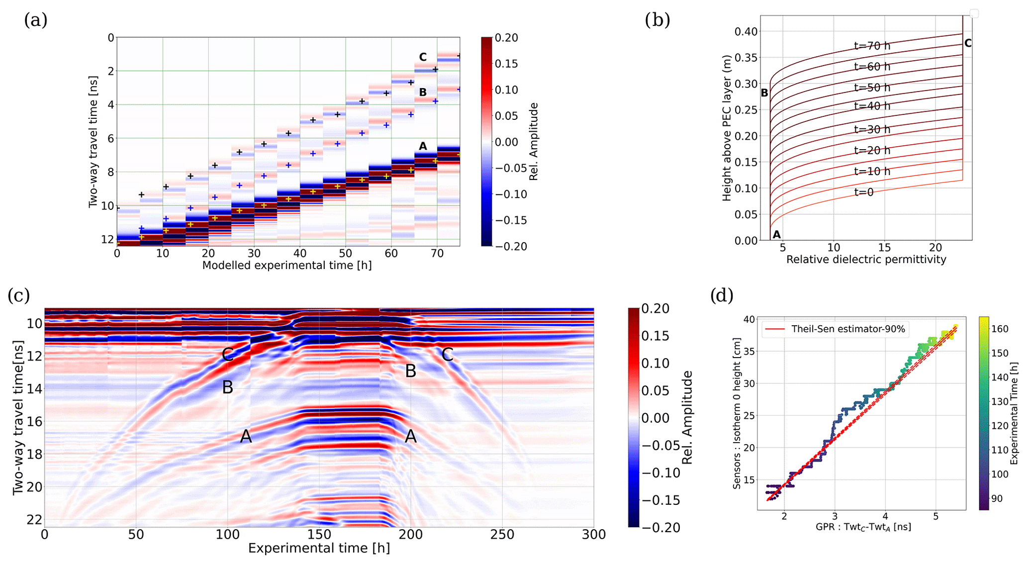
Figure 3(a) Simulated radargram with permittivity distributions shown in (b). (c) Experimental radargram displayed with normalised amplitude. Labelled (A), (B) and (C) reflections correspond to the permafrost base, bottom and top of the transitional zone, respectively. Crosses in (a) are computed as TWT using permittivity distributions in (b), where B and C positions are indicated for the t=65 h. TWT stands for Two-Way travel Time. (d) The difference of TWTC and TWTA as a function of 0 ∘C-isotherm height.
The M-GPR system has proved to be capable of delivering the evolution of the thaw depth and the average soil water content between the surface and the freeze–thaw interface for the freezing and thawing periods. For the laboratory conditions encountered in the study, the M-GPR method was able to monitor a moving interface with an uncertainty being less than a centimetre, being sufficient to secure spatial differences in the very small thaw depth dynamic. The modelling presented in this study is very simple but was aimed at understanding where the reflections observed in the experimental radargram were coming from. A coupled thermo–hydro–EM modelling is currently in development in order to fully simulate the physical phenomena and use the M-GPR data to infer SFCs.
In terms of technical drawbacks, the main factors limiting the accuracy in the present study are: (1) the frost heave through the experiment and (2) the surface condition changing the antenna impedance. The latter could be accounted for by using a bistatic antenna, allowing us to retrieve the near surface hydric conditions and thus the impedance of the antenna. The first issue regarding the frost heave is easy to track in a laboratory experiment: here, only 1–2 cm heave were observed since we used geotextiles, while it is harder in the case of field studies. Beyond frost heave, soil tilting and surface deplanarisation can happen and lead to loss of verticality and miscalculation of the depth of the frost table.
Due to its agility, the M-GPR system will be of use for better understanding the GPR reflection in the case of supra-permafrost water layer, especially if the reflection is due to the unsaturated soil–saturated soil interface and/or the freezing interface. The difficulty in interpreting the origin of reflections is illustrated by the difference in the modelling and the experimental radargram. As presented, the M-GPR system, is fully autonomous and can monitor during 2 months at 30 min intervals with a 12 V, 60 Ah car battery without any recharge. The field deployment is about to start, having been delayed due to international tensions. That being said, coupled with a set of temperature and volumetric water content, the method holds a strong potential for bringing valuable thermo–hydro–dynamical information and refines the various processes taking place during melting and freezing.
For GPR modelling we used gprmax, which can be found at https://github.com/gprMax/gprMax (last access: 9 March 2023) and Zenodo (https://doi.org/10.5281/zenodo.7727092, Léger, 2023). All the codes we used here were developed in Python and are available from the corresponding authors upon reasonable request.
All datasets are available from the corresponding author upon reasonable request.
The supplement related to this article is available online at: https://doi.org/10.5194/tc-17-1271-2023-supplement.
All authors participated in the conceptualisation. EL, AS and CG performed the experiments. EL and AS performed data curation. EL and AS did the formal analysis. AS, MS and FC brought experimental resources. AS and CG performed the funding acquisition. EL and AS wrote the original draft and conducted the reviews and editing.
The contact author has declared that none of the authors has any competing interests.
Publisher's note: Copernicus Publications remains neutral with regard to jurisdictional claims in published maps and institutional affiliations.
This study has been funded by the in situ extreme conditions instrumentation – AAP 2020 MITI SUPERLEVELING project INSU.
Critical reviews by Adam Booth and two anonymous reviewers greatly enhanced the presentation and the content of
this paper.
This article is dedicated to Christophe Grenier.
This research has been supported by the Institut national des sciences de l'Univers (In situ extreme conditions instrumentation grant).
This paper was edited by Adam Booth and reviewed by two anonymous referees.
Annan, A.: Ground Penetrating Radar: Workshop Notes, Tech. rep., Sensors and Software Inc., Ontario, Canada, 1999. a
Arcone, S. A., Lawson, D. E., Delaney, A. J., Strasser, J. C., and Strasser, J. D.: Ground-penetrating radar reflection profiling of groundwater and bedrock in an area of discontinuous permafrost, Geophysics, 63, 1573–1584, 1998. a
Birchak, J., Gardner, L., Hipp, J., and Victor, J.: High dielectric constant microwave probes for sensing soil moisture, Proc. IEEE, 35, 85–94, 1974. a
Costard, F., Dupeyrat, L., Séjourné, A., Bouchard, F., Fedorov, A., and Saint-Bézar, B.: Retrogressive Thaw Slumps on Ice-Rich Permafrost Under Degradation: Results From a Large-Scale Laboratory Simulation, Geophys. Res. Lett., 48, e2020GL091070, https://doi.org/10.1029/2020GL091070, 2021. a, b
Henry, K. S.: Laboratory investigation of the use of geotextiles to mitigate frost heave, Tech. rep., Cold regions research and engineering laboratory, Hanover, NH, https://apps.dtic.mil/sti/citations/ADA227335 (last access: 9 March 2023), 1990. a
Hinzman, L. D., Goering, D. J., and Kane, D. L.: A distributed thermal model for calculating soil temperature profiles and depth of thaw in permafrost regions, J. Geophys. Res.-Atmos., 103, 28975–28991, 1998. a
Jadoon, K. Z., Weihermüller, L., McCabe, M. F., Moghadas, D., Vereecken, H., and Lambot, S.: Temporal monitoring of the soil freeze-thaw cycles over a snow-covered surface by using air-launched ground-penetrating radar, Remote Sens., 7, 12041–12056, 2015. a, b
Léger, E.: Brief Communication: Monitoring active layer dynamic using a lightweight nimble Ground-Penetrating Radar system. A laboratory analog test case, Zenodo [data set], https://doi.org/10.5281/zenodo.7727092, 2023. a
Léger, E., Saintenoy, A., Coquet, Y., Tucholka, P., and Zeyen, H.: Evaluating hydrodynamic parameters accounting for water retention hysteresis in a large sand column using surface GPR, J. Appl. Geophys., 182, 104176, https://doi.org/10.1016/j.jappgeo.2020.104176, 2020. a, b, c
Liu, L. and Arcone, S. A.: Numerical simulation of the wave-guide effect of the near-surface thin layer on radar wave propagation, J. Environ. Eng. Geoph., 8, 133–141, 2003. a
Liu, X., Serhir, M., and Lambert, M.: Detectability of junctions of underground electrical cables with a ground penetrating radar: Electromagnetic simulation and experimental measurements, Constr. Build. Mater., 158, 1099–1110, 2018. a
Mualem, Y.: A new model for predicting the hydraulic conductivity of unsaturated porous media, Water Resour. Res., 12, 513–522, 1976. a
Ren, J. and Vanapalli, S. K.: Effect of freeze–thaw cycling on the soil-freezing characteristic curve of five Canadian soils, Vadose Zone J., 19, e20039, https://doi.org/10.1002/vzj2.20039, 2020. a
Saintenoy, A., Tucholka, P., Bailleul, J., Costard, F., Elie, F., and Labbeye, M.: Modeling and monitoring permafrost thawing in a controlled laboratory experiment, in: Proceedings of the 3rd International Workshop on Advanced Ground Penetrating Radar, 79–83, https://doi.org/10.1109/AGPR.2005.1487855, 2005. a
Steelman, C. M. and Endres, A. L.: Evolution of high-frequency ground-penetrating radar direct ground wave propagation during thin frozen soil layer development, Cold Reg. Sci. Technol., 57, 116–122, 2009. a, b
Sudakova, M., Sadurtdinov, M., Skvortsov, A., Tsarev, A., Malkova, G., Molokitina, N., and Romanovsky, V.: Using ground penetrating radar for permafrost monitoring from 2015–2017 at calm sites in the Pechora river delta, Remote Sensing, 13, 3271, https://doi.org/10.3390/rs13163271, 2021. a, b
van der Kruk, J., Arcone, S. A., and Liu, L.: Fundamental and higher mode inversion of dispersed GPR waves propagating in an ice layer, IEEE T. Geosci. Remote S., 45, 2483–2491, 2007. a
van der Kruk, J., Steelman, C., Endres, A., and Vereecken, H.: Dispersion inversion of electromagnetic pulse propagation within freezing and thawing soil waveguides, Geophys. Res. Lett., 36, L18503, https://doi.org/10.1029/2009GL039581, 2009. a, b
van Genuchten, M. T.: A Closed form equation for predicting the hydraulic conductivity of unsaturated soils, Soil Sci. Soc. Am. J., 44, 892–898, 1980. a
Warren, C., Giannopoulos, A., and Giannakis, I.: gprMax: Open source software to simulate electromagnetic wave propagation for Ground Penetrating Radar, Comput. Phys. Commun., 209, 163–170, 2016. a
Westermann, S., Wollschläger, U., and Boike, J.: Monitoring of active layer dynamics at a permafrost site on Svalbard using multi-channel ground-penetrating radar, The Cryosphere, 4, 475–487, https://doi.org/10.5194/tc-4-475-2010, 2010. a, b