A sensor-agnostic albedo retrieval method for realistic sea ice surfaces: model and validation

A framework was established for remote sensing of sea ice albedo that integrates sea ice physics with high computational efficiency and that can be applied to optical sensors that measure appropriate radiance data. A scientific machine learning (SciML) approach was developed and trained on a large synthetic dataset (SD) constructed using a coupled atmosphere–surface radiative transfer model (RTM). The resulting RTM–SciML framework combines the RTM with a multi-layer artificial neural network SciML model. In contrast to the Moderate Resolution Imaging Spectroradiometer (MODIS) MCD43 albedo product, this framework does not depend on observations from multiple days and can be applied to single angular observations obtained under clear-sky conditions. Compared to the existing melt pond detection (MPD)-based approach for albedo retrieval, the RTM–SciML framework has the advantage of being applicable to a wide variety of cryosphere surfaces, both heterogeneous and homogeneous. Excellent agreement was found between the RTM–SciML albedo retrieval results and measurements collected from airplane campaigns. Assessment against pyranometer data (N=4144) yields RMSE = 0.094 for the shortwave albedo retrieval, while evaluation against albedometer data (N=1225) yields RMSE = 0.069, 0.143, and 0.085 for the broadband albedo in the visible, near-infrared, and shortwave spectral ranges, respectively.

1 Introduction

Sea ice regulates global climate through several feedback mechanisms.¹ Broadband albedo is a critical parameter determining the radiative energy balance of the complex atmosphere–cryosphere system.

For decades, optical sensors deployed on geostationary and polar-orbiting satellites have been used to derive the global-scale surface broadband albedo. However, the majority of albedo products are land-surface products, while ocean surface albedo data (including sea ice) are left blank (Qu et al., 2015). Table 1 compares the currently operational products and algorithms capable of retrieving albedo at the sea ice surface.

Key et al. (2016)Riihelä et al. (2013); Karlsson et al. (2017)Kharbouche and Muller (2018)Lucht et al. (2000); Schaaf et al. (2002)Zege et al. (2015); Istomina et al. (2015)Istomina (2020)Qu et al. (2016)Peng et al. (2018)

Table 1 Summary of the currently operational products and algorithms capable of retrieving albedo at the cryosphere's surface.

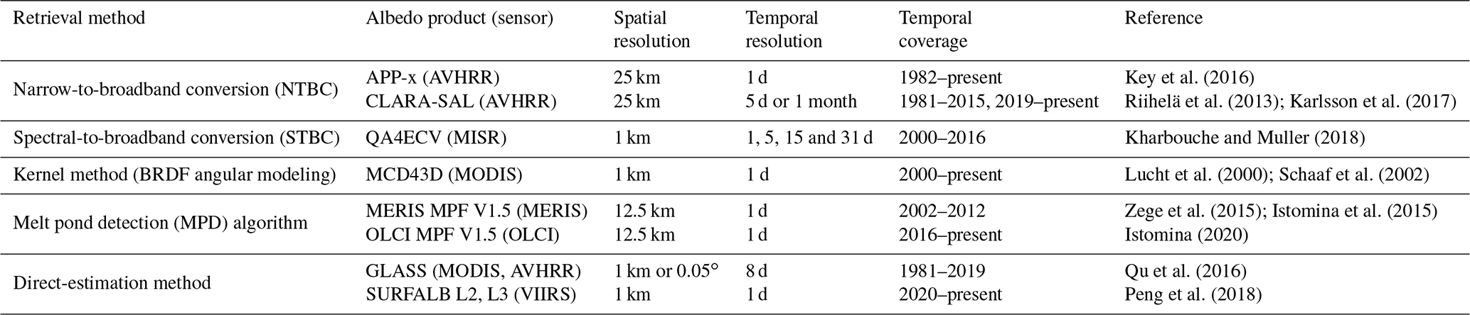
The broadband albedo estimated by APP-x is based on a narrow-to-broadband conversion (NTBC) of reflectance under a Lambertian surface assumption (Key et al., 2016), which implies that the radiance reflected from the surface is isotropic and that the value of albedo equals π times the reflected radiance. However, fresh snow and white ice surfaces cannot be considered Lambertian; dry snow and ice surfaces exhibit strong forward scattering, and the impact of the bidirectional distribution of radiance reflected must be rectified in a post-processing step as discussed by Li et al. (2007).

Taking into account the anisotropic properties of the sea ice surface, the (broadband) albedo retrieval procedure requires three steps: (1) atmospheric correction, (2) anisotropy correction to obtain narrow-band or spectral albedo, and (3) use of spectral to broadband conversion (STBC) to integrate over the spectral range to obtain (or alternatively derive coefficients to estimate) broadband albedo (Knap et al., 1999; Liang, 2000; Xiong et al., 2002; Stroeve et al., 2005). The STBC coefficients derived by Liang et al. (1999); Liang (2000) were applied to retrieve sea ice albedo using Medium Resolution Imaging Spectrometer (MERIS) and Multi-angle Imaging SpectroRadiometer (MISR) instruments, respectively (Gao et al., 2004; Kharbouche and Muller, 2018). The retrievals are based on atmospherically corrected level 2 (reflectance) data from the instruments, as opposed to level 1 (radiance) data measured at the top of the atmosphere (TOA).

The Moderate Resolution Imaging Spectroradiometer (MODIS) MCD43A and MCD43D products describe the effect of reflectance anisotropy on land–ocean surfaces using the RossThick-LiSparse (RTLSR) model provided by Lucht et al. (2000), which is a semi-empirical linear kernel-driven model that requires a sufficient amount of cloud-free observations within a 16 d window. Because MCD43 is a land albedo product, it only delivers very limited shortwave albedo values near the coast due to the lack of a spectral bi-directional reflectance distribution function (BRDF) for sea ice surfaces. In fact, there are only a few BRDF measurements that can be used to assist in correcting the anisotropy of snow and sea ice surfaces (e.g., Gatebe et al., 2005; Dumont et al., 2010; Gatebe and King, 2016), and they are far from conclusive in covering the complicated sea ice surface or encompassing a sufficient angular and spectral range.

Due to the scarcity of observations, in more recent efforts the BRDF of the cryosphere surface is approximated using radiative transfer models (RTMs). Examples of such efforts are the sea ice albedo retrieval based on the melt pond detection (MPD) algorithm (Zege et al., 2015) and the direct-estimation algorithm (Qu et al., 2016). Both algorithms try to establish a relation between TOA-measured radiance and surface albedo in two steps; the radiative processes in the atmosphere and on the cryosphere surface were considered independently (i.e., “uncoupled”). The atmospheric reflectance and transmittance are calculated with RTMs (Tynes et al., 2001; Vermote et al., 1997). Following this step, the calculated values are used to determine the TOA radiance and reflectance that corresponds to some specific surface condition, and the surface is modeled as the “linear blend” of sea ice, snow, melt pond, and water components.

In contrast, we present a framework that integrates a coupled atmosphere–surface RTM (Stamnes et al., 2018) with scientific machine learning (SciML) models. The coupled RTM model considers all radiative processes occurring in the coupled atmosphere, snow, and ice system. Multiple reflections between the surface and the atmosphere and the atmospheric molecular and aerosol-induced modifications to the incident spectral distribution of the solar radiation are both taken into account. At the atmosphere–surface interface, Fresnel's equations and Snells' law appropriately describe light interactions as required. Additionally, this RTM is combined with a snow, ice, and water model that simulates the snow and ice crystals and their inherent optical properties (IOPs); the snow, ice, and melt pond layering; and the impurities included within the snow, ice, and water layers (Stamnes et al., 2011).

In the direct-estimation method, the same IOPs were deployed to derive the BRDFs of the snow surface (Qu et al., 2016). However, because the direct-estimation algorithm decouples the atmosphere from the ocean layer, it is unable to accurately simulate the “snow-covered sea ice” situation; the “snow surface” scenario refers to snow that has been placed on land. In a coupled RTM, snow is correctly simulated as a layer of snow on the surface above the air–sea ice interface. Similarly, the MPD algorithm uses an uncoupled RTM. Based on the absorption of yellow pigments in ice, it models sea ice's BRDF exclusively for dry and white ice, ignoring the effects of air bubbles and brine pockets (Zege et al., 2015). In a coupled RTM, sea ice is simulated as a layer of ice with brine pockets and air bubble inclusions floating on deep ocean water.

This paper is structured as follows. Section 2 provides a summary of the RTM–SciML framework for albedo retrieval, describes the cloud screening and surface classification model, and introduces the validation and comparison datasets used in this study. Section 3 is devoted to validation of the albedo-retrieval products, and Sect. 4 addresses the possible sources of uncertainty in the validation data. In Sect. 5, the albedo product is compared to the MCD43 product (Sect. 5.1), two MPD-based products (MERIS and OLCI in Sects. 5.2 and 5.3, respectively) and two direct-estimation products (GLASS and VIIRS, in Sect. 5.4). A conclusion and summary are provided in Sect. 6.

2 Methodology

2.1 Overall framework

In this work, we present a new method for albedo retrieval: scientific machine learning based on a coupled RTM (hereafter RTM–SciML albedo algorithm). Figure 1 shows a flowchart of the proposed RTM–SciML framework for albedo retrieval, while Sect. 2.2–2.6 discuss the steps in more detail.

Figure 1 Flowchart of the proposed RTM–SciML framework for albedo retrieval.

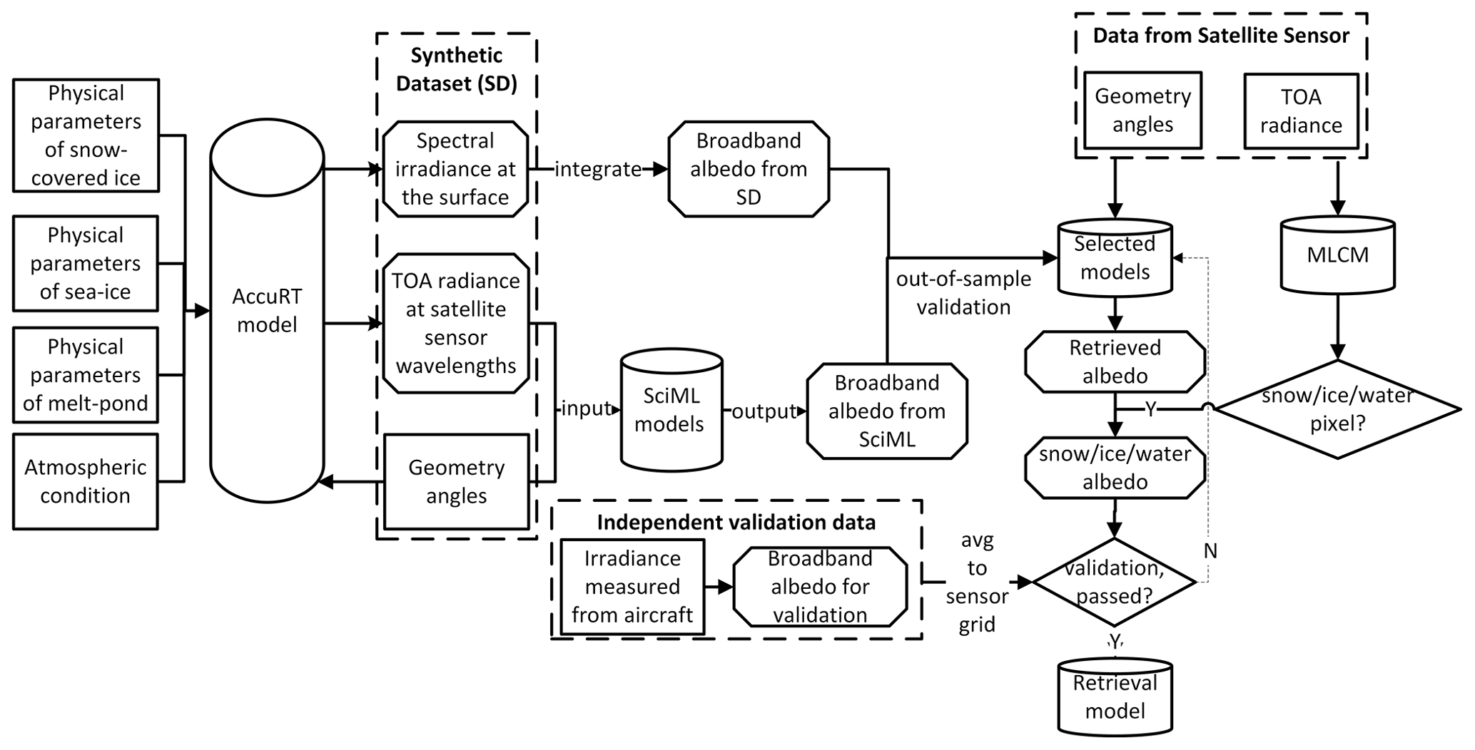
First, a synthetic dataset (SD) is constructed using a coupled-RTM, AccuRT (Stamnes et al., 2018). It consists of TOA radiances simulated in suitable satellite channels as a function of observational and solar angles, as well as the associated broadband albedo at the surface. This SD encompasses a range of different surface types, including snow-covered ice, melt ponds, and bare sea ice, as well as their mixtures. All optical properties of surface and atmospheric constituents, as well as radiative processes within the coupled atmosphere–snow–sea ice–water system, are deduced from first principles; information about both the surface BRDF and the IOPs of the atmosphere is implicitly taken into account. We are thus saved from the procedure of performing atmospheric corrections.

The coupled RTM ensures that the “forward problem” is solved correctly, yielding reliable total radiance and irradiance values at any location of the coupled system given the IOPs of the system constituents. Following the physically consistent SD, scientific machine learning (SciML) models can be used to approximate solutions to the “inverse problem”, which answers the following question through an implicit iterative process (i.e., by minimizing a loss function repeatedly during the training of SciML models): “given the observed TOA radiance and the sun–satellite geometry angles, what is the most likely albedo of the sea ice surface?” The SciML models perform without reliance on predefined spectral reflectance threshold values for individual types of surface, which eliminates errors caused by incorrect surface condition assumptions. When deployed in practice, the surface classification and albedo retrieval are separate processes; an independent machine learning classification mask (MLCM, described briefly in Sect. 2.4) performs both cloud screening and surface pixel classification.

2.2 Synthetic dataset (SD) generated by coupled RTM

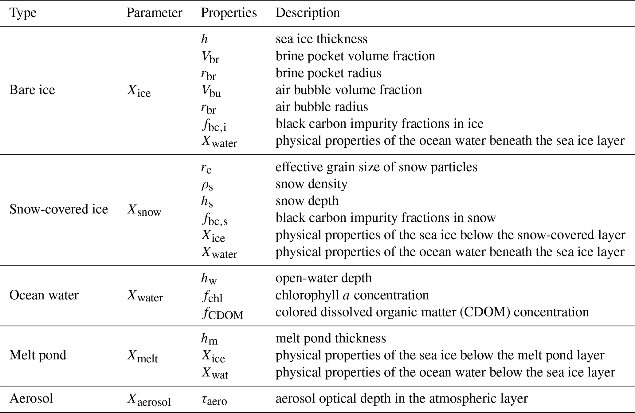
The AccuRT radiative transfer model (Stamnes et al., 2018) is able to simulate a coupled system with changes in refractive index across the atmosphere–water (in solid or liquid form) interface. Inputs to AccuRT are the IOPs of the two adjacent coupled slabs (upper slab is atmosphere and snow and lower slab is ocean and ice). Each slab can be partitioned into many adjacent layers, with the IOPs being constant within each layer but varying between them. The IOPs depend on the medium's absorption and scattering coefficients, as well as the scattering phase functions. Within the AccuRT computer code, Mie theory and the particle size distributions are used to generate IOPs based on user-defined physical properties of the medium (Stamnes et al., 2011). Table 2 summarizes the parameters used to calculate the IOPs of bare ice, snow-covered ice, open water, melt ponds, and aerosols. Appendix A discusses the value ranges of the physical parameters in more detail.

Among the sea ice inclusions, air bubbles are modeled as pure scatterers, brine pockets scatter and absorb light, and black carbon impurities mainly absorb light. The effective grain size r_e of snow particles closely resembles the effective light path traveled by a photon, and hence a larger r_e suggests a lower reflectance (and albedo). Additionally, bulk properties such as ice, pond, and snow thickness (h, h_m, h_s, respectively) and snow density (ρ_s) also impact the optical depth of the medium. Notably, the parameterizations employed here are consistent with the physics of sea ice, snow, and water (Grenfell and Maykut, 1977; Grenfell and Perovich, 1984; Warren, 2019).

Table 2 Properties used to compute the inherent optical properties (IOPs) of bare ice, snow-covered ice, open water, melt pond, and aerosol, which are utilized as inputs to the radiative transfer model (Stamnes et al., 2011).

Pseudo-random values of the physical parameters of ice, water, and snow within realistic ranges were applied to generate 158 000 cases each for (i) bare ice, (ii) ice with meltwater, and (iii) ice with snow cover (the value ranges are shown in Tables A1–A3). These surface and atmospheric parameters, together with randomly distributed solar and viewing geometries (Table A4) form a dataset suitable for generating a SD of TOA radiances and corresponding albedo values that can be used to train a SciML algorithm.

Altogether, the 158 000 × 3=474 000 configurations cover most expected combinations of surface types and atmospheric conditions encountered during the sea ice life cycle. For each case, TOA radiances at appropriate sensor channels, as well as the three broadband albedo values (α_VIS, α_NIR, α_SW), were computed based on downward and upward irradiances simulated using AccuRT (Stamnes et al., 2018).

To summarize, AccuRT's nature as a coupled RTM and as a model that incorporates the physical properties of ice, snow, and water to calculate their IOPs provides the following benefits in order to tackle the “forward problem”.

1. There is no need to (i) perform atmospheric correction, (ii) build a BRDF dataset, or (iii) employ angular modeling or anisotropy correction. All of these effects are implicitly included in the coupled RTM.

2. Because each simulation performed by the coupled RTM represents a combination of atmosphere and surface conditions and sun–sensor zenith and azimuth angles, a SD can be constructed that is designed to include (i) the complicated surface and atmosphere conditions by varying the optical properties in Table 2 and (ii) the possible combinations of illumination and viewing geometries (Table A4).

With a comprehensive SD, we are not restricted to a linear regression model (as in the direct-estimation method) to derive the relationship between the spectral radiance at TOA and the blue-sky albedo at the surface; any reliable SciML model may be evaluated and compared as long as it is capable of solving the “inverse problem” (i.e., a regression model, with albedo being the target and the radiances and sun–satellite geometry angles being the features).

2.3 Selection of radiance channels for albedo retrieval

With our knowledge of radiative transfer theory and the differences in the radiative properties of the constituents in the coupled atmosphere–surface system, we first chose the input channels based on the following criteria:

• avoid wavelengths with significant absorption by water vapor and/or other atmospheric constituents;

• avoid sensor channels that have been found to be saturated in previous sensitivity investigations,

• select wavelengths that, based on their albedo spectra, can best identify snow cover, bare ice, open water, and melt pond surface conditions.

With the assistance of the auto-associative neural network (AANN) technique, channels with a significant reconstruction error are deemed unsuitable for use as input to the retrieval model. More specifically, an AANN is trained using the synthetic data generated by the RTM, which takes as input the three sun–satellite geometry angles, as well as all radiance data that meet the aforementioned requirements, and outputs all radiances. The trained AANN is believed to have picked up on the patterns in the RTM-generated dataset. Following that, the AANN is fed the same input features derived from the satellite sensor. We calculate the absolute percentage error of the reconstruction output and prune channels with an error greater than 5 %.

This method is intended to avoid “covariate shift” – a phrase used in machine learning to refer to the difference between independent variables in training and real-world data. Covariate shift is due to either (a) the saturation of certain satellite channels, which results in a much narrower dynamic range of radiance data from the satellite sensor (real world) than that calculated using the RTM (training data), or (b) the response function and wide wavelength range, which results in a non-negligible difference between the radiance derived from the central wavelength and that obtained from the sensor. It has been demonstrated that the AANN technique is effective in detecting mismatches between data acquired for the retrieval task and data utilized for training. A recent paper (Fan et al., 2021) discusses how the AANN approach was used to identify both optimal channels for retrieving ocean color products using a variety of sensors and the pixels that are outside the scope of training dataset.

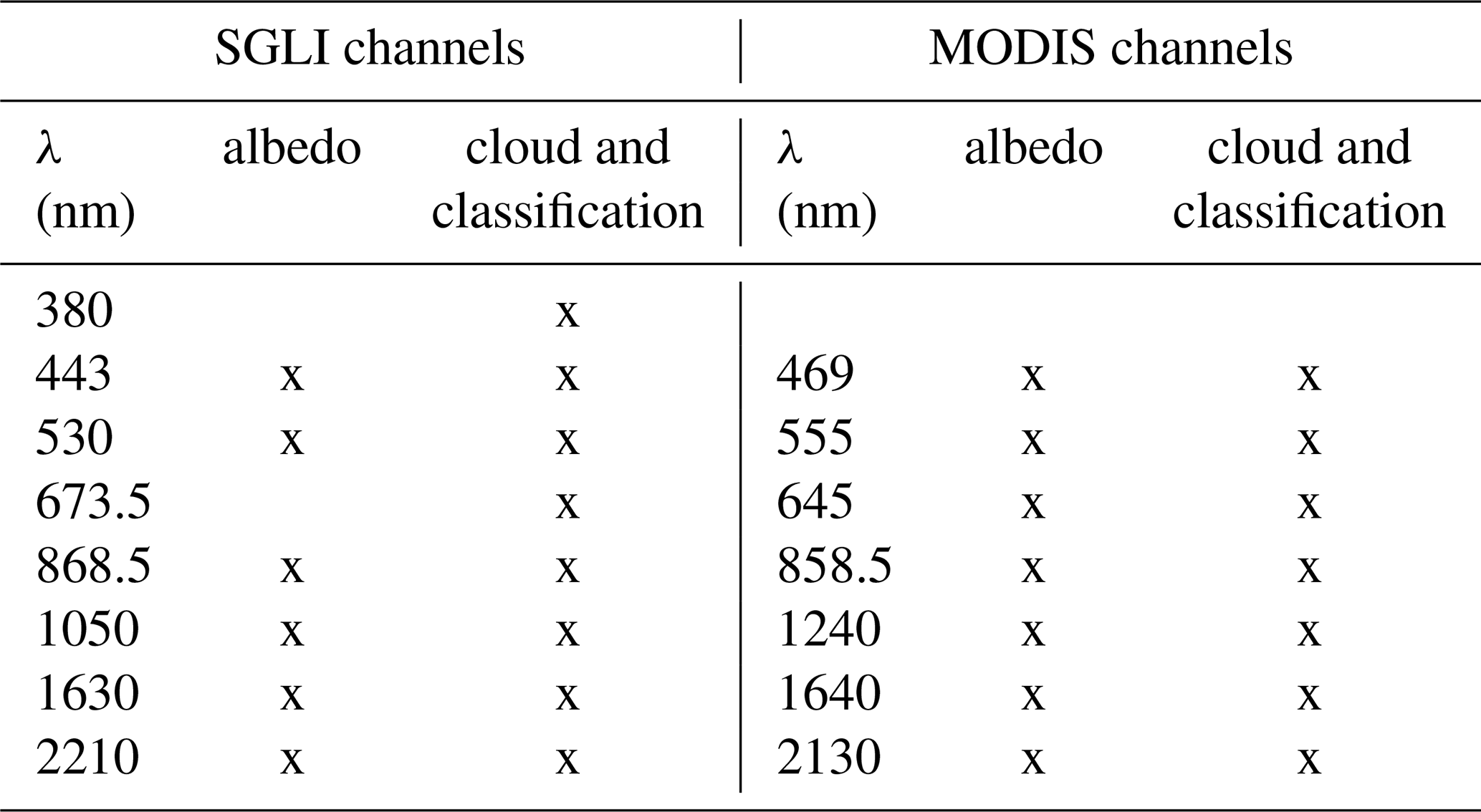
Similar approaches have been used to identify acceptable channels for albedo retrieval. Table 3 lists the MODIS channels that were utilized to retrieve albedo, as well as the Global Change Observation Mission – Climate (GCOM-C)/SGLI channels that were evaluated and eventually employed.²

2.4 Surface classification and cloud filtering

Imperfect cloud screening brings considerable uncertainty to the retrieved sea ice albedo. To mitigate this uncertainty, pixels covered by clouds are detected and removed by a neural-network-based cloud screening and surface classification algorithm (MLCM) developed by Chen et al. (2018). The MLCM (short for Machine Learning Classification Mask) is a threshold-free algorithm trained by extensive radiative transfer simulations. It can be applied to a great variety of surface types to provide reliable cloud mask and surface classification. A comparison between the MLCM and other standard cloud mask algorithms showed that the MLCM is better able to detect cloud edges and deal with high solar zenith angles (Chen et al., 2018). Section 3 indicates that the MLCM can assist in filtering cloud, fog (sea smoke), and hazy atmospheric conditions.

The MLCM is also capable of distinguishing snow-covered sea ice pixels (with a minimum snow depth of 1 cm) from bare sea ice pixels. Independent treatment of classification and albedo retrieval ensures that even on highly heterogeneous surfaces or in conditions where classification of certain pixels is difficult (e.g., the long-standing difficulty in distinguishing between slushy mixtures of ice and water, very thin ice, and melt ponds), the retrieval of their surface albedo values is unaffected.

2.5 Data

2.5.1 Radiance data from the MODIS and SGLI sensors

In this study, the level 1B calibrated radiance data (MOD021) from the MODIS sensor and the infrared scanner (IRS), as well as the near-infrared radiometer (VNR) on the Second-generation Global Imager (SGLI, data available at JAXA, https://gportal.jaxa.jp/gpr/, last access: 18 February 2023), were employed for albedo retrieval and surface classification. While only two sensors are discussed, the retrieval method described in Sect. 2 is generic and applicable to any satellite sensor having suitable radiance data (e.g., the Visible Infrared Imaging Radiometer Suite, abbreviated as VIIRS).

Central wavelengths used by MODIS and SGLI sensors to retrieve albedo and obtain a cloud–surface-classification mask are provided in Table 3. Data in all channels have been aggregated at a common spatial resolution of 1 km.

Table 3 Central wavelengths used by SGLI and MODIS to retrieve albedo and obtain cloud and surface classification mask. The 673.5 nm wavelength channel from SGLI was proven to be saturated and hence was not used to derive albedo.

2.5.2 Independent validation data

Three campaigns conducted in the Arctic provided broadband irradiance data across the Arctic sea ice surface. They are the ACLOUD (Arctic Cloud Observations Using Airborne Measurements During Polar Day) campaign conducted during the 2017 spring–summer transition, the AFLUX (airborne measurements of radiative and turbulent FLUXes of energy and momentum in the Arctic boundary layer) campaign, which took place in April 2019 north of Svalbard, and the MOSAiC (Multidisciplinary drifting Observatory for the Study of Arctic Climate) campaign, which was conducted in late August to September 2020 (Wendisch and Brenguier, 2013; Lüpkes, 2017; IASC, 2016).

With the MLCM, we performed cloud filtering and compared the flight transits to the cloud-free area. By calculating the percentage of cloud coverage (f_c) for the matching dates in the latitude–longitude range of flight operations, only 7 d were found to include clear-sky sea ice observations (f_c≤90 %), and the flight transits were retained (Table 5). Measurements from 2 d during the AFLUX campaign were partly from clear sky, while the remainder were entirely from broken clouds (for a description of the AFLUX data, see Stapf et al., 2021b). The MOSAiC campaign included fewer than 50 valid data points (Jäkel et al., 2021b), all of which were obtained for broken cloud conditions. To eliminate errors caused by dense cloud cover, MOSAiC data were omitted from validation.

During the ACLOUD and AFLUX campaigns, the upward and downward irradiance data (0.2–3.6 µm) were collected by two pairs of CMP-22 pyranometers (Stapf et al., 2019, 2021a). The pyranometers operated at a frequency of 20 Hz and were mounted on the Polar 5 (the ACLOUD campaign used an additional aircraft, Polar 6) research aircraft. Pre-processing was used to avoid data received during high aircraft pitch and roll angles and suspicious equipment frost conditions. Technical details of the pyranometer are provided by Wendisch and Brenguier (2013). Along with the pyranometers on Polar 5 and 6, a Spectral Modular Airborne Radiation measurement system (“SMART albedometer”) on Polar 5 measured spectral irradiances between 0.4 and 2.155 µm at a frequency of 2 Hz during the ACLOUD campaign (Jäkel et al., 2018).

Gröbner et al. (2014), Ehrlich et al. (2019) reported that the pyranometer's uncertainty was less than 3 %, whereas the uncertainty of the SMART albedometer was 7 %.

2.5.3 Pre-processing of validation data

The albedo obtained from SciML has the same spatial resolution as the geolocation data (MOD03), which is 1 km, whereas the aircraft's pyranometers and albedometers have a significantly smaller footprint. As a result, when evaluating SciML models, the estimated albedo is colocated with the MODIS grid and the average value of about 170 measurements from each flight is mapped to a single MODIS pixel. With the MLCM, the pixels with cloud contamination are filtered, and only three surface types were kept in the validation dataset (i.e., sea ice, snow-covered sea ice, and water).

Finally, while the SciML-derived albedo is valid for surface observations, there may be a bias between it and the albedo measured at aircraft height. The Polar 5 and Polar 6 aircraft reached 3000 m height during the mission, and the albedo measurements were therefore influenced by the entire atmospheric layer below the aircraft, resulting in a significant variance in albedo results. To account for the difference caused by the atmospheric constituents, we used the coupled RTM (AccuRT) to simulate the albedo of snow, bare ice, melt pond, and open-water surface at three different levels: surface (α_s), low flight level (α_l, l=350 m), and high flight level (α_h, h=3000 m). Albedo ratios, $r_{\mathrm{l}}=\frac{{\mathit{\alpha }}_{\mathrm{l}}}{{\mathit{\alpha }}_{\mathrm{s}}}$ and $r_{\mathrm{h}}=\frac{{\mathit{\alpha }}_{\mathrm{h}}}{{\mathit{\alpha }}_{\mathrm{s}}}$, were calculated to determine the difference in albedo induced by the atmospheric layer below the flight height.

Figure 2 illustrates the aforementioned spectral and broadband albedos, as well as the ratios. There is significant influence of multiple scattering above the open-water surface due to atmospheric components, particularly in the visible (VIS) range; the albedo at h=3000 m is double that on the surface, whereas the presence of an atmosphere with aerosols results in a decrease in albedo over a bright surface. Among these, the reduction is particularly noticeable in the near-infrared (NIR) band, where air absorption results in a 4 % and 22 % decrease in albedo at low and high levels, respectively. Similar simulation results were found by Jäkel et al. (2021a), using the Two-Stream Radiative Transfer in Snow (TARTES) model (Libois et al., 2013). As can be observed, the difference between low-level and surface albedo is less than 5 %, whereas the difference between high-level and low-level albedo is significantly greater. As a result, we did not use aircraft observations taken above 350 m in order to improve the validation of the “surface” albedo retrieval.

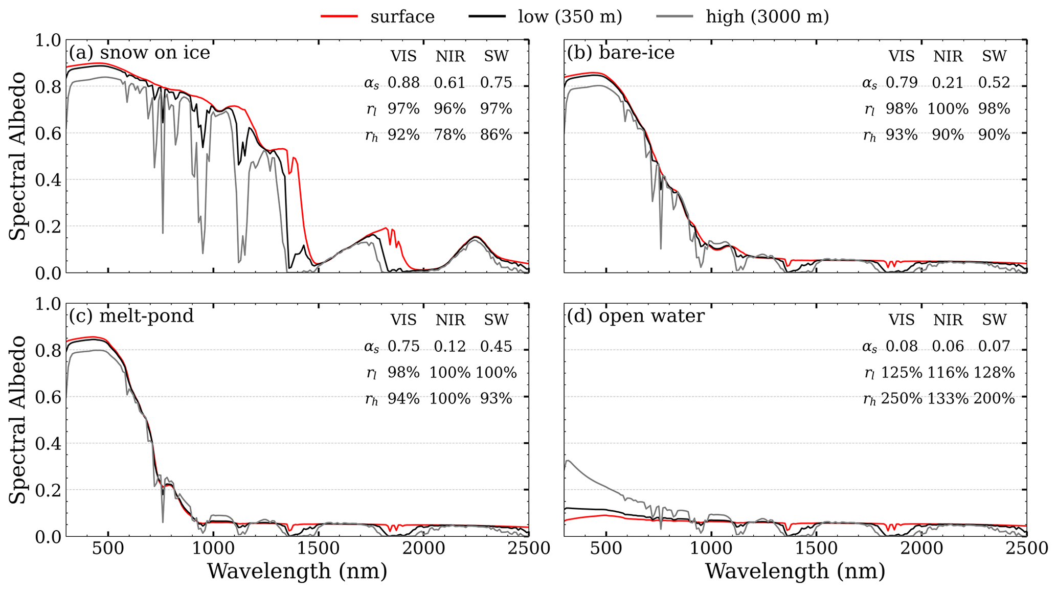
Figure 2 Spectral albedo computed by the RTM at various altitudes (350 m as a black line and 3000 m as a gray line) and the surface (red line).

In all, the selected flight sections are depicted in Fig. 3. Up to four satellite images per day could be employed for retrieval and evaluation in the polar regions. The MODIS transits that correspond to the aircraft operation time and f_c are listed in Table 5.

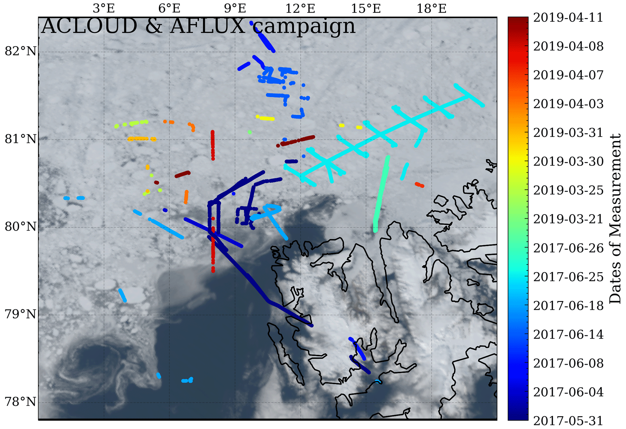
Figure 3 ACLOUD and AFLUX transits of selected flight segments from Polar 5 and Polar 6. The true-color composite from 25 June 2017 is shown in the background. MODIS channels 645, 555, and 469 nm are used as (R, G, B) bands for the true-color RGB. The dates of flight operations are denoted by hues defined by the color bar on the right.

2.5.4 Comparison data

The retrieval results from RTM–SciML models are compared to the currently operational albedo retrieval products listed in Table 1.

• MODIS MCD43D. The 1 km spatial resolution MODIS MCD43D products are the successors to the MCD43B products. The retrievals are performed daily using kernel weights that best represent the majority of situations across the 16 d period, with the day of interest emphasized. MCD43D49-51 corresponds to the black-sky albedo (BSA) for the visible (0.3–0.7 µm, VIS), near-infrared (0.7–5.0 µm, NIR), and shortwave (0.3–5.0 µm, SW) bands, while MCD43D59-61 corresponds to the white sky albedo (WSA) for the three broadband ranges (Schaaf and Wang, 2015b).

• MERIS MPF V1.5 and OLCI MPF V1.5. Istomina et al. (2015); Istomina (2020) developed two albedo retrieval products, utilizing MERIS data from Envisat-1 and Ocean and Land Colour Instrument (OLCI) data from Sentinel-3, respectively. The MERIS sensor was only operational from 2002 to 2012, and the OLCI product is the successor to the MERIS-albedo product (Istomina, 2020); both products are based on the MPD algorithm proposed by Zege et al. (2015). Daily retrieval data are gridded onto a polar stereographic grid with a 12.5 km resolution (the National Snow and Ice Data Center, NSIDC, grid). In Istomina et al. (2015), the MERIS-albedo product was evaluated by comparing the estimated albedo values to aerial measurements from the MELTEX campaign. Landfast ice showed the best agreement, with an R-squared value of 0.84 and an RMSE of 0.068 for 169 matched pixels.

• GLASS (AVHRR) and GLASS (MODIS). Global Land Surface Satellite (GLASS) products are primarily derived from NASA's Advanced Very High Resolution Radiometer (AVHRR) long-term data record and MODIS data, together with other satellite data and auxiliary information (Liang et al., 2021). The sea ice surface albedo in GLASS is derived using the direct-estimation algorithm (Qu et al., 2016); a spatiotemporal filtering algorithm Liu et al. (2013) is utilized to provide gap-free albedo with an 8 d temporal resolution. The spatial resolution of GLASS-albedo retrieved from the AVHRR sensor is 0.05^∘ and from MODIS sensor is 1 km. In Qu et al. (2016), the GLASS (MODIS) product was compared to Tara polar ocean expedition measurements. During the 90 d expedition, the daily average albedo from cruise measurements with around 50 matched retrieval–measurement data points yielded an R² value of 0.67.

• VIIRS L3-SURFALB. Peng et al. (2018) improved the direct-estimation method for sea ice retrieval proposed by Qu et al. (2016) and made it applicable to the VIIRS. The BRDF in Qu et al. (2016) is a weighted average of sea ice, snow-covered ice, and open water, with melt pond conditions omitted. In Peng et al. (2018), all four surface conditions are evaluated and the MPD algorithm is used to derive the BRDF of melt pond. The VIIRS surface albedo (SURFALB) product has been validated using ground truth from the Greenland Ice Sheet and snow-covered land (Peng et al., 2018). Note that the validation data are not applicable to the highly fluctuating sea ice surface; sea ice refers to a floating sheet of ice formed from ocean water, which might be covered by melt ponds or snow during its life cycle. The spatial resolution of both the SURFALB level 2 (L2) granule product and the level 3 (L3) gridded product is 1 km, and the L3 data are used for comparison in this study.

When computing the statistical values (albedo, Pearson r, mean, etc.), the RTM–SciML retrievals are regridded to the same spatial and temporal resolution as their counterparts (e.g., 12.5 km for OLCI/MERIS and 8 d average for GLASS), and if matching validation data are available, the flight measurements are likewise rescaled to the same grids. In retrieval map figures, data are represented with their original spatial resolution. The CLARA-SAL (Karlsson et al., 2012, 2017) and APP-x (Key et al., 2016) albedo products produced from the AVHRR sensor are also provided for reference.

2.6 Scientific machine learning (SciML) model

Neural network models, specifically models with the multi-layer artificial neural network (MLANN) structure, have been demonstrated to be useful for retrieving and estimating snow and sea ice parameters. Successful implementations include the sea ice and snow thickness retrievals using microwave data (Herbert et al., 2021; Hu et al., 2021; Zhu et al., 2021; Wang et al., 2020; Braakmann-Folgmann and Donlon, 2019; Lee et al., 2019; Tedesco and Jeyaratnam, 2016; Cao et al., 2008; Tedesco et al., 2004), and sea ice concentration (SIC) or melt pond fraction (MPF) retrievals using radiance or reflectance data (Chi et al., 2019; Karvonen, 2017; Rösel and Kaleschke, 2012).

A MLANN's computational unit is a neuron (alternatively called a perceptron), which is organized in a network topology. A set of functions $f_j(x;{\mathbf{w}}_j,{\mathit{b}}_j)$ connected in a chain can be used to describe the architecture of a fully connected neural network with n layers in total (including the input and output layers):

$$\begin{array}{}\text{(1)}& F\left(y\right)=f_n\left(\mathrm{\dots }{f}_{\mathrm{3}}\left(f_{\mathrm{2}}\left(f_{\mathrm{1}}\left(x\right)\times w_{\mathrm{1}}+b_{\mathrm{1}}\right)\times w_{\mathrm{2}}+b_{\mathrm{2}}\right)\mathrm{\dots }\right).\end{array}$$

The previous layer's output is transformed by $f_j\left(x\right)\times {\mathbf{w}}_j+{\mathit{b}}_j$, and then an activation function f_j+1 (which is typically non-linear) is applied to perform an element-wise operation.

Generally, as the network grows deeper, the features become more abstract and complicated, as each succeeding layer is constructed from the already transformed features of the prior layer (LeCun et al., 2015). The network's n−2 hidden layers enable it to describe nonlinear relations between the independent and dependent variables (x,y). The matrices w_j define the weights for linear transformations between layers, whereas the vectors b_j define the biases. The final layer (output layer) has three neurons encoding the predicted albedo values (${\widehat{\mathit{\alpha }}}_{\mathrm{VIS}}$, ${\widehat{\mathit{\alpha }}}_{\mathrm{NIR}}$, ${\widehat{\mathit{\alpha }}}_{\mathrm{SW}}$).

Neural network models with different configurations are trained using 80 % of the SD, and the portion of the SD that was not included in the network training process was held out for validation (the “out-of-sample validation” step shown in Fig. 1). To obtain an efficient MLANN, both the network structure's topology and hyperparameters should be tweaked properly.

A stochastic gradient descent (SGD) optimization is used to update the weights and biases in an MLANN during back-propagation. To perform the SGD, the adaptive moment estimation (Adam, Kingma and Ba, 2014) was chosen, which trains the models in 200 epochs with a batch size of 64. A MLANN's hyperparameters include the learning rate and the activation function. To determine the optimal learning rate, Bayesian optimization was employed (Brochu et al., 2010), and the rectified linear units (ReLU, Nair and Hinton, 2010) were used as the activation function in the hidden layers. Batch normalization (Ioffe and Szegedy, 2015) is performed to enhance the MLANN's generalization capabilities and make the network less sensitive to random initialization of the weights and biases (Santurkar et al., 2019). To avoid overfitting, dropout layers (Srivastava et al., 2014) were included as a regularization for networks with more than two hidden layers. In our evaluation, dropout layers with a rate of 0.2 were found to be optimal, implying that one in every five inputs is randomly eliminated from each update cycle.

The network structure with three hidden layers was shown to perform well when evaluated using the hold-out dataset (the 20 % of SD).³ Furthermore, when these MLANNs were applied to the MODIS sensor, the distributions of their retrieval results were very comparable (see Fig. B1b). Consequently, the “winning model” was determined by comparing the retrieval results of each candidate against independent validation data. The independent validation data for the MODIS sensor were derived from pyranometer measurements described in Sect. 2.5.2, and 4000 entries were sampled from the total dataset (N=7964). The $\mathrm{16}\times \mathrm{10}\times \mathrm{8}$ network topology demonstrated a slight overall performance advantage (Table B1). ⁴ The final retrieval model for the SGLI sensor was determined by comparing the R² of SGLI and MODIS retrieval results from the same day ⁵.

As a final note, the SMART albedometer measures within a narrower irradiance range (as compared to pyranometer). Therefore, a separate MLANN model was trained utilizing broadband albedo from different ranges (i.e., modifying the irradiance ranges of the SD in the “integrate” stage of Fig. 1). The difference in wavelength range is summarized in Table 4. Throughout the text, the two models are discussed separately: (a)–(c) of Figs. 4 and 9, as well as Fig. 7a, are broadband albedo values with adjusted ranges, while the remainder of the discussion pertains to the 300–2500 nm broadband.⁶

Table 4 Difference between the wavelength ranges of the retrievals from the two MLANN models. The validation of retrieval results are shown in Figs. 3 and 6 and Table A2.

3 Validation

3.1 Validation of MODIS-retrievals

Polar-orbiting satellites transit the two polar areas up to four times per day, and cloud-free retrievals from all transits (Table 5) are used to compare with the independent validation data measured on Polar 5 and Polar 6 aircraft. Due to the absence of a time constraint on the retrieval data, a single gridded airplane measurement can match many satellite retrievals.

Table 5 Time stamps for airborne observations, satellite overflights in UTC, and cloud pixel percentages in the latitude–longitude ranges of aircraft during the ACLOUD and AFLUX campaigns (77.8–82.4^∘ N, and −0.25–20.5^∘ E). Note that days with only broken-cloud observations (cloud coverage greater than 90 %) are not included in the table.

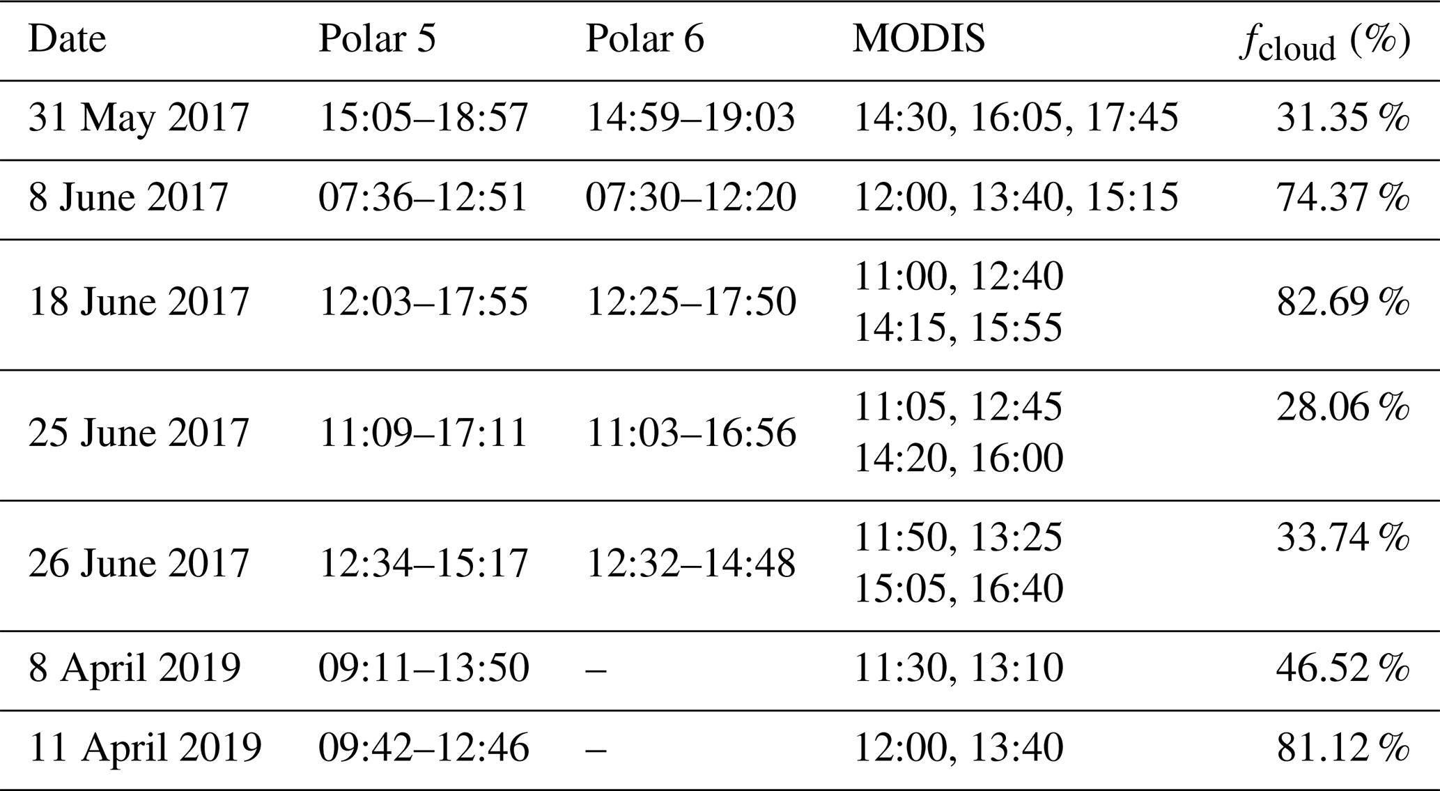
Figure 4 indicates that the RTM–SciML retrieval method is capable of producing satisfactory albedo outputs with low errors and high Pearson r coefficients. The agreement between the retrieved shortwave albedo and the pyranometer-measured albedo is better than with the albedometer; the regression line (marked in red) connecting the pyranometer-measured albedo and the retrieval almost completely overlaps the (0,1) line, indicating a perfect one-to-one correspondence. Note that due to the addition of data from two aircraft during the ACLOUD campaign and two flights from the AFLUX campaign, the acquired pyranometer data are twice as extensive as the albedometer measurements (7964 versus 3936).

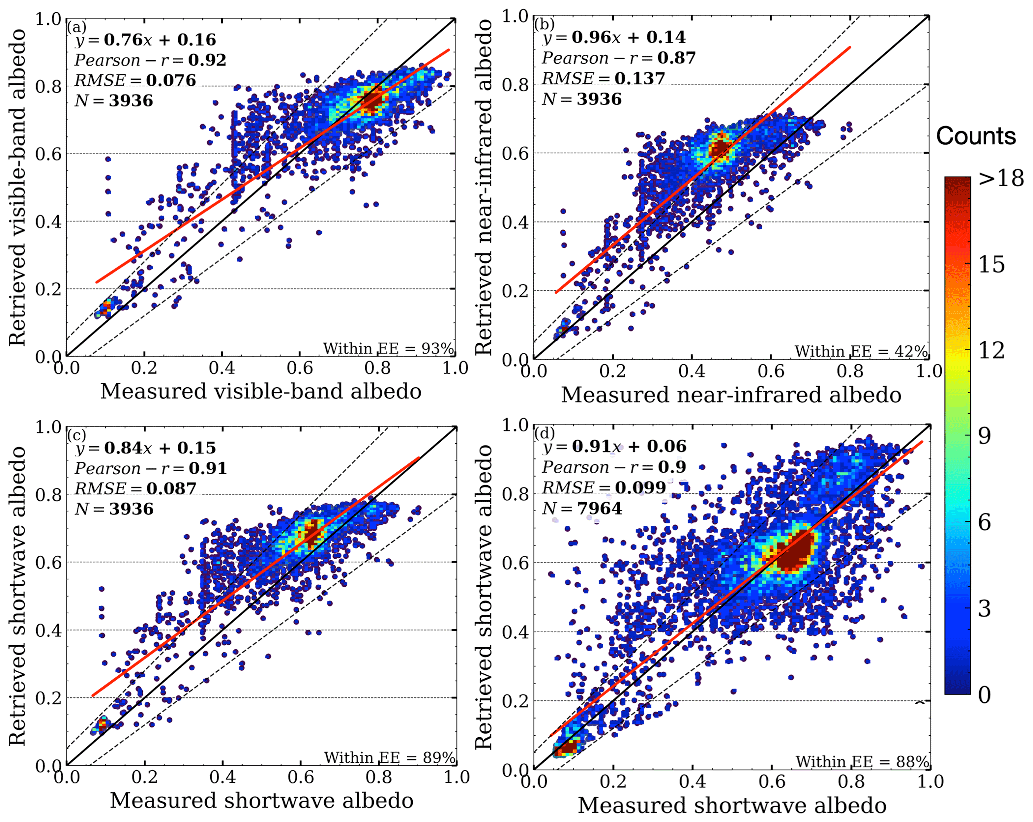
Figure 4 Correlation between ACLOUD-AFLUX albedo measurements and MODIS overflight. The comparisons with the albedometer in the VIS, NIR, and SW ranges are shown in panels (a)–(c), whereas panel (d) shows the comparison with the pyranometer. The wavelength range difference between the two instruments and the corresponding retrieval models can be found in Table 4. The color scheme indicates the density of the numbers. The correlation equation ($\widehat{y}=a\cdot y+b$), Pearson r coefficient (r), root-mean-square error (RMSE), the percentage of data within a 15 % expected error (f_EE≤15), and number of pixels (N) used to compute the statistics are provided in all panels. The red lines represent the linear correlation between $\widehat{y}$ and y, the solid black lines represent $(\mathrm{0},\mathrm{0})-(\mathrm{1},\mathrm{1})$, and the dashed black lines represent the 15 % error range.

The highest inaccuracy of retrieval occurs in the near-infrared band: around 15 % over-estimation for bare sea ice and snow-covered ice pixels. Apart from the larger positive bias inherent in the SciML algorithm (as compared to the visible band), the disparity in NIR values could be partly caused by the measurement uncertainty; the albedometer's overall uncertainty in the near-infrared wavelength band is reported to be the greatest (Jäkel et al., 2021a). It is also worth noting that even though the comparison is confined to low-level (≤ 350 m) flight measurements, there is still a non-negligible height-induced error in the NIR values (refer to the RTM simulation findings in Fig. 2): on snow-covered sea ice, the error is −4 % (lower than the surface), which increases the gap between the retrieval (of ground) and the measurements (of low-altitudes). For open water, the near-infrared albedo at 350 m is +16 %.

Overall, as illustrated in Fig. B2, the correlation coefficients for snow-covered ice and open water are relatively high across the wavelength ranges (r=0.75 and r=0.81, respectively), whereas the correlation coefficients for bare sea ice and ice with melt pond coverage are lower (r=0.54). The reason is that in contrast to the more stable glacier, sea ice is more variable. For the days covered, the mean time discrepancy between MODIS transit and flight measurements is about 2 h, with a maximum time difference of 3–5 h (4, 4.85, and 3 h for 31 May, 8 June, and 25 June, respectively).

When a time window of 1.5 h was used for time restriction, a greater degree of agreement and smaller error was found; evaluating against pyranometer data (N=4144) reveals r of 0.92 and RMSE of 0.094 for the shortwave albedo retrieval (Model 1), and evaluating with albedometer data (N=1225) shows r of 0.93, 0.89, 0.92 and RMSE of 0.069, 0.143, 0.085, in the visible, near-infrared, and shortwave bands, respectively (Model 2).

In our most recent work, the RTM–SciML retrievals from the MODIS sensor in the Okhotsk region between 2002 and 2014 are validated using Soya icebreaker data. With a 1 h time window (N=359), the RMSE is 0.097, and with a 3 h time window (N=911), the RMSE is 0.11.

3.2 Validation of SGLI retrievals

Frequently, fog (sea smoke) forms above sea ice and polynyas (Vihma et al., 2014). On 8 April 2019, data taken south of 80.6^∘ N were in such a condition. On 11 April, a thick cloud with a sharp edge moved from 15^∘ E at 05:50 UTC to 7^∘ E at 12:25 UTC (Stapf et al., 2021b). As seen in the RGB and surface classification images (Fig. 5), the fog from 8 April and the cloud from 11 April was correctly identified by the MLCM for both sensors.

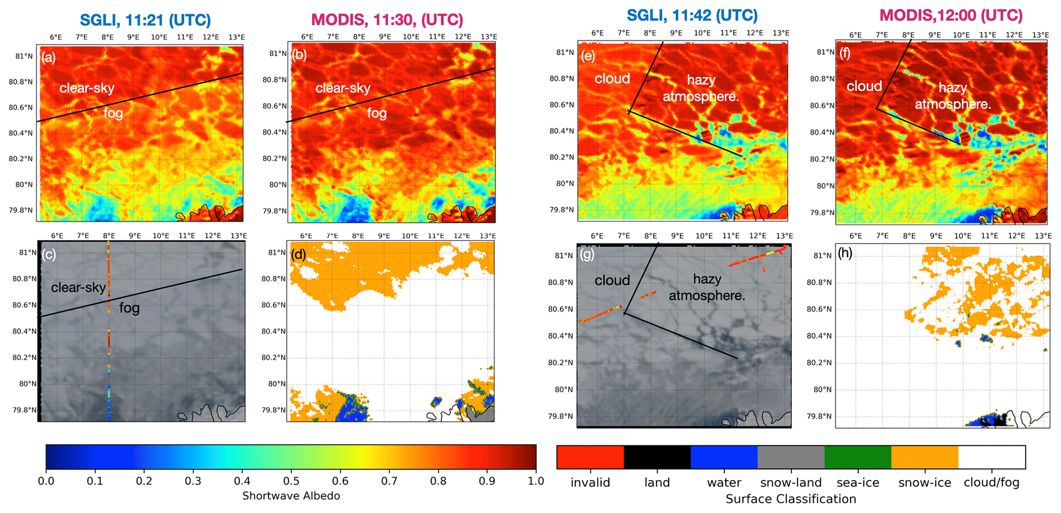
Figure 5 Albedo retrieval maps, RGB maps, and surface classification maps from 8 April 2019 (a–d) and 11 April 2019 (e–h). Panels (a) and (e) represent the albedo values retrieved with the SGLI sensor, (b) and (f) represent the albedo values retrieved with the MODIS sensor, (c) and (g) represent the spatial overlay of surface albedo measurements made on low-level (≤ 350 m) flights (dots) on true color composite images, and (d) and (h) represent the surface classification results. The black lines represent the distinctions between various atmospheric conditions.

On 11 April, the cloud-free area was seen to have a hazy atmosphere (Stapf et al., 2021b), and RTM models showed a thick aerosol optical depth of 0.065 (wavelength unspecified). The MLCM also detected the haze, which was classified in Fig. 5 as “cloud/fog”. Figure 5 indicates that, even with the impact of cloud, fog, or hazy atmosphere, the SGLI- and MODIS-retrieved albedo values (α) for different surface types are within reasonable ranges: melt pond (α≤ 0.3), bare sea ice (α≈ 0.6), and sea ice with snow coverage (α≥ 0.7). When compared to data from low-level (≤ 350 m) aircraft at the same location and to cloud-free MODIS retrievals (Fig. 5), the values are largely consistent.

The scatter plot in Fig. 6 illustrates the correlation between the measured and retrieved albedo (under clear-sky conditions on 8 April) using SGLI-channel and MODIS-channel radiances. Both results were derived with the same retrieval methods as those outlined in Sect. 2. For retrievals using SGLI data, 82 % of the data were under the 15 % expected error (EE), demonstrating a higher degree of agreement than the results produced from MODIS radiance data for this date. Correlation coefficients of 0.984 and 0.892, as well as RMSE of 0.082 and 0.136, indicate that RTM–SciML models can produce satisfactory results for cryosphere surface albedo retrieval.

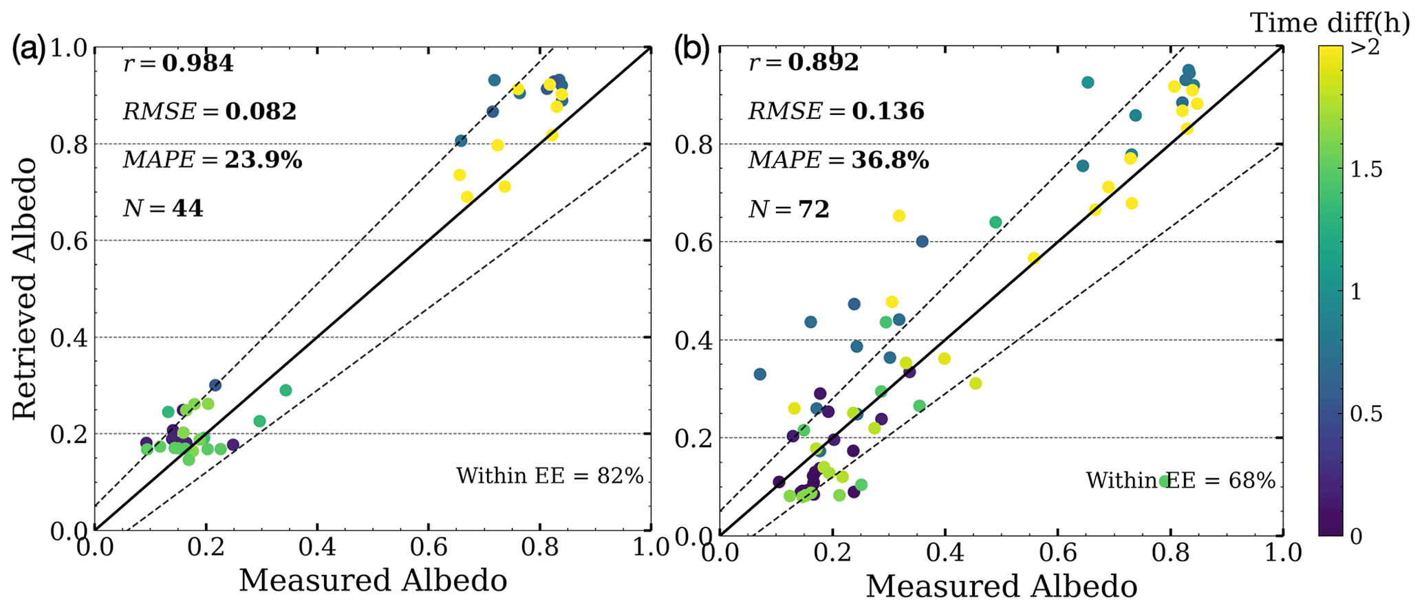
Figure 6 Correlation between shortwave albedo measurements from the AFLUX campaign and satellite overflight (SGLI a, and MODIS b), 8 April 2019. The color indicates the time interval between campaign measurements and satellite overpass. The Pearson r coefficient (r), root-mean-square error (RMSE), mean absolute percentage error (MAPE), and the number of pixels (N) used to calculate the statistics are provided in each panel.

4 Discussion on the source of validation error

Independent of the surface type or spectral range, all of the evaluations outlined above are prone to uncertainty due to equipment error, cloud contamination, surface metamorphism (drift and melt or refreeze), and differences in observation height, footprint, and solar zenith angle (SZA).

In the following discussion, we will break down and analyze the errors by their sources. The data were subjected to a more stringent temporal constraint of δ_t=1.5 h in order to allow for a more precise characterization of specific sources of inaccuracy. Figure 7 depicts the percentage difference between the observed and retrieved shortwave albedo when a maximum time difference between aircraft and satellite of 1.5 h is allowed. Still, the percentage difference between the RTM–SciML estimated values and pyranometer measurements are smaller than those with albedometer measurements. Meanwhile, the error for the open-water surface (flight segments within the dashed red line) is significantly larger when compared to the albedometer data than when compared to the pyranometer data.

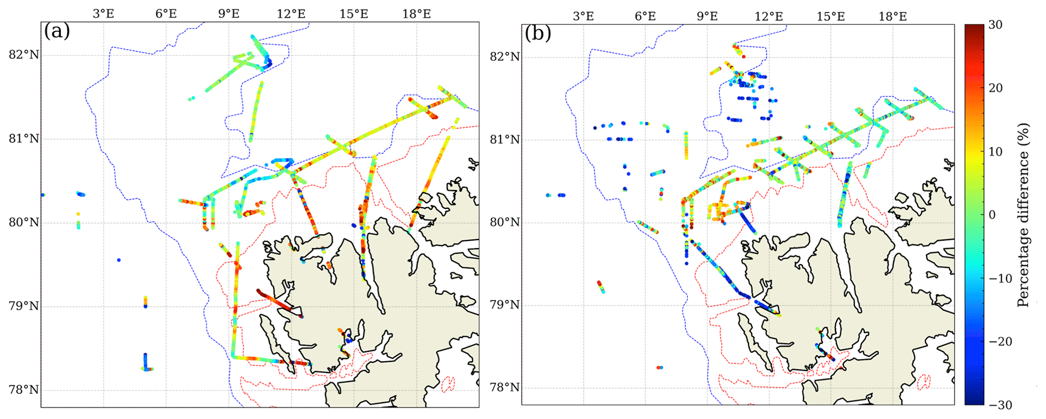
Figure 7 A map illustrating the percentage difference between the RTM–SciML estimated broadband albedo and the albedo measured in situ using (a) the “SMART” albedometer and (b) the pyranometer. To choose the matching MODIS retrieval, a tight time constraint of 1.5 h (δ_t≤1.5 h) was applied. On the right, the color bar indicates the scale of the percentage difference value for each pixel ($\frac{\widehat{y}-y}{y}\cdot \mathrm{100}$ %). Additionally, dashed red and blue lines represent the 200 and 1000 m isobaths, respectively. Each flight segment's dates are listed in Fig. 3.

4.1 Distinction in the footprint of observation

When aircraft measurements are up-scaled to MODIS footprints, around 170 aircraft measurements were taken to match one satellite pixel. According to prior research, an albedo line 100 m long surrounding melt ponds would have a standard deviation of roughly 0.4 (Perovich, 2002), while the albedo of thin ice inside a grid cell would have a standard deviation of up to 0.29 (Lindsay, 2001). Due to the fact that measurements along the aircraft transit do not accurately reflect the area's average albedo (as determined by satellite sensors), the uncertainty introduced by different observation footprints (i.e., subpixel effects) is not negligible but difficult to quantify. On a homogeneous surface such as fresh snow, subpixel effects could be small, but for the heterogeneous surface consisting of a snow–ice–water mixture, the influence is large.

4.2 Cloud contamination effects

While cloud screening eliminates cloudy pixels in satellite data, data acquired during airplane flights are not corrected for cloud cover. Given that more than one-third of the operational spatial range is obscured by clouds, it is possible that some pixels labeled as “clear sky” by the MLCM are cloud-contaminated pixels as a result of (i) a time mismatch between the MODIS overpass and aircraft data collection or (ii) simply imperfect cloud screening. Multiple reflections between the surface and cloud base would introduce uncertainty into the albedo measured by the airplane.

Figure 8 Histograms of the shortwave albedo measured during the cloud-free ACLOUD-AFLUX flights (red columns) and the RTM–SciML's corresponding retrieval (gray columns). To choose the matching MODIS retrieval, a tight time constraint of 1.5 h (δ_t≤1.5 h) was applied. The dates are displayed at the top of each panel. Additionally, the upper-right corner displays the cloud fraction (f_cloud), the percentage of data within 15 % expected error (f_EE≤15), the root-mean-square error (RMSE), and the number of pixels for each evaluation (N). Due to a lack of appropriate data, all AFLUX measurements were combined together for examination, as illustrated in panel (f).

As illustrated in Fig. 8, the agreement is negatively correlated with cloud coverage, with the exception of Fig. 8b. On 8 June 2017, the date depicted in panel Fig. 8b, a considerable decrease in temperature and an increase in liquid water vapor (IWV) were recorded (Wendisch et al., 2019). Following a day of dense cloud cover, the surface temperature measured on ice floe camps increased by 2^∘ on 10 June 2017 (Barrientos Velasco et al., 2018). A Magna probe (Sturm and Holmgren, 2018) recorded that snow depths on the ice floe on 14 June were down to 22 ± 18 cm (with 32 % of data below 10 cm), while on 5 June the snow depth was 37 ± 24 cm (with 9 % of data below 10 cm) (Jäkel et al., 2019). These data indicate that the surface conditions changed radically around 8 June, which possibly led to the larger root-mean-square error (RMSE of 0.149). The RMSEs are all minor on the 3 d with significantly less cloud cover (Fig. 8a, d, and e). The best agreement occurs on 25 June, when an analysis of 2245 accessible MODIS pixels reveals an error of only 0.066; 96 % of the data are within an error of 15 %.

The spatial overlay of observations from 25 June 2017 on a retrieval image utilizing MODIS's 12:45 UTC transit is shown in Fig. 9. Snow-covered ice, open water, and bare-ice albedo values are all within acceptable limits and are in good agreement with albedometer and pyranometer determinations.

Figure 9 (a–c) Spatial overlay of albedometer measurements on top of the RTM–SciML-derived albedo in the VIS, NIR, and SW ranges from 12:45 UTC on 25 June 2017. (d) Spatial overlay of pyranometer measurements on the RTM–SciML-derived SW albedo. (e) Spatial overlay of aircraft altitudes on the true-color composite. (f) Surface classification results. Cloud-contaminated pixels (shown in white in f) were removed during the retrieval.

4.3 Albedo variations caused by changes in the solar zenith angle

Fortunately, the latitude–longitude range experienced clear skies for 3 consecutive days during the campaign, i.e., from 24 to 26 June 2017. The data from four MODIS overflights per day (see Table 5) can be used to determine changes in surface albedo caused by changes in solar zenith angle and surface metamorphism.

Visual examination of the RGB images of the eight MODIS transits from 24 to 25 June revealed no apparent ice drift during the 2 d (refer to the accompanying GIF image in the Supplement). Following this, we employed the MLCM to filter out cloud-contaminated regions during any of the four MODIS transits on 25 June. In other words, assuming there is no ice drift, the changes in albedo value over the period of four satellite transits are due to either surface metamorphism or a shifting solar zenith angle.

The probability density functions (PDFs) of the surface albedo in the region shown in Fig. 9 were produced using the selected data (Fig. 10a). A Gaussian kernel probability density (Turlach, 1993) was used to estimate the PDF. The probability of albedo values falling within the interval $\mathrm{P}(a<x\le b)$ is measured by subtracting the two integral values $\mathrm{P}(a<x\le b)=F_x\left(b\right)-F_x\left(a\right)={\int }_a^{b}f\left(x\right)\mathrm{d}x$, where F(x) is the cumulative density function (CDF) and f(x) is the PDF. The area between the PDF curve and the x axis is equal to 1 (Scott, 2015). The bimodal distribution with one mode at 0.1 and the other at 0.65 indicates that the most prevalent surface types are water and snow-covered sea ice, with bare ice accounting for a small portion of the data.

We noted the difference in SZA over the four MODIS transits, from 55–59 at 11:05 UTC to a higher value of 61–65 at 16:00 UTC, and the difference increased the albedo for snow and water by 6 % and 30 %, respectively, while the values on the bare-ice surface remained relatively stable (5 % fluctuations).

The variations in albedo caused by increasing SZA were investigated in RTM simulations (see the inset table in Fig. 10b). The relevant parameters for the simulation are snow thickness (h_s=0.2 m), effective grain size of snow (r_e=100 µm), pond depth (h_w=0.1 m), and black carbon impurity fractions for snow and ice ($f_{\mathrm{bc}}=\mathrm{1.0}\times {\mathrm{10}}^{-\mathrm{7}}$). Although the difference in broadband albedo values indicates that the snow, ice, and water conditions in the RTM simulations do not match the surface conditions at this location, they may serve as a reference for the portion of the albedo difference caused by SZA, which is 2.7 %, 50 %, and 4 % for snow-covered ice, water, and bare ice, respectively. With these numbers in mind, we can conclude that the lower variance in snow and ice surface albedo (despite increasing SZA) and the less noticeable increase in water albedo are both related to surface melting.

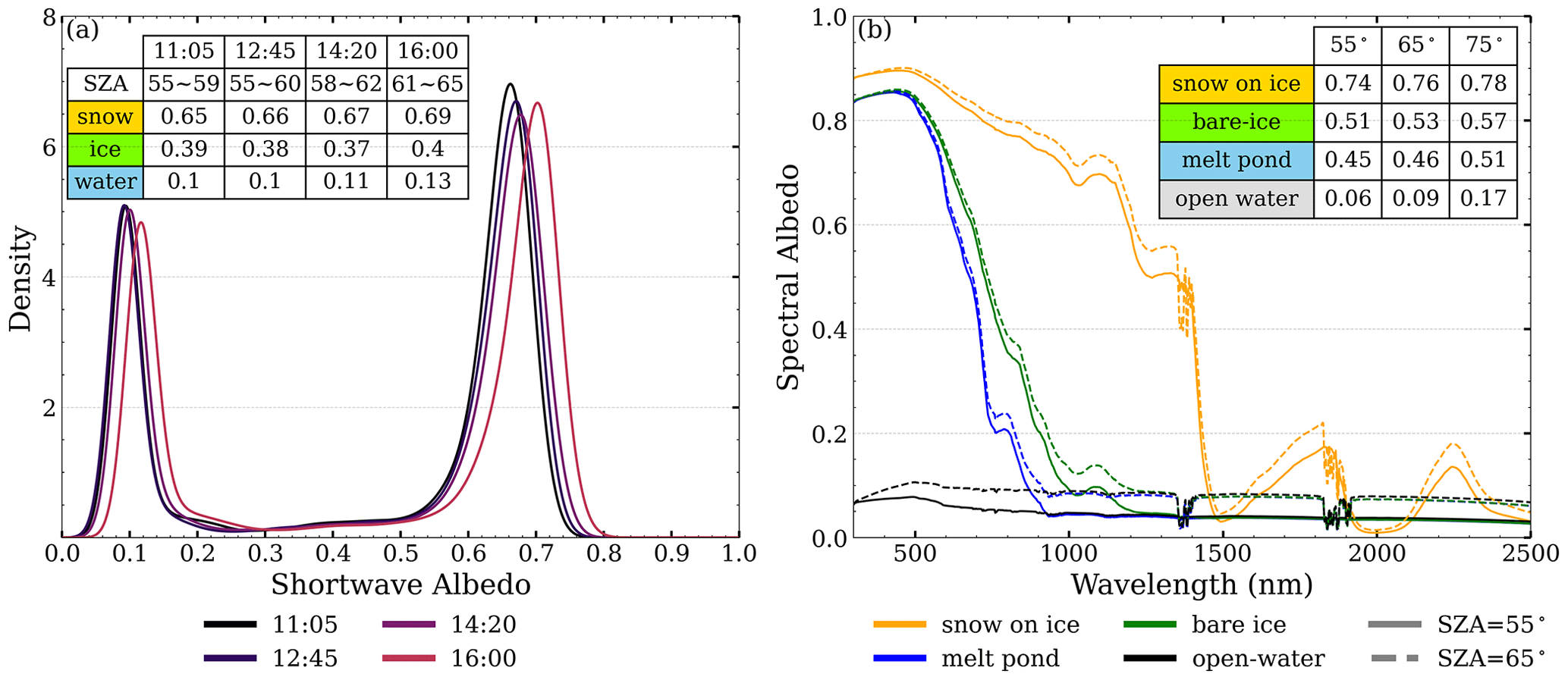
Figure 10 (a) Probability density curves of albedo on 25 June. The colors denote the retrievals from several MODIS overflights. The average albedo estimated for each surface and solar zenith angle (SZA) ranges are provided in the inset table. (b) RTM-simulated spectral albedo of snow, melt pond, bare ice, and open water; dashed and solid lines indicate spectral albedo with varying SZA. The inset table shows the calculated shortwave albedo of each surface and SZA pair.

4.4 Changes in albedo as a result of surface metamorphism

To analyze the fluctuation in albedo caused by surface metamorphism (intra-daily variation due to snow melting, pond development, or pond drainage), we picked the “consistently clear” latitude–longitude coordinates throughout the eight MODIS overflights over a 2 d period. The pixels that have been filtered out due to cloud cover happen to be snow cases. As a result, the following analysis focuses on the phase transitions at the marginal sea ice zone, which is a system composed of bare ice thicker than 30 cm (typical albedo values between 0.4 and 0.5, Brandt et al., 2005; Petrich and Eicken, 2009), melt ponds (typical albedo values between 0.2–0.4, Grenfell and Maykut, 1977; Grenfell and Perovich, 1984; Grenfell, 2004; Petrich and Eicken, 2009), and open water (typical albedo below 0.2, Toyota et al., 1999; Petrich and Eicken, 2009).

Figure 11 depicts the distribution of albedo values at the eight MODIS overflights. Comparing the distributions of α₂₄ and α₂₅ at the same SZA (i.e., the first two columns of Fig. 11), the histograms appear to have a similar shape. However, the change in albedo at a fixed location over about 24 h (Δ_α, the third column of Fig. 11) can be as significant as 0.4. As no apparent ice drift was observed and the location was at the intersection between open-water and sea ice regions, this circumstance indicates that the surface was undergoing intermittent melting and refreezing, akin to the situation of a polynya.

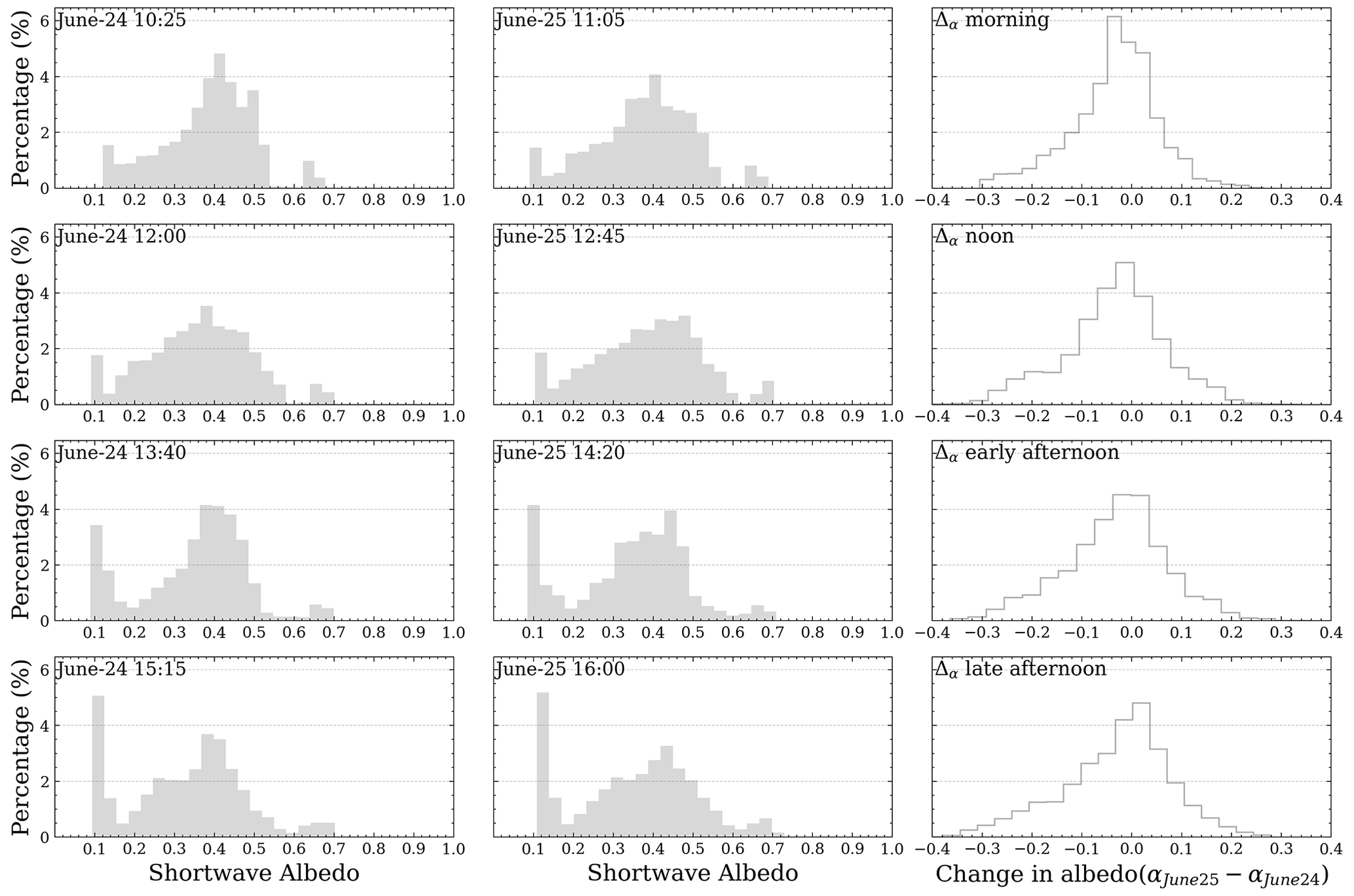
Figure 11 Histogram of the distribution of albedo values observed during the eight MODIS overflights on 24–25 June. The albedo histograms for 24 June (α₂₄) and 25 June (α₂₅) and the difference (${\mathrm{\Delta }}_{\mathit{\alpha }}={\mathit{\alpha }}_{\mathrm{25}}-{\mathit{\alpha }}_{\mathrm{24}}$) are shown in the columns from left to right. From top to bottom, the rows represent the four satellite overpasses that occurred throughout the day: in the morning, at midday, in the early afternoon, and in the late afternoon.

To summarize, in Sects. 3–4, we evaluated the RTM–SciML retrieval results using in situ measurements. The uncertainties associated with the evaluation were explained in detail (per source of error) in order to evaluate their impact. Despite these uncertainties, the current technique for albedo retrieval, which is based on (1) an AccuRT-generated SD and (2) a SciML model trained using the SD as prior knowledge, can indeed produce reasonable albedo outputs, with a RMSE of 0.094 evaluated on over 4000 pyranometer measurements under clear-sky conditions.

5 Comparison of RTM–SciML retrievals with the existing methods

In this section, the RTM–SciML albedo retrievals are compared with the products listed in Table 1. A brief description of the relevant products and sensors are provided in Sect. 2.5.4.

5.1 Comparison with the MCD43D49∼51 BSA products

MODIS MCD43 is a land albedo product; only a small amount of sea ice surface albedo is available near the shore (in the “shallow ocean” zone denoted by the BRDF/Albedo Quality Product, MCD43A2, Schaaf and Wang, 2015a). While prior research has validated the albedo product for glacier, tundra, and snow-covered land surfaces, the small amount of sea ice albedo on the shallow ocean has not been validated previously (Ren et al., 2021; An et al., 2020; Pope et al., 2016; Wang et al., 2012). Using ACLOUD-campaign measurements, the MCD43's reliability in the sea ice zone may be assessed.

On the same days, Figs. 12 and 13 compare the RTM–SciML-derived broadband albedo values utilizing MODIS TOA radiances (i.e., MOD021KM) as input to the MCD43-derived BSAs. The RTM–SciML-derived albedo values represent the average of all available clear-sky pixels observed across four MODIS transits within the day, whereas the MCD43 product is representative of the albedo at local noon (Stroeve et al., 2005). Therefore, values from the MCD43 product are expected to be slightly lower than the RTM–SciML results due to the relatively low solar zenith angle (52–55^∘). We need to highlight that the two comparisons are made at different wavelengths (the NIR and SW upper bounds for RTM–SciML and MCD43 albedo are 2.8 and 5 µm, respectively) and with different albedo assumptions (blue-sky and black-sky albedo for RTM–SciML albedo and MCD43 albedo, respectively). All albedo maps include superimposed SMART albedometer measurements from the ACLOUD campaign (Jäkel et al., 2018) as a reference. Note that the flight segments that overlapped with MCD43D retrievals in Fig. 12 were at an altitude of h≥2500 m, indicating that the validation data on open-water surfaces have a 33–150 % positive bias relative to the surface albedo values; the biases for bare-ice and snow-covered ice surfaces are −10 to −7 % and −22 to −8 %, respectively (see flight heights in Fig. 9e and the height-induced bias in Fig. 2).

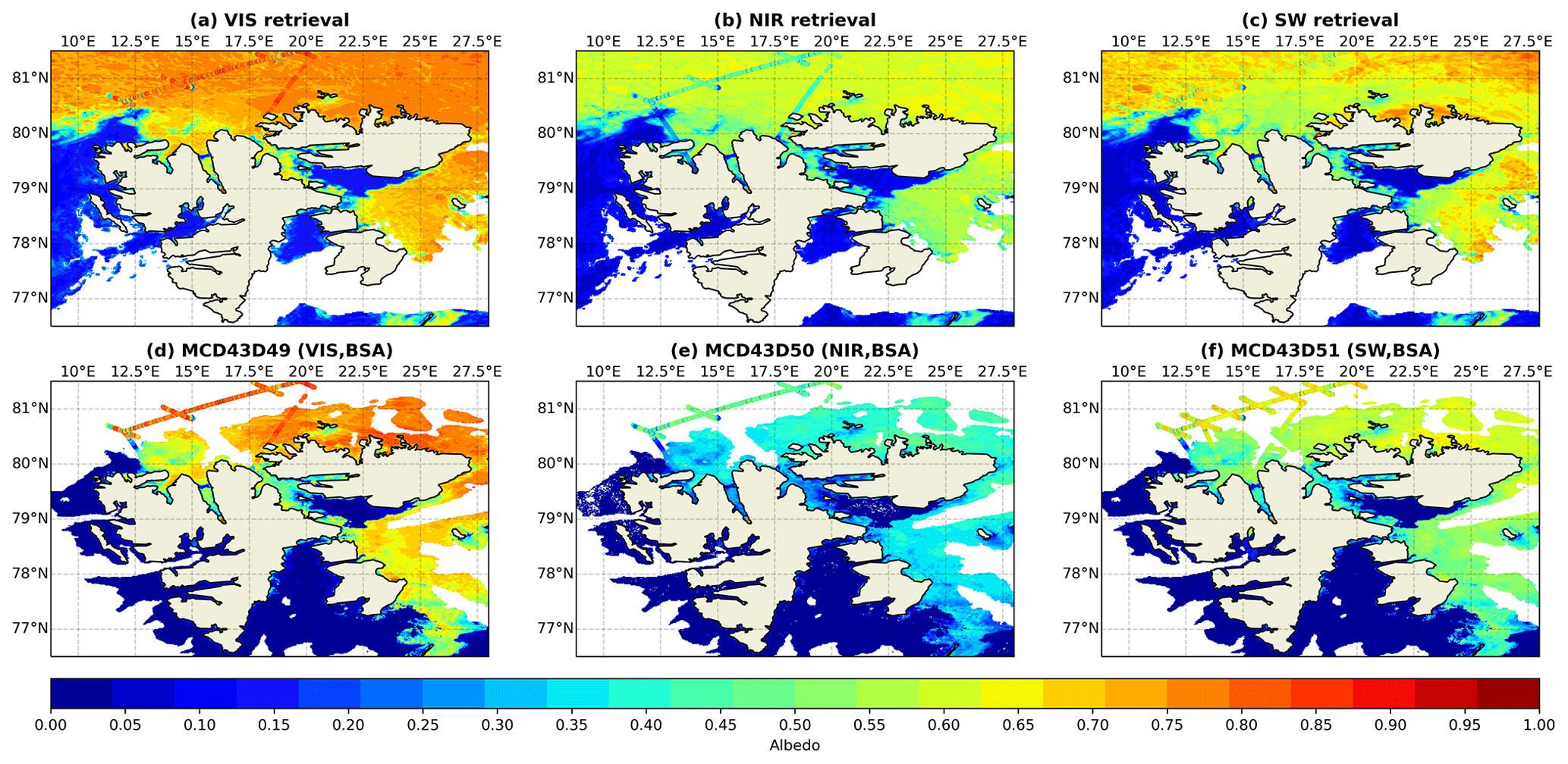
Figure 12 Albedo retrieval maps on 25 June 2017 in the shallow-ocean region near Svalbard. The albedometer measurements from the ACLOUD campaign are superimposed over the retrieval maps in each panel. Note that both low- and high-level flight measurements are included. (a–c) The visible, near-infrared, and shortwave (VIS, NIR, SW) albedo values derived using the RTM–SciML-albedo product and MODIS radiance data. (d–f) The three broadband black-sky albedo values (BSAs) derived by MCD43D49-51. The empty regions in panels (a) to (c) correspond to cloud coverage throughout the day on 25 June 2017, whereas the empty regions in panels (d) to (f) correspond to ocean areas where MCD43 does not provide retrievals.

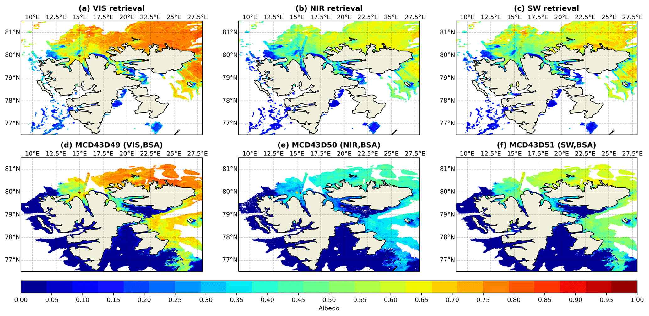
Figure 13 Albedo retrieval maps similar to Fig. 12 but on 26 June 2017.

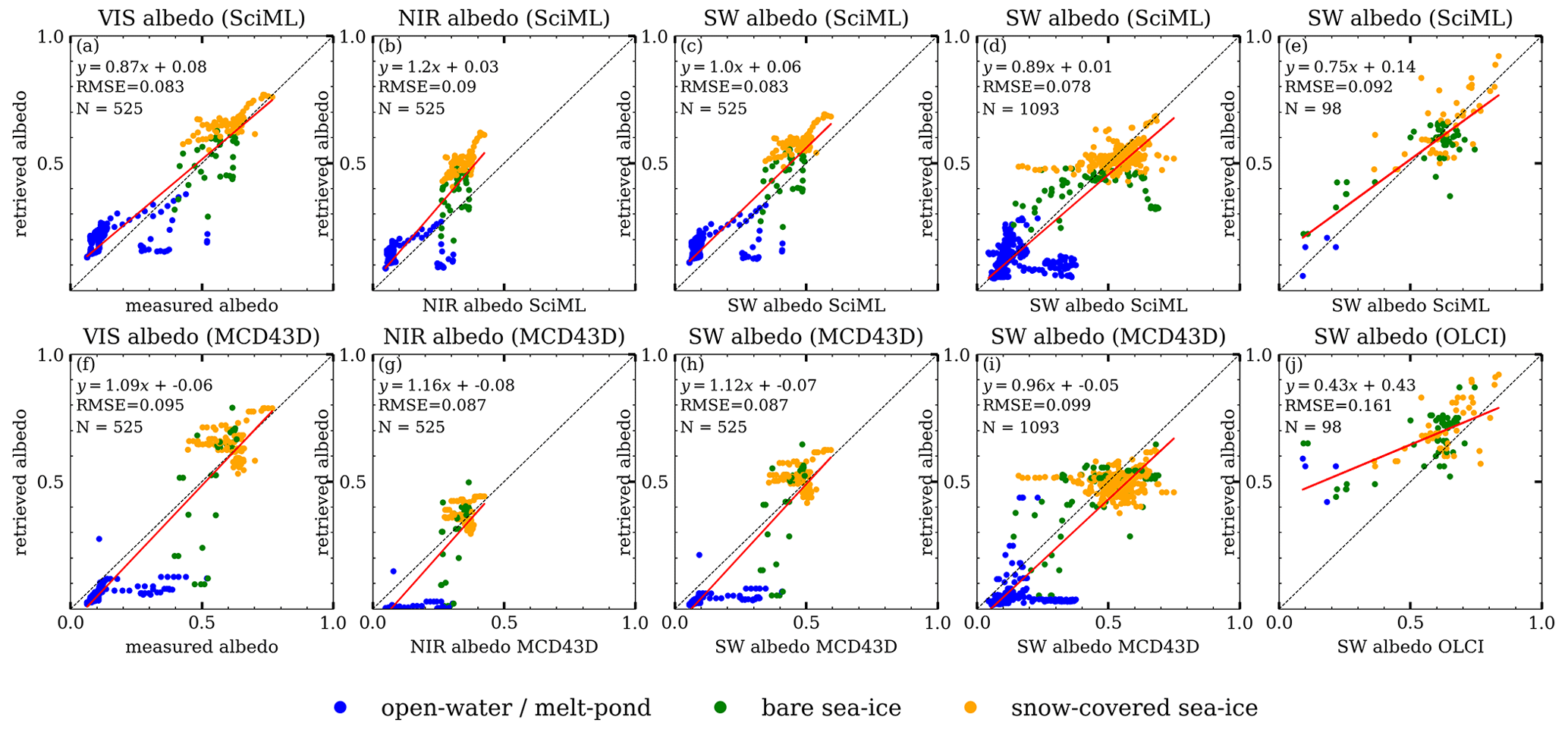
Figure 14 Correlation between satellite retrievals and ACLOUD albedo measurements utilizing three retrieval methods. (f–h) MCD43D albedo in the visible, near-infrared, and shortwave broadband compared to albedometer measurements; (i) MCD43D shortwave albedo compared to pyranometer measurements; and (j) comparison between the OLCI shortwave albedo derived with the MPD algorithm and all shortwave measurements from the ACLOUD campaign. (a–e) RTM–SciML retrievals that are regridded to the MCD43D or OLCI pixels. Surface type is represented by color. The regression relation between retrieval and measurements, RMSE, and the number of valid pixels are given in the upper left of each panel. Other statistical metrics (R², bias, f_EE≤15, etc.) can be found in Table B3 in Appendix B.

Because the BRDF is calculated using observations from a 16 d window, the MCD43 result cannot adequately capture daily albedo variations. One example is its failure to detect the opening of a melt pond north of Svalbard on 25 and 26 June, located at 80^∘ N, 15^∘ E. According to the eight RGB MODIS transit images (not shown), the melt pond began to open at 12:45 UTC on 25 June 2017, and by 15:05 UTC on 26 June 2017 the ice underlying the pond had entirely melted, leaving some bare sea ice (as categorized by the MLCM) surrounding the open water. While MCD43 could not identify this opening, the daily averaged RTM–SciML albedo indicates the snow and ice melting that resulted in the formation of a small open-water region.

Another point to emphasize is the lower albedo values obtained by MCD43 on snow-covered ice when compared to the RTM–SciML results, as demonstrated by the areas north and south of Nordaustlandet (near 80.5^∘ N, 22.5^∘ E and 78.5^∘ N, 25^∘ E, respectively). While there are no direct measurements to verify these values, we note that the underestimation of snow-covered area has been mentioned in several previous studies. For example, Stroeve et al. (2005) discovered that the MCD43 retrieval for snow-covered Greenland Ice Sheet (with an albedo greater than 0.7) has a −0.05 bias when compared to ground-based measurements. Similarly, An et al. (2020) observed underestimation when the albedo is greater than 0.4 for ice caps. For the particular case observed on these 2 d, the main reason is the extensive melting during the warm period (Knudsen et al., 2018).

Although the MCD43D V6.0 products have been adjusted to better capture shorter-term albedo variations through adjusting the BRDF weighting scheme to emphasize the BRDF of the day of interest inside the 16 d sliding window, by examining the quality product (i.e., MCD43A2), we found a much higher “BRDF albedo uncertainty” marked in the melting-snow areas as compared to the surrounding open water. According to Lucht and Lewis (2000), Wang et al. (2012), the uncertainty can be related to fluctuations in surface properties, atmospheric correction errors, high solar zenith angle (> 65^∘), and cloud detection during snow melt (among others). Figure 14 and Table B3 provide an approximation of the bias imparted by such uncertainty to sea ice albedo: compared to the “ground truths”, the MCD43D retrievals on open water and melt pond are significantly lower, and compared to the RTM–SciML retrievals at the same pixel the MCD43D snow retrievals are more dispersed.

5.2 Comparison with the MERIS-albedo product

Figure 15 compares the retrieval results obtained using the MERIS and RTM–SciML albedo retrieval algorithms during a 5 d period in 2007 between DOY 166 and 170. Additionally, the albedo values from CLARA-SAL product (Karlsson et al., 2012) and the melt pond fraction (Istomina et al., 2015) are given as a reference.

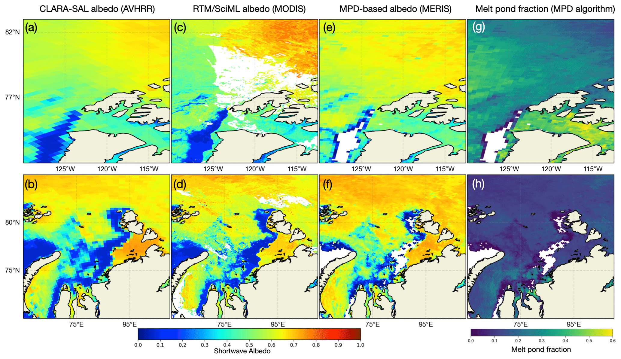
Figure 15 Maps of albedo and melt pond fraction averaged during a 5 d period in 2007 between DOY 166 and 170. From left to right, the columns show CLARA-SAL albedo, RTM–SciML-based albedo retrievals, MPD-based albedo retrievals, and the MPD-derived melt pond fraction (Karlsson et al., 2012 this study, and Istomina et al., 2015). The upper panels depict the Kara Sea, while the lower panels depict Banks, Prince Patrick, and Melville islands. At the bottom, color bars representing the corresponding values are displayed. In panels (c) and (d), empty regions represent cloud pixels that were detected by the MLCM cloud mask (and hence removed), whereas empty regions in panels (e) through (h) represent either cloud pixels or open-water areas that were not processed by the MPD algorithm.

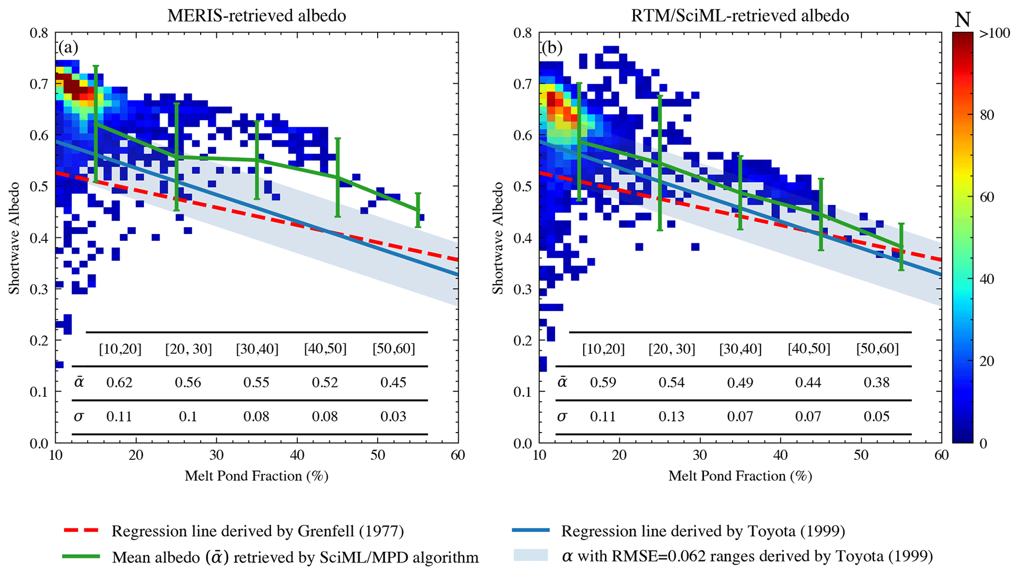
Figure 16 Density plot of the retrieved albedo in proportion to the melt pond fraction (f_mpf); values are derived from the regions depicted in Fig. 15. The color scheme represents number density. The inset table includes the mean ($\overline{\mathit{\alpha }}$) and standard deviation (σ) of albedo as retrieved by the SciML or MPD algorithm in different f_mpf intervals. The values are also represented by the green line in (a)–(b). The red lines represent the linear relation between f_mpf and sea ice albedo derived by Grenfell and Maykut (1977). The blue lines and shadings represent the f_mpf−α relation and the RMSE of 0.062 derived by Toyota et al. (1999).

The challenge of using the MPD algorithm to retrieve albedo is that the algorithm relies on certain empirically derived criteria (based on ratios of some radiance channels) to determine the exact type and composition of the corresponding pixel in order to assign an appropriate BRDF value for the valid or filling value for invalid observations. Since the assigned BRDF is used to derive albedo, the surface type was explicitly designated prior to albedo estimation. Moreover, the spectral reflection coefficients for the melt pond and thin ice boundaries, as well as the thick ice and snow cover boundaries, are manually adjusted based on the surface condition. Therefore, there are greater uncertainties in the retrieval during the transitional seasons of spring–summer and summer–autumn, as well as when the surface is highly heterogeneous (low sea ice concentration, discussed in Istomina et al., 2015); misclassification or improper manual assignment would result in a considerable uncertainty in the final albedo estimate.

As shown in Fig. 16, the two algorithms produce more consistent results for regions with low melt pond fraction, f_mpf, i.e., high sea ice concentration, f_sic; the average albedo values are similar when f_mpf≤30. However, the MERIS-derived albedo values in regions with large f_mpf values (f_mpf≥40 %) appear to be higher than those produced by the RTM–SciML model. Grenfell and Maykut (1977) derived a linear relation between f_mpf and the surface albedo (α), which is represented by the red lines in Fig. 16. Toyota et al. (1999) found a linear relation between ice concentration and albedo. In the absence of leads, the sea ice concentration and melt pond fraction has a $f_{\mathrm{sic}}+f_{\mathrm{mpf}}=\mathrm{1}$ relation. The shaded blue area and blue lines in Fig. 16 denote the f_mpf−α relation derived by Toyota et al.. Similarly, Petrich and Eicken (2009) reported reference albedo values of > 0.6 and < 0.5, respectively, for sea ice with 10 % and 50 % areal pond coverage. The sea ice albedo values produced by the RTM–SciML model correspond more closely to the reference values obtained by Toyota et al. (1999), Grenfell and Maykut (1977), and Petrich and Eicken (2009), whereas the values retrieved by the MPD algorithm are overestimated.

Another difference to note is the empty areas in Fig. 15. Chen et al. (2018) and Fan et al. (2021) demonstrated that the MLCM model we used for cloud filtering is more strict than the MODIS cloud filtering algorithm and is capable of identifying very thin cloud (and even fog; see Sect. 3) on bright surfaces such as snow and ice. The empty areas in Fig. 15c and d are MLCM-identified thin cloud pixels, whereas the empty areas in Fig. 15e through h represent open-water areas that were not processed by the MPD algorithm (Istomina et al., 2015).

5.3 Comparison with the OLCI-albedo product

Figure 17 depicts OLCI and RTM–SciML albedo retrievals on 24 and 26 June 2017. Additionally, broadband albedo values obtained using pyranometers Stapf et al. (2019) are displayed on top of the RGB images as reference.

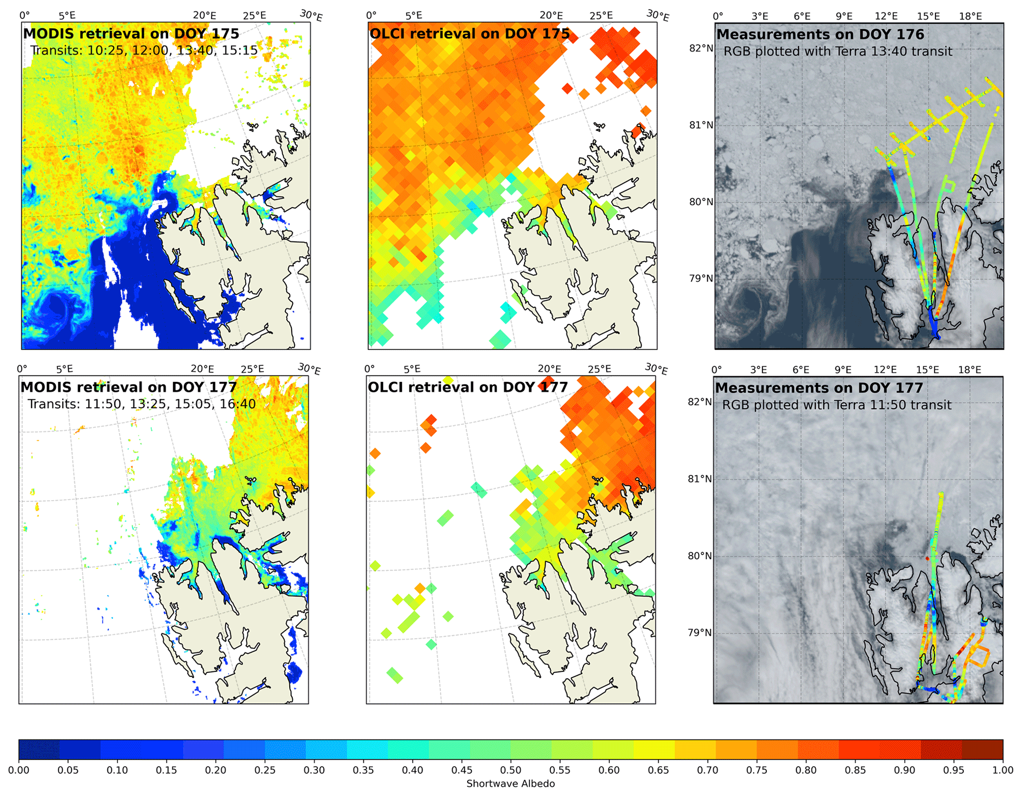
Figure 17 Maps of albedo derived using RTM–SciML (MODIS data) and the MPD algorithm (OLCI data, Istomina, 2020). The top panels depict albedo values on 24 June 2017, while the bottom panels depict values on 26 June 2017. From left to right, panels depict retrievals using RTM–SciML, MPD, and pyranometer measurements layered on an RGB image. On the associated images, the MODIS transits used to retrieve albedo and plot the RGB are labeled. Notably, no OLCI retrieval was available on 25 June 2017, and the campaign measurements for reference were taken on 25 and 26 June.

In the MPD algorithm, the type of ice used to calculate the ice-BRDF is referred to as “white ice” (Zege et al., 2015), which forms when meltwater drains intermittently from sea ice and has a few centimeters thick white coating that scatters light similarly to a thin snow layer (Grenfell and Warren, 1999; Tschudi et al., 2008).

Due to the logic of the underlying MPD algorithm, the OLCI and MERIS albedo products place a premium on the melt pond areas in the two polar regions. Because of the algorithm's emphasis on summer melting ice, it has various limitations, including being only applicable for data gathered from May to August, having a limited ability to retrieve albedo on snow-covered ice and ice with brine pockets inclusions, omitting retrieval for open-water areas, and having restrictions in areas with low sea ice concentration and very thin ponded ice.

When OLCI albedo maps are compared to in situ data (Fig. 17b–c), it is clear that the derived albedo values for snow-covered ice are excessively high (0.75 to 0.82 versus 0.65 to 0.7). On 26 June 2017 (DOY 177), the RGB image shows a few open-water spots around the northern coastline that are not captured by OLCI. This failure is partly attributable to the product's spatial resolution; data from its original resolutions (300 m at full resolution and 1.2 km at reduced resolution) were mapped to a 12.5 km NSIDC grid. However, the main reason is that the MPD employs pixels solely from sea ice grid cells and that open-water pixels have been filtered out using a brightness criterion. The error in the OLCI retrieval is quantified by the scatterplots in Fig. 14e–f and the statistics (R², RMSE, bias, etc.) in Table B3.

By comparison, the RTM–SciML albedo algorithm is capable of retaining the surface's albedo truthfully regardless of its condition and accurately reflecting the albedo values of these surfaces (i.e., more consistent with the measured albedo values). The current MLCM tool does not discriminate melt ponds from bare ice and labels both as “sea ice”. Because the MPD algorithm employs reflectance values from three visible channels (442, 490, and 510 nm), we may use a similar criterion to derive the melt pond fraction from MODIS or perhaps other sensors as well in the future.

5.4 Comparison with the direct-estimation algorithms (GLASS and VIIRS SURFALB)

At the time this paper was written, the phase-2 GLASS surface albedo product acquired using the MODIS sensor (Li et al., 2018) had not yet been released; the V40 GLASS (MODIS) product listed on the product page (http://www.glass.umd.edu/Download.html, last access: 18 February 2023) covers just land surface, leaving ocean surface blank. Consequently, the V40 GLASS (AVHRR) is compared to RTM–SciML retrievals in the following section.

The ACLOUD campaign was conducted during the 2017 spring-to-summer transition, which marked the beginning of the melt season, with snow-covered sea ice predominating and a small percentage of melt ponds. Three distinct synoptic weather periods were defined: a cold period (23–29 May 2017), a warm period (30 May to 12 June 2017), and a normal period (13–26 June 2017) (Wendisch et al., 2019; Knudsen et al., 2018). Throughout the cold period, surface conditions were relatively steady, with albedo values reaching 0.8 on snow-covered ice and approaching 0.6 on bare sea ice. During the warm period, the northwesterly wind pushed the Greenland coastal ice southward, resulting in the creation of the Northeast Water (NEW) Polynya and the opening of the region north of Nordaustlandet (Wendisch et al., 2019). It is evident from Fig. 18 that the RTM–SciML model accurately represents the three synoptic periods, including the emergence of NEW Polynya during the warm period and the polynya's closure during the normal period. In contrast, GLASS (AVHRR) is incapable of detecting these transitions.

In Fig. 10 of Qu et al. (2016), the CLARA SAL was used as a reference to compare albedo maps acquired from GLASS (MODIS) with comparisons performed in the same regions as depicted in Fig. 15 of this work. Comparing the two figures demonstrates that the RTM–SciML retrievals agree well with direct-estimation results. Therefore, the limitation of GLASS (AVHRR) could be attributable to the restricted number of shortwave channels accessible for the AVHRR sensor (three as opposed to seven for MODIS).

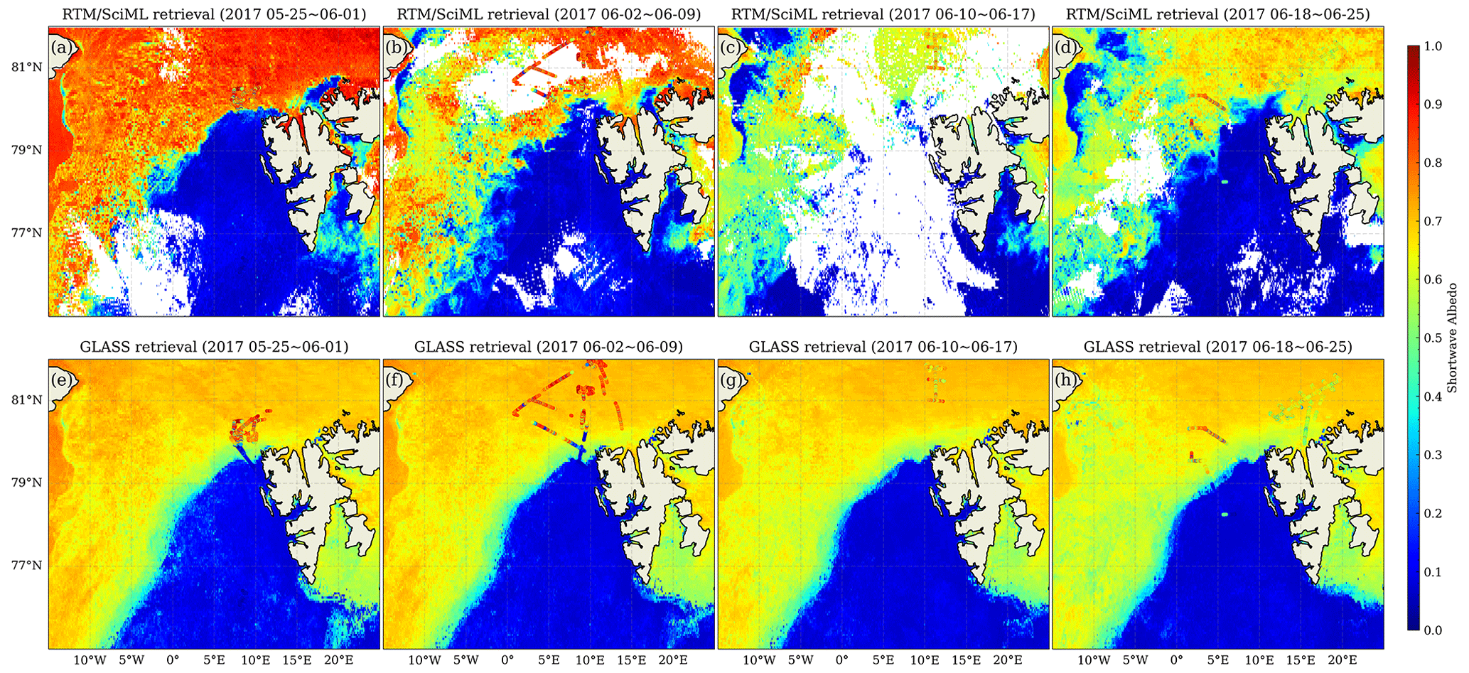
Figure 18 Maps of albedo derived using RTM–SciML (MODIS) and the direct-estimation algorithm (AVHRR data, Liang et al., 2021) averaged during 8 d periods. In the top row, empty regions represent areas obscured by cloud throughout the 8 d periods. The pyranometer measurements from the ACLOUD campaign are superimposed over the retrieval maps for the following flights: (a, e) the flight on 31 May 2017; (b, f) the flights on 2, 4, and 8 June 2017; (c, g) the flight on 14 June 2017; and (d, h) the flights on 18, 20, 25, and 26 June 2017.

Figure 19 shows pan-Arctic albedo images retrieved using RTM–SciML (MODIS and SGLI), the direct-estimation approach (VIIRS), and the MPD method (OLCI) for 2 representative days with thick ice (partially covered with snow) and melting ice. In order to facilitate analyses, Fig. 20 displays the longitudinally averaged albedo based on data collected on the same days. Because neither VIIRS nor OLCI provides open-water retrieval and the cloud-filtering data from the four sensors differ, data are collected to calculate an average only when all four albedo products (MODIS, SGLI, VIIRS, and OLCI) have values at the same grid cells. Moreover, Fig. B3 illustrates the percentage difference between each retrieval result and the CLARA-SAL product (Karlsson et al., 2020). The albedo estimated with MODIS and SGLI sensors using RTM–SciML models agrees quite well with the CLARA-SAL values. The VIIRS retrievals shown in the 29 June image are more comparable to these three, but the 15 July image appears to have lower values.

Due to the use of an uncoupled RTM in the training dataset for the direct-estimation method, the depths of snow, sea ice, and melt ponds were retained as fixed values, hence restricting the algorithm's retrieval precision for the more variable sea ice surfaces. The VIIRS SURFALB product relies on linear relations between TOA reflectance and surface albedo at various angular bins stored in a look-up table (LUT). The LUT include over 40 000 combinations of geometry angles. Multiplying the RTM-simulated or measured surface BRDFs (around 120 000) by the possible atmospheric configurations and by the geometry angle dataset, the resulting LUT is enormously large. Note, however, that only tens of thousands of surface situations were defined by the enormous LUT. Snow in nature possesses complex surface cover (which varies with density, impurity inclusions, thickness, and effective grain size), but the LUT employed in the VIIRS SURFALB product simply featured a snow layer with a fixed depth. The same issue exists in terms of sea ice conditions. In addition, since a LUT is essentially a linear regression model, the probable correlations between geometry angles and radiance or reflectance values from different channels are not learned in the training (i.e., look-up values from the table) process.

It is difficult to construct a quantitative comparison between the RTM–SciML albedo and VIIRS SURFALB products due to the lack of validation data that overlaps with the operational time of VIIRS SURFALB. Nonetheless, it is essential to highlight the value of our product's ability to retrieve albedo from any heterogeneous sea ice surface, given that the impurities, pond depths, snow cover, and ice layers are all included in the training data for RTM–SciML models.

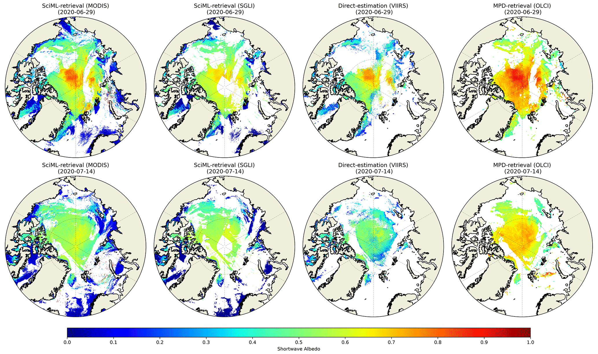
Figure 19 Pan-Arctic maps of albedo created using (from left to right) RTM–SciML (MODIS), RTM–SciML (SGLI), direct-estimation method (VIIRS), and MPD method (OLCI). The top row represents values for 29 June 2020, while the bottom row represents values for 14 July 2020. Empty regions in the SciML images represent cloud pixels that were detected by the MLCM cloud mask, whereas empty regions in VIIRS and OLCI images represent either cloud pixels or open-water areas that were not processed by the algorithms.

Figure 20 Longitudinally averaged albedo based on data from Fig. 19. Only when all four albedo products (MODIS, SGLI, VIIRS, and OLCI) have values at the same grid cells are data collected for the calculation of the longitudinal average. In addition, the average albedo of APP-x and CLARA-SAL (5 d temporal resolution, Karlsson et al., 2020) are displayed as points of reference. The temporal coverages of CLARA-SAL are (a) 25–29 June 2020 and (b) 15–19 July 2020.

6 Conclusion and summary

In this study, we described the development of a novel RTM–SciML sea ice albedo retrieval tool that can be applied to optical sensors that measure suitable radiance data. Comparisons of the retrieval results from SGLI and MODIS sensors with measurements showed good agreement. On a pan-Arctic scale, retrieval results derived from RTM–SciML models are most similar to the CLARA-SAL values, suggesting the reliability of the RTM–SciML framework. For in situ validation, comparison with albedo values acquired during low-level aircraft flights and retrieval of albedo values based on more than 2000 data points during cloudless conditions demonstrated a small RMSE of 0.066.

The RTM–SciML albedo algorithm was trained on a large synthetic dataset generated using a coupled RTM and represents the optical properties of the cryosphere surface (bare ice, snow-covered ice, water, and melt pond). The combination of these two characteristics enables it to exploit the advantages of both the AccuRT and the RTM–SciML simulation tools.

When building the SD, we can reap the benefit of AccuRT being a RTM for the coupled system that accurately incorporates atmosphere–snow–sea ice–water interactions to compute TOA radiances and corresponding surface albedo values. Information of both the surface BRDF and the IOPs of the atmosphere is implicitly taken into account. We are thus saved from the procedure to perform atmospheric corrections. This retrieval procedure does not rely on predefined spectral reflectance threshold values for individual types of surface; the surface classification and albedo retrieval are separate processes, which eliminates errors caused by incorrect surface condition assumptions.

The RTM–SciML albedo algorithm still possesses certain limitations. Without prior knowledge of the underlying radiative transfer theory, the ML models addressed in this paper can only approximate the hard-limit physical model (a RTM). Therefore, there may be adversarial instances in which small perturbations in the input data result in drastically divergent retrieval outcomes. Creating specialized network architectures and tailoring loss functions that represent known physical systems is one method for tackling this under-specification challenge (i.e., physics-informed neural networks, PINNs, Cuomo et al., 2022; Daw et al., 2021; Di Natale et al., 2022).

Meanwhile, in the current training data, snow or ice does not exhibit layered topographic variation for the sake of simplicity. Additionally, the present RTM–SciML albedo retrieval tool does not account for whitecaps and sun glints on the open-ocean surface that would occur at oblique viewing angles. Nevertheless, the limits regarding training data can be adequately addressed by extending the SD in accordance with pertinent RTM simulations.

In summary, the RTM–SciML framework presented and discussed here has huge potential for the following reasons.

1. It may be used to retrieve albedo of relatively flat glaciers because a flat layer of glacier ice is similar to sea ice without brine pockets (Warren, 2019). The “wind-roughened air–water interface” can be represented in AccuRT using a one- or two-dimensional Gaussian surface slope distribution (for details, see Stamnes et al., 2018). In comparison to the existing method for retrieving glacier albedo (Ren et al., 2021), which uses the measured BRDF of sea ice to approximate glacier-BRDF (Gatebe and King, 2016) and bi-conical band reflectance observed by a spaceborne imaging radiometer to approximate the ice albedo in the shortwave-infrared band, the methodology we propose here may be more appropriate for characterizing the anisotropic reflectance of a rough glacier surface.

2. The framework is generic in nature, allowing for comparisons between not only the MODIS sensors mounted on Terra and Aqua but also a large number of existing polar-orbiting sensors and well-planned future sensors, enabling sensor-to-sensor retrieval comparisons. In a recent review, Liang et al. (2019) emphasized the importance of developing retrieval algorithms that are broadly applicable to all satellite sensors: albedo retrievals based on multi-platform satellite sensors can significantly increase the amount of valid and accurate observational data, thereby increasing spatial and temporal coverage regardless of the specific method of retrieval. Meanwhile, developing retrieval algorithms using the same methodology enables a more extensive examination of the uncertainty associated with each sensor (e.g., identifying saturated channels and developing uncertainty assessment methods). The RTM–SciML framework presented in this paper is ideally suited for such a requirement.

Appendix A: Parameterizations in the synthetic dataset (SD) for coupled RTM as input

A1 Bare sea ice

The radiative transfer processes in bare sea ice include absorption by pure ice, scattering by air bubbles, and scattering and absorption by brine pockets and solid salts (Jin et al., 1994). Unfortunately, direct observational data of air bubble volume fraction and radius (V_bu, r_bu) in the field is difficult (Petrich and Eicken, 2009). Lindsay (2001) used sea ice thickness as the main factor to parameterize areal albedo and achieved an uncertainty within 0.05 and 0.10 (even without cloud screening), showing that sea ice thickness is the dominant parameter determining bare sea ice albedo.

Table A1 Physical parameters of ice. In generating the sea ice thickness, a truncated-normal distribution (μ=0.03; σ=1.5) was used to ensure an adequate amount of thin ice in the SD. The brine pocket radius conforms to a Tukey lambda distribution (with λ=0.5).

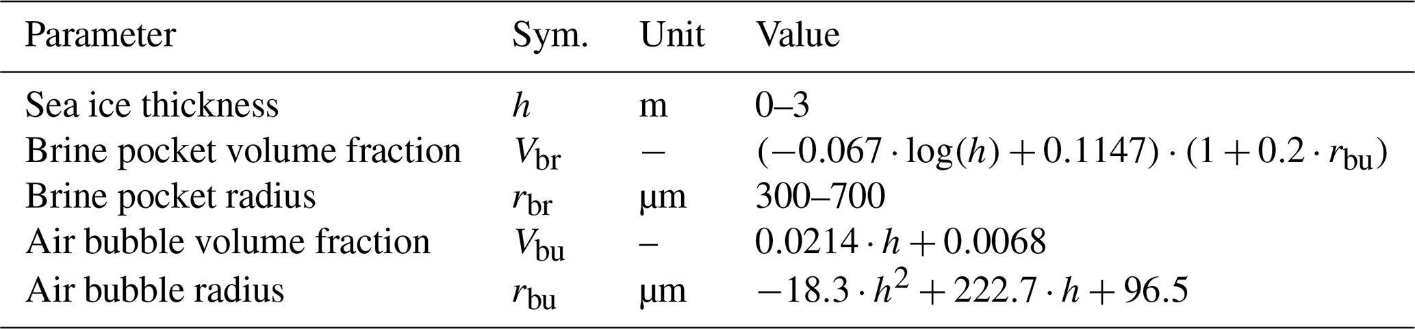
For the parameterization of sea ice in this study, the rest of the sea ice parameters (including brine pocket volume fraction, air bubble volume fraction, air bubble radius) are linearly fitted as a function of sea ice thickness (h) as shown in Table A1. The expectations are that thinner new young ice (NYI) and first-year ice (FYI) (≤ 30 cm and ≤ 1 m) would contain fewer bubbles and would in general be more saline than the thicker, multi-year ice (MYI) counterpart (≥ 1.5 m). As sea ice deteriorates, brine water is excluded in the desalination process, which results in a smaller brine pocket volume fraction and radius values (V_br, r_br). Empirical equations were derived with the typical values of bubble and brine parameters for sea ice with increased thickness (adopted from Table 1 in Stamnes et al., 2011).

It is worth noting that the equation of bulk brine concentration with ice thickness in Toyota et al. (2007) (which is based on in situ measurements of sea ice from the Sea of Okhotsk) and our equation (V_br in Table A1) both show brine concentration approaching ∼10 % asymptotically as sea ice thickens.

A2 Sea ice covered with meltwater

The water depth on thinner ice is in general shallower than on thicker ice. This situation is particularly true for the coastal polynya region, where ice intermittently melts and refreezes from meltwater. In addition to temperature, the topography of the ice underneath also influences meltwater depth. A thinner ice layer is unlikely to evolve into hummocky topography (like MYI ice surfaces) to hold deep meltwater (Perovich and Polashenski, 2012).

Generally, melt ponds on sea ice do not exceed 1 m thickness. From RTM simulations, we found that a pond thickness of 1.5 m was the critical value that distinguishes the sea ice properties from the overlying meltwater, and we therefore use it as the upper limit of meltwater thickness (Table A2).

In order to increase the variation in the SD, in addition to the meltwater in the first ocean layer, we also added variation to the chlorophyll a (chl a) concentration as well as colored dissolved organic matter (CDOM) concentrations in the third ocean layer (the second layer is sea ice) in ranges typical for the areas with sea ice cover (König et al., 2019; Mustapha and Saitoh, 2008).

Table A2 Physical parameters of meltwater on ice and ocean water. Meltwater thickness and CDOM values follow randomly distributed uniform distributions in the specified ranges. For the chl a concentration, a reciprocal continuous distribution (long tail extending to high values) was used.

A3 Sea ice covered with snow

The albedo of snow depends on the grain shape and size, solar zenith angle, impurities in the snow, surface roughness, the thickness of the snow layer (Grenfell et al., 1994), and the sky condition (clear or cloudy).

The snow cover on all sea ice types can accumulate to optically thick values (> 10 cm). Nihashi et al. (2009) found that with snow present a 16 cm snow layer on 80 cm thick first-year ice would have the same insulation effect as a much thicker, 192 cm slab of ice. Similarly, in their simulations, Hamre et al. (2004) found that 2.5 cm thick snow cover has about the same transmittance as a 61 cm thick ice layer. In our simulations, the spectral albedo of both coarse-grained (700 µm) and fine-grained (100 µm) pure snow (impurity fraction $f_{\mathrm{imp}}={\mathrm{10}}^{-\mathrm{8}}$ ) both saturate when the thickness approaches 20 cm; beyond this limit, adding more snow does not further increase the albedo. This value is therefore set as the upper boundary of snow cover depth.

In their snow grain size retrievals, Jäkel et al. (2021a) found an optically equivalent snow grain size (r_e) on glacier and smooth land surfaces centered in the 50–100 µm range, while the range on smooth sea ice surfaces was 100–150 µm. A broad range of 50–150 µm was adopted in our SD simulations (Table A3).

Table A3 Physical parameters of snow cover. The snow grain size and snow thickness were generated with a randomly uniform distribution in the specified ranges.

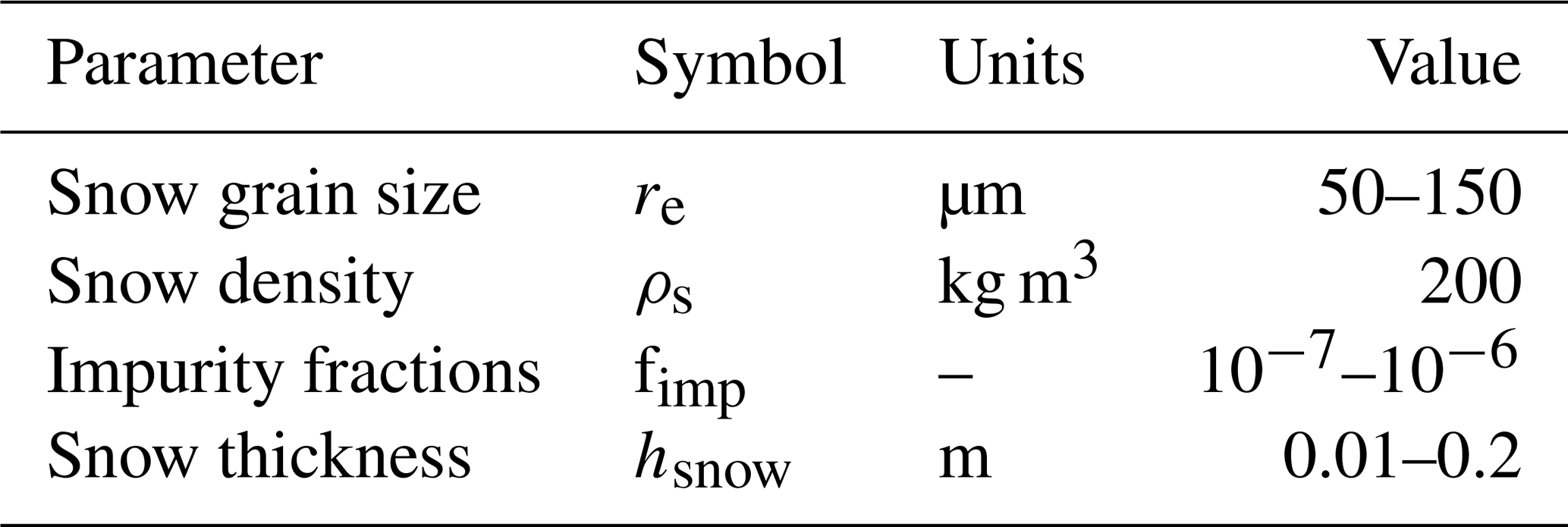
A4 Geometries and atmospheric parameters

The temperature, pressure, and concentrations of the major atmospheric elements were described using the “subarctic summer” atmospheric profile (Anderson et al., 1986). The small amount of aerosols typically found in the sea ice regions on cloud-free days and the relative impact of aerosols on the surface reflectance of such a bright surface indicate that the aerosol optical depth (AOD) shown in Table A4 will suffice (Mehta et al., 2016; Winker et al., 2013).

Table A4 Geometries and atmospheric parameters. All parameters conform to random uniform distributions in the specified ranges.

Appendix B: Appendix figures and tables in discussion

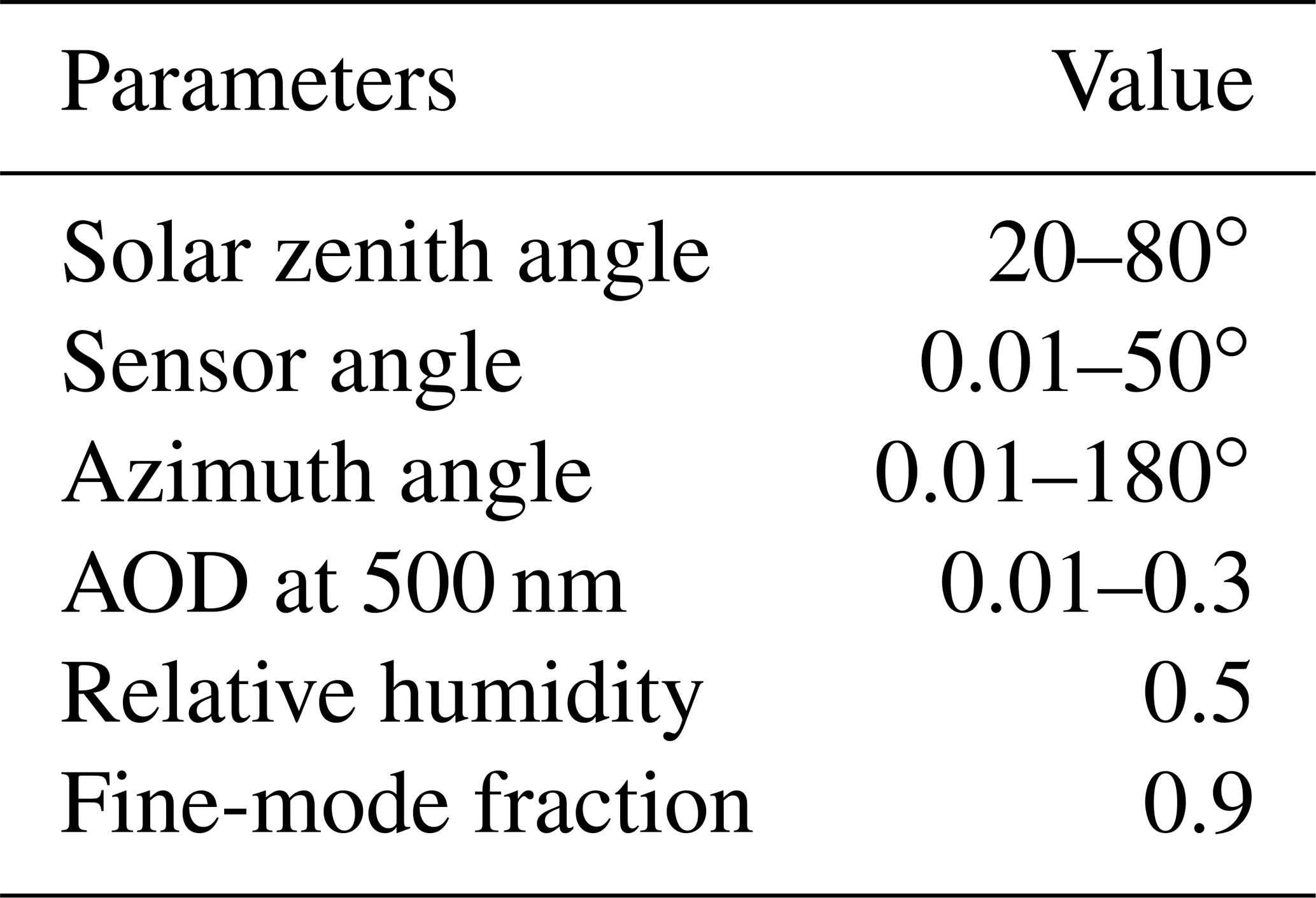
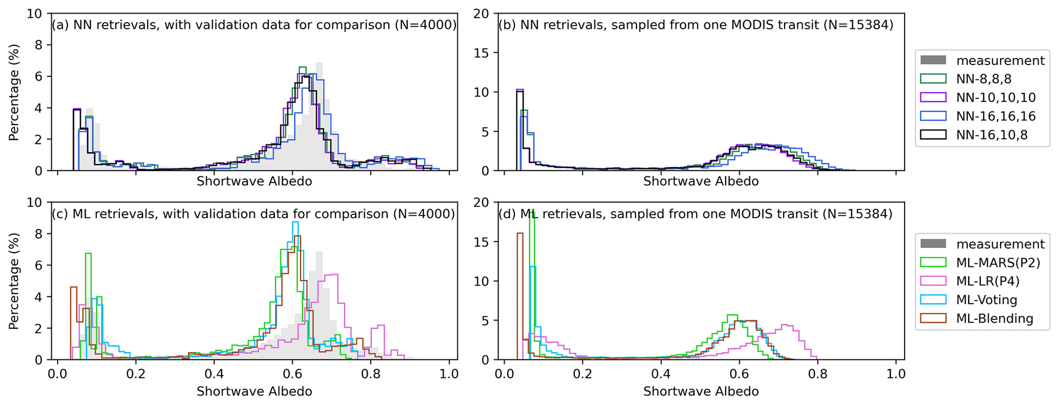
Figure B1 The top and bottom rows show a comparison of the retrieval results from four MLANN models and four ML models, respectively. The validation results of the eight selected models against aircraft measurements are provided in Table B1. Histograms of the measurements are presented as a reference (gray areas) in (a) and (c). Panels (b) and (d) are sampled retrieval results using data from the MODIS transit at 14:00 UTC on 25 June 2017.

Table B1 Summary of the evaluation results using pyranometer data sampled from Sect. 2.5.2 (N=4000). The SciML models were classified into seven categories: linear regression with polynomial terms, multivariate adaptive regression splines (MARS) with polynomial terms, principal component analysis (PCA)-processed MARS, tree models, voting ensembles, linear blending ensembles, and MLANN. Within each category, the models that perform the best are shown in bold. The following metrics are used for evaluation: : R² score, Pearson r coefficient (r), RMSE, MAE, mean absolute percentage error (MAPE), f_above, f_EE≤15, f_below, and bias.

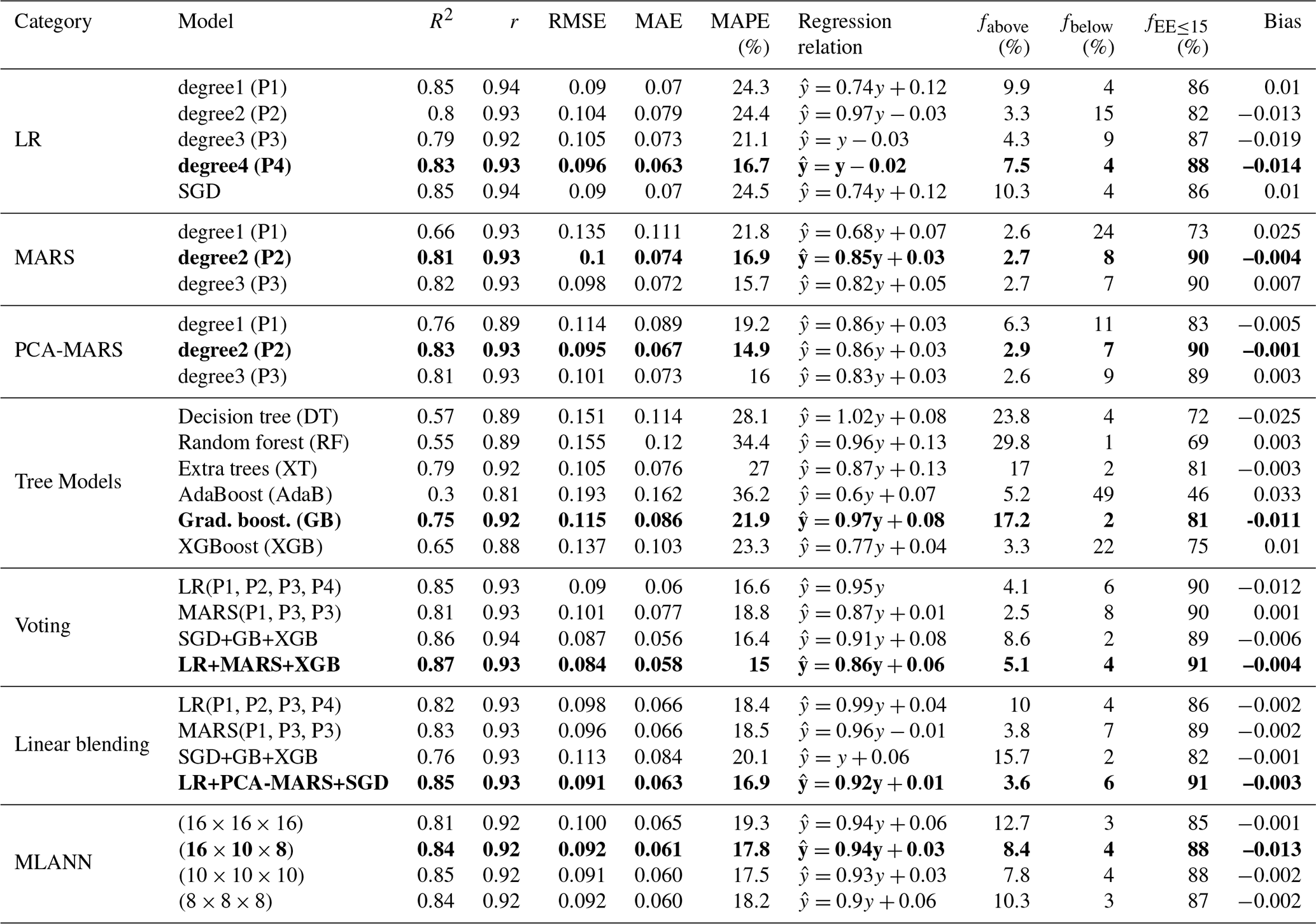
Table B2 Summary of the evaluation results for a time constraint with a loose value (δ_t≤5 h). The data were divided into four categories: three broadband albedos determined by the albedometer's spectral range and a single broadband shortwave albedo determined by the pyranometer's range. Three subcategories have been identified within each category: snow-covered sea ice (abbreviated as “snow” in the table), bare sea ice (“ice”), and open water (“water”). Pearson r coefficient (r), root-mean-square error (RMSE), mean absolute error (MAE), mean absolute percentage error (MAPE), f_above, f_EE≤15, f_below, and bias are used to evaluate the retrieval in the subcategories (snow, ice, and water) and the total valid data (“all”). On the right side of the table, the total number of data in each subgroup is included (N).

Figure B2 The same as Fig. 4 but with the surface type represented by color. In addition, the lower-right corner of each panel displays data for each surface type (r, RMSE, f_EE≤15, and N).

Table B3 Summary of the evaluation results for MCD43D and OLCI. The data were divided into four categories: three broadband albedos determined by the albedometer's spectral range and a single broadband shortwave albedo determined by the pyranometer's range. RTM–SciML retrievals have been regridded to compare the validation errors. R-squared values (R²), Pearson r coefficient (r), root-mean-square error (RMSE), mean absolute error (MAE), f_above, f_EE≤15, f_below, and bias are used to evaluate the retrieval in the subcategories (snow, ice, and water) and the total valid data (“all”). On the left side of the table, the total number of data in each subgroup is included (N).

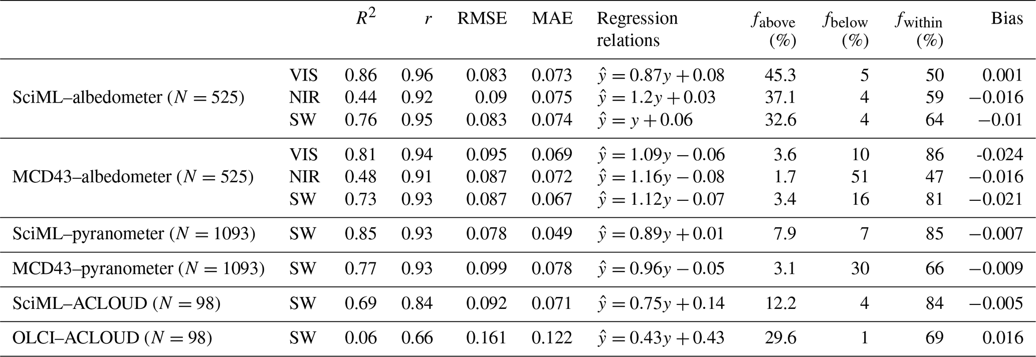
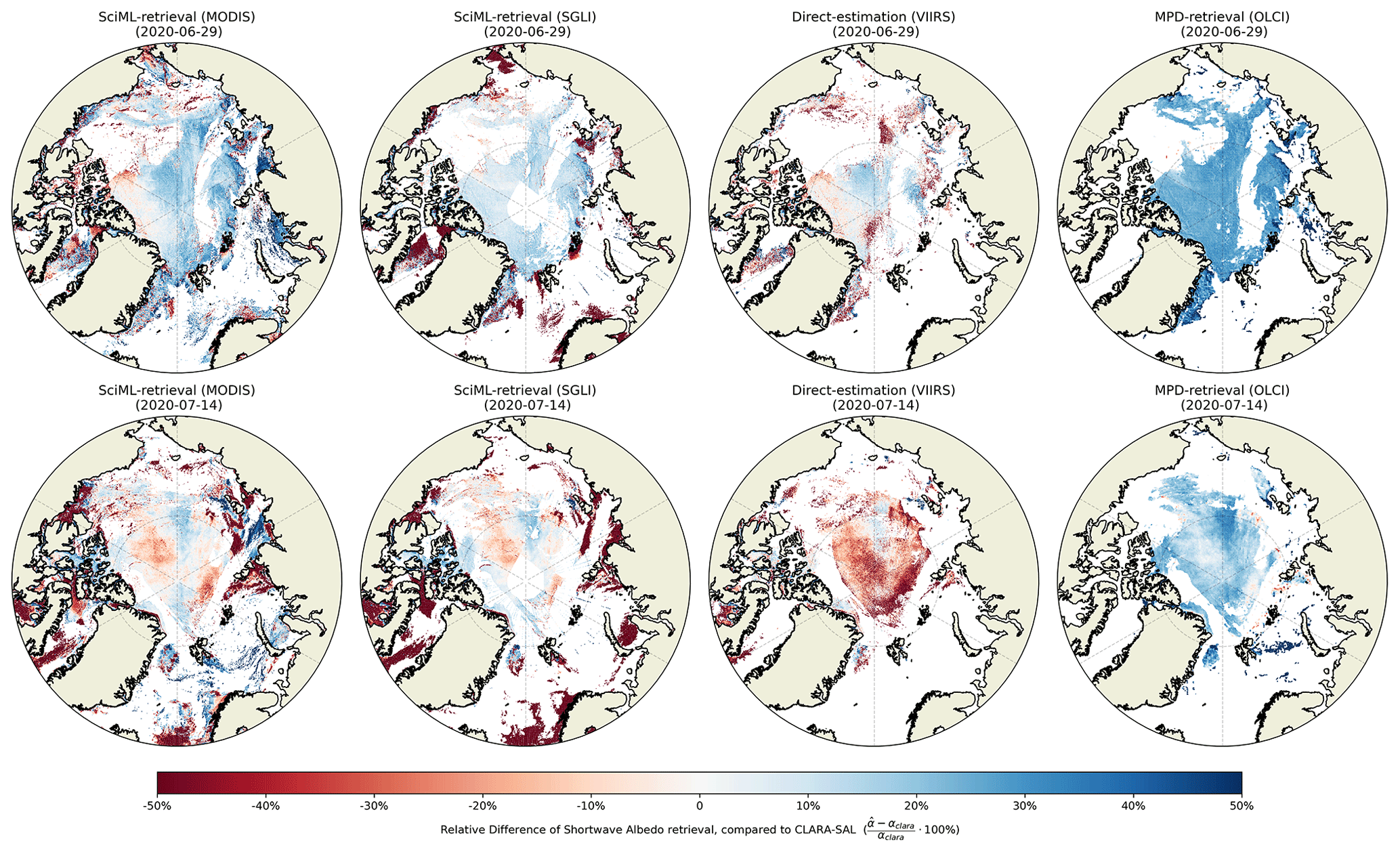
Figure B3 Percentage difference $({\displaystyle \frac{\widehat{\mathit{\alpha }}-{\mathit{\alpha }}_{\mathrm{clara}}}{{\mathit{\alpha }}_{\mathrm{clara}}}}\cdot \mathrm{100}\mathit{\%})$ in albedo maps as compared to the CLARA-SAL (Karlsson et al., 2020) results (from left to right): RTM–SciML (MODIS), RTM–SciML (SGLI), direct estimation (VIIRS), and MPD (OLCI). The top row represents values for 29 June 2020, while the bottom row represents values for 14 July 2020. Empty regions in SciML images represent cloud pixels that were detected by the MLCM cloud mask, whereas empty regions in VIIRS and OLCI images represent either cloud pixels or open-water areas that were not processed by the algorithms.

Appendix C: List of acronyms

AANN	Auto-associative neural network
ACLOUD	Arctic Cloud Observations Using Airborne Measurements During Polar Day
AFLUX	Airborne measurements of radiative and turbulent FLUXes of energy and momentum in the Arctic boundary layer
AVHRR	Advanced Very High Resolution Radiometer
BRDF	Bi-directional reflectance distribution function
BSA	Black-sky albedo
fbc	Black carbon impurity fractions
fcloud	Cloud fraction
fEE≤15	Percentage of data within 15 % expected error
fmpf	Melt pond fraction
fsic	Sea ice concentration
GLASS	Global Land Surface Satellite
IOPs	Inherent optical properties
MAPE	Mean absolute percentage error
MERIS	MEdium Resolution Imaging Spectrometer
MISR	Multi-angle Imaging SpectroRadiometer
MLCM	Machine Learning Classification Mask
MLANN	Multi-layer artificial neural network
MODIS	Moderate Resolution Imaging Spectroradiometer
MOSAiC	Multidisciplinary drifting Observatory for the Study of Arctic Climate
MPD	Melt pond detection
NIR	Near infrared
NTBC	Narrow-to-broadband conversion
OLCI	Ocean and Land Colour Instrument
PDF	Probability density functions
SciML	Scientific machine learning
SD	Synthetic dataset
SGLI	Second-generation Global Imager
SMART	Spectral Modular Airborne Radiation measurement system
STBC	Spectral-to-broadband conversion
SURFALB	Surface albedo (the SURFALB product of VIIRS)
SW	Shortwave
TOA	Top of the atmosphere
VIS	Visible
VIIRS	Visible Infrared Imaging Radiometer Suite