Characterizing tundra snow sub-pixel variability to improve brightness temperature estimation in satellite SWE retrievals

Topography and vegetation play a major role in sub-pixel variability of Arctic snowpack properties but are not considered in current passive microwave (PMW) satellite SWE retrievals. Simulation of sub-pixel variability of snow properties is also problematic when downscaling snow and climate models. In this study, we simplified observed variability of snowpack properties (depth, density, microstructure) in a two-layer model with mean values and distributions of two multi-year tundra dataset so they could be incorporated in SWE retrieval schemes. Spatial variation of snow depth was parameterized by a log-normal distribution with mean (μ_sd) values and coefficients of variation (CV_sd). Snow depth variability (CV_sd) was found to increase as a function of the area measured by a remotely piloted aircraft system (RPAS). Distributions of snow specific surface area (SSA) and density were found for the wind slab (WS) and depth hoar (DH) layers. The mean depth hoar fraction (DHF) was found to be higher in Trail Valley Creek (TVC) than in Cambridge Bay (CB), where TVC is at a lower latitude with a subarctic shrub tundra compared to CB, which is a graminoid tundra. DHFs were fitted with a Gaussian process and predicted from snow depth. Simulations of brightness temperatures using the Snow Microwave Radiative Transfer (SMRT) model incorporating snow depth and DHF variation were evaluated with measurements from the Special Sensor Microwave/Imager and Sounder (SSMIS) sensor. Variation in snow depth (CV_sd) is proposed as an effective parameter to account for sub-pixel variability in PMW emission, improving simulation by 8 K. SMRT simulations using a CV_sd of 0.9 best matched CV_sd observations from spatial datasets for areas > 3 km², which is comparable to the 3.125 km pixel size of the Equal-Area Scalable Earth (EASE)-Grid 2.0 enhanced resolution at 37 GHz.

1 Introduction

Snow cover is known to be highly variable at the local scale (10–1000 m) due to wind redistribution, sublimation (Liston and Sturm, 1998; Winstral et al., 2013) and vegetation trapping (Sturm et al., 2001). Physical properties of snow such as measurement of stratigraphy (Fierz et al., 2009) can be aggregated into layers, but their spatial distribution is highly variable given their dependence on total depth and surface roughness (Liljedahl et al., 2016; Rutter et al., 2014). Such variability leads to uncertainties in the retrievals of snow state variables such as snow water equivalent (SWE) using microwave remote sensing from local scales (King et al., 2018; Rutter et al., 2019) to global scales (Pulliainen et al., 2020). Improving our empirical understanding of the processes governing this variability would improve spaceborne snow monitoring, especially in Arctic regions where ground measurements and weather station networks are sparse.

Measurement of SWE using passive microwave satellite data (Larue et al., 2018; Pulliainen, 2006) is possible using a radiative transfer model to simulate snow emission at various frequencies, from which an inversion of the model can produce global estimates of snow depth (Takala et al., 2011). More specifically, passive microwave brightness temperatures (T_B) are governed by radiometric properties of the layered snowpack. As such, each layer has its own absorption and scattering properties; the amount of scattering is proportional to snow total mass where the scattering and emission is frequency-dependent (Kelly et al., 2003). Scattering at higher frequencies such as 37 GHz, will lead to lower T_B, so differences between T_B at two frequencies (37–19 GHz) are related to snow mass (Chang et al., 1982). Arctic snowpack mainly consists of two distinct layers (wind slab and depth hoar), where each layer has unique scattering properties (Derksen et al., 2010). Complexity of the layered properties (density, temperature and microstructure) strongly influences radiative transfer modeling (King et al., 2015; Rutter et al., 2014). Furthermore, recent developments in radiative transfer modeling (SMRT: Picard et al., 2018; DMRT: Tsang et al., 2000; and MEMLS: Wiesmann and Mätzler, 1999), microstructure representation (Royer et al., 2017) and in situ measurement of snowpack properties (Gallet et al., 2009; Montpetit et al., 2012; Proksch et al., 2015) have provided significant agreement between models and in situ measurements. However, spatial distribution and heterogeneity of total snow depth and stratigraphy remain challenging to implement and are not considered for large-scale monitoring of SWE in tundra environments. Rutter et al. (2019) and Saberi et al. (2020), using three- and two-layer models respectively, demonstrated a relationship between the ratio of depth hoar and wind slab with respect to total depth, enabling the usage of the proportion of these two layers with total snow depth. Working with a simplified layer representation of a snowpack with well-defined physical properties may adequately characterize snowpack for large-scale SWE retrievals.

Two dominant processes governing snow depth variability in the Arctic are (1) wind redistribution with topography (Sturm and Wagner, 2010; Winstral et al., 2002) and (2) vegetation trapping (Domine et al., 2018; Sturm et al., 2001). Liston (2004) described snow depth heterogeneity using a log-normal distribution with a coefficient of variation of snow depth (CV_sd), the ratio between standard deviation (σ_sd) and the mean of snow depth (μ_sd), indicating the extent and spread of a distribution (i.e., high variability over thin snow will lead to high values of CV_sd). Also, Liston (2004) proposed nine categories of CV_sd with values ranging from 0.9 to 0.06 for midlatitude treeless mountains to ephemeral snow, where arctic tundra type was 0.4. Snow depth variability is based on a parametrization of μ_sd and CV_sd on the log-normal distribution scale parameters (λ, ζ). Gisnås et al. (2016) adapted that approach using scale parameters (α, β) of the gamma distribution. In all cases, CV_sd is used to describe sub-grid variability (Clark et al., 2011), but its value remains challenging to quantify given that regional trends are linked to topography, vegetation and climate (Winstral and Marks, 2014). In this context, CV_sd is used to quantify spatial heterogeneity of snow in climate modeling but so far has not been used in microwave SWE retrievals.

In SWE retrievals, snow depth is assumed to be uniform, and the mean depth is used to optimize brightness temperature and derive SWE from depth and assumed density (Kelly, 2009). There is potential for CV_sd to be used as an effective parameter to estimate sub-pixel variability in brightness temperature. Bayesian frameworks are used in inversion schemes for SWE retrievals (Durand and Liu, 2012; Pan et al., 2017; Saberi et al., 2020) using a priori information (density, microstructure and temperature) from regional snowpack characteristics and inversion of radiative transfer models (Saberi et al., 2020). An iterative approach based on Bayesian theory is used (Takala et al., 2011) to match observed brightness temperature with modeled brightness temperature by iterating a priori information of the snowpack in order to derive snow depth and SWE. Saberi et al. (2020) conducted a case study for snow depth retrievals using a two-layer model from airborne microwave observations using a Bayesian framework (or Markov chain Monte Carlo) over tundra snow. However, high uncertainty (21.8 cm) in retrieved snow depth (via T_B) resulted, which suggested the use of a term involving variation in snow depth and microstructure within the footprint instead of a uniform snow depth.

To address this research gap, we used a multi-year snow dataset from two Arctic locations to quantify sub-pixel variability of snow depth and microstructure and used CV_sd as an effective parameter that controls snow sub-pixel variability. Firstly, we evaluate tundra snow depth spatial variability using probability density functions (log-normal and gamma) and its parameters, μ_sd and CV_sd. Secondly, we present from in situ observations distinct snow microstructure and density values of both tundra main layers (depth hoar and wind slab), mean ratios of layer thickness, and the depth hoar fraction (DHF) relative to snow depth. Finally, we perform a Gaussian process fit to estimate DHF from snow depth and used probability density functions of snow depth to add variation of snow depth and microstructure within the footprint. Then we compare mean pixel snow properties simulations with simulations of sub-pixel variation in snow properties to evaluate biases between measured T_B from a satellite sensor at 19 and 37 GHz and T_B simulated by inversion of a radiative transfer model.

2 Methods

2.1 Study site

Data were collected in two regions of the Canadian Arctic, with different topography and vegetation yielding different snow depth distributions. Trail Valley Creek (TVC) research watershed, Northwest Territories (68^∘44^′ N, 133^∘33^′ W), located at the southern edge of arctic shrub tundra, is dominated by herbaceous tundra and dwarf shrubs and characterized by gently rolling hills with steep slopes. Greiner Lake watershed, Cambridge Bay (CB), Nunavut (69^∘13^′ N, 104^∘53^′ W), located within arctic tundra, is characterized by dwarf shrub and calcareous tills on upland sites with gently rolling hills and small ponds and lakes. TVC is considered to have more subarctic attributes with predominant vegetation than CB given its proximity to the northern edge of the boreal forest. Topographic maps (Fig. 1; ArcticDEM) show slightly higher variation in elevation at TVC with plateau and steep slopes compared to CB, which is dominated by ponds and small variation in topography.

Figure 1 Locations of study areas in the Canadian Arctic, Cambridge Bay and Trail Valley Creek site. Grid shown is the enhanced 3.125 km EASE-Grid 2.0 (Brodzik et al., 2018) used for satellite data. The ArcticDEM used to show elevation has a 2 m resolution (Porter et al., 2018) derived from stereo high-resolution visible imagery for the entire Arctic domain, which is freely available.

2.2 Data

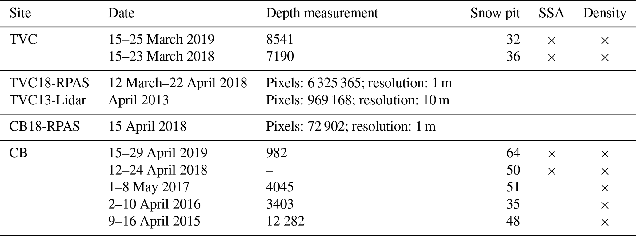
Snow pits (315) at each site (TVC: 68, CB: 248) provided information on snow layering, vertical profiles of geophysical properties (includes temperature, grain type classification, hardness, density, microstructure and depth). Measurements of visual stratigraphy and grain type classification were conducted following Fierz et al. (2009). Density was measured using 100 cm³ density cutters and digital scales. Snow specific surface area (SSA) was measured using an InfraRed Integrating Sphere (IRIS) (Montpetit et al., 2012) in Cambridge Bay and an A2 Photonic Sensors IceCube in TVC, both based on 1300 nm laser reflectometry (Gallet et al., 2009). Snow depth measurements, linear transects and circular transect around snow pits used a magnaprobe from SnowHydro LLC (Sturm and Holmgren, 2018), which is equipped with a standard GPS unit. Measured snow depth distributions were used to identify subsequent pit locations (on site) from a predefined transect across CB watershed in order to ensure the snow pit locations were representative of wider spatial variability (Table 1). For TVC, pit locations were chosen based on previous snow depth distribution (2016), slope and elevation. Multiple snow depth maps at 1 m resolution from remotely piloted aircraft system (RPAS) surveys derived from photogrammetry conducted in March 2018 (Walker et al., 2020a) were used to estimate snow depth distribution in TVC with total spatial coverage of 5.3 km². An airborne lidar dataset of TVC snow depths (93 km² at 10 m resolution) collected by an aircraft in April 2013 (Rutter et al., 2019) was also used. Monte Carlo simulations of both the μ_sd and CV_sd were performed on each snow depth map. Simulations randomly selected pixels as the center of a circular mask with a random radius. The mask was used to select all pixels within the circle so the statistical parameters (μ_sd and CV_sd) could be calculated. Also, a small RPAS map was available for CB with spatial coverage of 0.2 km² at 1 m resolution. Maps of normalized difference vegetation index (NDVI) were created from Sentinel-2 (10 m resolution) images from late summer (1 September 2019 for TVC and 8 September 2019 for CB).

Table 1 Summary of the number of snow depth measurements (magnaprobe and RPAS) and snow pit sites per year. The availability of SSA and density measurements across sites and years is also noted (×). See Table 2 for full dates.

2.3 Measured brightness temperatures and Snow Microwave Radiative Transfer (SMRT)

Microwave T_B values were used to evaluate simulations from SMRT at 37 and 19 GHz from the Special Sensor Microwave/Imager and Sounder (SSMIS) sensor, with the Equal-Area Scalable Earth (EASE)-Grid 2.0 resampled at 3.125 km (6.25 km for 19 GHz) resolution (Brodzik et al., 2018), for both TVC and CB regions. T_B values were estimated by averaging all pixels within snow pit area (CB: 24 pixels, TVC: 8 pixels for 37 GHz). Each pixel with at least one snow pit inside was used. Since all snow pits were aggregated to obtain mean value and distribution of snow properties for SMRT, averaged T_B covering the snow pits area was used.

The area was also filtered to remove any contribution from sea or deep lakes, as pixels with liquid water exhibit large biases even if the signal at 37 GHz is mostly sensitive to snow (Derksen et al., 2012). For CB, an area with the same spatial coverage but a slightly different location was used since the snow pit area was within 25 km (full resolution of SSMIS) from the ocean. T_B values were temporally averaged to match times of field measurements, representing peak winter snow accumulation (Table 2). Also, T_B values were corrected for atmospheric contributions using the linear relation with precipitable water from the 29 atmospheric NARR layers (Vargel et al., 2020; Roy et al., 2013).

A multi-layered snowpack radiative transfer model (SMRT, Picard et al., 2018) was used to simulate snow emission at 19 and 37 GHz. Model inputs are snow temperature, density and microstructure of each snow layer. Correlation length of snow microstructure in each layer was estimated from mean density and SSA measurements of each layer when available (wind slab: WS; depth hoar: DH) using Debye's equation scaled by a factor (${\mathit{\kappa }}_{\mathrm{37}}=\mathrm{1.39},{\mathit{\kappa }}_{\mathrm{19}}=\mathrm{1.71}$) for arctic snow as suggested by Eqs. (3b) and (4) in Vargel et al. (2020) with the improved Born approximation (IBA-Exp) configuration. Soil emission was simulated using the Wegmüller and Mätzler (1999) model with permittivity and roughness values from a field study of frozen soil emission based in CB (Meloche et al., 2020). The soil parameters from CB (Meloche et al., 2020) closely match values from a study in TVC (King et al., 2018) and were used for both site simulations. The lakes in CB shown in Fig. 1 were not considered in the soil emission contribution because most of the water was frozen (${\mathit{\epsilon }}^{\prime }\approx$ 4–6) (Mironov et al., 2010), which had a similar permittivity to frozen soil (${\mathit{\epsilon }}^{\prime }\approx$ 2–4) (Mavrovic et al., 2021) than liquid water (${\mathit{\epsilon }}^{\prime }>$25).

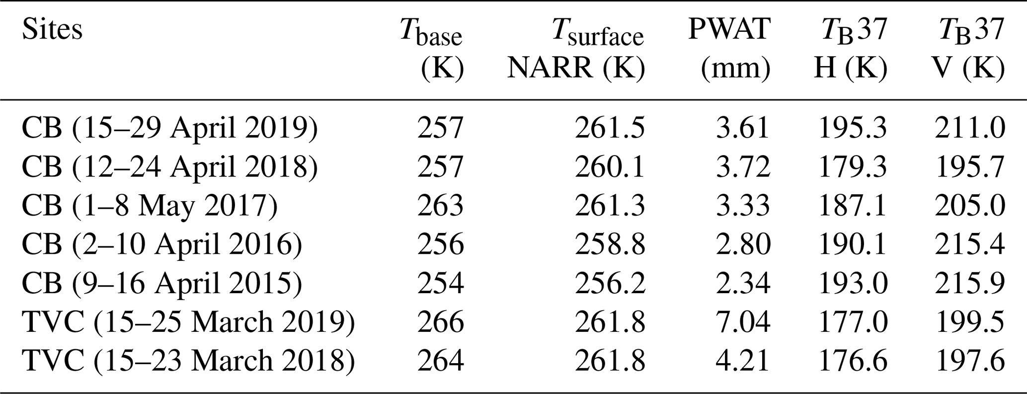
The basal layer temperature was set to the mean soil–DH interface measurements from snow pits of each site. The temperature of the WS layer was estimated from the North American Regional Reanalysis (NARR) air surface temperature, which closely matched snow pit surface layer temperature. NARR air surface temperatures were used because they provide a global estimate that matches spatial coverage of the EASE-Grid 2.0, which is continuous (spatially and temporally) compared to the sparse snow pit observations.

Table 2 Summary of mean basal and air surface temperatures for SMRT simulations, precipitable water (PWAT) used for atmospheric correction, and measured (corrected) T_B at both vertical (V) and horizontal (H) polarization by the SSMIS sensor (platform F18).

2.4 Gaussian processes

Gaussian processes (GP) are a non-parametric Bayesian method used in regression models. These processes are effective and flexible tools to fit complex functions with small training datasets (Quiñonero-Candela and Rasmussen, 2005). Gaussian processes provide uncertainties on predictions, using training data and prior distributions to produce posterior distributions for predictions. Mean (m(x)) and covariance (k(xx^′)) functions from the multi-variate Gaussian distribution are used to fit data (x: snow depth, y: ratio of layer, DHF). The m(x) function describes the expected value of the distribution, and the k(xx^′) describes the shape of the correlation between data points (x_i). Different mean and covariance kernels can be chosen to fit the data. From the Bayes rule in Eq. (1), where y (DHF) and X (snow depth) are observed data and f the GP function, posterior predictions of DHF can be produced. Posterior predictions were calculated using the standard method of Markov chain Monte Carlo (MCMC) sampling using PyMC3 (Salvatier et al., 2016).

$$\begin{array}{}\text{(1)}& {\displaystyle }\begin{array}{rl}\mathrm{Posterior}& ={\displaystyle \frac{\mathrm{likelihood}\cdot \mathrm{prior}}{\mathrm{marginal}\mathrm{likelihood}}}\\ & =p\left(f\mathrm{|}y,X\right)={\displaystyle \frac{p\left(y\mathrm{|}X,f\right)\cdot p\left(f\right)}{p\left(y\mathrm{|}X\right)}},\end{array}\text{(2)}& {\displaystyle }f\left(x\right)\sim \mathrm{GP}\left(m\left(x\right),k\left(x,x^{\prime }\right),\mathit{\varphi }(x\right)).\end{array}$$

Equation (2) defined f as a function of $m\left(x\right),k\left(x,x^{\prime }\right)$. A mean function m(x), following an inverse logic function (ϕ) (Eq. 3), was chosen due to the close fit with observations. The covariance function $k\left(x,x^{\prime }\right)$ is a Gaussian white noise covariance function and is defined with noise (σ) and the Kronecker delta function (δ_x,x) (Eq. 4), to best fit the observations. By using a scaling function (ϕ), the covariance function (uniform noise in this case) can be modified as a function of x. The scaling function used is also an inverse logic function (ϕ) that takes the same form as Eq. (3). Finally, a deterministic transformation is applied to the prior (GP) to constrain values to a ratio (0, 1). The likelihood of DHF observations is defined by a Beta distribution (0, 1).

$$\begin{array}{}\text{(3)}& {\displaystyle }m\left(x\right)=\mathit{\varphi }\left(x\right)=c+b\left[{\displaystyle \frac{e^{a\left(x-x_{\mathrm{0}}\right)}}{\mathrm{1}+e^{a\left(x-x_{\mathrm{0}}\right)}}}\right]\text{(4)}& {\displaystyle }k\left(x{x}^{\prime }\right)={\mathit{\sigma }}^{\mathrm{2}}{\mathit{\delta }}_{x,x^{\prime }}\mathit{\varphi }\left(x\right)\end{array}$$

3 Results

3.1 Snow depth distribution

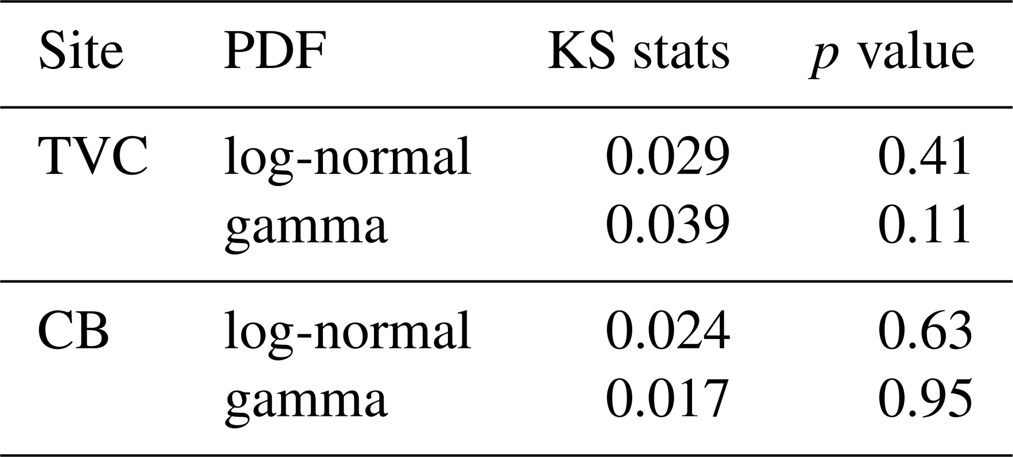
Distributions of snow depth are needed when integrating over large areas to calculate sub-grid snow variability for distributed models (Clark et al., 2011; Liston, 2004). The μ_sd and the CV_sd of snow depth are used as parameters in probability density functions to estimate the shape of the log-normal and gamma distributions. To find which distribution best fits the depth observations, we tested the log-normal and gamma distributions using the Kolmogorov–Smirnov two-sample test with snow depth observations (shown in blue in Fig. 2). The statistical fits for each distribution are shown in Table 3. For both the log-normal and gamma distributions the null hypothesis is validated at the 5 % significance level from p value > 0.05 (i.e., the two samples were drawn from the same distribution), which agrees with previous assessments of Arctic snow (Clark et al., 2011; Gisnås et al., 2016).

Table 3 Kolmogorov–Smirnov (KS) test for two samples of probability distribution function (PDF).

Figure 2 Log-normal and gamma distribution fit to the measured snow depths.

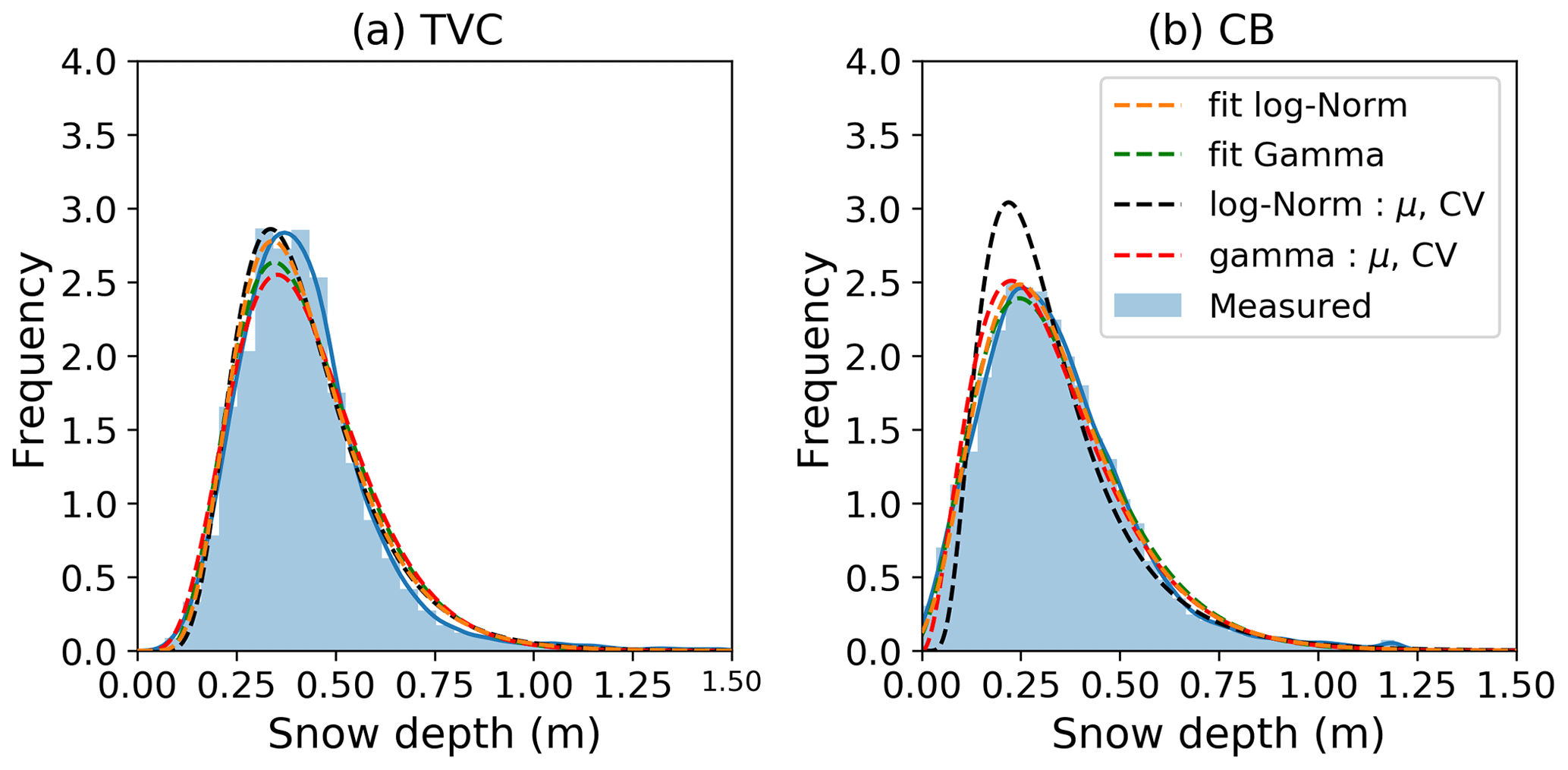
Distributions with parameterization using measured μ_sd and CV_sd (Fig. 2) differ from the best fit with regular parameters, especially compared with the log-normal distribution in CB (black dashed line in Fig. 2b). Liston (2004) reported a CV_sd of 0.4 for Arctic tundra snow, which is in close agreement with the values of 0.43 for TVC and 0.56 for CB. These values were obtained from spatially distributed snow depth measurements around snow pits. For comparison, maps of snow depth from RPAS for TVC (n= 6 325 365 with total spatial coverage of 5.3 km²) showed a much larger CV_sd= 0.78 than magnaprobe data (n= 15 731) with CV_sd= 0.43 (Table 4). A RPAS dataset was also available for CB but with a much smaller spatial coverage (0.2 km²) showing a CV_sd of 0.49. In Figs. 3 and 4, we investigated the relationship between spatial coverage of sampling and the CV_sd parameter. Datasets include RPAS-derived data at TVC (TVC18-RPAS) containing six areas with various size from 1–3 km², a CB18-RPAS map of 0.2 km² and the larger lidar-derived snow map in TVC (TVC13-Lidar). Figure 3a shows snow accumulation of TVC13-Lidar and TVC18-RPAS with snow drift visible in dark blue, and a sub-grid of 1 km² showed areas with high CV_sd (Fig. 3b) containing more drift. For both areas, 500 Monte Carlo simulations were performed by randomly selecting subregions within each domain (Fig. 4) so the mean and variability as a function of coverage could be investigated. Simulations showed subsampling of μ_sd and CV_sd converged to the values of the full area. The mean of each area was similar in value with less variation in the simulations compared to CV_sd. A difference of 0.2 between the full CV_sd of the RPAS (5 km²) and lidar (93 km²) maps (Fig. 4) was found. Also included in Fig. 4 are in situ CV_sd estimates with variable high-density sampling (magnaprobe) over different spatial extents at Daring Lake, NWT (Derksen et al., 2009; Rees et al., 2014); Puvirnituq, QC (Derksen et al., 2010); and at Eureka, NU (Saberi et al., 2017). The two points at the limit coverage scale correspond to areas of respectively 625 km² (CV_sd= 1, Daring Lake site; Chris Derksen, personal communication, 2009) and 198 km² (CV_sd= 0.89, Eureka site; Saberi et al., 2007).

Table 4 Statistical parameters of snow depth distributions. Bold font represents multi-year average.

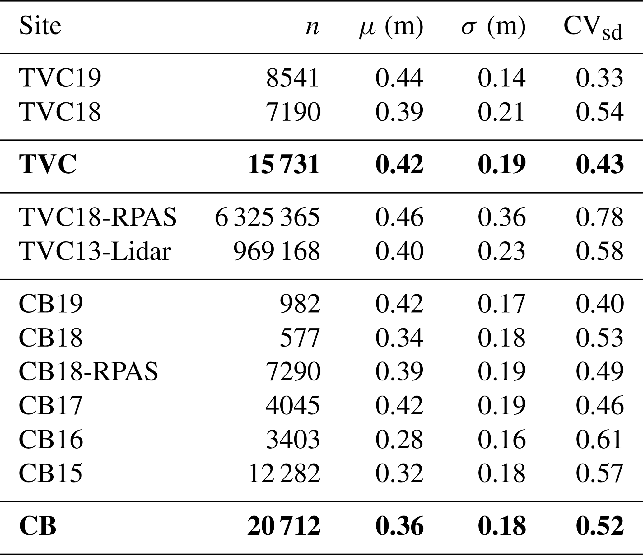
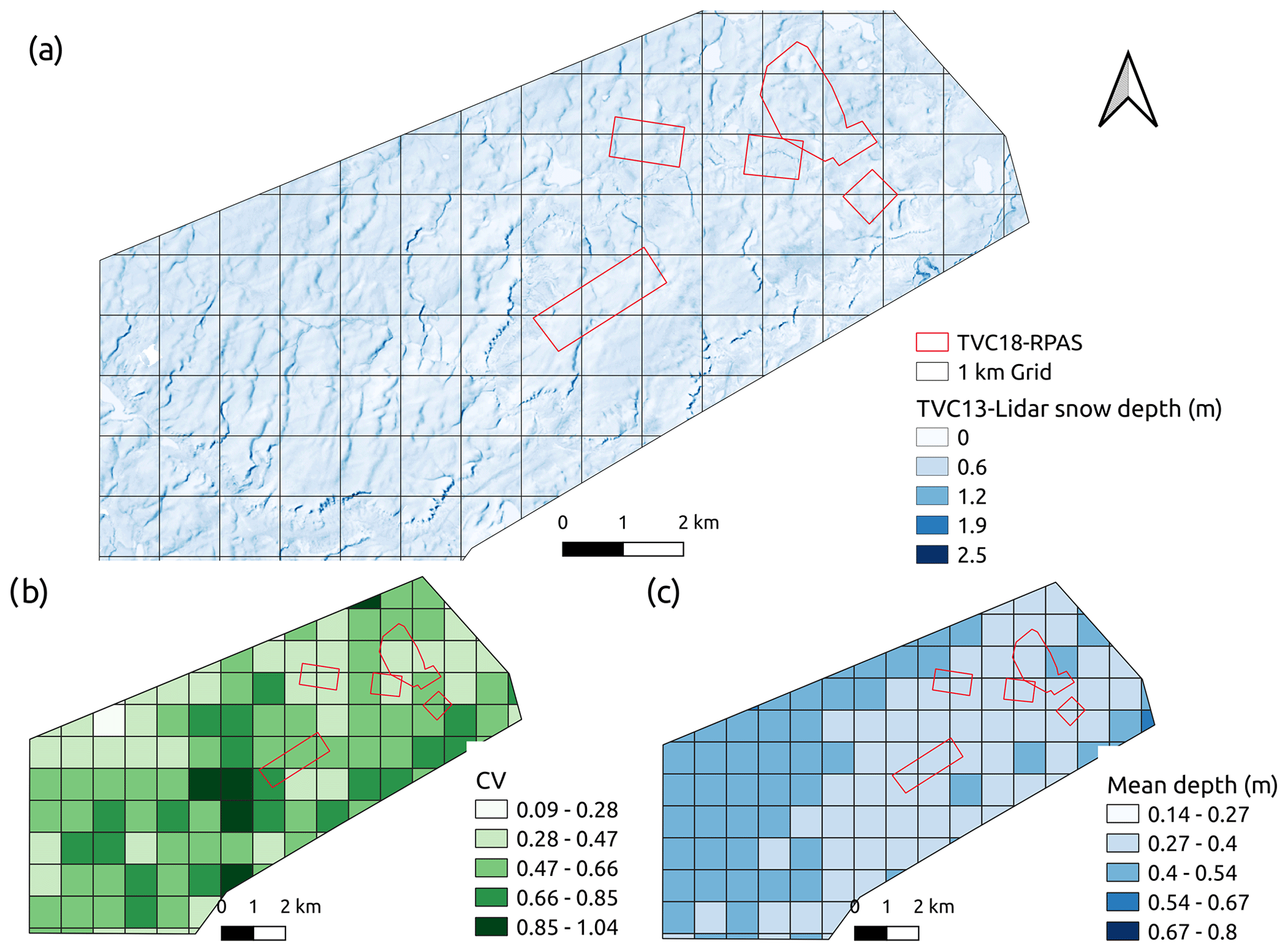
Figure 3 RPAS and lidar dataset of snow depth at TVC (TVC13-Lidar and TVC18-RPAS). TVC13-Lidar is the largest dataset covering 93 km². TVC18-RPAS is a smaller dataset within the area of TVC13-Lidar. Panel (a) shows the snow depth map at 10 m resolution from 2013. Panel (b) shows a sub-grid of 1 km with CV_sd for each cell; (c) same as panel (b) but for μ_sd.

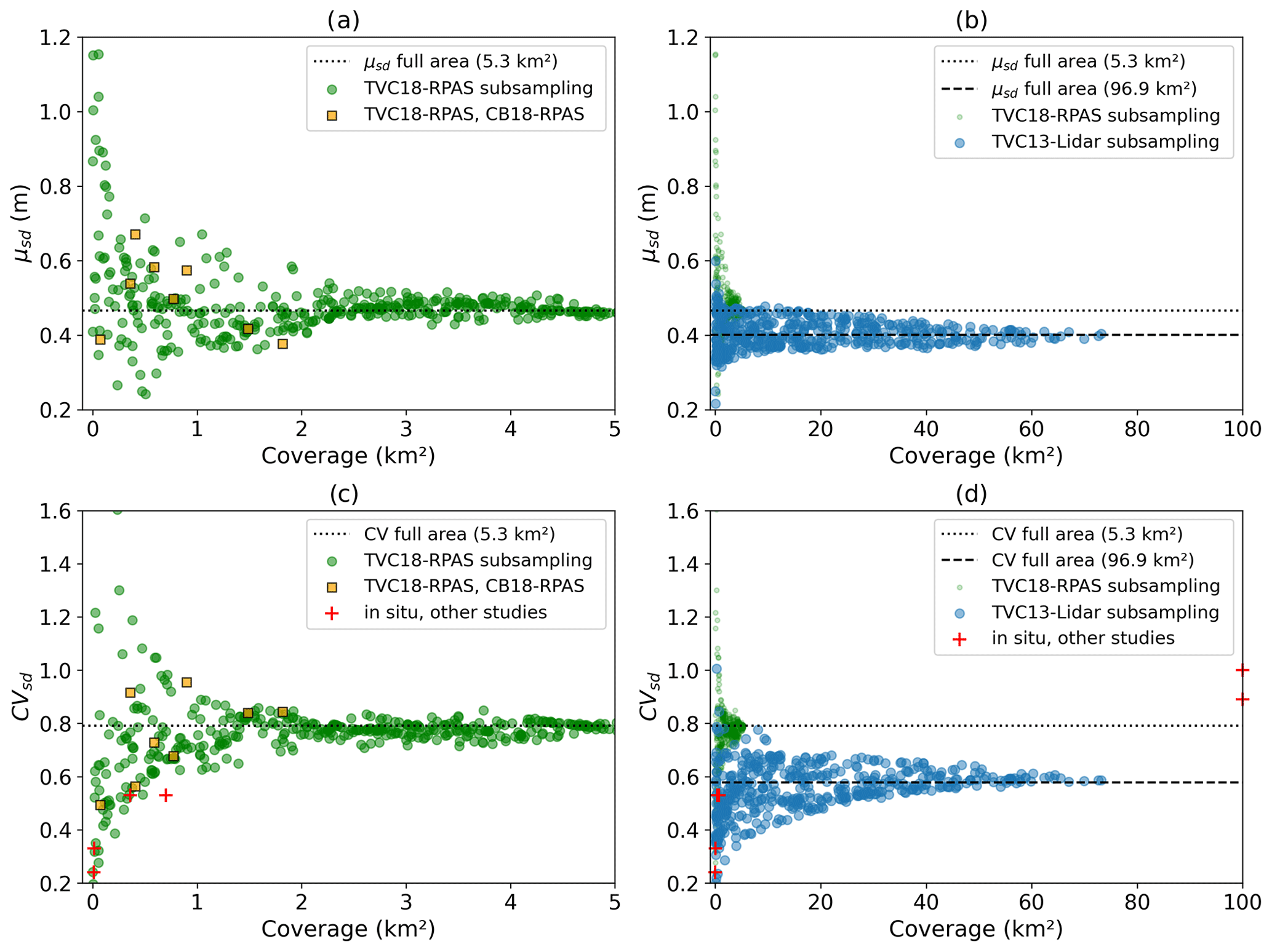
Figure 4 Snow depth mean (μ_sd) (a, b) and variability (CV_sd) (c, d) as a function of coverage for sampling area: (a, c) small area; (b, d) large area. Monte Carlo simulations were done using the two datasets in TVC. CB18-RPAS was also added in panels (a) and (c) because of the similar coverage. The μ_sd and CV_sd of both full areas are shown by the black dotted and dashed line.

3.2 Analysis of SSA and density per layer

After combining measurements from all snow pits at TVC and CB (n= 315) the mean proportion of DH layer thickness was 46 % and WS was 54 %. The goal was to classify DH as large grain snow (large facets, depth hoar cups and chains) and then all other snow layers above the DH as wind slab (WS). Some layers were more difficult to classify as they contained mixed crystals or were a transitional slab-to-hoar layer (also referred to as indurated hoar) (Derksen et al., 2009). Slab that contained small faceted crystals (< 2 mm) were classified as WS. Indurated hoar, a wind slab metamorphosed into depth hoar, was classified into DH with a typical density ∼300 kg m⁻³. For this reason, the peak of each distribution appeared close to each other in Fig. 5c and d. For retrieval of snow properties using satellite remote sensing, a two-layer model using WS and DH can be used to simplify much of the layer complexity found in arctic snowpacks (Rutter et al., 2019; Saberi et al., 2017). A small amount of surface fresh snow (SS) was present in some pits but was not included in this calculation as this type of snow was a short-lived layer, combining fresh precipitation that rapidly transformed into rounded grains due to destructive metamorphism and defragmentation by wind. Distributions of SSA are more distinct between layers than density (Fig. 5a and b); see Rutter et al. (2019). Figure 5c and d show that the mean values for density of WS (335 kg m⁻³) and DH (266 kg m⁻³) were closer together. SSA distributions also showed a gap between both mean values (WS: 19.7 m² kg⁻¹; DH: 11.1 m² kg⁻¹) (Fig. 5, Table 5). Even if snow properties can show high heterogeneity at local scales, simple distributions approximate this variability well. Temporal (year) and spatial (regional between site) variation is low, and snow properties (density and SSA) can be approximated by a distribution for each distinct layer, WS and DH as in Fig. 5. Therefore, snow properties were simplified in distributions for each layer (WS and DH) representing tundra snow.

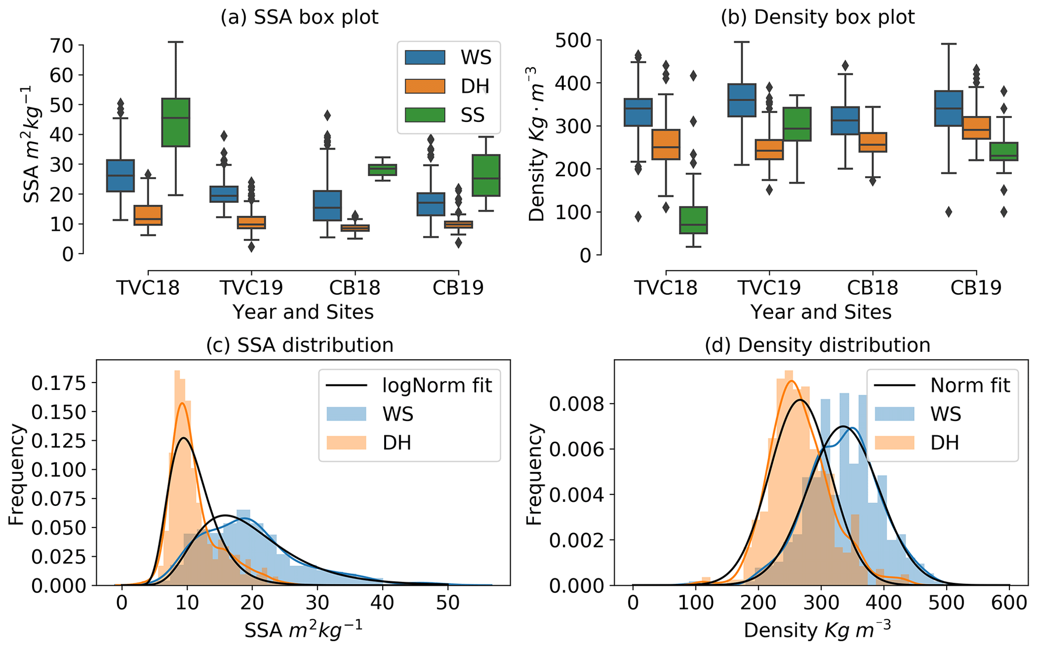
Figure 5 SSA and density variability of surface snow (SS), wind slab (WS) and depth hoar (DH) for the two studied sites (TVC and CB) and different dates (see Table 5). In panel (c) the best log-normal fit distribution is shown in black; (d) same as panel (c) but for the normal fit distribution. In panels (c) and (d), the kernel density estimates (KDEs) of the histogram of each layer are also shown (in color).

Table 5 Parameters for best fitting distribution of SSA and density for layers of DH and WS.

Parr et al. (2020) found a key threshold of μ_sd+1σ_sd to define snow drifts in tundra environments. This threshold (> 0.6–0.8 m), based on data presented in Table 4, is an important metric in Fig. 6 since above this depth the variability and the mean DHF are greatly reduced as the snowpack is dominated by wind slab for larger depth (drift). As defined in Parr et al. (2020), the transported snow from wind accumulates at these particular locations (drift) where it was scoured from wind affected area yielding lower depth with high DHF.

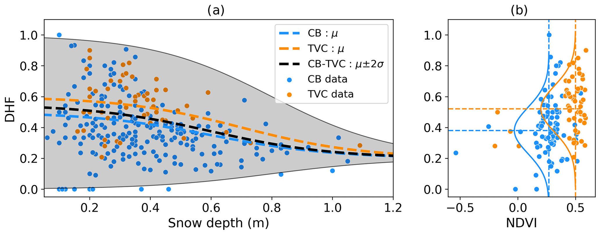
Figure 6 (a) Depth hoar fraction (DHF) as a function of total depth for snow pit data from 2015–2019 in Cambridge Bay and 2018–2019 for Trail Valley Creek. Both datasets were separated in equal bins (10 cm) to estimate the mean value shown with the dashed line. The black line represents the mean for both sites with the 95 % confidence interval. (b) DHF is shown as a function of NDVI from the snow pit area with the mean DHF and NDVI per site shown by dashed lines and the Gaussian distributions of DHF by the solid lines.

Vegetation also strongly influences variability of DHF in shallower snowpacks, where arctic shrubs and tussocks promote depth hoar formation (Domine et al., 2016; Royer et al., 2021; Sturm et al., 2001). However, there is no clear link between DHF and NDVI (a proxy for vegetation type) at local scales (Fig. 6b). Since shrubs provide shelter to snow up to their own height (Gouttevin et al., 2018), vegetation height rather than type would be required. However, at the regional scale, differences were evident between both regions, where mean NDVI and DHF are greater at TVC (NDVI = 0.5, DHF = 0.54) than CB (NDVI = 0.27, DHF = 0.38). This finding is in agreement with Royer et al. (2021) over a northeastern latitudinal gradient, showing that sites with shrubs and tussocks have a greater DHF than those without.

3.3 DHF predictions using snow depth with Gaussian processes

The impact on microwave scattering of variability of layer microstructures with snow depth was previously accounted for in Saberi et al. (2020) by defining two categories, a high scattering thin snow layer (high DHF) and a thicker self-emitting layer (low DHF). Instead, using GP, DHFs were fitted and predicted based on snow depth values (Fig. 7). In order to use GP, the mean function m(x), following an inverse logic function (ϕ₁: Eq. 3), was chosen with parameters $a=-\mathrm{5}$, x₀=0.6, b=0.35 and c=0.2 to best match the mean line observation for both sites in Fig. 6. The mean function set the mean value across the snow depth range. The correlation function was set to a uniform noise, but this noise was reduced from depth > 40 cm by using a scaling function (${\mathit{\varphi }}_{\mathrm{2}}:a=-\mathrm{5}$, x₀=0.6, b=1.5 and c= 0.25). An inverse logic function (ϕ₁, ϕ₂) was used twice in the fitting (1) for the mean value and (2) to reduce the variability (noise) as snow depth increased. The snow pit dataset (n= 315, Fig. 6) was used to build posterior predictions using MCMC sampling.

For prediction of DHF, any number of snow depths can feed into the posterior prediction or GP fit. Snow depths were generated from a log-normal distribution with parameters (μ_sd, CV_sd) from the previous section in Table 4. Posterior predictions of DHF were similar to observed data (Fig. 7) and followed closely the posterior probability representation in red (GP fit). Again, higher variability in DHF was reproduced for depths < 0.5 m, which was then reduced for depths > 0.5 m following the red posterior prediction representation in Fig. 7.

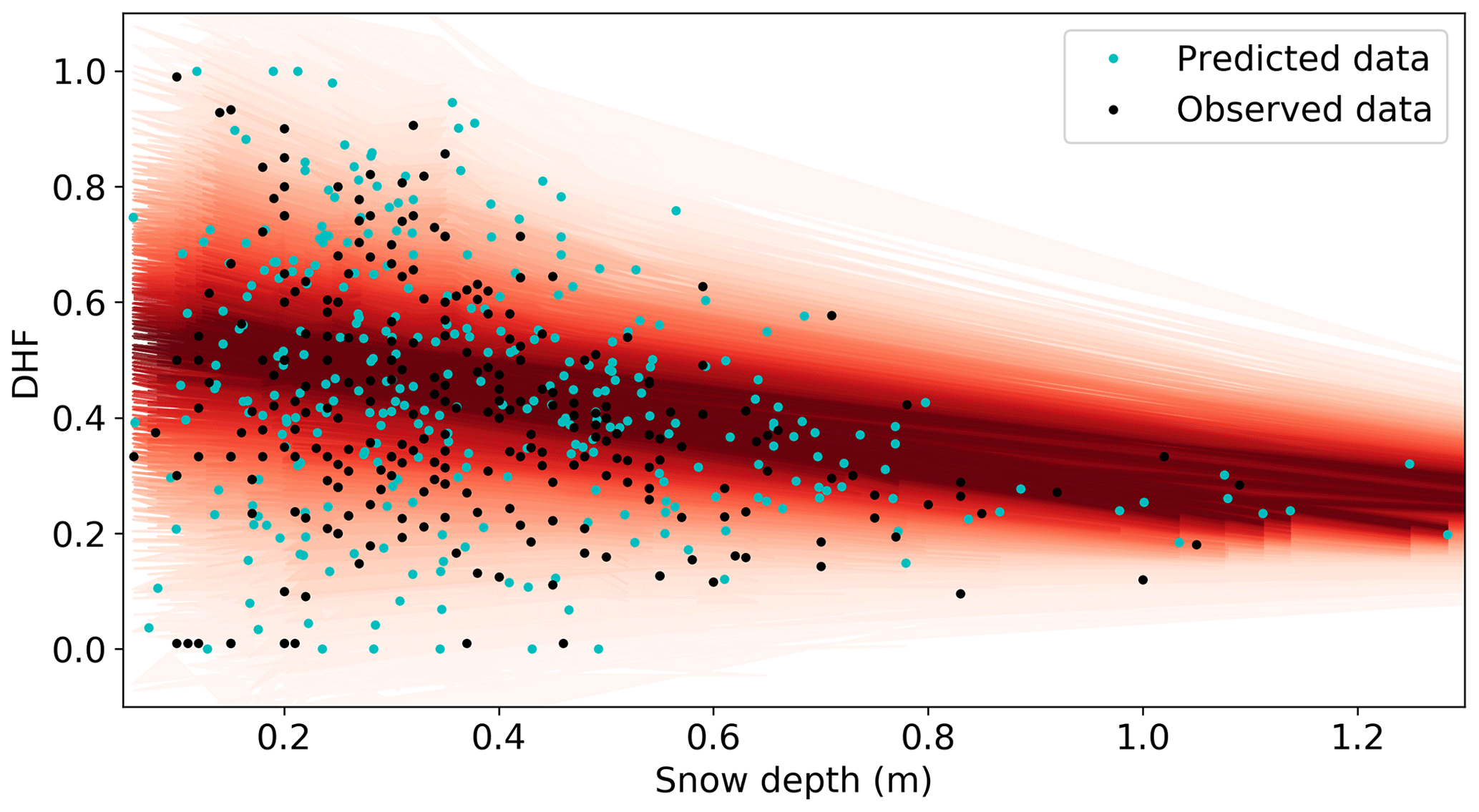
Figure 7 Prediction on DHF (cyan) using a GP fit trained on observed data (black). Snow depth is from samples from a log-normal distribution with parameters from Table 4. The GP fit is illustrated in red, where darker red represents a high posterior probability that follows the mean function.

3.4 SMRT simulation of sub-grid variability within sensor footprint

SMRT simulations using measured snowpack properties were compared with the satellite measurements of T_B. Two simulations were evaluated using (1) mean measured depth, each layer's density and SSA, and DHF and (2) a log-normal distribution of snow depth and the GP fit (predicted DHF). We hypothesized that the EASE 2.0 grid pixels can be separated into n smaller sub-grid pixels. Sub-grid pixels (n= 500) represent the observed snow variability, where n snow depths will follow a log-normal distribution with parameters μ_sd and CV_sd. The ratio of each layer is predicted using the GP fit with depth as input from the log-normal distribution. Mean SSA (DH: 11 m² kg⁻¹; WS: 20 m² kg⁻¹) and density (DH: 266 kg m⁻³; WS: 335 kg m⁻³) per layer were determined from measurements (Fig. 5).

For one standard EASE-Grid 2.0 pixel, a distribution of sub-grid T_B was simulated to reproduce a realistic distribution of T_B within the radiometer footprint. This variability was derived from spatially distributed observations from snow pits and snow depths observation. Snow depths followed a log-normal distribution with the mean measured depth (μ_sd) of each region (Table 4) and a depth variability (CV_sd) that was evaluated from a range of 0.1 to 1. The GP mean function from Fig. 7 was used to predict the DHF for each region. When using CV_sd= 0.7 , the simulated distribution showed a wide sub-pixel variability (±40 K) with a mean value of T_B37V= 194.7 K (blue line in Fig. 8a), which is very close to the satellite-measured T_B37V of 196.5 K (green dotted line in Fig. 8a). In this case, the T_B value simulated from the mean measured snow depth and mean DHF was slightly lower (190.7 K, i.e., a bias of 5.8 K) (black dotted line in Fig. 8a). To represent the signal measured by the sensor, the mean of the simulated T_B was chosen, and it was assumed that the sub-pixel effect combined linearly at this scale. Because the simulated T_B37V distribution was not exactly a normal distribution, it appeared that the mean T_B of this distribution increased when CV_sd increased (Fig. 8b). This meant that snow depth variability (CV_sd) must be accounted for when estimating the average T_B at 37 GHz, in addition to the mean snow depth values. The influence of the GP simulation on the mean simulated T_B37V was approximately 10 K (Fig. 8b) as CV_sd varies from 0.1 to 1. The addition of snow variability in simulation (Fig. 8c and d) of 19 GHz has negligible effect on T_B19 and shows a constant simulation across the CV_sd range of 0.1 to 1. Simulation of T_B19 shows higher biases at horizontal polarization than at vertical polarization.

Figure 8 Brightness temperature variability simulation distribution (a, c) of simulated T_B within a pixel, where vertical lines represent the mean of this distribution for V pol (blue), measured by satellite (green), and T_B value simulated from the mean measured snow depth and mean DHF (black). In panels (b) and (d), the mean of the simulated T_B for H pol (red) and V pol (blue) as a function of CV_sd with mean values (dotted black lines). The CV_sd that minimized biases is located at the red/blue–green intersection. Shaded blue and red areas correspond to a 2σ range representing uncertainty inherent from our Bayesian simulations in estimating the mean of simulated T_B for the pixel.

GP simulation reduced biases by 5 K with a higher optimized CV_sd (intersection of red/blue–green line, Fig. 8b). A similar pattern was observed for CB (not shown here), but the measured T_B at CB was much higher than the GP simulation, resulting in a large bias for CB (∼ 20 K) compared to TVC (Table 6). Both sites suggested a larger CV_sd, which agreed with a CV_sd for larger spatial coverage measured in Fig. 4. Observed large biases at CB vary over the years from 5 to 29 K. The total RMSE of both sites and years linearly decreased as a function of CV_sd (Fig. 9). Total RMSE is minimized with higher CV_sd (0.8–0.9) typical of a large sampling scale (over 4 km²) as shown in Fig. 4.

Table 6 Bias between SMRT simulated and measured T_B from the SSMIS sensor at each site.

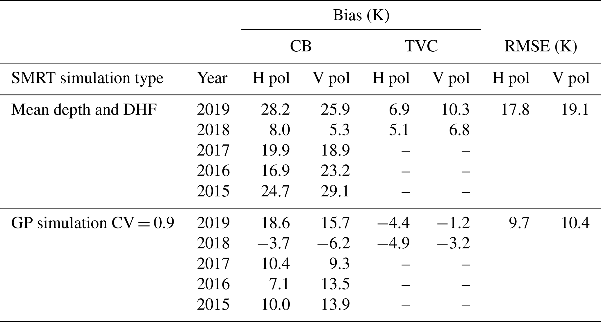
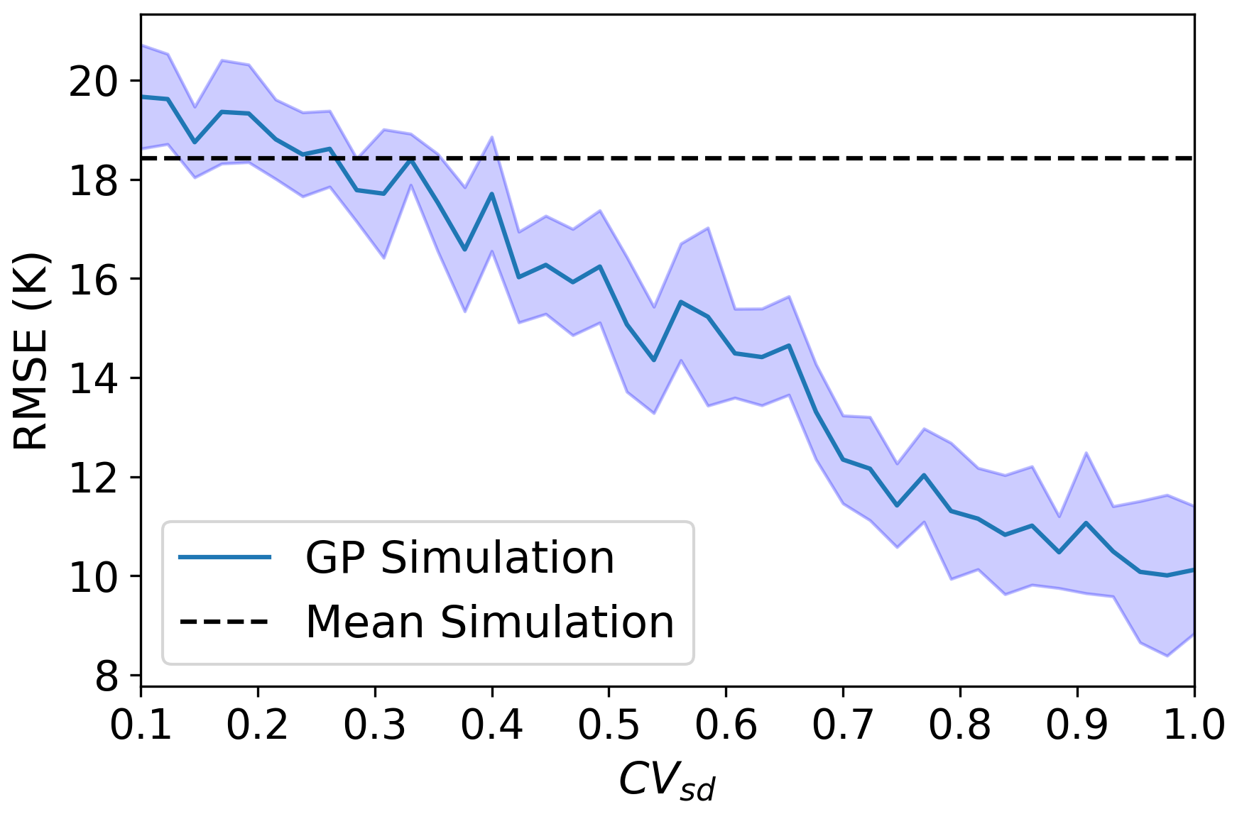
Figure 9 Overall RMSE (year and site) with the mean simulation (dashed black line) and the GP simulation in blue as a function of the coefficient of variation of snow depth.

4 Discussion

We show that as spatial coverage increased, the CV_sd parameter converged to the full area values (Fig. 4). Monte Carlo simulations of snow depth distribution and coverage show high variation in CV_sd (from 0.1 to 2) for areas < 10 km². Snow accumulation varied at the mesoscale (100 m to 10 km) due to topography and vegetation (Pomeroy et al., 2002) by varying wind-flow direction (Liston and Sturm, 1998). At the mesoscale, variability in CV_sd was high due to topographic differences; plateau, slope and valley create favorable conditions from wind-flow direction to promote snowdrift, scour and sublimation processes (Parr et al., 2020; Rutter et al., 2019). Vegetation facilitates snow holding capacities by decreasing wind speed near the ground within and downwind of shrub (Marsh et al., 2010; Sturm et al., 2001). Some areas include both extreme drifts and thin snow, resulting in high CV_sd (dark green areas in Fig. 3b), which are commonly found in TVC (Walker et al., 2020a). CV_sd was lower for areas without drifts (light green areas in Fig. 3b). In areas >10 km² (Fig. 4d), variation in CV_sd was reduced and yielded higher values > 0.6.

Convergence to higher CV_sd as spatial coverage increased matched the PMW optimized values found in this study using GP simulation (0.8–1.0). Our analysis in Fig. 4d showed that CV_sd of TVC13-Lidar converged to 0.6 at 93 km², but two in situ points from other studies at 625 km² had higher CV_sd (0.9–1) due to larger coverage or different site characteristics. This indicates that a CV_sd between 0.6–1.0 is more suitable to represent snow depth variability in SWE retrievals for PMW SWE products at 25 km for the EASE-Grid 2.0 and 625 km² for GlobSnow 3.0 (Pulliainen et al., 2020). For active sensors (resolution < 1 km), the high variability in CV_sd under 1 km² due to high variation in snow depth (Fig. 4b) can affect back scattering since the active sensor at the Ku band is also sensitive to volume scattering (King et al., 2018). The need for prediction of μ_sd and CV_sd based on topography could become essential at these scales not only for microwave remote sensing but also to improve snow modeling or land data assimilation (Kim et al., 2021).

Spatial complexities of Arctic snowpacks can be adequately characterized with distributions of snow depth (Fig. 2) and simplified by considering density and SSA of two main layers (Fig. 5). Such simplifications could be potentially useful for satellite SWE retrievals across Arctic tundra regions. Since Bayesian SWE optimization needs a strong first guess from regional a priori information, multiple distributions of snow depth, density and SSA presented here can be used for tundra type snow in MCMC sampling (Pan et al., 2017; Saberi et al., 2020). Additionally, a similar approach to our GP simulation can be added so the CV_sd parameter can also be used as a priori information with a distribution from 0.8 to 1, since it improved T_B RMSE by ∼8 K (Fig. 9). This approach improved T_B simulation compared to using only mean values of snowpack properties by adding variability within the footprint. The CV_sd parameter (describing variation in snow depth) has a considerable effect on brightness temperature (10 K) when used as an effective parameter to account for sub-pixel variability of snow depth. The amount of scatterers (snow grain and structure) within the radiometer's footprint is adjusted via the DHF predicted from snow depth (CV_sd). The relationship found in Fig. 6 used to predict DHF (Fig. 7) could also be used deterministically with the mean function (ϕ₁) or with a linear relation of DHF decreasing from 50 % to 20 %. However, the Bayesian Gaussian process was used because SWE retrievals are currently implemented in a Bayesian framework (Takala et al., 2011).

Considering that the difference between 19 and 37 GHz is used in SWE retrievals (Takala et al., 2011), using the CV_sd to account for variability of scatterers only affected simulation of 37 GHz with a weak effect on 19 GHz (Fig. 8). If standard deviation of snow increases (more drift), then relatively fewer large scatterers from depth hoar are present within the footprint due to a low DHF generally observed in large drifts. The net result is then an increase in T_B at 37 GHz resulting from an increase in CV_sd (Fig. 8).

This idea of modulating the amount of scatterers based of DHF prediction and a distribution of snow depth (μ_sd and CV_sd) can be extended to a future active Ku-band mission (Garnaud et al., 2019; King et al., 2018) as it is known that microwave spatial variability affects backscatter signal (King et al., 2015) and SWE retrievals (Vander Jagt et al., 2013). The CV_sd parameter is proposed as an effective parameter to account for variability inside the grid cell, while the mean depth (μ_sd) is assimilated by in situ measurements at weather stations in data assimilation schemes (Takala et al., 2011) or by the physical snow model (Larue et al., 2018). The CV_sd could be optimized or predicted using relationships with spatial coverage (Fig. 4) and statistical topographic regression (Grünewald et al., 2013). Future works would need a dataset covering a large area where μ_sd and CV_sd could be investigated with topography in smaller sub-areas.

5 Conclusion

This study evaluated the use of parameters controlling Arctic snow depth distributions to improve passive microwave SWE retrievals by characterizing tundra snow sub-pixel variability. In shrub and graminoid tundra environments, mean values of snow depths (μ_sd= 0.33–0.44 m) and coefficient of variations (CV_sd= 0.4–0.8) were similar to those previously reported in Arctic tundra (Derksen et al., 2014; Liston, 2004; Derksen et al., 2009). Monte Carlo simulations were applied to investigate μ_sd and CV_sd as a function of spatial coverage. An increase in CV_sd matched increased spatial coverage of snow depth sampling, indicating that a higher CV_sd (0.6–0.9) is more suited to estimate snow depth variation at the 3.125 km resolution EASE-Grid 2.0. Also, simulations show high variation in CV_sd (> 0.9) for areas < 10 km², suggesting a need for topography-based prediction of μ_sd and CV_sd at this scale. The CV_sd is shown to be an effective parameter to account for snow depth variability in simulation of snow T_B. A two-layer snowpack model (depth hoar and surface wind slab), which simplifies snowpack properties into distributions, was used to initialize the SMRT model via a GP fit of the DHF related to snow depth. DHF is fitted to snow depth using a Bayesian Gaussian process, which accounts for variation in snow scattering using CV_sd. SMRT simulation was used successfully to simulate satellite T_B, but there are still substantial uncertainties in the simulated values which are likely linked to microstructural properties not captured by SSA (Krol and Löwe, 2016). SMRT simulations of T_B were reduced by 8 K after optimizing CV_sd to higher values (0.8–1.0), thereby matching CV_sd of spatially distributed snow depth from TVC18-RPAS accounting for variation in snow properties inside the footprint of satellite sensor. The CV_sd parameter is proposed as an effective parameter to account for variability inside the footprint to minimize the difference between microwave measurements and simulations in SWE retrievals algorithm. This would be beneficial to the data assimilation scheme of the European Space Agency GlobSnow product (Takala et al., 2011) and to model the large-scale climate trend of tundra snow (Mortimer et al., 2020; Pulliainen et al., 2020).