the Creative Commons Attribution 4.0 License.
the Creative Commons Attribution 4.0 License.
 | 11 Mar 2022
The importance of freeze–thaw cycles for lateral tracer transport in ice-wedge polygons
Elchin E. Jafarov
Daniil Svyatsky
Brent Newman
Dylan Harp
David Moulton
Cathy Wilson
A significant portion of the Arctic coastal plain is classified as polygonal tundra and plays a vital role in soil carbon cycling. Recent research suggests that lateral transport of dissolved carbon could exceed vertical carbon releases to the atmosphere. However, the details of lateral subsurface flow in polygonal tundra have not been well studied. We incorporated a subsurface transport process into an existing state-of-the-art hydrothermal model. The model captures the physical effects of freeze–thaw cycles on lateral flow in polygonal tundra. The new modeling capability enables non-reactive tracer movement within subsurface. We utilized this new capability to investigate the impact of freeze–thaw cycles on lateral flow in the polygonal tundra. Our study indicates the important role of freeze–thaw cycles and the freeze-up effect in lateral tracer transport, suggesting that dissolved species could be transported from the middle of the polygon to the sides within a couple of thaw seasons. Introducing lateral carbon transport into the climate models could substantially reduce the uncertainty associated with the impact of thawing permafrost.
- Article
(2629 KB) - Full-text XML
- BibTeX
- EndNote


Permafrost stores a vast amount of frozen carbon, which, once thawed, can be released into the atmosphere, amplifying current rates of global warming (McGuire et al., 2018). More than a quarter of the total carbon found in permafrost is stored in tundra ecosystems characterized by organic carbon-rich soil (Strauss et al., 2013). Understanding the impact of permafrost hydrology on the subsurface transport of dissolved carbon is crucial for reducing the uncertainty associated with quantifying the permafrost carbon feedback (Hinzman et al., 2000; Liljedahl et al., 2016; Andresen et al., 2020). A recent study by Plaza et al. (2019) indicates that lateral subsurface flow can be responsible for more than half of the permafrost carbon loss, but many models only consider vertical transport. Because lateral transport of carbon is significant, it is important to understand controls on the lateral transport so that the ultimate fate of transported carbon can be ascertained. Not only is the rate of carbon transport important for understanding fluxes to lakes and rivers, for example, but lateral transport conditions will also affect how carbon is cycled along a flow path and what form that carbon might ultimately take (e.g., carbon dioxide, methane, or dissolved organic carbon). A review by O'Donnell et al. (2021) highlights several studies that demonstrate a variety of Arctic flow and transport conditions that affect dissolved organic carbon (DOC) and nutrients such as nitrogen and phosphorous. For example, DOC fluxes typically increase during spring snowmelt where substantial lateral flushing occurs. After snowmelt, DOC fluxes tend to decrease, especially when active layers deepen into mineral soil layers. DOC compositions also shift as lateral flow through mineral soils increases or mixing with deeper groundwater sources becomes more important. Microbial utilization of DOC and nutrients can change concentrations along hydrological flow paths, and if redox conditions vary with depth or laterally, profound changes in concentrations and/or the geochemical forms of carbon (and nutrients) can result. Thus, incorporating lateral carbon fluxes into the existing climate models can significantly improve our current understanding and quantification of the permafrost carbon feedback.
In permafrost landscapes, the active layer is the top layer of soil that thaws during the summer. Modeling transport within the active layer remains a challenging problem because of the effects of liquid/ice phase change on transport. Dissolved constituents, including organic carbon, nutrients, redox-sensitive species (e.g., iron and methane), mineral weathering products, and contaminants, are all transported to varying degrees within the active layer during the thaw season and are immobilized when the soil freezes. Early research on transport within the active layer used a one-dimensional approach (Raisbeck and Mohtadi, 1974; Corapcioglu and Sorab, 1988). Hinzman et al. (2000) used the SUTRA numerical model to simulate benzene transport at Fort Wainwright, near Fairbanks, Alaska. That study showed that including permafrost in the simulation strongly influenced the tracer migration pathways. Recently, Frampton and Destouni (2015) applied a coupled subsurface heat and flow model to study the effect of thawing permafrost on tracer transport under different geological conditions.
Since there were previously no data showing tracer transport in the polygonal tundra, the Next-Generation Ecosystem Experiments (NGEE) Arctic team conducted a detailed tracer test on a low- and high-centered polygon at the Barrow Environmental Observatory (BEO) site at North Slope, Alaska. The team conducted a 2-year tracer experiment and collected the data on transport in polygonal tundra (Wales et al., 2020). Polygonal tundra is characterized by high- and low-centered polygon types but with corresponding microtopographic polygon features (troughs, rims, and centers). These surface expressions often follow changes in subsurface structure (i.e., ice wedges and frost table topography), affecting transport pathways. The results of this tracer experiment indicated complex tracer flow in both polygon types, suggesting heterogeneous soil conditions and a higher lateral rate of tracer flux in the low-centered polygon than in the high-centered polygon. Wales et al. (2020) suggested that freeze-up could promote additional tracer movement in the active layer of the low- and high-centered polygon. The freeze-up period is the time during which the active layer begins to refreeze until it freezes completely. The goal of this study is not a direct comparison with the existing data; instead, we test the hypothesis using a numerical model postulated as a result of tracer transport observations described in Wales et al. (2020).
We developed a new subsurface transport capability in an existing thermal hydrology permafrost model to investigate the effect of freeze–thaw dynamics on the lateral transport of a non-reactive tracer in the polygonal tundra. To test the impact of the freeze–thaw cycle on tracer transport, we set up two model configurations: freeze–thaw disabled and freeze–thaw enabled (Fig. 1). The freeze–thaw-disabled setup is a simplified version of a permafrost model, where a fixed impermeable layer represents permafrost and there is no ground freezing or thawing. In this setup, we run the model only during the thaw season (i.e., ground temperatures stay above 0 ∘C). The freeze–thaw-enabled setup includes a dynamically moving freeze–thaw boundary, and we run the model over a full-year cycle. We tested these two setups on two main types of polygonal tundra: high- and low-centered polygons. We complemented high- and low-centered polygon simulations with a flat-centered one to compare the effect of surface geometry on tracer mobility. This comparison emphasizes the effect of freeze–thaw dynamics on transport in permafrost soils. We further discussed the impact of subsurface properties on the tracer transport in the polygonal tundra, drawing parallels with the experimental study, and described the possible implications. It is important to note that this study focuses on non-reactive “tracer” transport because this is an essential basis for characterizing polygon hydrology. However, it does not represent reactive transport conditions that are critical for modeling solutes such as DOC or nutrients. In other words, the non-reactive transport models described here are a step toward more sophisticated models that include processes such as changing source contributions along a flow path, dissolution/precipitation, sorption phenomena, and microbial/redox processes.
2.1 The model
We developed a new subsurface non-reactive transport capability in the Advanced Terrestrial Simulator (ATS), a numerical simulator that simulates coupled hydrothermal processes in the permafrost environment (see Appendix). The ATS is a 3D-capable coupled surface/subsurface flow and heat transport model representing the soil physics needed to capture permafrost dynamics, including water flow in variably saturated, partially frozen, non-homogeneous soils (Painter et al., 2016). The ATS tracks water in its three phases (ice, liquid, and vapor) and simulates the transition between these phases in time. The introduction of tracer transport capability into the ATS enables numerical investigation of the processes influencing lateral non-reactive tracer transport in permafrost landscapes, including polygonal tundra, which was previously impossible.
2.2 Mathematical description of the transport equation in the ATS
The ATS transport model allows for tracer diffusion/dispersion capabilities. However, in this study, we focus on the effect of freeze–thaw on advective transport only. While the diffusion/dispersion processes would lead to additional spreading beyond the advective transport presented here, our results capture the general effect of freeze–thaw on transport in polygonal tundra. The partial differential equations describing advective surface/subsurface transport of the non-reactive tracer have the following form:
Here, ϕ is porosity [–], ρl is liquid molar density [mol m−3], sl is liquid saturation [–], δl is ponded water depth [m], γl is the effective unfrozen water fraction [–], Cl is the tracer molar fraction [–], is a source or sink term of the tracer in the subsurface domain [mol s−1 m−3] (we inject tracer into the top layer of the subsurface domain), and represents the mass of the tracer being exchanged from the surface to subsurface [mol s−1 m−2]. For the subsurface domain, the term is treated as a boundary condition, while for the surface domain this term is considered a source/sink term. Vl and Ul are subsurface and surface liquid velocities which are defined by Darcy's law and its surface analog, respectively, as follows:
Here, kl is a relative permeability which depends on the liquid pressure pl. K is the absolute permeability, and μl is the liquid viscosity. nman is Manning's roughness coefficient, and ∇Zs is the surface slope; ε is a regularization parameter.
It is common for multiphysics applications to use different time discretization schemes for different physical processes. Since thermal hydrology and transport have different timescale characteristics, it can be advantageous to use an explicit time discretization scheme for the transport processes. In contrast, the fully coupled thermal hydrology model is treated implicitly in time in the ATS. An explicit time approximation scheme requires much less computational time than an implicit one, but to be stable, additional time step restrictions should be imposed. The first-order upwind scheme is applied for the explicit discretization of the transport equations, Eqs. (1) and (2). The divergence operator is discretized using integration over the surface of a cell (Gauss theorem). In the first-order upwind scheme, a value of tracer mass is taken from the upwinding cell with respect to flow velocity to discretize the surface integral. For this discretization approach, the stable time steps for surface and subsurface domains should satisfy the following conditions:
where uout is the total outflux from a particular cell and |vcell| is the volume of the cell.
The selection of time step criteria depends on the surface flow speed and the amount of liquid saturation in a cell. These restrictions may lead to expensive and prohibitive computational costs, particularly for long-time integration problems. So, it is critical to be able to perform several transport time steps during one hydrology time step, and this procedure is referred to as subcycling. The interface term should be the same in Eqs. (1)–(2) to guarantee mass conservation during subcycling. Therefore, the same time step must be used in the surface and subsurface, although the time step restrictions can be different in these domains. The dataset that includes all the ATS input and visualization scripts used in this study is documented in Jafarov and Svyatsky (2021).
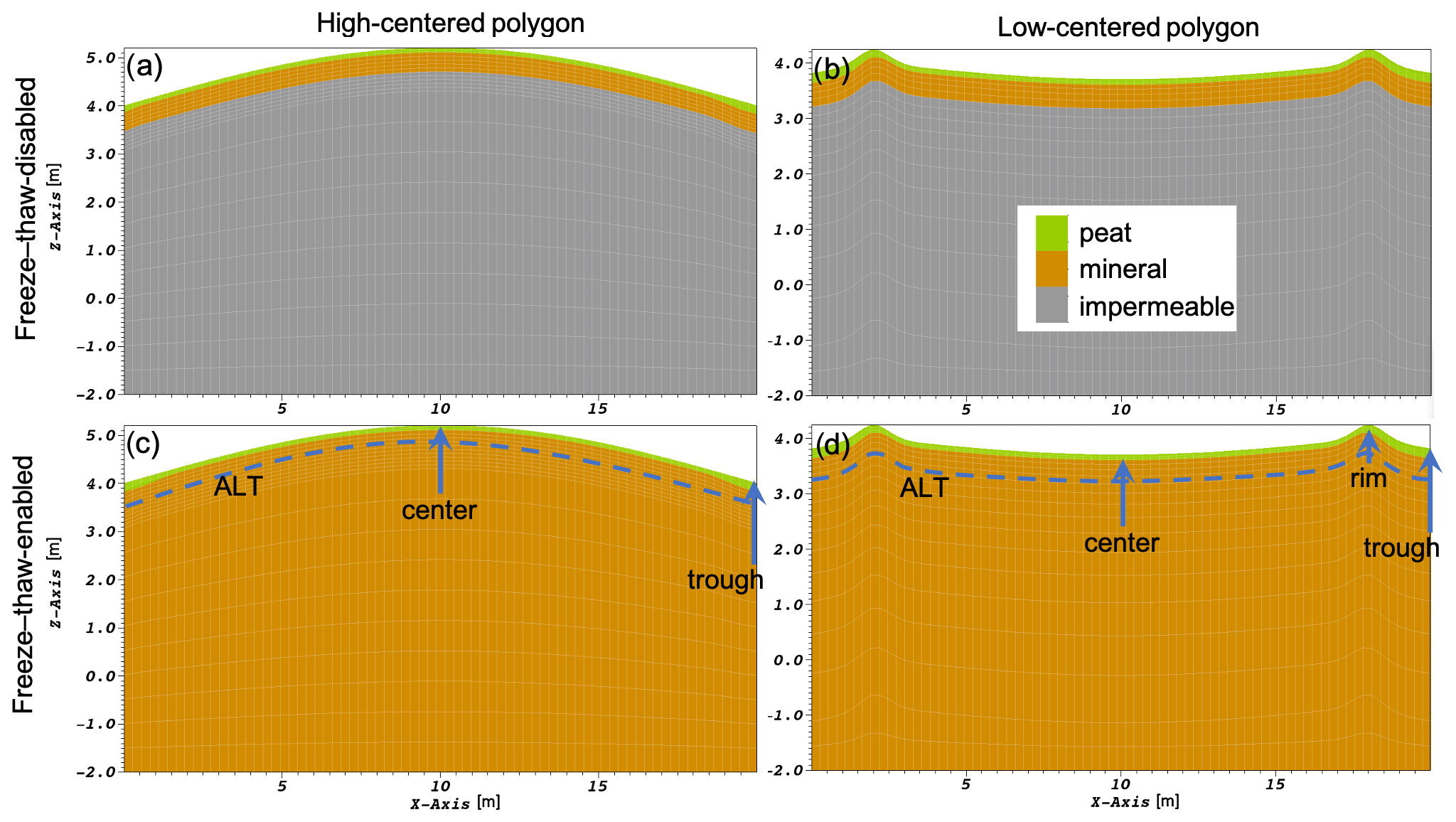
Figure 1ATS meshes of 2D transects of a high-centered polygon (a, c) and a low-centered polygon (b, d). The top row illustrates the stratigraphies representing the freeze–thaw-disabled case and the bottom row the freeze–thaw-enabled case. The green represents peat, brown the mineral soil layer, and grey the impermeable layer of the freeze–thaw-disabled case.
2.3 Setup
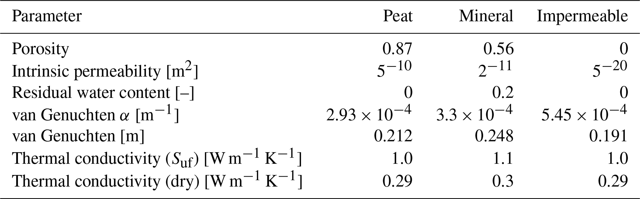
To investigate the effect of freeze–thaw on tracer transport within polygonal tundra, we created idealized transects of high- and low-centered polygons shown in Fig. 1. The 2D transects represent the surface topography and subsurface stratigraphy of our high-centered (left plots) and low-centered (right plots) polygons. We set the diameter of the polygons to be the same, 20 m, which is a representative average value for Arctic polygons (Abolt and Young, 2020). We set the elevation of the center of the high-centered polygon 1.25 m above the trough. We set the top of the low-centered polygon rim 50 cm above its center, based on observations at the BEO site. In both setup cases, the subsurface stratigraphy consists of a peat soil layer overlying a mineral soil layer. In the freeze–thaw-disabled case, we used an additional impermeable layer that represents permafrost. The distance between the ground surface and the impermeable layer represents the active layer and equals 50 cm. In the low-centered polygon, the depth of the peat layer is approximately 10 cm thick in the center of the polygon and 16 cm thick near the troughs. In the high-centered polygon transect, the depth of the peat layer is uniform and equal to 10 cm. This soil stratigraphy represents the general soil stratigraphy that can be commonly found in polygonal tundra in the Arctic coastal plain around the BEO. The hydrothermal properties for each soil layer were previously calibrated for an ice-wedge polygon at the BEO site and are presented in Table 1 (Jan et al., 2020).
Table 1Subsurface thermal properties used for low- and high-centered polygons (from Jan et al., 2020).
To initialize the ATS model for the freeze–thaw-enabled setup, we followed a standard procedure described and implemented in previous studies (Atchley et al., 2015; Jafarov et al., 2018; Jan et al., 2020). This setup includes the following steps: (1) initialize the water table, (2) introduce the energy equation to establish antecedent permafrost as well as initial ice distribution in the domain, and (3) spin up the model with the smoothed meteorological data (Jafarov et al., 2020; Jafarov and Svyatsky, 2021). The spin-up is complete when the model achieves a cyclically stable active layer, in other words, when variations in yearly ground temperatures are insignificant. We set the bottom boundary to a constant temperature of ∘C and set no-flow energy boundary conditions on all other boundaries except the top boundary. For both types of polygon, a seepage flow boundary condition was prescribed 4 cm below the ground surface on the lateral boundaries of the subsurface domain to allow discharge. These boundary conditions allow water to leave the domain and drain to the trough network. The final stage of the spin-up procedure was a 10-year simulation of the integrated surface/subsurface hydrothermal model coupled with the surface energy balance and snow distribution model. We used simplified meteorological data to calculate the surface energy balance, which include a sinusoidally varying air temperature and humidity, constant precipitation, constant radiative forcing, and constant wind. During the thaw season, air temperatures remain above 0 ∘C. In our simulations, we used a simple, sinusoidal temperature time series where the thaw season is 100 d. We applied the tracer 20 d after the first thaw season started at the surface of the polygon within a 2 m radius around the polygon center. Here we consider only advective transport. The total mass of tracer injected into the ground was 25.92 mol. The tracer transport occurs within the surface and subsurface domains, which are coupled via interface tracer fluxes to guarantee the conservation of tracer mass. We assume that the tracer does not mix or become entrapped within ice, so the tracer only resides within the liquid phase.
The freeze–thaw-disabled setup was more straightforward and did not include step 2 mentioned in the above paragraph. First, the initial water table level was established by solving the steady-state variably saturated flow problem. Then we ran the hydrothermal model with an atmospheric temperature of 3 ∘C for 10 years. We performed the freeze–thaw-disabled simulations by setting the layer of soil assumed to be permafrost (i.e., annual temperature below 0 ∘C) to be impermeable. The depth of the impermeable layer was consistent with the active layer depth for the freeze–thaw-enabled condition. The hydrological and thermal parameters used for the peat and the mineral soil layer were the same for the freeze–thaw-disabled and freeze–thaw-enabled setups (Table 1). We ran this case only during the thaw season, approximating the dynamics of the active layer as a step function. In other words, the entire active layer is thawed instantaneously in the spring and refreezes instantaneously in the fall. In this setup, at the beginning of the second thaw season we use model outputs from the end of the first thaw season. This setup is not intended to be physical but is representative of how many hydrothermal permafrost simulations are currently conducted. This setup provides a baseline against which the more physical representation of the freeze–thaw-enabled case can be compared.
In general, it can take from several days to weeks or more from the onset of freezing before the active layer fully freezes, and, in some cases, it never does fully freeze (Cable et al., 2016). The tracer becomes immobile after the freeze-up period. Therefore, the time after freeze-up until the next thaw season has no effect on tracer transport. To demonstrate the effect of the freeze-up on the tracer movement, we calculated the fraction of the tracer mass flux that moves within the active layer during freeze-up. We define the beginning of the freeze-up period as the time when the ground surface starts to freeze, encapsulating warmer ground within the active layer in between the frozen top and the bottom of the active layer.
Our simulations showed enhanced lateral transport in the freeze–thaw-enabled case relative to the freeze–thaw-disabled case. In Fig. 2, we show the difference between simulated tracer flow for the freeze–thaw-disabled and freeze–thaw-enabled cases for the high-centered polygon at the end of the first and second thaw seasons. After the first year, the tracer in the freeze–thaw-disabled case has almost a similar spread to the freeze–thaw-enabled case in general (Fig. 2a and b). After the second year, the tracer amount is lower in the freeze–thaw-enabled case as more tracer has left the center due to lateral transport to the troughs (Fig. 2c and d).
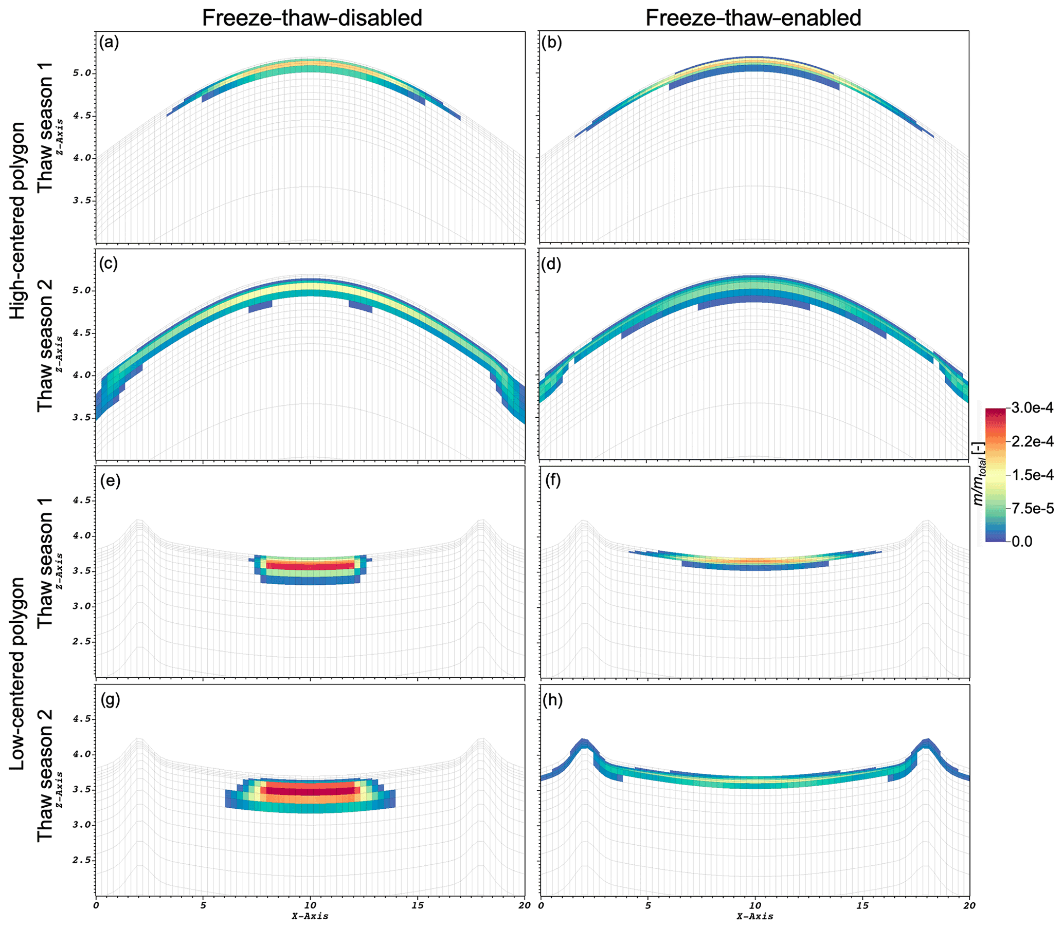
Figure 2Snapshots of the tracer simulation for the freeze–thaw-disabled (a, c, e, g) and freeze–thaw-enabled (b, d, f, h) cases for the high-centered polygon. The top four plots are for the high-centered polygon, and the bottom four are for the low-centered polygon. The first row (a, b) and the third row (e, f) indicate the end of the first thaw season, and the second row (c, d) and the fourth row (g, h) indicate the end of the second thaw season. The color bar represents the fraction of tracer mass with respect to the total mass injected. Here we do not show for values less than 10
The low-centered polygon simulations showed even more dramatic differences between the freeze–thaw-disabled and freeze–thaw-enabled cases than occurred for the high-centered polygon simulations. For the low-centered polygon freeze–thaw-disabled case, more tracer remained in the center of the polygon and vertical transport dominated with little lateral transport (Fig. 2e). By the end of the second thaw season, the tracer propagated even deeper (Fig. 2g). In contrast to the freeze–thaw-disabled case, the enabled case showed significant lateral transport by the end of the first thaw season (Fig. 2f), and by the end of the second thaw season, the differences in lateral versus vertical transport between the two cases were dramatic (Fig. 2g and h).
To quantify the annual tracer flow rates at different locations from the center of the polygon, we calculated the total tracer mass flow rates (Ftotal) within the active layer for years 1 and 2 (Fig. 3). First, we integrated flow rates over the vertical line (face) orthogonally intercepting the polygonal domain and then integrate those values over a whole year. In the freeze–thaw-enabled case, the low-centered polygon shows tracer mobility at up to a 6 m distance from the center for year 1 and full mobility throughout the polygon for year 2 (Fig. 3a). However, the freeze–thaw-disabled case is relatively immobile in comparison, with transport primarily restricted to within 2 m of the polygon center, which is consistent with Fig. 2e and g. In the freeze–thaw-enabled case, the high-centered polygon shows tracer mobility greater than 6 m from the center of the polygon for year 1 and full mobility throughout the polygon for year 2. The freeze–thaw-disabled case shows similar tracer mobility to the enabled case for year 1 and much higher mobility for year 2. The tracer is more mobile within a 6 m distance of the center of the polygon but does not reach the trough even during the second thaw season (Fig. 3b) and shows almost no mobility in the distance from 8 to 10 m. Correspondingly, in Fig. 2c, at the end of thaw season 2, there are close to zero concentrations on the sides of the polygon.

Figure 3The total flow rate (Ftotal) represents the tracer flow rates integrated over the vertical cross-section of the polygon and over the entire year at different distances from the center of the (a) low-centered and (b) high-centered polygon. The proportion of tracer flow rate during the freeze-up period relative to the total flow rate at different distances from the center of the (c) low-centered and (d) high-centered polygon. Ffreezeup represents the tracer flow rates integrated over the vertical cross-section of the polygon and over the freeze-up period at different distances from the center. The solid red curve corresponds to the year 1 and the solid blue corresponds to the year 2 total flow rates for the freeze–thaw-enabled case. The dashed red curve corresponds to year 1 and the dashed blue corresponds to year 2 total flow rates for the freeze–thaw-disabled case.
In our simulation, the freeze-up period lasts less than 2 weeks. To illustrate the amount of the tracer moved through the active layer during the freeze-up period, we calculated the tracer flow rate value during the freeze-up period and divided it by the total flow rate value shown in Fig. 3a and b. The proportion of tracer flow rate during the freeze-up period relative to the annual flow rate is shown in Fig. 3c and d (when the annual flow rate was greater than 0.001 of tracer mass per year). Between 5 % and 40 % of the tracer moved through the active layer during freeze-up during the first thaw season for the low-centered polygon (Fig. 3c). The freeze-up fluxes for year 1 for the high-centered polygon were less than 10 %. During the second year, the freeze-up proportion of transport was less than 10 % in both polygons (Fig. 3c and d).
In addition to the polygon geometry, subsurface characteristics can have an impact on tracer mobility. Advective tracer transport is governed by the porosity and permeability of the soil material. So, we further tested tracer mobility by reducing porosities and permeabilities for the peat and mineral soil layers for the freeze–thaw-enabled case for the low- and high-centered polygonal tundra configurations. Figure 4 corresponds to the reduced-porosity case. To differentiate between different cases, we refer to the cases shown in Figs. 2 and 3 as the base cases. The annual mass flux simulated for the low-centered polygon (Fig. 4a) showed similar dynamics to the base case (Fig. 3c) with a slightly higher mass flux. The annual mass flux simulated for the high-centered polygon (Fig. 4b) showed 2 times the mass flux during year 1 and more mass flux toward the trough of the polygon for year 2 compared to its base case (Fig. 3d). As expected, lower porosity reduces storage and therefore increases transport. The corresponding tracer flux during the freeze-up period is reduced by nearly a factor of 2 for both low- and high-centered polygons (Fig. 4c and d) compared to their respective base case scenarios (Fig. 3c and d, respectively).
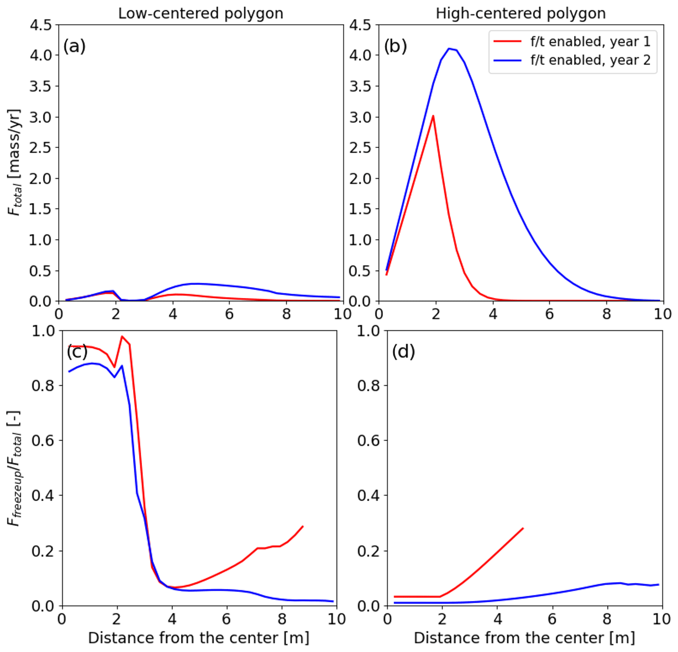
Figure 4The low-porosity setup. The total flow rate (Ftotal) represents the tracer flow rates integrated over the vertical cross-section of the polygon and over the entire year at different distances from the center of the (a) low-centered and (b) high-centered polygon. The proportion of tracer flow rate during the freeze-up period relative to the total flow rate at different distances from the center of the (c) low-centered and (d) high-centered polygon. Ffreezeup represents the tracer flow rates integrated over the vertical cross-section of the polygon and over the freeze-up period at different distances from the center.
For the low-centered polygon, reducing soil permeability by a factor of 10 resulted in a substantial impact on the tracer mobility, leading to reduced annual tracer fluxes (Fig. 5a). The comparison between the low-permeability run (Fig. 5a) and the corresponding base case run (Fig. 3c) indicates a more than 10 times reduction in tracer mobility. The annual mass flux simulated for the high-centered polygon (Fig. 5b) was several magnitudes smaller during year 1, and flux was negligible for year 2. For the low-centered polygon, most of the tracer flux occurred during the freeze-up period, suggesting that freeze-up could be a major mechanism moving tracer in low-permeability soils. For the high-centered polygon, the tracer fluxes simulated during the freeze-up period showed 3 times more flux for year 2 than similar fluxes simulated for the base case scenario (Figs. 5d and 3d).

Figure 5The low-permeability setup. The total flow rate (Ftotal) represents the tracer flow rates integrated over the vertical cross-section of the polygon and over the entire year at different distances from the center of the (a) low-centered and (b) high-centered polygon. The proportion of tracer flow rate during the freeze-up period relative to the total flow rate at different distances from the center of the (c) low-centered and (d) high-centered polygon. Ffreezeup represents the tracer flow rates integrated over the vertical cross-section of the polygon and over the freeze-up period at different distances from the center.
4.1 Polygon geometry
The field experiment of Wales et al. (2020) suggests tracer movement during the freeze-up period. We can see that the tracer movement during the freeze-up period is more pronounced for the low-centered polygon (Fig. 3c). Differences in high-centered and low-centered freeze-up effects are likely primarily due to geomorphological differences where the geometry of the polygon dictates the flow of heat (Abolt et al., 2018). For example, high-centered polygons freeze from the center (because it is the highest and most exposed region) and troughs stay warmer. In contrast, the centers of the low-centered polygons stay warmer than their sides due to the cooling effect of their elevated rims (Abolt et al., 2018). Cooler rims should allow water movement toward them. In both cases, during the first year, the freeze-up contributions are greater at the rims and troughs than in the center. This fact explains the wider spread of the tracer for the freeze–thaw-enabled cases. To further test the influence of the polygon geometry, we set up a similar tracer experiment using a flat-centered polygon. Figure 6a shows that simulated annual flow rates for a flat-centered polygon are smaller than similar fluxes for the high- and low-centered polygons. The annual flow rates suggest that no tracer or a very small amount of tracer reaches the trough. The freeze–thaw-enabled case, however, moves more tracer than the freeze–thaw-disabled case for the high-centered polygon. This additional experiment with the flat-centered polygon shows the importance of the polygon geometry for the tracer movement within the active layer.
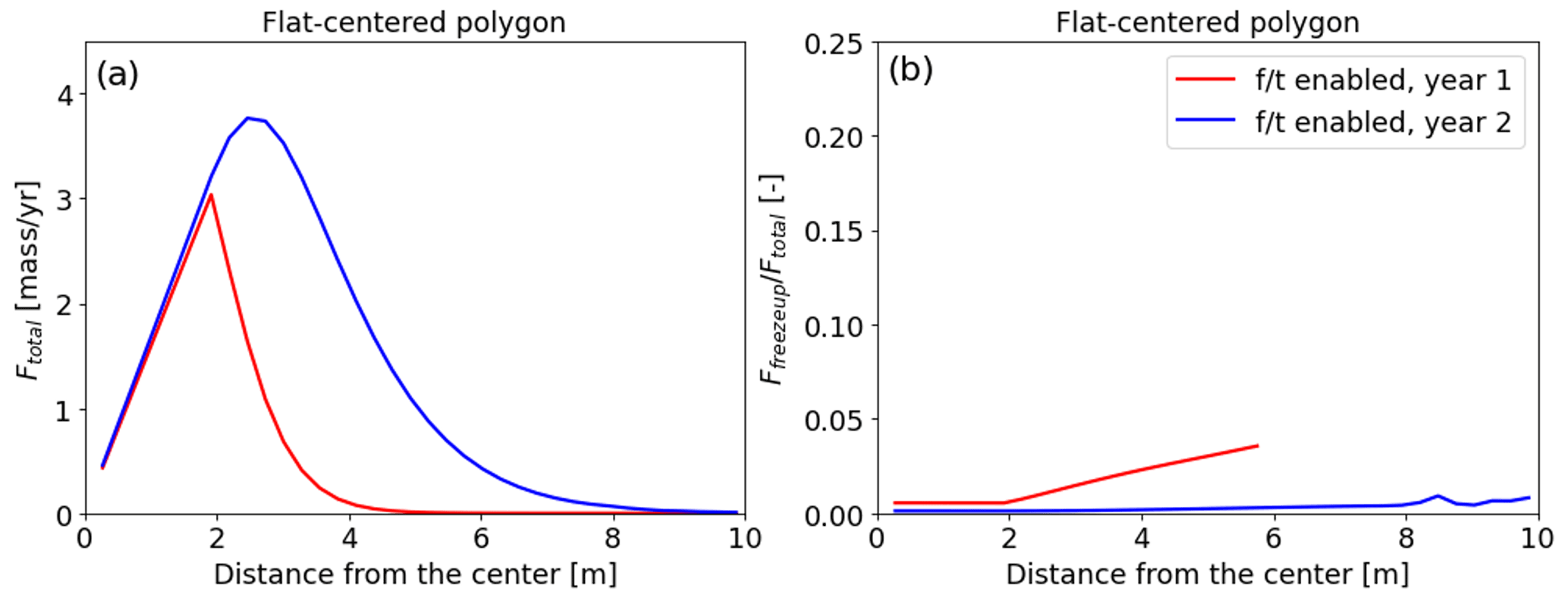
Figure 6(a) The total flow rate (Ftotal) represents the tracer flow rates integrated over the vertical cross-section of the flat-centered polygon and over the entire year at different distances from the center. (b) The proportion of tracer flow rate during the freeze-up period relative to the total flow rate at different distances from the center of the flat-centered polygon. Ffreezeup represents the tracer flow rates integrated over the vertical cross-section of the flat-centered polygon and over the freeze-up period at different distances from the center.
4.2 Subsurface characteristics
The freeze-up impacts tracer transport as a result of thinning of the unfrozen space between the top and bottom freezing fronts of the active layer, pushing tracer further to the sides. The polygon geometry and subsurface characteristics could amplify or reduce the freeze-up impact. For example, low-centered polygon geometry allows more tracer transport than flat-centered geometry under the same meteorological inputs. On the other hand, tracer mobility depends on subsurface permeability and porosity characteristics, slowing down or accelerating tracer transport. We showed that reducing porosity and permeability reduces tracer mobility, amplifying the impact of freeze-up and suggesting that closing freezing fronts push more tracer during freeze-up. This effect could be a result of the Clausius–Clapeyron equation when liquid is pushed from thawed to frozen parts of the ground, described by Davis (2001).
Our results illustrate the importance of hydraulic and thermal gradients. The impact of hydraulic gradients plays an essential role for the high-centered polygons. The freeze–thaw-disabled case (Fig. 2a and c) confirms the strong influence of hydraulic gradients between the center and troughs of the high-centered polygon, providing almost similar tracer mobility to that simulated for the freeze–thaw-enabled case. Inversely, thermal gradients move tracer in the case of the low-centered polygon, indicating that without thermal gradients, the tracer stays immobile (Fig. 2e and g).
4.3 Experimental study
In the experiment conducted by Wales et al. (2020), tracer concentration dropped for year 2 and did not resume where it had ended in the previous year. Most of the tracer that had traveled vertically over the first year reached the bottom of the active layer. The mobility did not resume until the end of the second thaw season when the active layer was at its maximum depth. Similar behavior was exhibited by the simulated tracer. In the field experiment, the heterogeneous active layer depth within the actual polygon could lead to different pathways found by the tracer and further tracer distribution and overall dilution. Our numerical experiment is more representative of the ideal lab experiment than the actual field study and, therefore, not directly comparable with the complex conditions in the field. The main objective of these simulations was not to replicate the field experiment of Wales et al. (2020) because those experiments were conducted on two specific polygons and the field polygon sizes, geometries, stratigraphies, moisture content conditions, etc. do not always correspond to the generalized parameterizations used in the simulations. However, it is worth examining similarities and differences of the field study and the simulations from at least a conceptual viewpoint.
Both field studies and simulations showed the consistent freeze-up effect. The largest difference between the simulations and the field tracer results is that the simulations suggest greater transport in high-centered polygons than low-centered polygons, while the field tracer study indicated the opposite. Wales et al. (2020) suggested that the continuously saturated conditions in the low-centered polygon (and sometimes ponded surface water conditions) led to greater transport in the low-centered polygon. In contrast, the top of the high-centered polygon where the field tracer was applied was frequently unsaturated. A future coordinated field and modeling approach would be needed to better constrain transport differences related to polygon types and to refine the simulation approach. The simulations and the field tracer study are consistent in showing that polygon-center-to-trough lateral transport occurs and that freeze-up effects are important, and both the simulations and field experiments show that transport needs to be assessed on a multi-year or multi-thaw season timeframe. We define the breakthrough condition to be when the flux at a specific location is not zero. The simulations and the field tests indicate that more than 2 years is needed for a full breakthrough of the tracer mass to the trough, and the overall residence time of the tracer in the polygon is likely quite prolonged, requiring many more thaw seasons. This multi-year timeframe has important implications in terms of actual carbon exports from polygon centers to troughs and likely has substantial effects on biogeochemical conditions, which have been shown to be quite different between polygon centers and troughs (e.g., Newman et al., 2015; Wainwright et al., 2015).
For the low-centered polygon simulations, the differences between the freeze–thaw-disabled and freeze–thaw-enabled cases were more substantial (e.g., Figs. 2e–h and 3a). The freeze–thaw-disabled case showed no trough breakthrough over the 2-year simulation period and the freeze–thaw-enabled case showed breakthrough in year 2. The field tracer study showed breakthrough in year 1. However, Wales et al. (2020) suggested that this was likely a preferential flow effect which was not considered in the simulations. The freeze-up for the low-centered polygon case only showed a small amount of tracer mass reaching the trough, which is qualitatively consistent with the overall low breakthrough mass observed in the field tracer study.
4.4 Cryosuction
One of the key transport considerations during the freeze-up period is cryosuction. During this process, water is drawn toward the freezing front due to capillary forces, a phenomenon that the freeze–thaw-enabled simulations include but the freeze–thaw-disabled simulations do not (Painter and Karra, 2014). In the freeze–thaw-enabled case simulations, substantial impacts on low-centered polygon transport were observed, consistent with the pre- and post-freeze-up observations of Wales et al. (2020) and supporting their assertion that freeze-up effects may be responsible for further tracer transport. For the high-centered polygon, differences between the freeze–thaw-disabled and freeze–thaw-enabled cases were smaller, suggesting that freeze-up effects were not as important. Apparent freeze-up effects were observed for the high-centered polygon in the field tracer study, but it was difficult to ascertain whether these effects were less pronounced than in the low-centered polygon. Our numerical study illustrates the importance of the freeze–thaw dynamics for the mobility of tracer in polygonal tundra. In some years, the freeze-up period might extend into the late fall due to snowfall and the subsequent subsurface conditions (Cable et al., 2016; Jan and Painter, 2020). An extended freeze-up period would further increase tracer movement within a given year, and the multi-year duration for full tracer breakthrough discussed above means that transport would be affected by multiple freeze-up periods. The importance of freeze-up effects for transport may extend beyond polygon areas, affecting a broad range of permafrost landscapes during active layer freezing, and further fieldwork and modeling work are warranted to characterize freeze–thaw effects on these other landscapes.
4.5 Implications
Monitored ground temperatures in Alaska indicate significant warming over the last 30 years (Wang et al., 2018). Such warming would suggest active layer thickening; however, ground subsidence counteracts the effect of increased temperature on active layer thickness (Streletskiy et al., 2017). Subsidence has hydrological effects due to soil compaction, which increases bulk density, and thaw can release previously frozen soil carbon even though the apparent active layer thickness does not increase (Jorgenson and Osterkamp, 2005; Plaza et al., 2019). Lateral transport of this carbon would cause redistribution, potentially affecting local carbon stocks and redox conditions which would affect microbial carbon dioxide and methane production. Accounting for lateral carbon transport in watershed-scale to earth-system-scale models would help decrease current uncertainties associated with tundra carbon dynamics. The significance of lateral subsurface transport is highlighted by Plaza et al. (2019), who suggest that more than half of soil carbon loss may be associated with lateral flow. Improved accounting of tundra organic carbon loss can clarify ecosystem source–sink relations and how they may change with additional permafrost degradation. This study shows that lateral subsurface transport (of carbon and other dissolved constituents) from polygon centers to troughs is important over multi-year timeframes and that transport during the freeze-up period should be represented in models of these systems, especially in the case of low-centered polygons.
The numerical experiments we conducted in this study illustrate the importance of polygon geometry and the freeze–thaw cycle for subsurface transport. In particular, we showed how hydraulic and thermal gradients act on high- and low-centered polygons. For a high-centered polygon, hydraulic gradients are the main drivers of the subsurface water flow. The freeze–thaw-disabled and freeze–thaw-enabled cases showed almost similar tracer mobility. For a low-centered polygon, hydraulic gradients allow only vertical tracer movement; the convex shape of the polygon leads to tracer immobility when thermal gradients are not included. For a low-centered polygon, thermal gradients provide a substantial force in moving tracer to the troughs.
We tested a hypothesis postulated by Wales et al. (2020), suggesting that freeze-up could promote additional tracer movement in the active layer of the low- and high-centered polygon. In all freeze–thaw-enabled cases, we observed a consistent freeze-up effect extending tracer mobility until complete active layer freeze-up. In the current simulations, the freeze-up period is no longer than 2 weeks, whereas most of the tracer is transported over the thaw season. However, longer freeze-up times could promote further tracer mobility.
The ATS is a collection of representations of physical processes designed to work within a flexibly configured modeling framework (Coon et al., 2019). This modeling framework is a powerful multiphysics simulator designed on the basis of the Arcos management system. In this study, we coupled the surface and subsurface thermo-hydrology and surface energy balance components of the ATS (Atchley et al., 2015; Painter et al., 2016; Jafarov et al., 2018) with a non-reactive transport model. This configuration of the ATS is an integrated thermo-hydrologic model including a surface energy balance, enabling the simulation of snowpack evolution, surface runoff, and subsurface flow in the presence of phase change. The entire system is mass and energy conservative and is forced by meteorological data and appropriate initial and boundary conditions.
The surface energy balance model uses incoming and outgoing radiation, latent and sensible heat exchange, and diffusion of energy to the soil to determine a snowpack temperature and simulate the evolution of the snowpack (Atchley et al., 2015). The snowpack evolution model includes snow aging, density changes, and depth hoar and, based on subsurface conditions, determines energy fluxes between the surface and subsurface. Overland flow is modeled using the diffusion wave approximation, which is derived based on Manning's surficial roughness coefficient, with modifications to account for frozen surface water. Additionally, transport of energy on the surface is tracked through an advection–diffusion transport equation that supports phase changes.
Subsurface thermal hydrology is represented in the ATS by a modified Richards' equation coupled to an energy equation. Unfrozen water at temperatures below 0 ∘C, an important physical phenomenon for accurate modeling of permafrost (e.g., Romanovsky and Osterkamp, 2000), is represented through a constitutive relation (Painter and Karra, 2014) based on the Clapeyron equation, which partitions water into the three phases. Density changes associated with phase change and cryosuction (i.e., the “freezing equals drying” approximation) are included. Karra et al. (2014) demonstrated that this formulation is able to reproduce several variably saturated, freezing soil laboratory experiments without resorting to empirical soil freezing curves or impedance factors in the relative permeability model.
Other key constitutive equations for this model include a water retention curve, here the van Genuchten–Mualem formulation (van Genuchten, 1980; Mualem, 1976), and a model for thermal conductivity of the air–water–ice–soil mixture. The method for calculating thermal conductivities of the air–water–ice–soil mixture is based on interpolating between saturated frozen, saturated unfrozen, and fully dry states (Painter et al., 2016), where the thermal conductivities of each end-member state are determined by the thermal conductivity of the components (soil grains, air, water, or liquid) weighted by the relative abundance of each component in the cell (Johansen, 1977; Peters-Lidard et al., 1998; Atchley et al., 2015). Standard empirical fits are used for the internal energy of each component of the air–water–ice–soil mixture.
The Advanced Terrestrial Simulator (ATS) (Coon et al., 2019) is open source under the BSD 3-clause license, and is publicly available at https://github.com/amanzi/ats (last access: 8 March 2022). Simulations were conducted using version 1.2.0.
The dataset that includes all the ATS input and visualization scripts used in this study is documented in Jafarov and Svyatsky (2021, https://doi.org/10.5440/1764110).
EJ and DS were responsible for the study design and analysis. DS was responsible for the numerical simulation setup, model runs, and results processing. EJ, DS, and BN drafted the manuscript. EJ, DS, BN, and DH edited and revised the manuscript. DM and CW provided support and leadership.
The contact author has declared that neither they nor their co-authors have any competing interests.
Publisher's note: Copernicus Publications remains neutral with regard to jurisdictional claims in published maps and institutional affiliations.
This work is part of the Next-Generation Ecosystem Experiments (NGEE Arctic) project which is supported by the Office of Biological and Environmental Research in the DOE Office of Science.
This research has been supported by the Office of Science (NGEE Arctic grant).
This paper was edited by Ylva Sjöberg and reviewed by two anonymous referees.
Abolt, C. J. and Young, M. H.: High-resolution mapping of spatial heterogeneity in ice wedge polygon geomorphology near Prudhoe Bay, Alaska, Sci. Data, 7, 87, https://doi.org/10.1038/s41597-020-0423-9, 2020.
Abolt, C. J., Young, M. H., Atchley, A. L., and Harp, D. R.: Microtopographic control on the ground thermal regime in ice wedge polygons, The Cryosphere, 12, 1957–1968, https://doi.org/10.5194/tc-12-1957-2018, 2018.
Andresen, C. G., Lawrence, D. M., Wilson, C. J., McGuire, A. D., Koven, C., Schaefer, K., Jafarov, E., Peng, S., Chen, X., Gouttevin, I., Burke, E., Chadburn, S., Ji, D., Chen, G., Hayes, D., and Zhang, W.: Soil moisture and hydrology projections of the permafrost region – a model intercomparison, The Cryosphere, 14, 445–459, https://doi.org/10.5194/tc-14-445-2020, 2020.
Atchley, A. L., Painter, S. L., Harp, D. R., Coon, E. T., Wilson, C. J., Liljedahl, A. K., and Romanovsky, V. E.: Using field observations to inform thermal hydrology models of permafrost dynamics with ATS (v0.83), Geosci. Model Dev., 8, 2701–2722, https://doi.org/10.5194/gmd-8-2701-2015, 2015.
Cable, W. L., Romanovsky, V. E., and Jorgenson, M. T.: Scaling-up permafrost thermal measurements in western Alaska using an ecotype approach, The Cryosphere, 10, 2517–2532, https://doi.org/10.5194/tc-10-2517-2016, 2016.
Coon, E., Svyatsky, D., Jan, A., Kikinzon, E., Berndt, M., Atchley, A., Harp, D., Manzini, G., Shelef, E., Lipnikov, K., Garimella, R., Xu, C., Moulton, D., Karra, S., Painter, S., Jafarov, E., and Molins, S.: Advanced Terrestrial Simulator, Los Alamos National Laboratory (LANL), Los Alamos, NM (United States), https://doi.org/10.11578/DC.20190911.1, 2019.
Corapcioglu, M. Y. and Sorab, P.: Thawing permafrost – simulation and verification, in: Permafrost Fifth International Conference, 1988.
Davis, T. N.: Thawing permafrost – simulation and verification, Permafrost Fifth International Conference, Proceeding Volume 1, 2–5 August, 351 pp., 2001.
Frampton, A. and Destouni, G.: Impact of degrading permafrost on subsurface solute transport pathways and travel times, Water Resour. Res., 51, 7680–7701, https://doi.org/10.1002/2014WR016689, 2015.
Hinzman, L. D., Johnson, R. A., Kane, D. L., Farris, A. M., and Light, G. J.: Measurements and modeling of benzene transport in a discontinuous permafrost region, in: Contaminant Hydrology, CRC Press, ISBN 1-889963-19-4, 175–237, 2000.
Jafarov, E. and Svyatsky, D.: The Importance of Freeze/Thaw Cycles on Lateral Transport in Ice-Wedge Polygons: Modeling Archive. Next Generation Ecosystem Experiments Arctic Data Collection, Oak Ridge National Laboratory, U.S. Department of Energy, Oak Ridge, Tennessee, USA [data set], https://doi.org/10.5440/1764110, 2021.
Jafarov, E. E., Coon, E. T., Harp, D. R., Wilson, C. J., Painter, S. L., Atchley, A. L., and Romanovsky, V. E.: Modeling the role of preferential snow accumulation in through talik development and hillslope groundwater flow in a transitional permafrost landscape, Environ. Res. Lett., 13, 105006, https://doi.org/10.1088/1748-9326/aadd30, 2018.
Jafarov, E. E., Harp, D. R., Coon, E. T., Dafflon, B., Tran, A. P., Atchley, A. L., Lin, Y., and Wilson, C. J.: Estimation of subsurface porosities and thermal conductivities of polygonal tundra by coupled inversion of electrical resistivity, temperature, and moisture content data, The Cryosphere, 14, 77–91, https://doi.org/10.5194/tc-14-77-2020, 2020.
Jan, A. and Painter, S. L.: Permafrost thermal conditions are sensitive to shifts in snow timing, Environ. Res. Lett., 15, 084026, https://doi.org/10.1088/1748-9326/ab8ec4, 2020.
Jan, A., Coon, E. T., and Painter, S. L.: Evaluating integrated surface/subsurface permafrost thermal hydrology models in ATS (v0.88) against observations from a polygonal tundra site, Geosci. Model Dev., 13, 2259–2276, https://doi.org/10.5194/gmd-13-2259-2020, 2020.
Johansen, O.: Thermal Conductivity of Soils, Cold regions research and engineering lab Hanover NH, 1977.
Jorgenson, M. T. and Osterkamp, T. E.: Response of boreal ecosystems to varying modes of permafrost degradation, Can. J. For. Res., 35, 2100–2111, https://doi.org/10.1139/x05-153, 2005.
Karra, S., Painter, S. L., and Lichtner, P. C.: Three-phase numerical model for subsurface hydrology in permafrost-affected regions (PFLOTRAN-ICE v1.0), The Cryosphere, 8, 1935–1950, https://doi.org/10.5194/tc-8-1935-2014, 2014.
Liljedahl, A. K., Boike, J., Daanen, R. P., Fedorov, A. N., Frost, G. V., Grosse, G., Hinzman, L. D., Iijma, Y., Jorgenson, J. C., Matveyeva, N., Necsoiu, M., Raynolds, M. K., Romanovsky, V. E., Schulla, J., Tape, K. D., Walker, D. A., Wilson, C. J., Yabuki, H., and Zona, D.: Pan-Arctic ice-wedge degradation in warming permafrost and its influence on tundra hydrology, Nat. Geosci., 9, 312–318, https://doi.org/10.1038/ngeo2674, 2016.
McGuire, A. D., Lawrence, D. M., Koven, C., Clein, J. S., Burke, E., Chen, G., Jafarov, E., MacDougall, A. H., Marchenko, S., Nicolsky, D., Peng, S., Rinke, A., Ciais, P., Gouttevin, I., Hayes, D. J., Ji, D., Krinner, G., Moore, J. C., Romanovsky, V., Schädel, C., Schaefer, K., Schuur, E. A. G., and Zhuang, Q.: Dependence of the evolution of carbon dynamics in the northern permafrost region on the trajectory of climate change, P. Natl. Acad. Sci. USA, 115, 3882–3887, https://doi.org/10.1073/pnas.1719903115, 2018.
Mualem, Y.: A new model for predicting the hydraulic conductivity of unsaturated porous media, Water Resour. Res., 12, 513–522, https://doi.org/10.1029/WR012i003p00513, 1976.
Newman, B. D., Throckmorton, H. M., Graham, D. E., Gu, B., Hubbard, S. S., Liang, L., Wu, Y., Heikoop, J. M., Herndon, E. M., Phelps, T. J., Wilson, C. J., and Wullschleger, S. D.: Microtopographic and depth controls on active layer chemistry in Arctic polygonal ground, Geophys. Res. Lett., 42, 1808–1817, https://doi.org/10.1002/2014GL062804, 2015.
O'Donnell, J., Douglas, T., Barker, A., and Guo, L.: Changing Biogeochemical Cycles of Organic Carbon, Nitrogen, Phosphorus, and Trace Elements in Arctic Rivers, in: Arctic Hydrology, Permafrost and Ecosystems, edited by: Yang, D. and Kane, D. L., Springer International Publishing, Cham, 315–348, https://doi.org/10.1007/978-3-030-50930-9_11, 2021.
Painter, S. L. and Karra, S.: Constitutive Model for Unfrozen Water Content in Subfreezing Unsaturated Soils, Vadose Zone J., 13, vzj2013.04.0071, https://doi.org/10.2136/vzj2013.04.0071, 2014.
Painter, S. L., Coon, E. T., Atchley, A. L., Berndt, M., Garimella, R., Moulton, J. D., Svyatskiy, D., and Wilson, C. J.: Integrated surface/subsurface permafrost thermal hydrology: Model formulation and proof-of-concept simulations: Integrated permafrost thermal hydrology, Water Resour. Res., 52, 6062–6077, https://doi.org/10.1002/2015WR018427, 2016.
Peters-Lidard, C. D., Blackburn, E., Liang, X., and Wood, E. F.: The Effect of Soil Thermal Conductivity Parameterization on Surface Energy Fluxes and Temperatures, J. Atmos.Sci., 55, 1209–1224, https://doi.org/10.1175/1520-0469(1998)055<1209:TEOSTC>2.0.CO;2, 1998.
Plaza, C., Pegoraro, E., Bracho, R., Celis, G., Crummer, K. G., Hutchings, J. A., Hicks Pries, C. E., Mauritz, M., Natali, S. M., Salmon, V. G., Schädel, C., Webb, E. E., and Schuur, E. A. G.: Direct observation of permafrost degradation and rapid soil carbon loss in tundra, Nat. Geosci., 12, 627–631, https://doi.org/10.1038/s41561-019-0387-6, 2019.
Raisbeck, J. M. and Mohtadi, M. F.: The environmental impacts of oil spills on land in the arctic regions, Water Air Soil Pollut., 3, 195–208, https://doi.org/10.1007/BF00166630, 1974.
Romanovsky, V. E. and Osterkamp, T. E.: Effects of unfrozen water on heat and mass transport processes in the active layer and permafrost, Permafr. Periglac., 11, 219–239, https://doi.org/10.1002/1099-1530(200007/09)11:3<219::AID-PPP352>3.0.CO;2-7, 2000.
Strauss, J., Schirrmeister, L., Grosse, G., Wetterich, S., Ulrich, M., Herzschuh, U., and Hubberten, H.-W.: The deep permafrost carbon pool of the Yedoma region in Siberia and Alaska, Geophys. Res. Lett., 40, 6165–6170, https://doi.org/10.1002/2013GL058088, 2013.
Streletskiy, D. A., Shiklomanov, N. I., Little, J. D., Nelson, F. E., Brown, J., Nyland, K. E., and Klene, A. E.: Thaw Subsidence in Undisturbed Tundra Landscapes, Barrow, Alaska, 1962-2015: Barrow Subsidence, Permafr. Periglac., 28, 566–572, https://doi.org/10.1002/ppp.1918, 2017.
van Genuchten, M. Th.: A Closed-form Equation for Predicting the Hydraulic Conductivity of Unsaturated Soils, Soil Sci. Soc. Am. J., 44, 892–898, https://doi.org/10.2136/sssaj1980.03615995004400050002x, 1980.
Wainwright, H. M., Dafflon, B., Smith, L. J., Hahn, M. S., Curtis, J. B., Wu, Y., Ulrich, C., Peterson, J. E., Torn, M. S., and Hubbard, S. S.: Identifying multiscale zonation and assessing the relative importance of polygon geomorphology on carbon fluxes in an Arctic tundra ecosystem, J. Geophys. Res.-Biogeo., 120, 788–808, https://doi.org/10.1002/2014JG002799, 2015.
Wales, N. A., Gomez-Velez, J. D., Newman, B. D., Wilson, C. J., Dafflon, B., Kneafsey, T. J., Soom, F., and Wullschleger, S. D.: Understanding the relative importance of vertical and horizontal flow in ice-wedge polygons, Hydrol. Earth Syst. Sci., 24, 1109–1129, https://doi.org/10.5194/hess-24-1109-2020, 2020.
Wang, K., Jafarov, E., Overeem, I., Romanovsky, V., Schaefer, K., Clow, G., Urban, F., Cable, W., Piper, M., Schwalm, C., Zhang, T., Kholodov, A., Sousanes, P., Loso, M., and Hill, K.: A synthesis dataset of permafrost-affected soil thermal conditions for Alaska, USA, Earth Syst. Sci. Data, 10, 2311–2328, https://doi.org/10.5194/essd-10-2311-2018, 2018.