the Creative Commons Attribution 4.0 License.
the Creative Commons Attribution 4.0 License.
 | 25 Feb 2022
Brief communication: Impact of common ice mask in surface mass balance estimates over the Antarctic ice sheet
Sebastian B. Simonsen
Fredrik Boberg
Christoph Kittel
Andrew Orr
Niels Souverijns
J. Melchior van Wessem
Ruth Mottram
Regional climate models compute ice sheet surface mass balance (SMB) over a mask that defines the area covered by glacier ice, but ice masks have not been harmonised between models. Intercomparison studies of modelled SMB therefore use a common ice mask. The SMB in areas outside the common ice mask, which are typically coastal and high-precipitation regions, is discarded. Ice mask differences change integrated SMB by between 40.5 and 140.6 Gt yr−1 (1.8 % to 6.0 % of ensemble mean SMB), equivalent to the entire Antarctic mass imbalance. We conclude there is a pressing need for a common ice mask protocol.
- Article
(2242 KB) - Full-text XML
- BibTeX
- EndNote


Detailed estimates of the surface mass balance (SMB) of the Antarctic ice sheet (AIS) are important for interpreting observed ice and sea-level-rise budgets. SMB is the difference between accumulation and ablation at the surface of the ice sheet, which in Antarctica is positive due to the precipitation term dominating, especially in coastal areas, where high relief is often found due to complex/steep orography leading to orographic precipitation (Lenaerts et al., 2019).
Multiple regional climate models (RCMs) are now used to provide estimates of present-day and projected SMB. A selection of five of these were recently the subject of an intercomparison exercise (Mottram et al., 2021) to explore their commonalities and differences. Modelled present-day SMB for the total AIS (ToAIS, which we define as the ice sheet including ice shelves) in the scientific literature ranges from 2177±80 to 2583±122 Gt yr−1 (van Wessem et al., 2018; Souverijns et al., 2019; Agosta et al., 2019; Hansen et al., 2021a). The intercomparison in Mottram et al. (2021) gives an ensemble mean of 2329±94 Gt yr−1 for the common period of 1987 to 2015 with a range of 1961±70 to 2519±118 Gt yr−1 for individual models. Their results also show that while all models vary on an interannual basis directed by the driving ERA-Interim reanalysis, the spread in mean annual SMB estimates originates predominantly from differences in the dynamical core, physical parameterisations, model set-up and the digital elevation model (DEM). Spatial differences in the pattern of SMB can be attributed locally to resolution and differences in orography, but continental-scale variability in the distribution of precipitation is related predominantly to model physics and dynamical cores (Mottram et al., 2021). While all models were able to reproduce observed temperatures, pressures and wind speeds measured at automatic weather stations across the continent, models with nudging or daily reinitialisation had in general smaller biases but even so differing regional patterns of SMB (see e.g. Fig. 4 in Mottram et al., 2021). Comparisons with the limited SMB observations available show that different models perform better in different regions and at different altitudes, making it challenging to draw general conclusions on a continental scale. Although there are multiple reasons for the range in estimates of SMB, we focus solely on the ice masks in this study in order to assess differences in SMB introduced in post-processing of model estimates. The Mottram et al. (2021) intercomparison study used a common ice mask to remove continent-wide present-day SMB differences related to variations in native ice mask extent. Ice masks are typically made up of a binary grid that defines ice-covered areas, including ice shelves, and the ocean.
Here, we aim to quantify the importance of the ice mask in explaining the difference in SMB simulated by the five RCMs used in the Mottram et al. (2021) intercomparison study: COSMO-CLM2 (Souverijns et al., 2019), HIRHAM5 (Hansen et al., 2021a), MARv3.10 (Agosta et al., 2019), MetUM (Orr et al., 2015) and RACMO2.3p2 (van Wessem et al., 2018). We investigate the importance of the different native ice masks by creating a surface categorisation that shows the number of models that are represented in each grid cell. Furthermore, we show the spatial differences on a basin scale induced by the common mask. All the native masks have been regridded onto the same grid at a 0.11∘ (≈12.5 km) resolution.
Usually, SMB estimates over the AIS are confined to the grounded AIS because it is only the mass change over the grounded AIS that results directly in sea-level change (Lenaerts et al., 2019). However, we include the ice shelves in all results due to their buttressing of the main ice sheet and thereby importance for the general ice sheet dynamics (Dupont and Alley, 2005). We also show the integrated ΔSMB for the grounded ice sheet in Table 1. Thinning of the ice shelves has already been observed, which results in less buttressing and increased discharge from the grounded ice into the ocean (Gudmundsson et al., 2019). Further, the largest change in end-of-century-projected AIS surface mass balance is shown to occur over the ice shelves (Kittel et al., 2021); it is therefore an important feature to get right in Antarctic modelling.
The five models were run in the Antarctic domain from 1987 to 2015 at different horizontal spatial resolutions and different land–sea mask data sets: COSMO-CLM2 at a 0.22∘ resolution, with an ice mask created with data from the Scientific Committee on Antarctic Research (SCAR) Antarctic Digital Database version 5.0 published in 2006 (Lawrence et al., 2019); HIRHAM5 at two resolutions of 0.11 and 0.44∘, with an ice mask derived from data created by the United States Geological Survey (USGS) Earth Resources Observation and Science (EROS) Center and consisting of Advanced Very High Resolution Radiometer (AVHRR) data at a 1 km resolution collected from 1992 to 1993 (Eidenshink and Faudeen, 1994); MetUM at a 0.44∘ resolution, which has an ice mask created from the International Geosphere-Biosphere Programme (IGBP) data in combination with 1 km AVHRR data from the period of 1992 to 1993 (Loveland et al., 2000); MARv3.10 at a 0.32∘ resolution, with an ice mask created from Bedmap2, which consists of a combination of different data sources such as satellite images, radar and laser altimetry gathered between 2000 and 2010 (Fretwell et al., 2013); and RACMO2.3p2 at a 0.25∘ resolution, with an ice mask made from a 1 km DEM that was created from the combination of ERS-1 data from 1994 and ICESat data from 2003 to 2008 (Bamber et al., 2009).
Mottram et al. (2021) regridded all native ice masks and SMB estimates to a common grid of 0.11∘. We adopt this approach and refer to Mottram et al. (2021) for details. We then compare the SMB over the common mask and the native ice masks used in each individual original model simulation. The common mask is defined as all points where all the regridded native ice masks have grid cells that are covered with permanent ice. We break the simulated SMB down to the basin scale using Antarctic drainage basins derived from Zwally et al. (2012), including ice shelves (see Fig. 1). Note that the Zwally et al. (2012) basins define an outer edge of the ToAIS; in all cases the native masks are slightly larger than the Zwally et al. (2012) definition. To make the grounded ice sheet values in Table 1, we derived the values of the grounded ice sheet, using the data set for grounded ice from Zwally et al. (2012), since not all the native masks explicitly distinguished grounded from floating ice. This way we insured all the native masks and the common mask were compared equally. In Table 2 we opted to define differences only over the basins defined in Zwally et al. (2012) in order to be consistent with other studies. Both the area and the SMB have been calculated for the common mask and native masks in each of the 27 basins. Three values are given for each model basin: Δarea%, the percentage difference in area; ΔSMB%, the percentage difference in SMB; and ΔSMBGt yr-1, the difference in SMB in Gt yr−1. All calculations are derived by subtracting the regridded native mask from the common mask (Δ = common − native).
Comparing the area of the common mask to the area of the native masks, we see that the common mask is between 1.85 % and 2.89 % smaller than the different native masks (Table 1). This results in integrated SMB values that are between 40.5 and 140.6 Gt yr−1 smaller when using the common mask compared to the native mask, which is up to 6.04 % of the ensemble mean SMB (Mottram et al., 2021) (Table 1). The two HIRHAM5 simulations are very close to having identical areas; however the SMB is larger in the 0.11∘ simulation, which is most likely due to the steep coastal orography being better resolved and thus leading to increased orographic precipitation (Webster et al., 2008). In the rightmost column ΔSMBGt yr-1 over the grounded AIS is shown; when excluding the ice shelves there are still differences between the common mask and the native masks of between 20.1 and 102.4 Gt yr−1 (Table 1). It should be pointed out that a small Δ value is not necessarily more correct than a large Δ value in terms of true area size or SMB magnitude. It solely refers to how close it is to the common mask and the ensemble mean from Mottram et al. (2021).
Table 1From left to right the columns show the RCM name; Δarea% and ΔSMBGt yr-1 – both between the common mask and the native mask over the ToAIS; ΔSMB% – the difference between ΔSMBGt yr-1 and the SMB ensemble mean from Mottram et al. (2021), which is 2329 Gt yr−1, the yearly SMB for the individual models integrated over the common mask with uncertainties of 1 standard deviation; and finally ΔSMBGt yr-1 over the grounded AIS.

The different model–mask combinations are shown in Fig. 1. Around the Antarctic Peninsula (basins 24–27) there are large mask disagreements over the Larsen C ice shelf and at the tip of the peninsula and the surrounding islands. Parts of the West AIS, especially glaciers such as Getz (basin 20), Thwaites (basin 21) and Abbot (basin 23), also have large mask disagreements as do, in the East AIS, places like the Fimbul, Amery and West ice shelves (Fig. 1). All around the coastline we see, going from the ice sheet and out towards the ocean, that the number of ice masks outside the common mask decreases. Furthermore, two of the masks, COSMO-CLM2 and MARv3.10, contain non-iced grid cells in their native masks, simulating some parts of non-ice-covered parts of the Transantarctic Mountains (Fig. 1a). Moreover, it is shown how well the common mask agrees to a newly derived ice mask. We compare the common mask to the Reference Elevation Model of Antarctica (REMA; Howat et al., 2019) mask over the Antarctic Peninsula (AP); here it is clear that the common mask is smaller than REMA in most coastal areas around the AP (Fig. 1b).

Figure 1Panel (a) shows the ice mask agreement; the white area is the common mask (i.e. where all six masks have ice), and the colours around the coastline represents the number of native masks that have ice outside the common mask. The numbers refer to the 27 drainage basins with ice shelves, outlined in turquoise, and IS is short for ice shelf and AP, WAIS and EAIS are the Antarctic Peninsula, West AIS and East AIS respectively. Panel (b) is a section of the AP displaying the REMA mask, the common mask and where they agree.
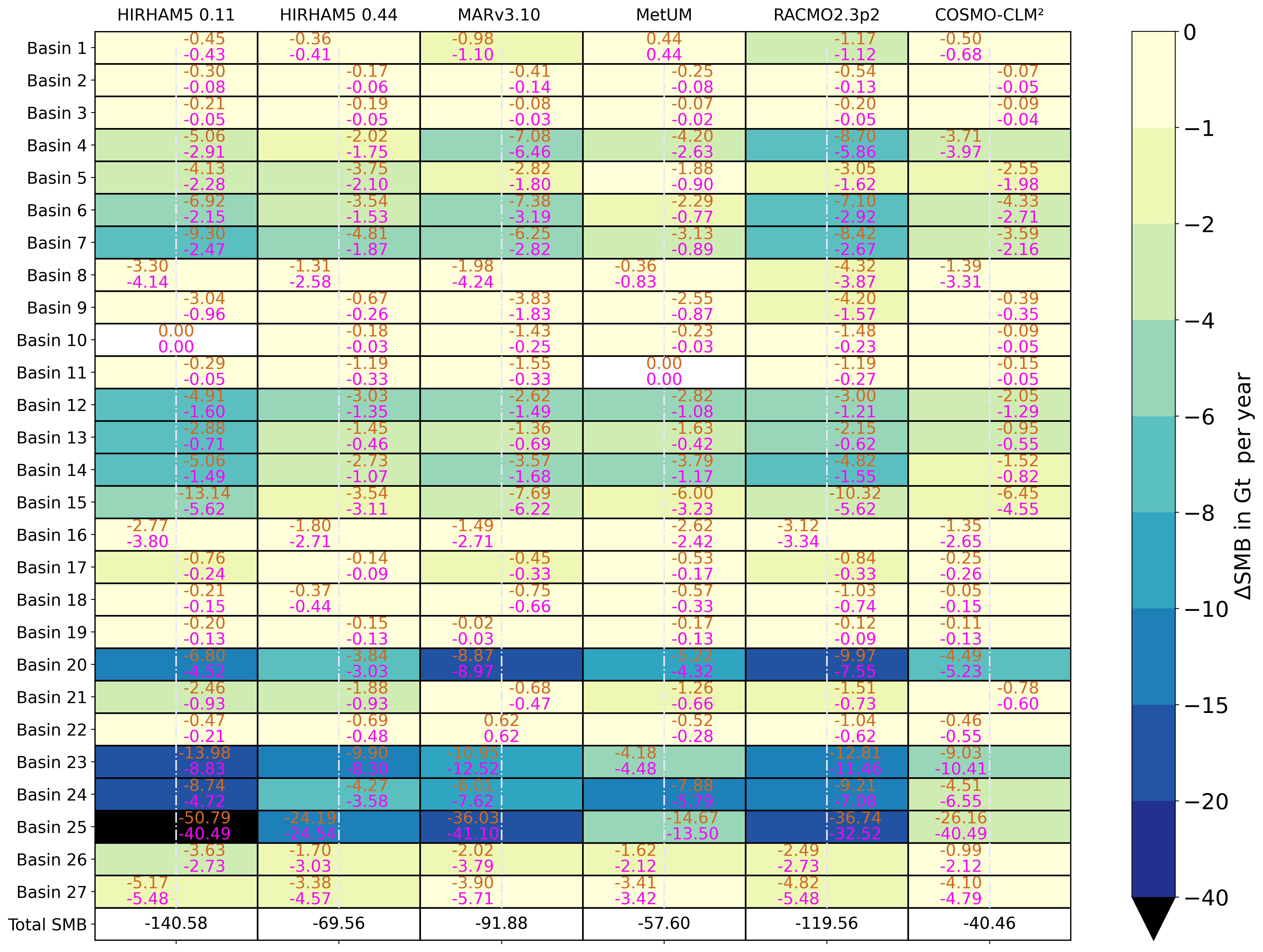
In order to investigate the regional and basin-scale variability, Table 2 shows values of Δarea%, ΔSMB% and ΔSMBGt yr-1 for each of the models and for each basin. ΔSMBGt yr-1 for basins 20, 23, 24 and 25 is the most sensitive to changes in the mask definition, up to 42.2 Gt yr−1. Of these four, two basins (20 and 23) are in West Antarctica and two on the windward side of the Antarctic Peninsula (24 and 25). Furthermore, the relative difference between Δarea% and ΔSMB% in the model–basin combinations shows large variability between the models and between the basins (Table 2). Summed over all the basins COSMO-CLM2 has the smallest relative difference between Δarea% and ΔSMB%. COSMO-CLM2 also has the smallest ΔSMBGt yr-1 integrated over the 27 basins, which shows that COSMO-CLM2 is the least affected by the change in ice mask (Table 1). Examination of Mottram et al. (2021) shows that COSMO-CLM2 is the driest model in the intercomparison and HIRHAM5 0.44∘ is the wettest, followed by HIRHAM5 0.11∘ and RACMO2.3p2. All six model simulations show differences of between 0 and −2 Gt yr−1 in ΔSMBGt yr-1 in basins 2 and 3, which have outlets to the Weddell Sea; basins 8, 9, 10 and 11 surrounding the Amery ice shelf; basins 16, 17, 18, 19 surrounding the Ross ice shelf; basin 22 with an outlet in the Amundsen Sea; and basin 27 on the lee side of the Antarctic Peninsula. Of these 12 basins, 8 of them are in East Antarctica.
Table 2Rows 1 to 27 are basins, and the columns are the RCMs. There are two numbers in each grid cell: the bottom number in magenta is the difference in area between the common mask and native masks (Δarea%) in each basin. The upper number in orange shows the difference in SMB between the common mask and native masks (ΔSMB%) in each basin. The grid cell colour shows the difference in SMB in Gt yr−1 (ΔSMBGt yr-1). All calculations are derived by subtracting the native mask from the common mask (Δ = common − native). The differences are shifted left if Δarea% is greater than ΔSMB% and right if ΔSMB% is greater than Δarea%. The bottom row is the summed ΔSMB values over 27 basins, for each model.
We find the differences between common and native ice mask areas to be small (<3 %), but they alter the SMB by up to 6 % over the ToAIS (140.6 Gt yr−1) when compared to the ensemble mean from Mottram et al. (2021). RACMO2.3p2, MARv3.10 and HIRHAM5 0.11∘ all have ΔSMBGt yr-1 values close to or larger than their given uncertainties for their respective SMB estimate. This means that the effect of using the common mask in estimating SMB is close to or greater than the standard deviation of annual mean SMB estimates derived from the interannual variability in modelled SMB. We consider the standard deviation to be a minimum estimate of uncertainty within each model with actual uncertainties likely to be considerably larger but difficult to estimate accurately (Lenaerts et al., 2019). Over the grounded AIS the common mask alters the SMB by up to 102 Gt yr−1; see Table 1. This difference in SMB is close in magnitude to the grounded AIS mass loss of 109±56 Gt yr−1 between 1992 and 2017 determined by the second Ice Sheet Mass Balance Inter-comparison Exercise (IMBIE2; Shepherd et al., 2018) and thereby essentially determines if the AIS is losing or gaining mass. This means that small changes in SMB can lead to a non-negligible change in the total mass budget of the AIS. The model mean of the grounded ΔSMBGt yr-1 is 54.2 Gt yr−1, which would make a sizeable change in the mass balance results (Table 1). Basin 25 has few or no ice shelves; thus it has one of the largest impacts for ΔSMBGt yr-1 for both the grounded basin (not shown) and when ice shelves are included.
Given the importance of the ice shelves to the dynamics of grounded ice, we argue that they are important to include in SMB models accurately. Furthermore, we speculate that there may be similar considerations when defining the grounded ice sheet for SMB assessments. This clearly shows the RCMs ice mask is key in integrated assessments of the Antarctic mass balance. These differences between area change and SMB change are the result of the area differences being located in the coastal regions, some of which are also high-relief regions, leading to effects on the SMB that are disproportionately high relative to the area.
In each grid cell between one and six native masks can have ice in them; this results in 63 combinations of model coverage, in addition to the common mask (not shown). These different area coverage combinations around the ice sheet are partly driven by differences in ice masks and partly by differences in resolution. However, we cannot identify any systematic or model-specific biases on a regional scale. The native ice masks vary around the coastline arbitrarily, which is partly due to the time when the ice mask was created and what data are used to create the native ice mask. For example, the HIRHAM5 and MetUM ice masks are created from data collected 3 decades ago, yet there have been multiple calving events since the data collection. The native ice masks from COSMO-CLM2 and MARv3.10 are created from data collected more recently and in a higher resolution. The higher resolution is also a benefit over the Antarctic Peninsula and in coastal areas where there is complex orography, where a higher resolution can also change the orographic precipitation.
The common mask is introduced during the post-processing stage after running the RCMs with their native masks. This has the disadvantage that model variables where the fluxes are linked to the orography, such as precipitation, can introduce a bias if the native mask is located differently in the domain compared to the common mask. The same orography bias can be true for winds and thus the sublimation rates as well. High precipitation rates are often strongly linked to the steep orography in coastal areas around Antarctica, especially in West Antarctica and on the windward side of the Antarctic Peninsula (basins 24 and 25), which is also where we see the largest differences in ΔSMBGt yr-1 in Table 2. Comparing the size of the common mask with the REMA mask over the Antarctic Peninsula shows that the common mask is smaller around most of the coastline (Fig. 1b).
The large differences in ΔSMBGt yr-1 and Δarea% found in this study suggest the need for more work to be done on a community basis to define a common mask, ideally before further RCM runs are conducted with the aim of contributing to any model intercomparison study. As the computational demands vary from model to model, we cannot expect the modelling groups to run on the same spatial grid resolution. Therefore, we suggest a three-stage effort be undertaken:
Step 1. Agree on a state-of-the-art DEM of the Antarctic continent, with a sufficiently high spatial resolution to be appropriate for even kilometre and sub-kilometre models (Orr et al., 2021). This could in our minds be REMA (Howat et al., 2019) at a 100 m grid resolution. This 100 m grid would form the basis for a community grid.
Step 2. Agree on a state-of-the-art delineation of surface types, such as bare rock, ice shelves or ice sheet, for the Antarctic continent, again with the highest possible resolution. Here, we see the grid-independent delineation of Antarctic glaciers as provided by the Randolph Glacier Inventory's shapefiles (RGI Consortium, 2017), combined with the shapefiles from the High resolution vector polygons of the Antarctic coastline data set (Gerrish et al., 2021) as a possibility. These two will then be combined to give the ice mask on the 100 m grid.
Step 3. Provide the community with a common tool for projecting the 100 m grid onto the RCM grid. We suggest that this tool will as a minimum give the variables to be used in further model intercomparisons – grid area (we suggest the Antarctic domain as defined in the Coordinated Regional Climate Downscaling Experiment (CORDEX)); surface elevation; surface types so one can distinguish between grounded ice, floating ice (glaciers/tongues) and rocks/mountain ridges; and ice-cover percentage. The ice-cover percentage will then provide the information needed to have the models contributing equally despite being run at different model resolutions, as the topography of the ice sheet is the same for all models. We imagine the tool consists of required data in a high resolution and a script that can create the grid file in the desired resolution, possibly in a netCDF format since most modelling groups are used to working in this format and it will be easy to handle. Ideally the ice mask would evolve over time as the continent changes; however, we feel it is important to first standardise the approach to creating and using ice masks. Thus, we suggest that it is noted in the mask file which data sets are used to create it and when the data sets were last updated.
We have quantified the importance of the choice of ice mask for the Antarctic domain by comparing six different ice masks from the RCM – COSMO-CLM2, HIRHAM5 (in two resolutions), MARv3.10, MetUM and RACMO2.3p2 – with the common mask defined by Mottram et al. (2021). We find differences of between 40.5 and 140.6 Gt yr−1 over the ToAIS and differences of between 20.1 and 102.4 yr−1 over the grounded AIS (Table 1), comparing the native mask to the common mask integrated over all the basins in Antarctica. Looking at individual basins, we find area differences from 0 % (HIRHAM5 0.11∘ basin 10 and MetUM basin 11) up to 40.49 % (HIRHAM5 0.11∘ basin 25) between the common and native masks (Table 2). Furthermore, area changes do not map to SMB change linearly (Table 2). The biggest differences are in basins 20, 23, 24 and 25, showing that areas with high SMB are most sensitive to mask differences (Table 2). As the native masks are created from different data sets, they do not all include the same ice shelves and ice tongues. We speculate that we introduce a shift in value by first defining the common mask after RCM simulations have been performed on their native masks. Most of the model variables in the SMB equation are sensitive to the orography and therefore sensitive to the representation of it when integrating over the common mask. The effort of defining a common mask should ideally be a community effort and should be done before conducting further model intercomparisons and contributing to joint assessments of mass balance such as the IMBIE assessment.
The common and native grid estimates of SMB over native and common masks are available at https://doi.org/10.11583/DTU.16438236.v1 (Hansen et al., 2021b).
NH, RM and SBS conceived the study and wrote the initial draft manuscript. Analysis of simulations was carried out by NH and SBS. Model simulation output and ice masks were provided by FB, CK, AO, JMvW and NS. All authors revised and contributed to the final manuscript.
The contact author has declared that neither they nor their co-authors have any competing interests.
Publisher's note: Copernicus Publications remains neutral with regard to jurisdictional claims in published maps and institutional affiliations.
Ruth Mottram and Fredrik Boberg acknowledge the support of the Danish state through the National Centre for Climate Research (NCKF). The COSMO-CLM2 team uses computational resources and services provided by the Flemish Supercomputer Center, funded by the FWO and the Flemish Government EWI department.
This project has received funding from the European Union's Horizon 2020 research and innovation programme (PROTECT contribution number 29 (grant no. 869304)). The COSMO-CLM2 integrations were supported by the Belgian Science Policy Office (BELSPO (grant no. 747 BR/143/A2/AEROCLOUD)) and the Research Foundation – Flanders (FWO (grant nos. 748 G0C2215N and GOF5318N; EOS ID 30454083)).
This paper was edited by Joseph MacGregor and reviewed by two anonymous referees.
Agosta, C., Amory, C., Kittel, C., Orsi, A., Favier, V., Gallée, H., van den Broeke, M. R., Lenaerts, J. T. M., van Wessem, J. M., van de Berg, W. J., and Fettweis, X.: Estimation of the Antarctic surface mass balance using the regional climate model MAR (1979–2015) and identification of dominant processes, The Cryosphere, 13, 281–296, https://doi.org/10.5194/tc-13-281-2019, 2019. a, b
Bamber, J. L., Gomez-Dans, J. L., and Griggs, J. A.: A new 1 km digital elevation model of the Antarctic derived from combined satellite radar and laser data – Part 1: Data and methods, The Cryosphere, 3, 101–111, https://doi.org/10.5194/tc-3-101-2009, 2009. a
Dupont, T. and Alley, R.: Assessment of the importance of ice-shelf buttressing to ice-sheet flow, Geophys. Res. Lett., 32, https://doi.org/10.1029/2004GL022024, 2005. a
Eidenshink, J. C. and Faudeen, J. L.: The 1 km AVHRR global land data set: first stages in implementation, Int. J. Remote Sens., 15, 3443–3462, https://doi.org/10.1080/01431169408954339, 1994. a
Fretwell, P., Pritchard, H. D., Vaughan, D. G., Bamber, J. L., Barrand, N. E., Bell, R., Bianchi, C., Bingham, R. G., Blankenship, D. D., Casassa, G., Catania, G., Callens, D., Conway, H., Cook, A. J., Corr, H. F. J., Damaske, D., Damm, V., Ferraccioli, F., Forsberg, R., Fujita, S., Gim, Y., Gogineni, P., Griggs, J. A., Hindmarsh, R. C. A., Holmlund, P., Holt, J. W., Jacobel, R. W., Jenkins, A., Jokat, W., Jordan, T., King, E. C., Kohler, J., Krabill, W., Riger-Kusk, M., Langley, K. A., Leitchenkov, G., Leuschen, C., Luyendyk, B. P., Matsuoka, K., Mouginot, J., Nitsche, F. O., Nogi, Y., Nost, O. A., Popov, S. V., Rignot, E., Rippin, D. M., Rivera, A., Roberts, J., Ross, N., Siegert, M. J., Smith, A. M., Steinhage, D., Studinger, M., Sun, B., Tinto, B. K., Welch, B. C., Wilson, D., Young, D. A., Xiangbin, C., and Zirizzotti, A.: Bedmap2: improved ice bed, surface and thickness datasets for Antarctica, The Cryosphere, 7, 375–393, https://doi.org/10.5194/tc-7-375-2013, 2013. a
Gerrish, L., Fretwell, P., and Cooper, P.: High resolution vector polygons of the Antarctic coastline (7.4) [Data set], UK Polar Data Centre, Natural Environment Research Council, UK Research and Innovation, https://doi.org/10.5285/cdeb448d-10de-4e6e-b56b-6a16f7c59095, 2021. a
Gudmundsson, G. H., Paolo, F. S., Adusumilli, S., and Fricker, H. A.: Instantaneous Antarctic ice sheet mass loss driven by thinning ice shelves, Geophys. Res. Lett., 46, 13903–13909, https://doi.org/10.1029/2019GL085027, 2019. a
Hansen, N., Langen, P. L., Boberg, F., Forsberg, R., Simonsen, S. B., Thejll, P., Vandecrux, B., and Mottram, R.: Downscaled surface mass balance in Antarctica: impacts of subsurface processes and large-scale atmospheric circulation, The Cryosphere, 15, 4315–4333, https://doi.org/10.5194/tc-15-4315-2021, 2021a. a, b
Hansen, N., Simonsen, S. B., Mottram, R., Orr, A., Boberg, F., Kittel, C., van Wessem, J. M., and Souverijns, N.: Brief communication: Impact of common ice mask in surface mass balance estimates over the Antarctic ice sheet, Technical University of Denmark [data set], https://doi.org/10.11583/DTU.16438236.v1, 2021b. a
Howat, I. M., Porter, C., Smith, B. E., Noh, M.-J., and Morin, P.: The Reference Elevation Model of Antarctica, The Cryosphere, 13, 665–674, https://doi.org/10.5194/tc-13-665-2019, 2019. a, b
Kittel, C., Amory, C., Agosta, C., Jourdain, N. C., Hofer, S., Delhasse, A., Doutreloup, S., Huot, P.-V., Lang, C., Fichefet, T., and Fettweis, X.: Diverging future surface mass balance between the Antarctic ice shelves and grounded ice sheet, The Cryosphere, 15, 1215–1236, https://doi.org/10.5194/tc-15-1215-2021, 2021. a
Lawrence, D. M., Fisher, R. A., Koven, C. D., Oleson, K. W., Swenson, S. C., Bonan, G., Collier, N., Ghimire, B., van Kampenhout, L., Kennedy, D., Kluzek, E., Lawrence, P. J., Li, F., Li, H., Lombardozzi, D., Riley, W. J., Sacks, W. J., Shi, M., Vertenstein, M., Wieder, W. R., Xu, C., Ali, A. A., Badger, A. M., Bisht, G., van den Broeke, M., Brunke, M. A., Burns, S. P., Buzan, J., Clark, M., Craig, A., Dahlin, K., Drewniak, B., Fisher, J. B., Flanner, M., Fox, A. M., Gentine, P., Hoffman, F., Keppel-Aleks, G., Knox, R., Kumar, S., Lenaerts, J., Leung, L. R., Lipscomb, W. H., Lu, Y., Pandey, A., Pelletier, J. D., Perket, J., Randerson, J. T., Ricciuto, D. M., Sanderson, B. M., Slater, A., Subin, Z. M., Tang, J., Thomas, R. Q., Val Martin, M., and Zeng, X.: The Community Land Model Version 5: Description of New Features, Benchmarking, and Impact of Forcing Uncertainty, J. Adv. Model. Earth Sy., 11, 4245–4287, https://doi.org/10.1029/2018MS001583, 2019. a
Lenaerts, J. T. M., Medley, B., van den Broeke, M. R., and Wouters, B.: Observing and Modeling Ice Sheet Surface Mass Balance, Rev. Geophys., 57, 376–420, https://doi.org/10.1029/2018RG000622, 2019. a, b, c
Loveland, T. R., Reed, B. C., Brown, J. F., Ohlen, D. O., Zhu, Z., Yang, L., and Merchant, J. W.: Development of a global land cover characteristics database and IGBP DISCover from 1 km AVHRR data, Int. J. Remote Sens., 21, 1303–1330, https://doi.org/10.1080/014311600210191, 2000. a
Mottram, R., Hansen, N., Kittel, C., van Wessem, J. M., Agosta, C., Amory, C., Boberg, F., van de Berg, W. J., Fettweis, X., Gossart, A., van Lipzig, N. P. M., van Meijgaard, E., Orr, A., Phillips, T., Webster, S., Simonsen, S. B., and Souverijns, N.: What is the surface mass balance of Antarctica? An intercomparison of regional climate model estimates, The Cryosphere, 15, 3751–3784, https://doi.org/10.5194/tc-15-3751-2021, 2021. a, b, c, d, e, f, g, h, i, j, k, l, m, n
Orr, A., Hosking, J. S., Hoffmann, L., Keeble, J., Dean, S. M., Roscoe, H. K., Abraham, N. L., Vosper, S., and Braesicke, P.: Inclusion of mountain-wave-induced cooling for the formation of PSCs over the Antarctic Peninsula in a chemistry–climate model, Atmos. Chem. Phys., 15, 1071–1086, https://doi.org/10.5194/acp-15-1071-2015, 2015. a
Orr, A., Kirchgaessner, A., King, J., Phillips, T., Gilbert, E., Elvidge, A., Weeks, M., Gadian, A., Kuipers Munneke, P., van den Broeke, M., Webster, S., and McGrath, D.: Comparison of kilometre and sub-kilometre scale simulations of a foehn wind event over the Larsen C Ice Shelf, Antarctic Peninsula using the Met Office Unified Model (MetUM), Q. J. Roy. Meteor. Soc., 147, 3472–3492, https://doi.org/10.1002/qj.4138, 2021. a
RGI Consortium: Randolph Glacier Inventory – A Dataset of Global Glacier Outlines: Version 6.0, Technical Report, Global Land Ice Measurements from Space, https://doi.org/10.7265/N5-RGI-60, 2017. a
Shepherd, A., Ivins, E., Rignot, E., Smith, B., Van Den Broeke, M., Velicogna, I., Whitehouse, P., Briggs, K., Joughin, I., Krinner, G., Nowicki, S., Payne, T., Scambos, T., Schlegel, N., Geruo, A., Agosta, C., Ahlstrøm, A., Babonis, G., Barletta, V., Blazquez, A., Bonin, J., Csatho, B., Cullather, R., Felikson, D., Fettweis, X., Forsberg, R., Gallee, H., Gardner, A., Gilbert, L., Groh, A., Gunter, B., Hanna, E., Harig, C., Helm, V., Horvath, A., Horwath, M., Khan, S., Kjeldsen, K. K., Konrad, H., Langen, P., Lecavalier, B., Loomis, B., Luthcke, S., McMillan, M., Melini, D., Mernild, S., Mohajerani, Y., Moore, P., Mouginot, J., Moyano, G., Muir, A., Nagler, T., Nield, G., Nilsson, J., Noel, B., Otosaka, I., Pattle, M. E., Peltier, W. R., Pie, N., Rietbroek, R., Rott, H., Sandberg-Sørensen, L., Sasgen, I., Save, H., Scheuchl, B., Schrama, E., Schröder, L., Seo, K. W., Simonsen, S., Slater, T., Spada, G., Sutterley, T., Talpe, M., Tarasov, L., Van De Berg, W. J., Van Der Wal, W., Van Wessem, M., Vishwakarma, B. D., Wiese, D., and Wouters, B.: Mass balance of the Antarctic Ice Sheet from 1992 to 2017, Nature, 558, 219–222, 2018. a
Souverijns, N., Gossart, A., Demuzere, M., Lenaerts, J., Medley, B., Gorodetskaya, I., Vanden Broucke, S., and van Lipzig, N.: A New Regional Climate Model for POLAR-CORDEX: Evaluation of a 30-Year Hindcast with COSMO-CLM2 Over Antarctica, J. Geophys. Res.-Atmos., 124, 1405–1427, 2019. a, b
van Wessem, J. M., van de Berg, W. J., Noël, B. P. Y., van Meijgaard, E., Amory, C., Birnbaum, G., Jakobs, C. L., Krüger, K., Lenaerts, J. T. M., Lhermitte, S., Ligtenberg, S. R. M., Medley, B., Reijmer, C. H., van Tricht, K., Trusel, L. D., van Ulft, L. H., Wouters, B., Wuite, J., and van den Broeke, M. R.: Modelling the climate and surface mass balance of polar ice sheets using RACMO2 – Part 2: Antarctica (1979–2016), The Cryosphere, 12, 1479–1498, https://doi.org/10.5194/tc-12-1479-2018, 2018. a, b
Webster, S., Uddstrom, M., Oliver, H., and Vosper, S.: A high-resolution modelling case study of a severe weather event over New Zealand, Atmos. Sci. Lett., 9, 119–128, https://doi.org/10.1002/asl.172, 2008. a
Zwally, H. J., Giovinetto, M. B., Beckley, M. A., and Saba, J. L.: Antarctic and Greenland Drainage Systems, GSFC Cryospheric Sciences Laboratory, 2012. a, b, c, d, e