The sensitivity of satellite microwave observations to liquid water in the Antarctic snowpack

Surface melting on the Antarctic Ice Sheet has been monitored by satellite microwave radiometry for over 40 years. Despite this long perspective, our understanding of the microwave emission from wet snow is still limited, preventing the full exploitation of these observations to study supraglacial hydrology. Using the Snow Microwave Radiative Transfer (SMRT) model, this study investigates the sensitivity of microwave brightness temperature to snow liquid water content at frequencies from 1.4 to 37 GHz. We first determine the snowpack properties for eight selected coastal sites by retrieving profiles of density, grain size and ice layers from microwave observations when the snowpack is dry during wintertime. Second, a series of brightness temperature simulations is run with added water. The results show that (i) a small quantity of liquid water (≈0.5 kg m⁻²) can be detected, but the actual quantity cannot be retrieved out of the full range of possible water quantities; (ii) the detection of a buried wet layer is possible up to a maximum depth of 1 to 6 m depending on the frequency (6–37 GHz) and on the snow properties (grain size, density) at each site; (iii) surface ponds and water-saturated areas may prevent melt detection, but the current coverage of these waterbodies in the large satellite field of view is presently too small in Antarctica to have noticeable effects; and (iv) at 1.4 GHz, while the simulations are less reliable, we found a weaker sensitivity to liquid water and the maximal depth of detection is relatively shallow (<10 m) compared to the typical radiation penetration depth in dry firn (≈1000 m) at this low frequency. These numerical results pave the way for the development of improved multi-frequency algorithms to detect melt intensity and the depth of liquid water below the surface in the Antarctic snowpack.

1 Introduction

Surface melting is frequent in summer in the coastal margins of the Antarctic continent and in particular on the low-elevation glacier termini, the ice shelves (Zwally and Fiegles, 1994). Monitoring melt is important not only as a climate indicator but also because of the potential influence of meltwater for the ice sheet's future fate. In the relatively cool conditions of the Antarctic, most of the meltwater usually refreezes in the firn, close to where it is produced. Runoff to the ocean is a small component of the meltwater cycle (Bell et al., 2017) and has a small contribution to sea level rise, unlike on the Greenland Ice Sheet (Agosta et al., 2019). However, through meltwater refreezing in place, an indirect and complex chain of processes leading to a potential significant mass loss has been evidenced (Scambos, 2004). Meltwater contributes to firn warming and air depletion which slowly weaken ice shelf structure over decades (Munneke et al., 2014; Lenaerts et al., 2016; Bell et al., 2018). In parallel, the small component of meltwater that does not refreeze in the firn may form supraglacial lakes (Banwell et al., 2014; Arthur et al., 2020) and surface streams (Dell et al., 2020). The drainage of these lakes enhances deep crevasse formation by hydrofracturing, providing one of the possible final triggers leading to shelf collapse (Banwell et al., 2013; Bell et al., 2018; Robel and Banwell, 2019; Leeson et al., 2020). Sea level rise follows from the resulting acceleration of the upstream land glaciers, against which the ice shelf previously acted as a buttressing force (Cook et al., 2005).

Surface melting occurrence is also a valuable climate indicator. The energy available for melt in Antarctica is relatively scarce, even in summer on the low-lying ice shelves, and is controlled by a variety of climatic variables (Jakobs et al., 2020). Warming of ice shelf surfaces by the air is a major driver (Torinesi et al., 2003a), but shortwave radiation and the intense downwelling longwave radiation during atmospheric rivers (Wille et al., 2019) are also important drivers. Locally, foehn effect has been shown to drive melt patterns on the Larsen C shelf at the foothills of the Graham Land mountain barrier (Luckman et al., 2014; King et al., 2017). On the Antarctic Peninsula, the occasional winter melt events are usually attributed to foehn winds (Munneke et al., 2018) and atmospheric rivers (Wille et al., 2019, 2022). At the continental scale, no long-term positive trends are apparent in the melt records over ice shelves (1979–2021) so far, despite local evidenced warming (Johnson et al., 2021). However change in the westerlies' strength blowing around the continent has been shown to be significantly correlated with melt occurrence (Picard et al., 2007; Johnson et al., 2021). The El Niño–Southern Oscillation also imprints a subtle signature on melt in the coasts of the Pacific sector (Johnson et al., 2021). For all these reasons, the ability to accurately monitor melt in Antarctica is important.

The detection of the state of surface melting using remote sensing has received a lot of attention since the inception of spaceborne microwave radiometry in 1970s (Ridley, 1993; Zwally and Fiegles, 1994; Abdalati and Steffen, 1997; Torinesi et al., 2003a; Colosio et al., 2021) and later using scatterometers and synthetic aperture radars (Kunz and Long, 2006; Johnson et al., 2020). The detection is in principle relatively easy because the apparition of liquid water in snow induces a sharp changes in the microwave signal. Most detection algorithms used in Antarctica monitor the microwave radiation at a single frequency and polarization and classify the surface as melting when the brightness temperature reaches a predetermined upper threshold. Other algorithms use a combination of channels (different frequencies and/or different polarizations) or more advanced detection techniques (Liu et al., 2006), but all are similar in essence.

Despite the abundance of work and the apparent simplicity of the detection, there are several unknowns that prevent optimal use of the satellite information: (1) the minimum amount of liquid water to enable the detection is not well known (Mote and Anderson, 1995; Tedesco et al., 2007), and this amount may vary across regions and years. Knowing this minimum amount is not so important when melt observations are used as a broad climate indicator (Picard et al., 2007; Johnson et al., 2021) but becomes critical at small spatial or temporal scales (Banwell et al., 2021) or for the evaluation of firn models which predict liquid water content (Kuipers Munneke et al., 2012). (2) When the wet snowpack is overlaid by a dry snow layer – e.g., due to snowfall, blowing snow, night refreezing or percolation of meltwater at depth – the microwave observations may still reveal the presence of underlying water because of the microwave penetration. For this reason, it is inappropriate to interpret the liquid water detected by microwave observations as “surface melting” strictly (Torinesi et al., 2003a). Nevertheless, it is not precisely known up to what depth water can be detected. This depth is likely to change during the melt season due to snow metamorphism (i.e., grain coarsening, densification, formation of ice layers). A better estimation of this depth is required, particularly in the context of multi-frequency sensor missions that could provide more advanced information on the fate of meltwater, percolation, refreezing and runoff in and on the snowpack (Leduc-Leballeur et al., 2020; Mousavi et al., 2021). (3) Most algorithms produce a surface melting binary indicator, but there is also a great interest in the quantification of meltwater volume and of the melt rate (Trusel et al., 2013) as predicted by surface energy budget and climate models (Kuipers Munneke et al., 2012; Fettweis et al., 2011). However, the possibility of retrieving such advanced information from microwave observations is debated, and limitations and possible accuracy need to be assessed. (4) When the surface becomes extremely wet (i.e., a saturated water layer, running water, surface ponding), the microwave brightness temperature decreases – because open water surfaces have a low emissivity (Comiso et al., 2003) – up to the point that melt detection may become impossible despite the surface being obviously wet. To our knowledge, existing products do not take this limitation into account. More specifically, the areal fraction of a pixel covered by supraglacial lakes, above which melt detection becomes impossible, remains to be quantified.

This study works to fill the four knowledge gaps outlined above by presenting a series of sensitivity analyses using microwave radiative transfer modeling. The focus is on the multi-frequency sensors (or combination of sensors) found in operational and in-preparation radiometry missions such as SMOS (Soil Moisture and Ocean Salinity; Kerr et al., 2010), SMAP (Soil Moisture Active Passive; Entekhabi et al., 2010), AMSR-E (Advanced Microwave Scanning Radiometer - Earth Observing System sensor), AMSR2, AMSR3 (Kasahara et al., 2020) and CIMR (Copernicus Imaging Microwave Radiometer; Kern et al., 2020). The overarching goal is to refine the interpretation of the datasets produced with the existing algorithms and to pave the way to new, more advanced, melt detection algorithms. This study is particularly aimed at users who need a better and more quantitative understanding of the various microwave melt products for detailed investigations and thorough firn model evaluations.

To conduct realistic simulations with wet snow, a pre-requisite is an accurate representation of the snowpack at the onset of the melt season. Given the lack of adequate in situ snow measurements in the Antarctic coastal marginal areas, our approach is to first retrieve the snowpack properties from the microwave observations. This is only possible when the snowpack is dry, before or after the melt season. Our method builds on ideas from Mote and Anderson (1995) and Brucker et al. (2010) but with a more advanced setup. It provides a simplified but realistic dry snowpack that can be then modified with added water in different proportions and depths to investigate the microwave sensitivity to liquid water.

The paper is structured as follows: Sect. 2 describes the microwave observations and the test sites. Section 3 outlines the radiative transfer model, the approach to retrieve the snowpack properties and the conducted simulations with added water in varying amount and depth. Section 4 presents the simulation results. Section 5 addresses the implication of the sensitivity analysis for the users of melt products and for algorithm developers.

2 Study sites and observations

Eight Antarctic coastal sites have been selected to investigate the sensitivity of microwave data to meltwater (Fig. 1 and Table 1). Five of them (Maudheimvida, Halvfarryggen, Larsen C, Larsen B and Roi Baudouin) are chosen due to the availability of detailed meteorological observations and melt estimates (Jakobs et al., 2020). Three other sites are located on major ice shelves and have a wide variety of conditions: Wilkins (high accumulation, presence of aquifer, Montgomery et al., 2020), Amery (low accumulation, presence of supraglacial lakes, Spergel et al., 2021) and Shackleton (high accumulation, Saunderson et al., 2022). All the sites are on ice shelves except Maudheimvida and Halvfarryggen. With firn and ice deeper than 100 m, the influence of the underlying substrate is only significant at the L band in dry conditions and is treated appropriately in our modeling setup.

Passive microwave observations acquired by the Advanced Microwave Scanning Radiometer 2 (AMSR2) on board Japan's Global Change Observation Mission – Water “SHIZUKU” (GCOM-W) satellite are used for the retrieval, general statistics and melt detection. Data at 6, 10, 19 and 37 GHz at vertical and horizontal polarizations are extracted from the National Snow and Ice Data Center (NSIDC) AMSR-E/AMSR2 Unified Level-3 Daily product, version 2 (Meier et al., 2018). The product has a resolution of 25 km at 6 and 10 GHz and 12.5 km at 19 and 37 GHz. The typical brightness temperature accuracy is ±1 K. Observations from the Soil Moisture Ocean Salinity (SMOS) from the European Space Agency (ESA), the Centre National d'Études Spatiales (CNES) and the Centro para el Desarrollo Tecnológico Industrial (CDTI) are also used to provide L-band data at 1.4 GHz (Kerr et al., 2001). We use the Level 3 product (Al Bitar et al., 2017) downloaded from the Centre Aval de Traitement des Données SMOS (https://www.catds.fr/, last access: 14 March 2022) and selected the nearest pixel of each site from the EASE-Grid 2 (Equal-Area Scalable Earth) in equatorial projection, which tends to be distorted in the polar regions (around 100 km in the meridian direction and 6 km in the zonal direction). The daily brightness temperature at 50–55^∘ viewing angle is extracted at both vertical and horizontal polarizations. The typical brightness temperature accuracy is ±2 K.

In this paper, the melt is detected both in the simulations and in the observations when the brightness temperature exceeds a threshold value calculated as the June to September mean brightness temperature (referred to as “dry brightness temperature” hereafter) +20 K. More elaborated algorithms exist (e.g., Mote and Anderson, 1995; Torinesi et al., 2003a; Johnson et al., 2020), but we choose the same fixed offset at all frequencies for the sake of simplicity and reproducibility of the results. The value of 20 K is lower than that used by Zwally and Fiegles (1994) but corresponds to a typical value of the adaptive algorithm by Torinesi et al. (2003a). The simulation results and analysis code are publicly available for further experiments with other algorithms (see the “Data availability” section).

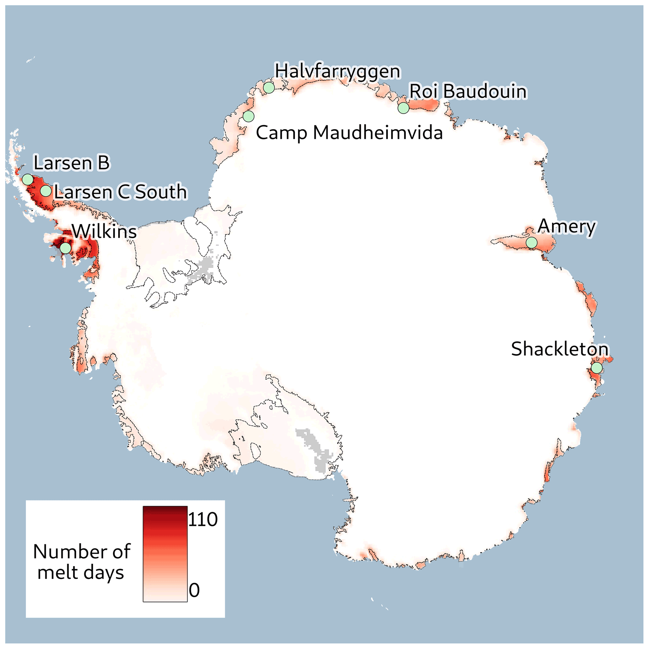
Figure 1 Map of Antarctica with the eight study sites. The annual mean number of melt days detected by the algorithm (Torinesi et al., 2003a) using AMSR2 19 GHz with horizontal polarization and ascending pass observations (2012–2022) is shown in red shading.

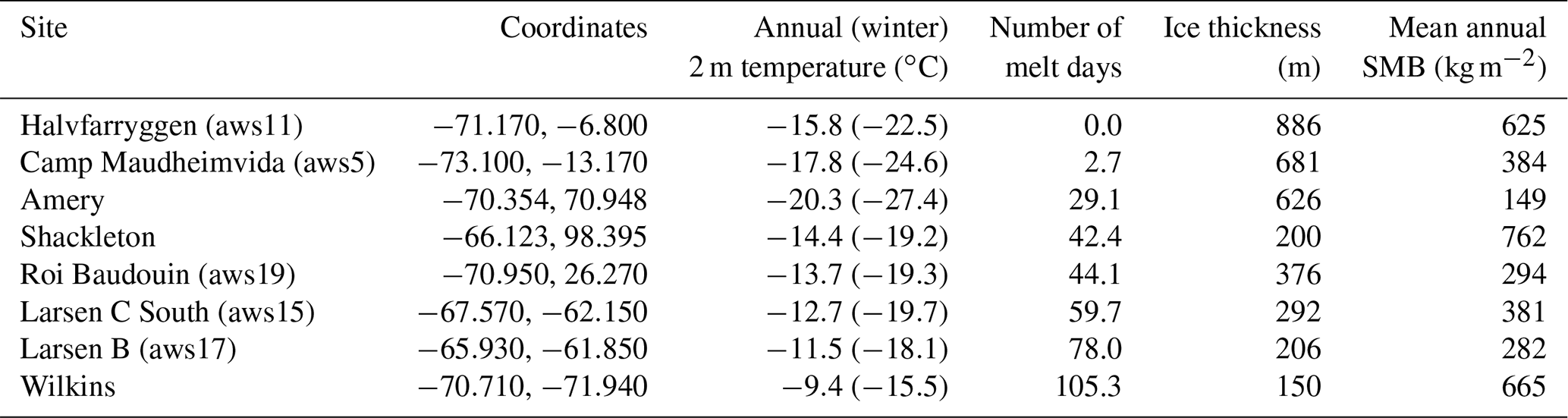
Table 1 Details of the eight sites selected to investigate the sensitivity of microwave data to meltwater. Automatic weather station (AWS) names are from Jakobs et al. (2020); temperatures are from the ERA5 reanalysis (Hersbach et al., 2020); melt days are from the AMSR2 19 GHz H-pol (horizontal polarization) channel (Torinesi et al., 2003a); ice thickness is from Bedmap2 (Fretwell et al., 2013); surface mass balance (SMB) is from RACMO (Regional Atmospheric Climate Model; Van Wessem et al., 2014).

3 Method

3.1 The Snow Microwave Radiative Transfer model

Brightness temperature simulations are run with the Snow Microwave Radiative Transfer (SMRT) model (Picard et al., 2018). This model is one-dimensional, and it represents the snowpack with horizontal layers. In each layer, the snow microstructure representation, temperature and liquid water content must be prescribed. Here, we selected the exponential microstructure representation which imposes to provide in addition the density and the correlation length for each layer (Sandells et al., 2021). Very similar results would be obtained with a different microstructure representation as long as the same microwave grain size is used, as demonstrated in Picard et al. (2022a).

Once the snowpack parameters are set, the model computes scattering in every layer using one of the theories available in SMRT (Picard et al., 2018). Here we selected the symmetrized strong contrast expansion, recently introduced in Torquato and Kim (2021), for general random porous media and applied to snow in Picard et al. (2022b). This theory has the advantage of treating the ice and air components of the snow microstructure in a symmetrical way so that the scattering function is continuous over the whole range of ice fractions (0–1). Before the use of this method, these functions were discontinuous when the ice components become preponderant with respect to air in the firn (i.e., around a density of $\mathrm{917}/\mathrm{2}=\mathrm{457}$ kg m⁻³). In a last step, SMRT solves the multi-layer radiative transfer equation using the discrete ordinate method (Picard et al., 2018). Atmospheric absorption and emission are neglected here due to the low frequencies and the relatively cold and dry Antarctic atmosphere. The output is the brightness temperature of the snowpack at two polarizations (vertical and horizontal) and at 55^∘ incidence angle for both AMSR2 and SMOS, close to the Brewster angle. Most simulations are run for a single point, but some are run at multiple points to account for the heterogeneity within large pixels. The resulting brightness temperature over such a pixel is the average of the results at all points.

3.2 Wet snow permittivity

The main effect of the liquid water in snow with respect to microwaves is to increase both the real and imaginary parts of the complex effective permittivity. Hence, estimating the effective permittivity of the water, ice and air mixture is an important step to investigate the sensitivity of microwaves to the water content and especially to determine the minimal detectable amount of water. However, no perfect permittivity formulation exists despite tremendous efforts in the 1970s and 1980s (Tiuri and Schultz, 1980; Sihvola et al., 1985; Hallikainen et al., 1986; Mätzler, 1987, and references therein).

In a nutshell, two main regimes of wetness must be distinguished (Colbeck, 1980) depending on the low or high volumetric water content. In the pendular regime, the volumetric water content is low (<3 %–7 % of the total snow volume) and the water appears as isolated inclusions in the pore space (i.e., between the ice grains), usually at the joints and in the necks, where the surface tension energy is minimal. A possible representation in this regime is to consider isolated water inclusions mixed in a dry snow background. In this case, the Maxwell Garnett (MG) mixing formula applies (Sihvola, 1999). However, a delicate choice remains for the shape of these inclusions that controls the depolarization factor in this formula (Colbeck, 1980; Mätzler, 1987).

In the funicular (>3 %–7 %) regime, water forms a continuous shell around the ice and the air pores become isolated (a non continuous phase). By assuming spherical ice grains coated by a thin water shell, the MG mixing formula applies if the water is the background and ice is the inclusions (Chopra and Reddy, 1986). This result is counterintuitive since the water is usually in the minority, but it can be understood by the fact that the electromagnetic waves mainly interact with the outer part of the grains, which is with the thin water shell. This model coincidentally has the advantage of describing saturated snow well, as water actually occupies the background, ice grains are isolated and air is virtually absent in this case. For testing, we also consider the MG mixture of water droplets in an ice background (called here the water pocket model). In both cases, to account for the air, the Polder and van Santen formula (Polder and van Santen, 1946) can be used to mix the air and one of these “wet ice” mixtures.

Countless other mixing strategies and empirical fits are possible, resulting in significantly different permittivity formulations. A number of them have been added in SMRT for this study. For a few of these formulations, Fig. 2 shows the real and imaginary parts of the permittivity as a function of the liquid water content ranging from zero (dry snow) up to the saturation point (no air) for the various sensitivity tests. All formulations agree on the fact that the permittivity (for both real and imaginary parts) increases with the water content due to the significantly higher water permittivity with respect to that of ice and air. However, differences between the formulations are large, for both the real and imaginary parts.

The formulations shown with circles in Fig. 2 are based on dielectric measurements of wet snow, while the formulations shown with solid lines are solely based on theoretically mixing ice, air and water with spherical inclusions. The formulation for the pendular regime by Colbeck (1980) is designed for small amounts. Likewise, the formulations by Wiesmann and Mätzler (1999) and by Hallikainen et al. (1986) (used here with the version updated by Ulaby and Long, 2015) respond quasi-linearly to the water content because they were fitted with experiments including small water contents only. Their validity for high water contents is unknown. MEMLS v3 (Microwave Emission Model of Layered Snowpacks; Mätzler and Wiesmann, 2007) extends the formulation by Wiesmann and Mätzler (1999) for high contents. A first group of formulations features similar behavior for small water contents; it comprises the Colbeck (1980) pendular, Wiesmann and Mätzler (1999), MEMLS v3, and the coated spheres. At the other end of the range, near the saturation point, the coated spheres, the two-step mixing (ice + water) + air and both Colbeck (1980) models converge towards similar values ($\approx \mathrm{14}+j\mathrm{16}$). The water pocket model is an outlier, which is expected given that melting snow is unlikely to be made of water inclusions in the ice crystals.

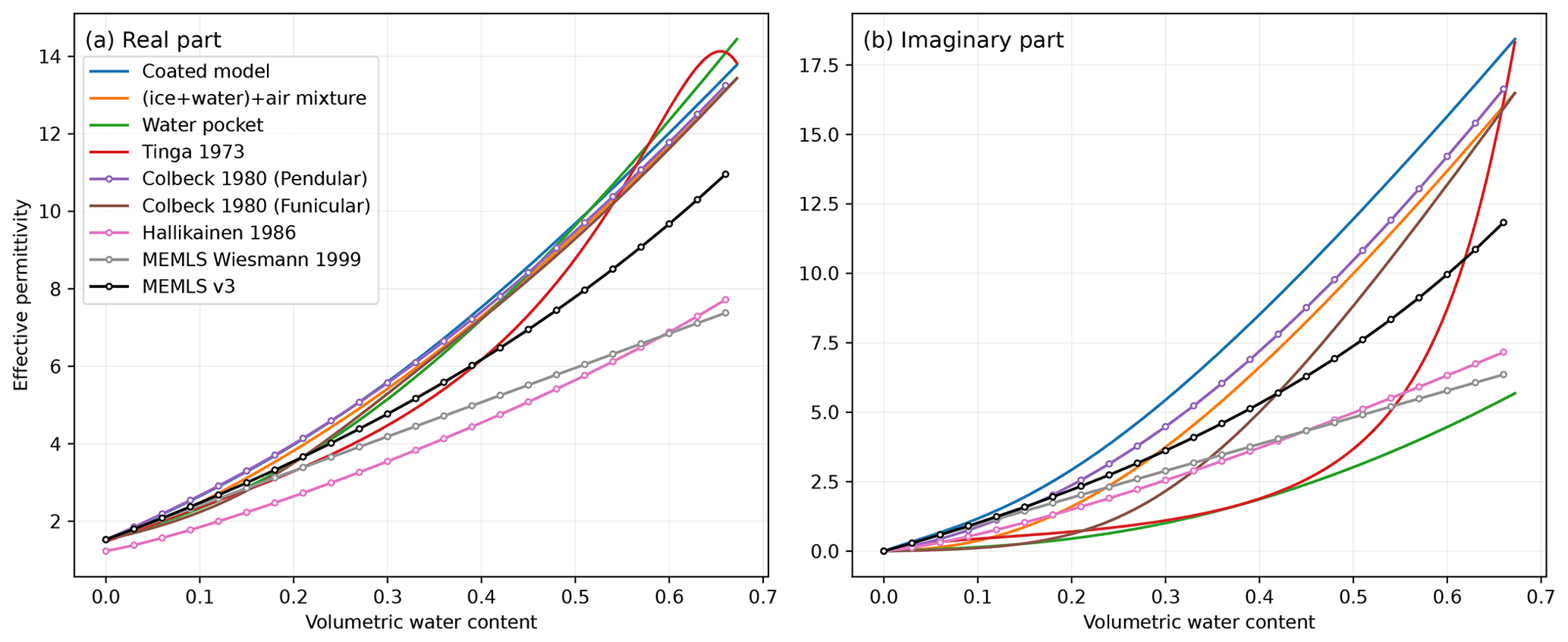
Figure 2 Real (a) and imaginary (b) parts of wet snow effective permittivity at 19 GHz, calculated with different formulations for increasing quantities of water filling the pore space of snow with an initial density of 300 kg m⁻³ up to the saturation point (i.e., until no air is left in the pores).

The fundamental reason for these large differences and lack of consensus is the extreme sensitivity of the effective permittivity to the depolarization ratio, which itself depends on the shape of the inclusions. Water inclusions in the pendular regime can be very elongated depending on the ice matrix. Until new permittivity and microstructure measurements are made, new developments are unlikely. A pragmatic choice between these formulations remains the only option.

In this study, we selected the MEMLS v3 formulation for the reference simulations because it is based on actual measurements and has an intermediate behavior. We also considered the formulation by Hallikainen et al. (1986) and show that it can not reproduce melting snow observations.

3.3 Retrieval of the dry snowpack properties

The effective snowpack properties are retrieved at all test sites independently, before and just after the melt season. We call these two periods “winter” (June–September) and “autumn” (April–May) for convenience. The retrieval is done by searching the optimal profiles of snow properties which lead to the best agreement between the microwave observations and SMRT output. We do not consider the temporal variations during the periods; only the averaged observations are used as input, and the output is a single “average” snowpack for each period. This retrieval approach builds upon previous work for the dry snowpack on the Antarctic Plateau (Brucker et al., 2010) and is also somewhat comparable to Mote and Anderson (1995) where the scattering of the snowpack is first optimized in winter to then better detect summer melt. Our approach differs mainly due to our consideration of a more complex snowpack. Specifically, here, the unknown snow properties include the correlation length, snow density and ice layer number density (given in number per meter). This triplet is able to drive the most dominant pattern of variations in brightness temperature. Density mainly controls the absorption and scattering; grain size controls the scattering; and the ice layer number controls the difference between the horizontal and vertical polarizations (H-pol and V-pol hereinafter). The terrain is assumed flat, and the surface roughness is neglected after preliminary tests performed with SMRT and the integral equation model (IEM) for rough surfaces (Brogioni et al., 2010) to determine the sensitivity of the brightness temperature in wet conditions to this snowpack characteristic. The profiles of the properties are assumed to be piecewise linear functions with four tie points at depths of 0, 3, 8 and 20 m, chosen to cover the range of e-folding depths at 6 GHz and higher frequencies. These tie points are the main unknowns of the optimization problem. At depths >30 m, the density is set constant to a typical value of 912 kg m⁻³ for deep firn (Burr et al., 2019) down to the base of the ice shelf (ice thicknesses are given in Table 1), where a saline water interface is added.

The temperature profile is prescribed for each season and site. It is approximated by superposing the seasonal temperature cycle penetrating down to d=2 m depth (Picard et al., 2009) and the overall steady gradient within the ice shelf resulting from the difference of surface and bottom temperature. The temperature profile is described by $T\left(z\right)=(T_{\mathrm{s}}-T_{\mathrm{a}})\exp (-z/d)+T_{\mathrm{a}}z/H+T_{\mathrm{w}}(H-z)/H$, where T_a and T_s are the mean annual and mean seasonal 2 m air temperatures, $T_{\mathrm{w}}=-\mathrm{2}$ ^∘C is the ice shelf bottom temperature, and H the shelf thickness. Air temperatures are from the ERA5 reanalysis (Hersbach et al., 2020).

To compute the optimal values and uncertainties at the tie points, we use Bayesian inference (Martin, 2022). The reason of this choice is first because we have only 8 observations (6, 10, 19 and 37 GHz at two polarizations, as L-band data are unused at this stage) for 12 unknowns (3 properties at 4 tie points). The minimization problem is under-determined, and the set of optimal properties is not unique. The second motivation is to account for the uncertainties in the model results with respect to the observations. We proceed as follows: each unknown is given a prior distribution, and the goal is to compute the joint posterior distribution of the unknown parameters of the model given the microwave observations. For the prior, we consider that little is known about the snowpack in these regions and choose uniform prior distributions with very wide ranges (also called uninformative priors) to avoid constraining the results with incorrect assumptions. The prior tie point densities are sampled in the ranges 200–700, 300–800, 400–910 and 400–910 kg m⁻³ respectively at the four depths; the grain sizes in the ranges 0–1.5, 0–2.5, 0–2.5 and 0–2.5 mm respectively at the four depths; and the ice layer number densities in the range 0–7 m⁻¹ at all depths. For the densities, we also add a constraint; the profiles with decreasing densities with depth are attributed a lower probability than those with increasing densities. The likelihood is set by assuming that the observations are normally distributed with zero mean (no bias between model and observation) and an unknown standard deviation σ to be determined by Bayesian inference at the same time as the 12 other unknowns. This standard deviation accounts for the observation uncertainties and representativeness error of the model (i.e., the simplification and the scale mismatch). After the priors and likelihood are set up, we compute the posterior with the differential evolution adaptive metropolis (DREAM) algorithm. This algorithm is an efficient Markov chain Monte Carlo (MCMC) method (ter Braak and Vrugt, 2008; Laloy and Vrugt, 2012; Shockley et al., 2017); 16 chains (recommended number between $d/\mathrm{2}$ and 2d, with d the number of unknowns) are run in parallel over 2000 iterations, and the first 50 % samples are discarded (“burn-in”). The output is an ensemble of 16 000 tie point sets following the posterior probability. However, the MCMC methods tend to produce auto-correlated samples, and in our case, the effective sample size as defined in Martin (2022) is estimated at ≈100. To assess the MCMC convergence, we calculated the potential scale reduction factor ($\widehat{R}$) (Gelman and Rubin, 1992) as provided by the ArviZ software (Kumar et al., 2019). Overall we obtain $\widehat{R}$ values lower than 1.2 for all parameters and all sites (in the burned-in ensemble) which is acceptable. For each site, the most probable posterior set (maximum a posteriori, MAP) is selected in the ensemble and used in the following sensitivity analyses. We also conduct some simulations with a large number of samples to investigate the impact of retrieval uncertainty on the sensitivity analysis.

In summary, after the optimization phase, we have, for each site and each season, many parameterized snowpacks to simulate the microwave observations, and one of them is the optimal. While it is tempting to analyze the retrieved properties of those snowpacks, it is important to recall that the problem is under-determined and the snowpack representation simplified. Many equifinal sets of parameters give similar brightness temperatures, despite potentially depicting quite different snowpacks from one another and from the real snowpack as well (Beven and Binley, 1992).

3.4 Wet snow simulations

To investigate the sensitivity of satellite microwave observations to liquid water, we ran simulations with the optimal dry snowpacks (for the winter season, unless otherwise stated) to which water was added in various quantities and at various depths. Water was always added by filling the air pores, which means that the ice mass (i.e., the dry snow density) is kept constant. In addition to generate a temperature profile representative of the summer season, we apply the same method as in winter except that T_s is set to 273 K.

We consider the following numerical experiments:

• Experiment 0 – dry snowpack;

• Experiment 1 – increasing water quantity in the superficial 10 cm thick layer;

• Experiment 2 – increasing water quantity in the superficial 1, 2, 5, 10 and 50 cm thick layer;

• Experiment 3 – increasing depth of a wet snow layer with a fixed volumetric water content and thickness (1.5 kg m⁻² and 10 cm);

• Experiment 4 – mixed pixel with a varying proportion of wet snowpack and supraglacial lakes.

4 Results

4.1 The dry snowpack – Experiment 0

Figure 3 shows the observed (triangles) and simulated (circles) winter brightness temperatures for each site at four AMSR2 frequencies and at the SMOS frequency in V-pol and H-pol. The sites are sorted by an increasing number of annual melt days.

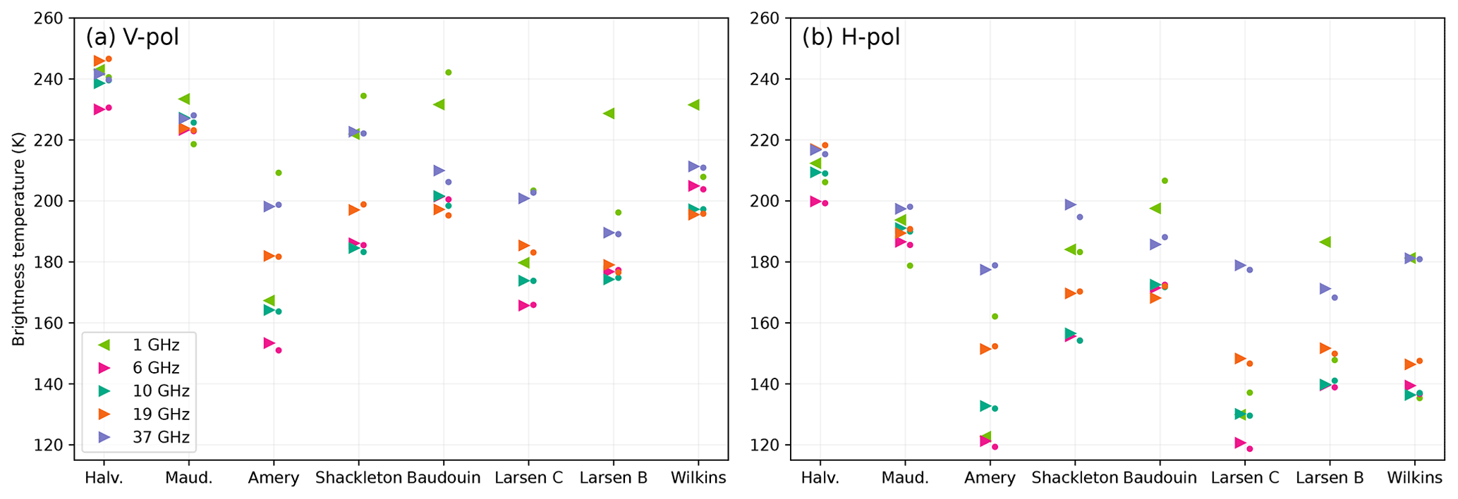
Figure 3 Observed (triangles) and modeled (dots) June–September brightness temperatures at vertical polarization (a) and horizontal polarization (b) for SMOS and AMSR2 frequencies. The sites are sorted by increasing number of melt days.

The brightness temperature varies by a much larger extent between the sites, 190–240 K at 37 GHz and 150–235 K at 6 GHz, than the variations in air temperature during wintertime (254–264 K), which indicates a dominant control by the emissivity that is itself determined by the snowpack structure. This indicates significantly different snowpacks from site to site.

The general trend is decreasing brightness temperatures with increasing numbers of melt days, which is particularly clear at the highest frequencies (19 and 37 GHz). Amery, despite a moderate number of melt days, stands out with the lowest brightness temperature among all sites. It may be related to its distinctively low SMB (Table 1). The H-pol follows in general the V-pol variations at the highest frequency, implying a fairly constant H $/$ V ratio over the sites (0.86–0.90). In contrast, the H-pol at 6 GHz presents a strong decreasing trend with the number of melt days, which translates into a decreasing H $/$ V ratio (from 0.9 to 0.7). Frequencies in between have an intermediate behavior. The 1.4 GHz frequency features large variations unrelated to the other frequencies. For instance, at H-pol, the brightness temperature is low and close to that at 6 GHz on Amery and Larsen C, whereas it is much higher and close to that of 37 GHz in the other sites. The reason for this is not clear.

In general, V-pol brightness temperature at the Brewster angle is mainly driven by volume scattering and snow temperature. The observed decreasing trend with the number of melting days (e.g., a 40 K decrease at 37 GHz) suggests that scattering is increasing with the number of melting days, probably because scattering is driven by the snow grain size and grain coarsening in the presence of water is much faster than in dry conditions (i.e., wet snow metamorphism; Colbeck, 1982). It must also be taken into account that fresh snowfalls counterbalance this coarsening by renewing snow at the surface with small grains. This may explain why high-accumulation areas (Shackleton and Wilkins) feature slightly higher brightness temperatures, despite a large number of melting days, and conversely why Amery has low brightness temperatures.

In general, the H-pol brightness temperature is more complex because it is in part controlled by snow scattering and snow temperature (exactly as V-pol), and in addition, it is sensitive to the surface density and the vertical density fluctuations in the snowpack (layering). The ice layers decrease the brightness temperature at H-pol due to the reflections on the high dielectric contrast between snow and ice in the upper part of the firn (Montpetit et al., 2013). The variations in V-pol and H-pol are correlated and of similar amplitude only if the ice layer effect is negligible. Here we find that at the highest frequency (37 GHz), the H-pol variations are close to that at V-pol. The reason is that the microwave e-folding depth is about 1 m (e.g., 1.3 m for Halvfarryggen and 0.75 m for Roi Baudouin) and only a limited number of layers are crossed by the upwelling radiation over such a small depth. In contrast, at the lowest frequencies, the e-folding depth is much larger (e.g., 11.5 m for Halvfarryggen and 5.2 m for Roi Baudouin at 6 GHz). The H-pol signal is lower than the V-pol signal due to the cumulative number of layers crossed by the upwelling radiation emitted in the snowpack at depth. The H-pol brightness temperatures and the H $/$ V ratios are therefore generally low at low frequencies.

The simulations with the optimal parameters for each site produce a good match with the observations at AMSR2 frequencies (dots in Fig. 3). The root mean square error (RMSE) is low, 1.3, 1.3, 1.7 and 2.0 K at 6, 10, 19 and 37 GHz respectively, accounting for both polarizations. These errors are comparable to the standard deviation σ estimated by the algorithm (all-site posterior mean of 2.5 K).

In contrast, the results for the L band (1.4 GHz) are very different. L-band simulations shown in Fig. 3 were obtained with a modified grain size profile because the simulations with the optimal parameters (not shown) present very large errors (33 K RMSE considering all sites and both polarizations). This may be partly explained by our choice to exclude the SMOS observations from the optimization. Nevertheless, the problem is more profound. To reproduce the SMOS observations, it is necessary to significantly increase scattering at 1.4 GHz (to simulate the low observed brightness temperature). This could be done by increasing the grain size (we found that an overall factor of ≈2.8 is necessary), but the collateral impact is degraded brightness temperatures at the higher frequencies. The snow grains are indeed small with respect to the wavelengths (Rayleigh scatterers), implying that their scattering spectral response is strongly increasing with the frequency (≈4th power of the frequency). Brucker et al. (2010) discuss a similar issue for 19 and 37 GHz on the East Antarctic Plateau. In other words, the relatively low brightness temperatures observed at the L band compared to those at higher frequencies are an indicator of the presence of large scatterers in the snowpack, i.e., probably ice nodules or pipes (Jezek et al., 2018). We chose not to add such scatterers in our snowpack representation because it would require an increased number of unknown parameters that would not be compensated by the additional observations provided by SMOS, making our estimation problem even more under-determined than it is. Instead, we devised a pragmatic approach. The grain size is multiplied by 2.8, for all the sites when only simulating the L-band brightness temperature (value obtained by successive tests), which leads to a reduced, but still relatively high, RMSE of 25 K. These results are shown in Fig. 3. We hypothesize that this approach works for the purpose of this study based on the fact that absorption becomes the dominant process over scattering when water is added. However, in general, the L-band results must be taken with caution. For this reason, these results are addressed in a dedicated section (Sect. 4.6) after the AMSR2 frequency results.

The mean retrieved parameters for all the sites are shown in Fig. 4. Some general observations can be made despite the risk of compensation between parameters (equifinality). It is also worth noting that the properties at 20 m are not always constrained by the observations, as for instance when the e-folding depth is only 5.2 m at Roi Baudouin at 6 GHz, the lowest frequency used in the optimization. In this case, the method returns a virtually random value for this depth. Nevertheless, we observed that the grains are systematically smaller near the surface and generally increase in size with depth, which is a consequence of the observed brightness temperature dependence on the frequency as explained in Brucker et al. (2010). This vertical distribution is expected because fresh, small-grained, snow is present in winter, overlying the wet-metamorphosed, coarse-grained, snow from the previous summer at depth. The sites with the high brightness temperatures (Halvfarryggen and Maudheimvida) have distinctly smaller grains at 3 m depth, which is consistent with the lack of melt at those locations. The density increases with depth. The ice layer number density at the top of the snowpack is around 1 m⁻¹ and slightly increases for sites with greater number of melt days. At a depth of 20 m, this number is higher and fairly constant around 4 m⁻¹ except at Wilkins. This increase in ice layer number density with depth can also be explained with an upper winter-snow layer with little stratification and a deeper snowpack containing ice layers that have been buried over time.

Figure 4 Grain size (i.e., correlation length), density and ice layer number density (i.e., number of layers per meter) at depths 0, 3, 8 and 20 m for each site in winter. Each triangle is the average over the 1000 best parameter sets. Note that for Halvfarryggen grain size, the two triangles for 0 and 3 m depth overlap, and the same applies at 3 and 8 m in Wilkins.

The results for the autumn snowpack (results not shown) highlights a decrease in brightness temperature at 37 GHz compared to the winter results, associated with a coarsening of the grains during the melt season (0.044 to 0.075 mm) and a slightly higher number of layers (1.3 to 1.5 mm) near the surface.

4.2 Variations with the water content in the surface layer – Experiment 1

4.2.1 The two microwave emission regimes illustrated at one site

An increasing amount of water is added in the top 10 cm layer of the dry snowpack for Roi Baudouin, an intermediate site in terms of melt and brightness temperature. The explored range is 0–20 kg m⁻², which corresponds to 0 %–20% in volume in the wet layer and about 0–50% in mass (the surface density of the best parameter set is 220 kg m⁻³). Figure 5 shows the results.

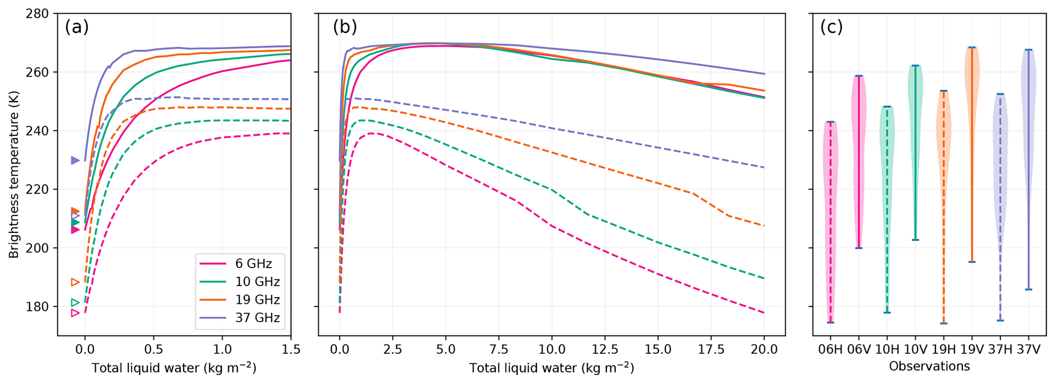
Figure 5 Brightness temperatures at Roi Baudouin as a function of the total liquid water content in the top 10 cm of the snowpack for four frequencies and at V-pol (solid curves) and H-pol (dashed curves) (a, zoomed in; b, full range). The simulated dry brightness temperatures are marked by the triangles. The seasonal air temperature is set to 273 K, which explains why the dry brightness temperatures are higher than in Fig. 3 where the winter seasonal temperature was used. Distribution of observed satellite brightness temperatures only for the days when the surface is melting (based on the melt rates computed from in situ measurements by Jakobs et al., 2020) (c).

The microwave signal is affected by the presence of liquid water in the snowpack according to two different microwave emission regimes. In the first regime, the sudden apparition of water at the surface of the ice crystal sharply increases the snow absorption because the imaginary part of the water permittivity is extremely high compared to that of ice (0.0017 at 19 GHz, Mätzler et al., 2006) (Fig. 2). As a result, the brightness temperature increases because the snowpack becomes a near black body. At V-pol, the brightness temperature reaches 271 K, which is very close to the perfect back body (273 K). This is a consequence of the observing configuration close to the Brewster angle; the vertically polarized emitted radiation is transmitted through the surface without any loss. In reality, such high brightness temperatures are rare; for example they can be found only 347 times in the full daily AMSR2 19 GHz records gridded at 12.5 km over nine summers (2012–2021). For comparison, melt is detected 2.5×10⁶ times on this same grid and for this same period. In contrast, the H-pol brightness temperature only reaches 240–250 K depending on the frequency because the surface reflects part of the snowpack emission back down. Despite this lower maximum, the amplitude of the increase is larger at H-pol than at V-pol (≈60 K versus 55 K), which is also the case in the observations (Fig. 5c) and is the reason why most single-channel detection algorithms use the H-pol.

Another important piece of information for the user of melt products is the water content threshold from which melt can be detected by the microwave sensor. This information is crucial for the validation of firn models for instance. We find that very small amounts of water of 0.11, 0.07, 0.05 and 0.06 kg m⁻² can be detected (assuming a +20 K H-pol increase) at 6, 10, 19 and 37 GHz respectively (values for the Roi Baudouin site). The sensitivity is slightly higher at 19 and 37 GHz because of the short wavelengths. These values are similar to those reported in previous work (Tedesco and Kim, 2006) using the coated permittivity model (the strongest absorption) and using MEMLS (Fig. 1 in Tedesco et al., 2007).

When the amount of water further increases, the brightness temperature reaches a maximum and then slowly decreases (Fig. 5b). In this second regime, the absorption is still very strong, but the effect of the high real part of the water permittivity becomes significant (Fig. 2). Note that the small slope changes (e.g., around 17.5 kg m⁻² at 19 GHz) is a numerical artifact due to this increasing strong permittivity and how SMRT deals with the refraction in the DORT method (discrete ordinate and eigenvalue; details in Picard et al., 2018). The wet surface becomes more and more reflective at H-pol (0.02 at 0 % and 0.27 at 20 % at 19 GHz), reducing the brightness temperature (Naderpour et al., 2017; Leduc-Leballeur et al., 2020). Then, the Brewster angle increases (from 49^∘ at 0 % to 63^∘ at 20 %) so that the V-pol brightness temperature at 55^∘ starts decreasing as well, though in a lesser proportion than at H-pol. The same behavior is observed on wet soils and is at the basis of soil moisture retrieval algorithms for SMOS (Kerr et al., 2001). In principle, snow wetness could be retrieved in this regime using H-pol brightness temperature or the H $/$ V ratio, as investigated by Naderpour and Schwank (2018).

The transition between the first, “absorption” regime and the second, “reflective” regime takes place around 0.75 and 1.75 kg m⁻² at 37 and 6 GHz respectively. Shi and Dozier (1995) reported a slightly higher value of 3 kg m⁻² for radar at the C band (5.6 GHz). Using a different formulation of the wet snow permittivity would change these values. For instance the coated sphere model (results not shown) has a higher imaginary part of the permittivity, which leads to even more rapid increases in the first regime and a reduced decreasing rate in the second regime because the absorption dominates even more than the scattering and reflection mechanisms.

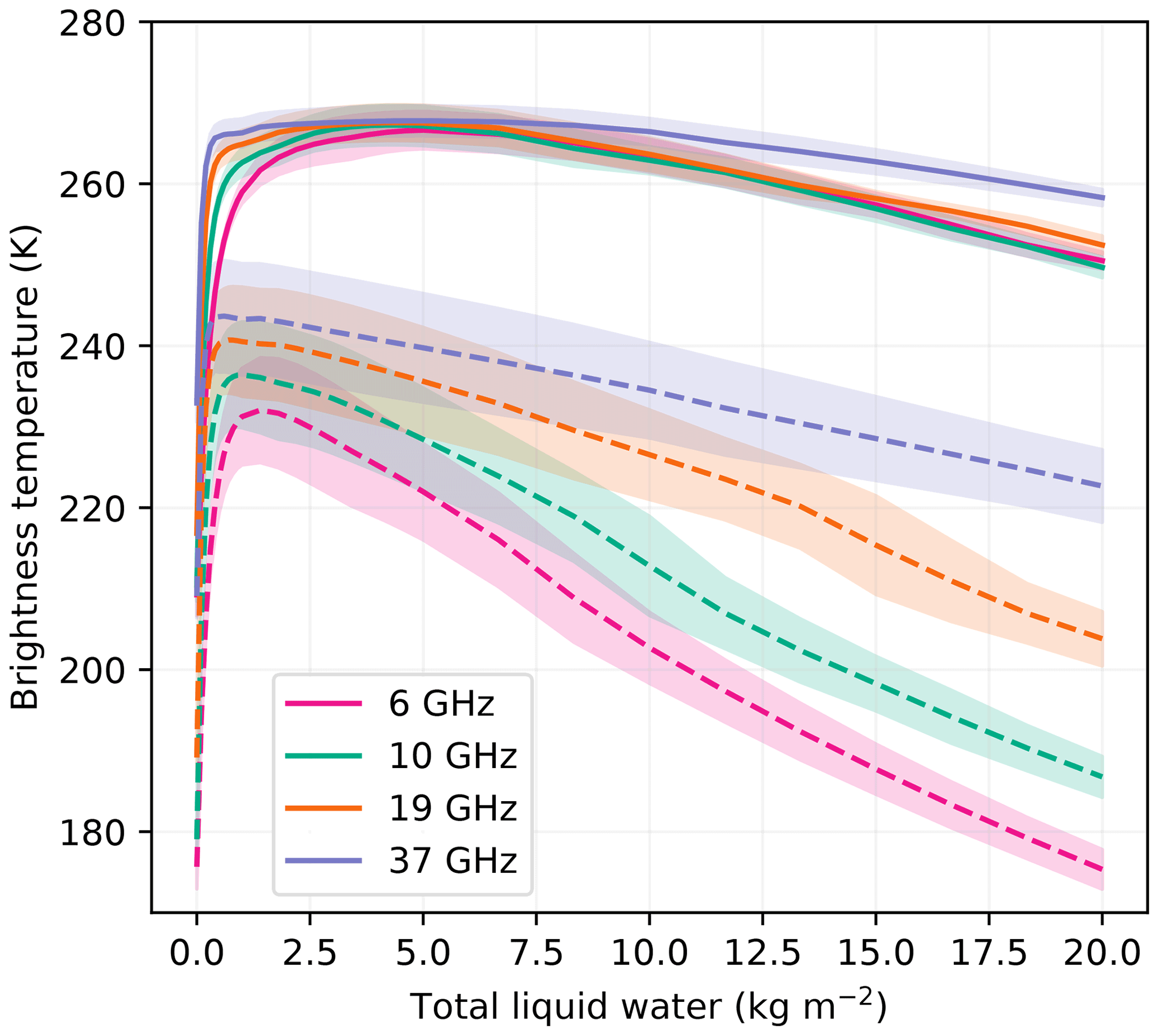
Figure 6 Brightness temperatures at Roi Baudouin obtained with the 1000 best (i.e., most probable) snowpacks as a function of the total liquid water content for four frequencies at V-pol (solid curves) and H-pol (dashed curves). The lines show the mean brightness temperature of the ensemble, and the shade areas materialize ±1 standard deviation around the mean.

Figure 6 shows the same sensitivity analysis for a large ensemble of most probable snowpacks provided by the Bayesian inference at Roi Baudouin. It highlights the impact of the uncertainties in the retrieved parameters on the brightness temperature when water is added. In the absorption regime, the impact is relatively small, and the threshold of detection and the transition limit to the reflective regime are stable across the simulations. Conversely in the reflective regime, the variability is large, especially at H-pol. By conducting additional simulations where all the snowpacks were set with a fixed density value at the surface (i.e., in the uppermost 10 cm layer only), we found a much weaker variability (results not shown). We conclude that the uncertainty in the surface density is the main cause of H-pol variability. This suggests that retrieving snow moisture could be improved by retrieving the surface density beforehand, a conclusion in line with the findings of Naderpour and Schwank (2018).

4.2.2 Intra-pixel variability

Because of the coarse resolution of the microwave radiometers (≈25 km), it is likely that the presence and quantity of liquid water in the snowpack is variable within a given pixel. Combined with the highly non-linear response shown in Fig. 5, this variability is able to affect the sensitivity analyzed in the previous section. To simulate such an heterogeneous pixel, we assume that the liquid water content follows a normal distribution, with negative values set to 0 kg m⁻² (dry snow), and compute the brightness temperature for 10 000 liquid water values sampled from this distribution. The resulting brightness temperature over such an heterogeneous pixel is the average of all these brightness temperatures. Figure 7 shows the resulting brightness temperature at 19 GHz as a function of the mean liquid water content in the heterogeneous pixel. The different curves correspond to different standard deviations of the normal distribution of total liquid water content (σ_TWC) before removing the negative values. The results clearly show a change of sensitivity. The rate at which the brightness temperature increases when the snowpack becomes wet becomes smaller and smaller as the heterogeneity increases, an expected outcome of the concavity of non-linear response shown in Fig. 5. The water content threshold from which melt can be detected is about 0.9 kg m⁻² for a 2 kg m⁻² standard deviation, a 10-fold increase compared to 0.08 kg m⁻² when the pixel is assumed homogeneous.

However, little is known about the distribution of surface melt rate and of the liquid water content over a 25 km pixel in reality. It is difficult to conclude whether σ_TWC≈2 kg m⁻² is a realistic value or not. The sources of liquid water content variability include the surface roughness, the large-scale terrain topography, the wind and cloudiness, dust deposition, snow density, snow grain size, etc. Future research should investigate the distribution of melt in more detail. Meanwhile, this result demonstrates that the uncertainty in the liquid water content heterogeneity is a major contributor to the uncertainty associated with relating brightness temperature values to liquid water content. Indeed, for a given observed brightness temperature value, many different mean liquid water contents are possible, reducing the possibility of retrieving accurate values of liquid water content from microwave radiometry.

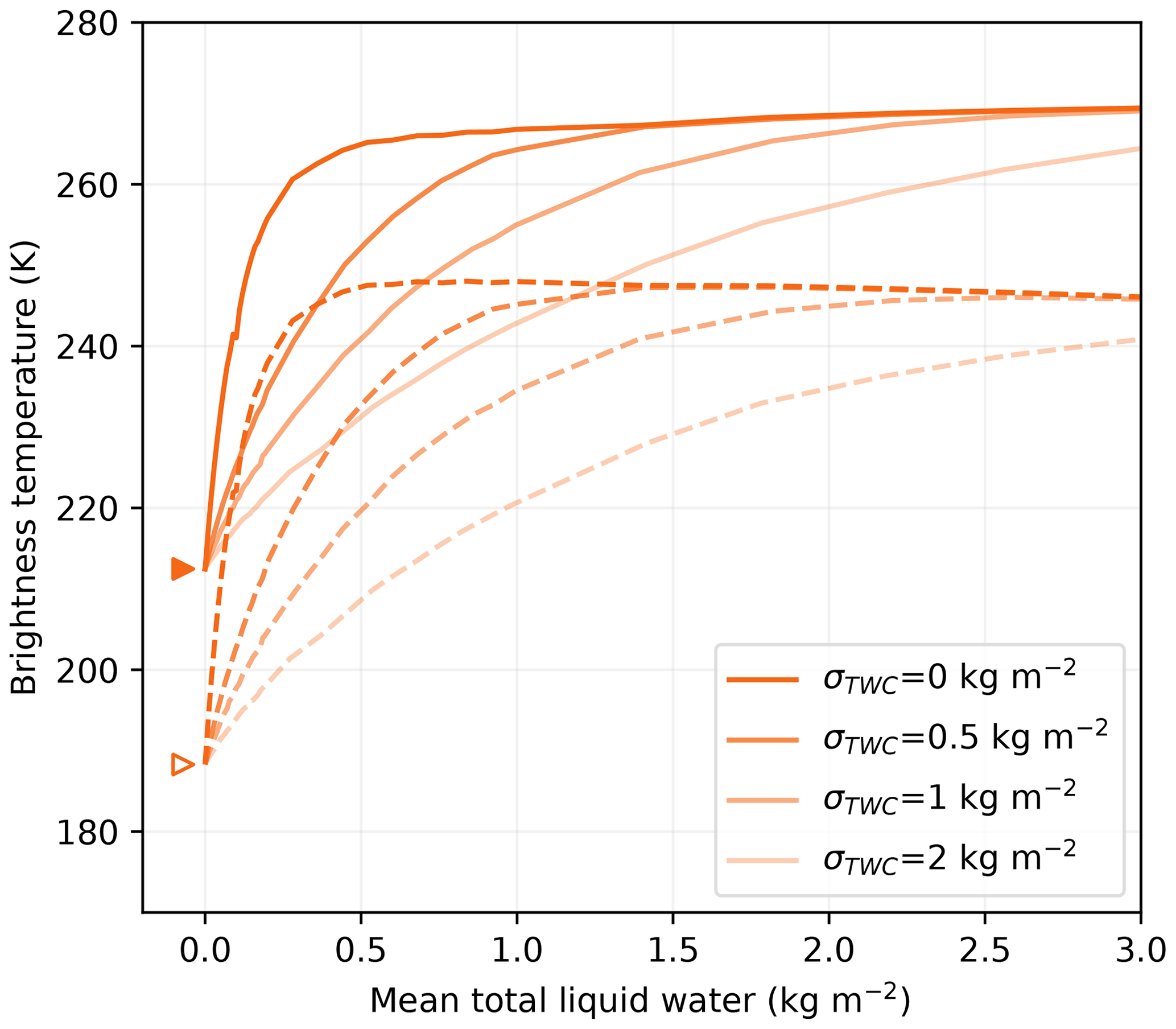
Figure 7 Brightness temperatures as a function of the total liquid water content at 19 GHz at V-pol (solid curves) and H-pol (dashed curves) at Roi Baudouin when the liquid water content is heterogeneous. σ_TWC is the standard deviation of the normal distribution used to generate local total liquid water content (negative values set to 0).

4.2.3 Inter-site variations

Figure 8 shows the brightness temperatures as a function of the total liquid water content (for smaller amounts than in the previous figures) for a homogeneous pixel for the best snowpack at every site at 19 and 6 GHz. The main characteristics observed at Roi Baudouin (two regimes, threshold, sensitivity, etc.) in Sect. 4.2.1 appear here to be general. The variability of the dry brightness temperature is large as already mentioned in Sect. 4.1, and it may impact the detection sensitivity and quality. This result is well known, and all detection algorithms use adaptive techniques to cope with this variability. For instance, Zwally and Fiegles (1994) take the detection threshold to equal the averaged H-pol winter brightness temperature over 9 years plus 30 K. Torinesi et al. (2003a) take a different threshold for each year equal to the averaged H-pol winter brightness temperature plus 3 times the standard deviation H-pol winter brightness temperature. However, a potential negative consequence of such an adaptivity is a variable sensitivity to liquid water content from site to site and year to year. Our simulations indicate that the detection limit is fairly constant between 0.03 and 0.04 kg m⁻² at 19 GHz (with the simple threshold of 20 K), except for the much higher value of 0.11 kg m⁻² for Maudheimvida and no value for Halvfarryggen, which has dry brightness temperatures too high to be detected. These latter sites with the highest winter brightness temperatures – where less melt occurred in the previous years – are also those sites with the lower sensitivity and also possibly a higher false-positive rate if the threshold is reduced below 20 K, in line with Tedesco (2009). This variability in the sensitivity motivated the development of a more advanced algorithm (Tedesco, 2009) where a radiative transfer model (MEMLS) estimates the brightness temperature threshold for a user-defined fixed water content depending on the snowpack characteristics.

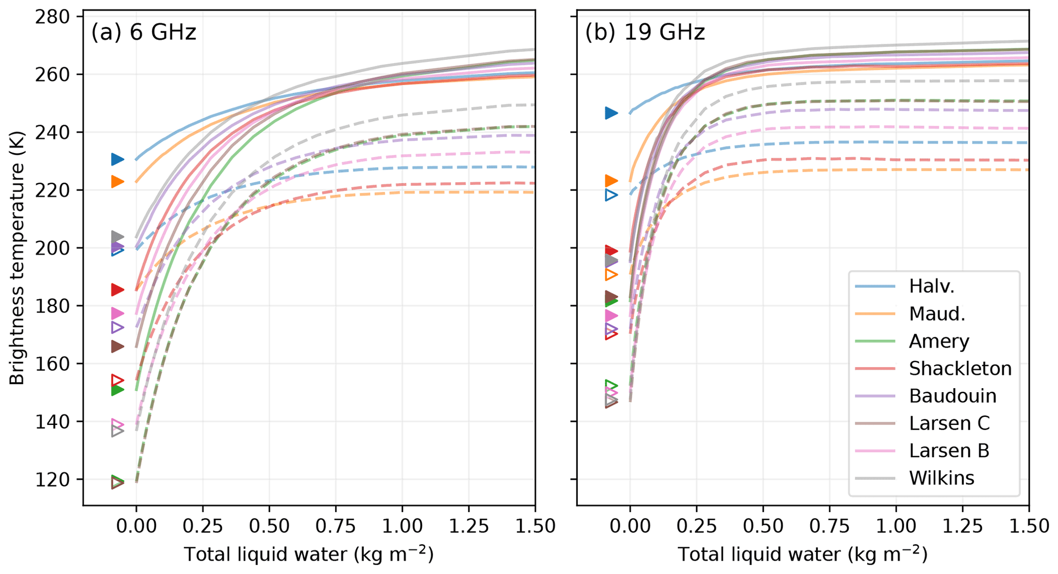
Figure 8 Brightness temperatures as a function of the liquid water content for all sites at V-pol (solid curves) and H-pol (dashed curves) at 6 GHz (a) and 19 GHz (b). The values of the dry brightness temperatures are marked by the triangles.

4.2.4 Impact of the permittivity formulation

The results presented in the previous sections rely on the selected permittivity formulation (MEMLS v3). To illustrate the importance of the formulation, we run simulations with the H86 formulation (Hallikainen et al., 1986; Ulaby and Long, 2015), which has a relatively extreme behavior compared to the selected formulation. The results in Fig. 9 depict a very different behavior of brightness temperature for small amounts of water. A marked minimum in brightness temperature is observed around 0.5 kg m⁻² at all frequencies and polarizations. This minimum is the signature of a “scattering regime”. Indeed the H86 formulation features a particularly low imaginary part, while the real part is not different from that of the other formulations. When the snowpack is transitioning from dry to wet, the scattering is enhanced by the rapidly increasing real part (i.e., snow grains become more reflective), while the absorption remains weak due to the low imaginary part. The consequence is a decreasing brightness temperature with increasing water content until the absorption starts increasing significantly, offsetting the scattering effect. The “scattering” regime dominates up to about 2.5 kg m⁻² when the brightness temperature recovers to the winter value and then further increases in the absorption regime as found with the MEMLS v3 permittivity formulation. To assess the relevance of H86 formulation, we explored a large number of time series of AMSR2 brightness temperatures around the Antarctic and never noticed such a decrease in brightness temperature caused by weak melt events. We therefore conclude that the imaginary part of H86 formulation is certainly inadequate to model wet snow.

Figure 9 Brightness temperatures at Roi Baudouin at V-pol (solid curves) and H-pol (dashed curves) computed with the permittivity formulation from Hallikainen et al. (1986) featuring a low imaginary part as a function of the total liquid water content (a, zoomed in; b, full range). The dry brightness temperatures are marked by the triangles.

4.3 Variations with the thickness of the wet snow layer – Experiment 2

The previous results were obtained with a fixed wet snow layer of 10 cm. Figure 10 reports a few results for different thicknesses of wet snow h_w (for Roi Baudouin and at 6 and 19 GHz only) considering two predictor variables (i.e., the variable on the x axis): the total liquid water content TWC (in kg m⁻²) or the volumetric liquid water content θ_i (a fraction, no unit, usually expressed in percent). These variables are related by TWC=θ_iρ_waterh_w, where ρ_water is the water density. We find that varying the thickness of the wet snow layer has little influence on the results if the total amount of liquid water is fixed (Fig. 10a), and in contrast, very large variations are observed if the volumetric liquid water content is fixed (Fig. 10b). This result is expected given that the brightness temperature is mainly driven by the absorption of the upwelling radiation through the wet snow layer and that this absorption is quasi proportional to the total mass of water, at least for small amounts of water (i.e., the imaginary part of the effective permittivity is linear for small amounts; see Fig. 2). It means that the results in the previous section generalize well if the layer thickness differs from 10 cm as long as the total liquid water content is used on the x axis. Despite this, many authors usually report results in terms of volumetric liquid water content (e.g., Tedesco and Kim, 2006; Naderpour and Schwank, 2018) because it is a measurable quantity and it naturally appears in metamorphism models. However, in this case, our results also show that it is crucial to clearly report the thickness of the wet layer.

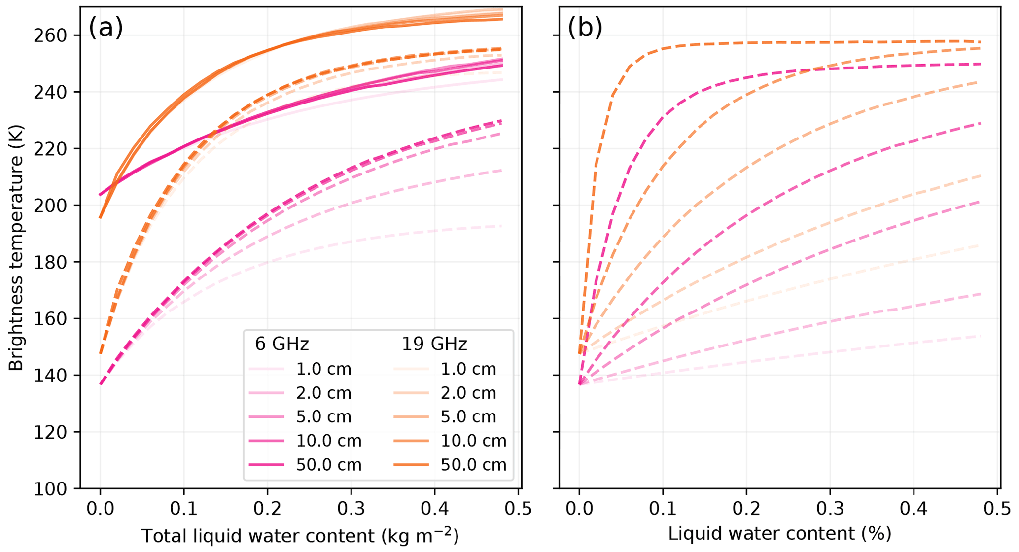
Figure 10 Brightness temperature as a function of the total liquid water content (a) and the volumetric liquid water content (b) for various wet snow layer thickness, for Roi Baudouin at 6 GHz (pink) and 19 GHz (orange), at V-pol (solid curves) and H-pol (dashed curves). V-pol is not on panel (b) for the sake of readability.

The case of thin wet snow layers (i.e., 1 and 2 cm) is particular. Figure 10a depicts a smaller increase in brightness temperature (especially at H-pol and 6 GHz) for the thinnest layers, compared to the thicker layers. We explain this specific finding by the high volumetric liquid water content in the thin surface layer, which leads to a high permittivity constant, a high reflectivity and in turn a low emissivity.

In conclusion, plotting brightness temperature variations as a function of the total liquid water content (kg m⁻²) allows for a better generalization of our results for other thicknesses than if the volumetric liquid water content was used. For this reason, we generally present our results in terms of total liquid water content.

4.4 Influence of the depth of the wet snow layer – Experiment 3

Because of refreezing at night or during/after snowfall, it is frequent that a wet layer is covered by dry snow. How the brightness temperature is affected and how deep wet snow can be detected at a given frequency is an important question when investigating refreezing (Leduc-Leballeur et al., 2020). Figure 11 shows the brightness temperatures when a 10 cm wet snow layer (1.5 kg m⁻²) sinks into the dry snowpack at Roi Baudouin.

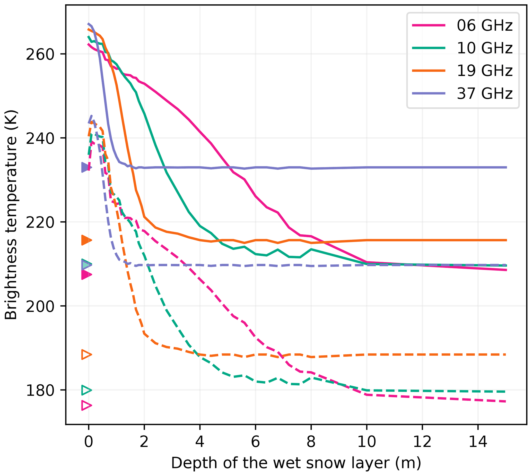
Figure 11 Brightness temperature of a wet snowpack as a function of the depth of a 10 cm thick wet snow layer at Roi Baudouin at V-pol (solid curves) and H-pol (dashed curves). Each curve is the average of the 100 best snowpacks to smooth the curves. The values of the dry brightness temperatures are marked by the triangles.

If we exclude a local maximum near the surface at H-pol (due to the impedance matching reducing the reflectivity when dry snow covers the wet snow layer), the brightness temperature decreases as a function of depth and reaches an asymptotic value corresponding to the dry snowpack. The rate of decrease depends mainly on the frequency. The 37 GHz signal reaches the asymptotic value above 2 m, and this depth is about 4, 8 and 10 m at 19, 10 and 6 GHz. These depths are consistent with the typical e-folding depths estimated in the Antarctic dry snowpack (Surdyk, 2002; Picard et al., 2009), and the decreasing trend with frequency is explained by the increasing absorption and scattering coefficients with frequency. Figure 12 illustrates this behavior with observations from the Wilkins site. This site was selected because refreezing (or percolation) of meltwater is slow and regular, leading to a clearly visible slow relaxation of the brightness temperatures at 10 and 6 GHz (decreasing in exponential shape). In contrast, 19 and 37 GHz brightness temperatures rapidly decrease as soon as the surface meltwater refreezes in March and then slowly increases from April, especially at 37 GHz, due to the accumulation of fresh snow with fine grains over the summer layer composed of metamorphosed snow, with coarse grains. This area is known for the presence of aquifers (Montgomery et al., 2020; van Wessem et al., 2021).

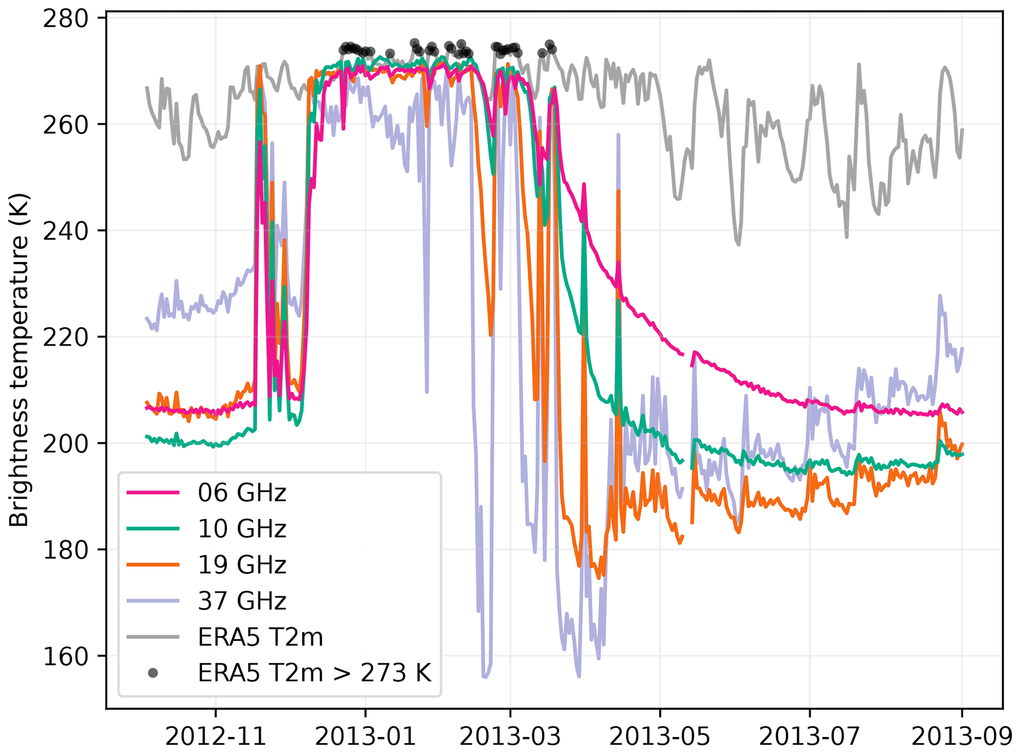
Figure 12 Time series of AMSR2 brightness temperature at V-pol and of ERA5 2 m air temperature (T2m) at Wilkins.

If we consider a detection threshold of 20 K above the dry mean H-pol brightness temperature, Fig. 11 indicates that wet snow can be detected at up to 5.6, 2.8, 1.4 and 0.6 m at Roi Baudouin for 6, 10, 19 and 37 GHz respectively. These values only partially follow the variations of e-folding depths with frequency because the detection is also dependent on the brightness temperature amplitude between dry and wet snow. This amplitude is lower at lower frequencies, and the detection is less sensitive in general.

Interestingly these detection depths are variable from site to site and depend on the season as depicted in Fig. 13. The site dependence seems to be influenced by the dry brightness temperature (Amery and Larsen C feature the lowest winter brightness temperatures at the two or three lowest frequencies and the deepest possible detection) rather than by the e-folding depth which is expected to be reduced when the brightness temperature is lower due to coarser snow grains. At 37 GHz the pattern is less marked, probably because of the reduced penetration depth because the snow in the topmost meter is new in winter and thereby not influenced by the previous year melt.

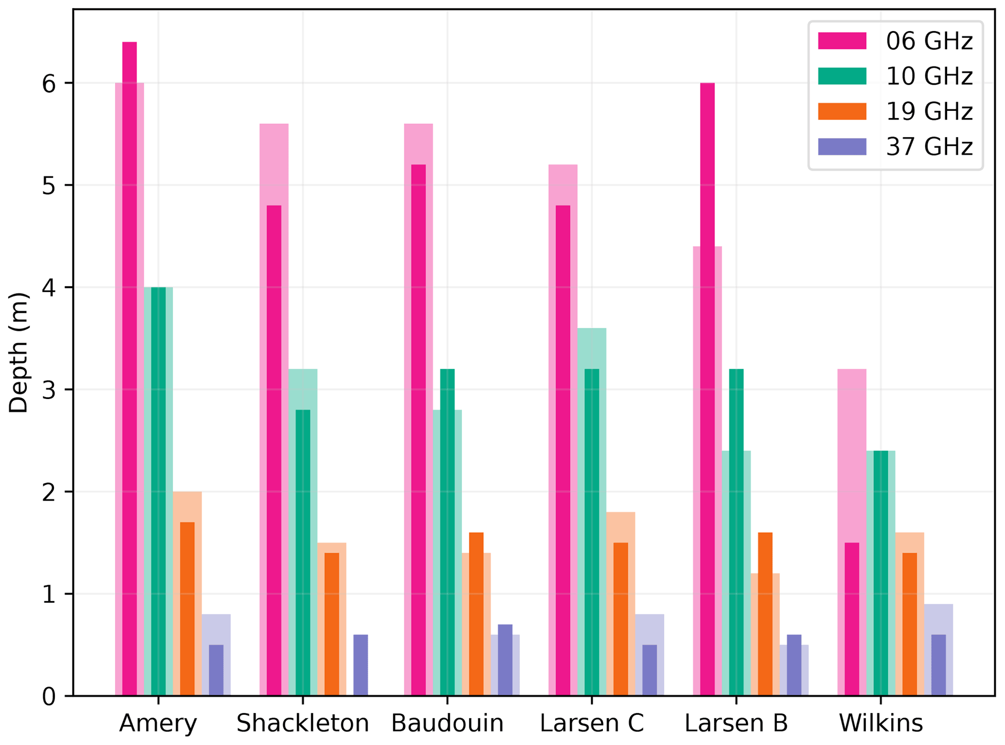
Figure 13 Maximum depth of detection (assuming a threshold at dry brightness temperature +20 K) as a function of season, site and frequency. The polarization is horizontal. Winter and autumn are in light- and dark-color shades respectively. Melt in Maudheimvida and Halvfarryggen is never detected with the aforementioned criterion.

The maximum detection depth is generally reduced in the autumn snowpack (dark-colored bars in Fig. 13) compared to that in winter (light-shaded bars). Meltwater profoundly transforms the upper snow layers by wet metamorphism and formation of ice nodules. Larger grains and nodules lead to enhanced scattering (when the snowpack becomes dry), which reduces the e-folding depth. The lower frequencies are less affected because these processes are most active near the surface and also because of the lesser role of scattering. This result implies that the detection at 37 GHz may be more challenging, with the necessity to adapt the threshold during the course of the melt season.

No maximum detection depth can be estimated for Maudheimvida and Halvfarryggen (the two driest sites) because the brightness temperature variations with the depth of the wet snow layer are much weaker than the threshold of 20 K and weaker than at the other sites (Fig. 14 for Halvfarryggen), probably because the dry snowpack is already close to a black body (small grains, high density, according to our retrieval). With a smaller threshold at these two sites, the melt could be detected in H-pol at low frequencies according to SMRT but not at high frequencies. This unexpected behavior is confirmed by the observed time series of brightness temperature in Fig. 14. The brightness temperature at 6 and 10 GHz features the characteristic increase of a melting snowpack in summer, although the higher frequencies follow the annual temperature cycle. The surrounding pixels (not shown) are alike, ruling out a collateral effect of the field of view increasing with decreasing frequency.

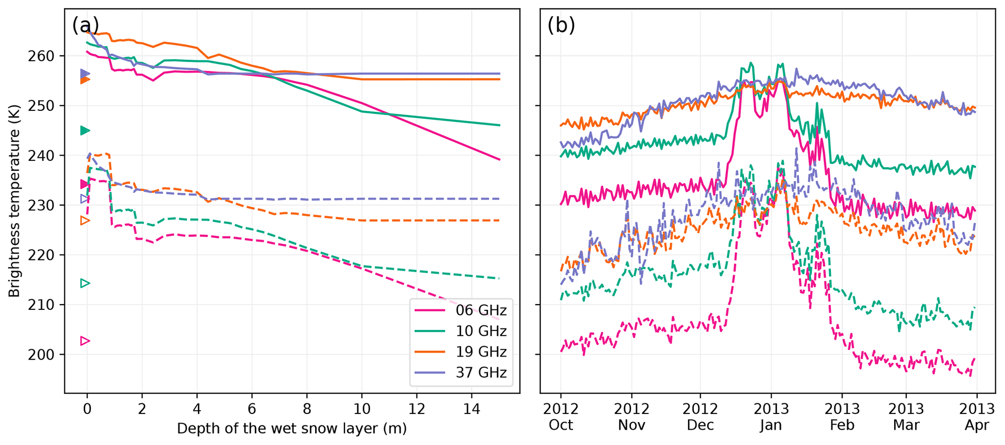
Figure 14 Brightness temperature as a function of the depth of the 10 cm thick wet snow layer at Halvfarryggen at V-pol (solid curves) and H-pol (dashed curves) (a). Values of dry brightness temperatures are marked by triangles. Each curve is the average of the 1000 best snowpacks. Time series of brightness temperature observations at Halvfarryggen (b).

4.5 Saturated snow layer (“slush”) and supraglacial lakes – Experiment 4

In Experiment 1, we evaluated the influence of the water content for small to moderate fractions (up to 20 kg m⁻², which is equivalent to 20 % water volume) and showed a decrease of H-pol brightness temperature in the reflective regime. In the case of intense melt and multiple freeze–thaw cycles, an impermeable ice horizon may form at or below the surface. By preventing percolation, this horizon allows for meltwater to accumulate, leading to high fractional volumes of water, which is often referred to as “slush” in the literature and is frequent in Antarctica (Dell et al., 2021). In the most extreme case, a supraglacial lake may form (no ice crystals are present at the surface). As soon as the thickness of such a saturated layer exceeds a quarter of the wavelength (Wiesmann et al., 1998), i.e., a few millimeters depending on the frequency, the brightness temperature strongly decreases due to the high reflectively of this layer. Here we investigate the risk of misclassifying such a pixel as not melting, despite the obvious presence of meltwater. Two cases are studied: a snow layer saturated with water (slush) and supraglacial lakes.

Saturated snow is modeled as a mixture of ice scatterers in a water background. Figure 15 shows the variations of brightness temperatures when the proportion of water increases from pure ice to pure water. When this layer is exactly at the surface (solid lines), the brightness temperature first increases (due to the increasing absorption) and then decreases to very low values (due to the increasing reflectivity of the wet interface). Analysis of the AMSR2 dataset suggests that such values, which are much lower than the winter average, have never been observed on glacial ice (it is however common on sea ice), which raises the question as to how realistic this simulation is.

Another set of simulations with the saturated layer overlaid by a thin moderately wet snow layer (5 cm thick and total water content of 5 kg m⁻²) was run (dashed lines in Fig. 15). The signal is completely different from the previous simulation because the wet snow layer is a strong absorber, so no radiation emerges from the saturated layer below, and its emission is close to that of a black body, so it has a high brightness temperature. These simulations highlight the critical role of the surface conditions. If the snow is wet but not saturated in the upper snowpack (a thickness of a quarter wavelength is sufficient), this layer and everything below have no influence on the brightness temperature.

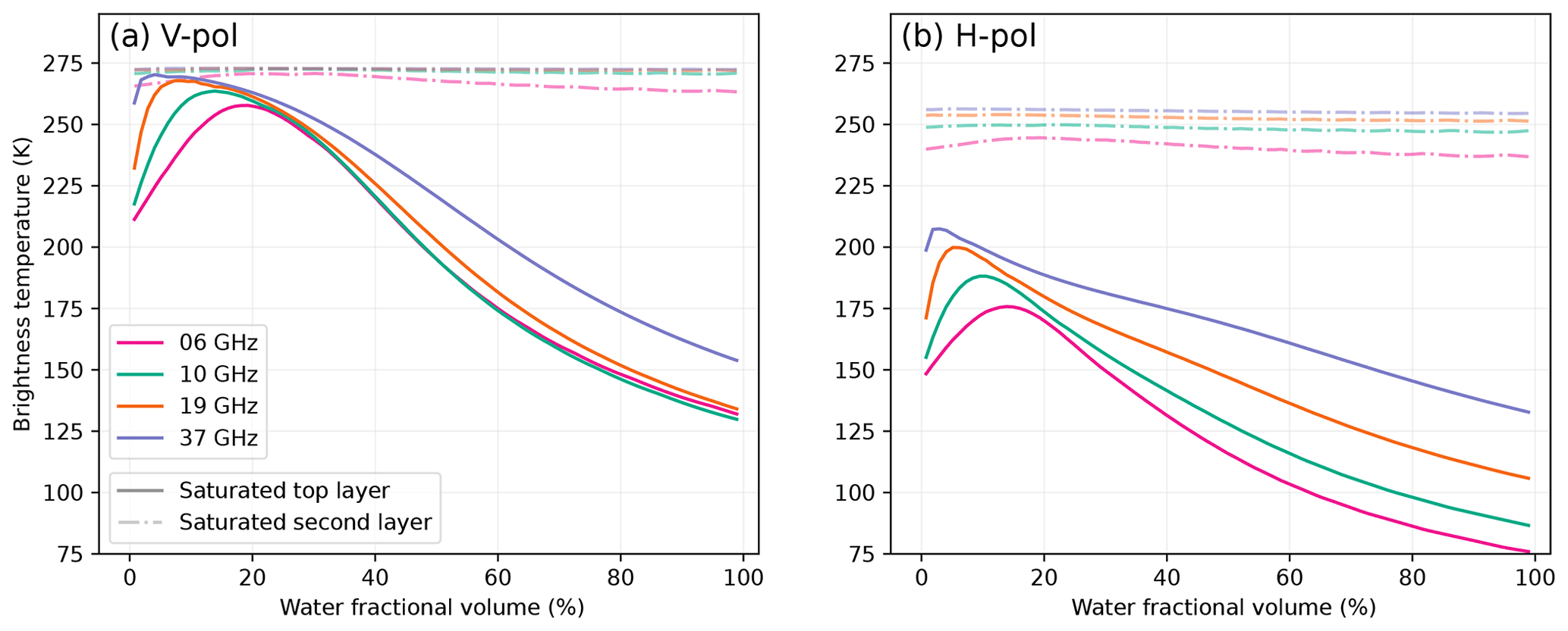
Figure 15 Brightness temperature of a water-saturated layer as a function of the water proportion (the remaining proportion is ice). The saturated layer is located at the top of the snowpack (solid lines) and 5 cm below a wet snow layer (5 kg m⁻², dashed lines).

Supraglacial lakes correspond to a water fractional volume of 100 % in Fig. 15, characterized by very low brightness temperatures. However, the coverage of supraglacial lakes is never complete at the scale of the microwave radiometer resolution (≈12–50 km) in Antarctica; a pixel contains some fraction of ponded lake water, and the remaining area is snow. To investigate this situation, which is frequent on the ice shelves, we simulate the pixel-averaged brightness temperature by linear combination of a simulation with a flat, pure-water surface and a simulation with a wet snowpack with 1.5 kg m⁻² total water content as in Experiment 1. The results in Fig. 16 show a strong negative trend in brightness temperature as a function of supraglacial lake fraction at both polarizations. When this trend intersects the threshold of detection (shown as a dashed horizontal line for each frequency and polarization, assuming the threshold at dry brightness temperature +20 K), the mixed pixel is detected as non-melting, which is a false negative. This occurs for lake fractions larger than 42 %–48 % at 6 GHz and 57 %–60 % at 19 GHz, the lower and higher bounds corresponding to the H-pol and V-pol respectively. Such high areal lake coverage fractions have rarely been observed in Antarctica (Arthur et al., 2022). For example, even before the near-complete collapse of the Larsen B Ice Shelf in 2002, which has been attributed to the hydrofracture drainage of about 3000 lakes (Banwell et al., 2013; Robel and Banwell, 2019), the fractional lake coverage reached a maximum of only 10 % (Banwell et al., 2014). Searching for a significant decrease in brightness temperature in the AMSR2 dataset has been unsuccessful even on shelves subject to ponding, as for instance on the north George VI Ice Shelf where a maximum of 15 % lake coverage was observed (Banwell et al., 2021) or on the eastern Roi Baudouin Ice Shelf (Dell et al., 2021).

We can conclude that false-negative melt detection due to supraglacial lake is unlikely at the present time in Antarctica. In contrast, the Greenland Ice Sheet is subject to more intense surface melting in the ablation area (Bell et al., 2018). For example, a recent case of flooding on the ice sheet was reported in August 2021 (Box et al., 2022) after an atmospheric river, combined with rain, triggered a massive melt event. The decrease in brightness temperature at 19 GHz is visible, although the surface was probably wet and remained wet for many days after this event.

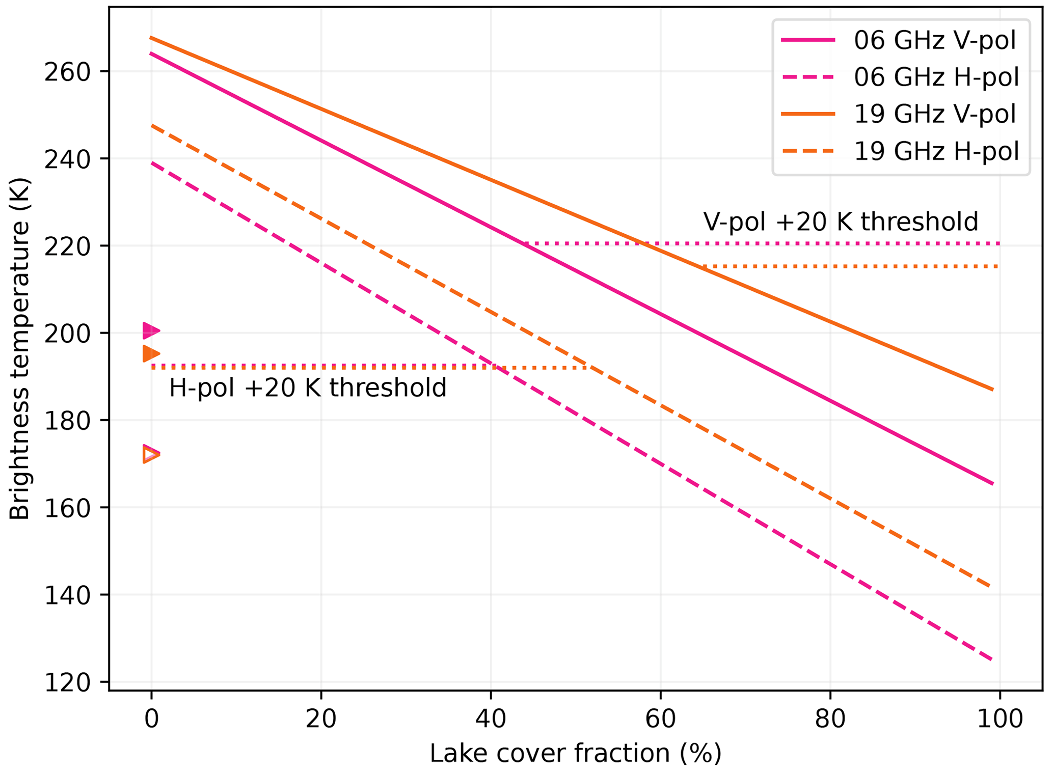
Figure 16 Brightness temperature of a mixed pixel as a function of lake cover fraction (the remaining area is covered by wet snowpack; 10 cm thick snow with 15 kg m⁻² of total water content). The dry winter brightness temperatures are indicated (triangles) as well as the thresholds of melt detection (dotted horizontal lines). Note that the H-pol thresholds are very close at both frequencies, with the lines almost overlapping.

4.6 The sensitivity of the L band to liquid water

Using the grain size adjusted snowpack, we assess the sensitivity of the L band to liquid water, first in the top layer with a similar setup as Experiment 1, except that the wet layer is 30 cm thick to account for the much longer wavelength at the L band. The analysis is conducted at Roi Baudouin where the dry snowpack simulations are fairly good (Fig. 3). Figure 17 highlights the overall lower sensitivity at the L band compared to the higher frequencies; the increase in brightness temperature is lower (15–25 K), and the maximum at V-pol is reached for a larger water amount (23 kg m⁻²). The H-pol reaches its maximum around 6.5 kg m⁻², which is 10 times the amount observed for the higher frequencies. This weaker sensitivity explains why lower thresholds have been used for the detection of melt with SMOS, as well as why a slightly adapted algorithm has been used (Leduc-Leballeur et al., 2020). This lower threshold does not imply larger detection errors because the brightness temperature during the dry periods is very stable throughout the year at the L band (Macelloni et al., 2016; Leduc-Leballeur et al., 2020). Hence even a change of ≈10 K is significantly larger than the noise level and the temperature-induced variations of brightness temperature.

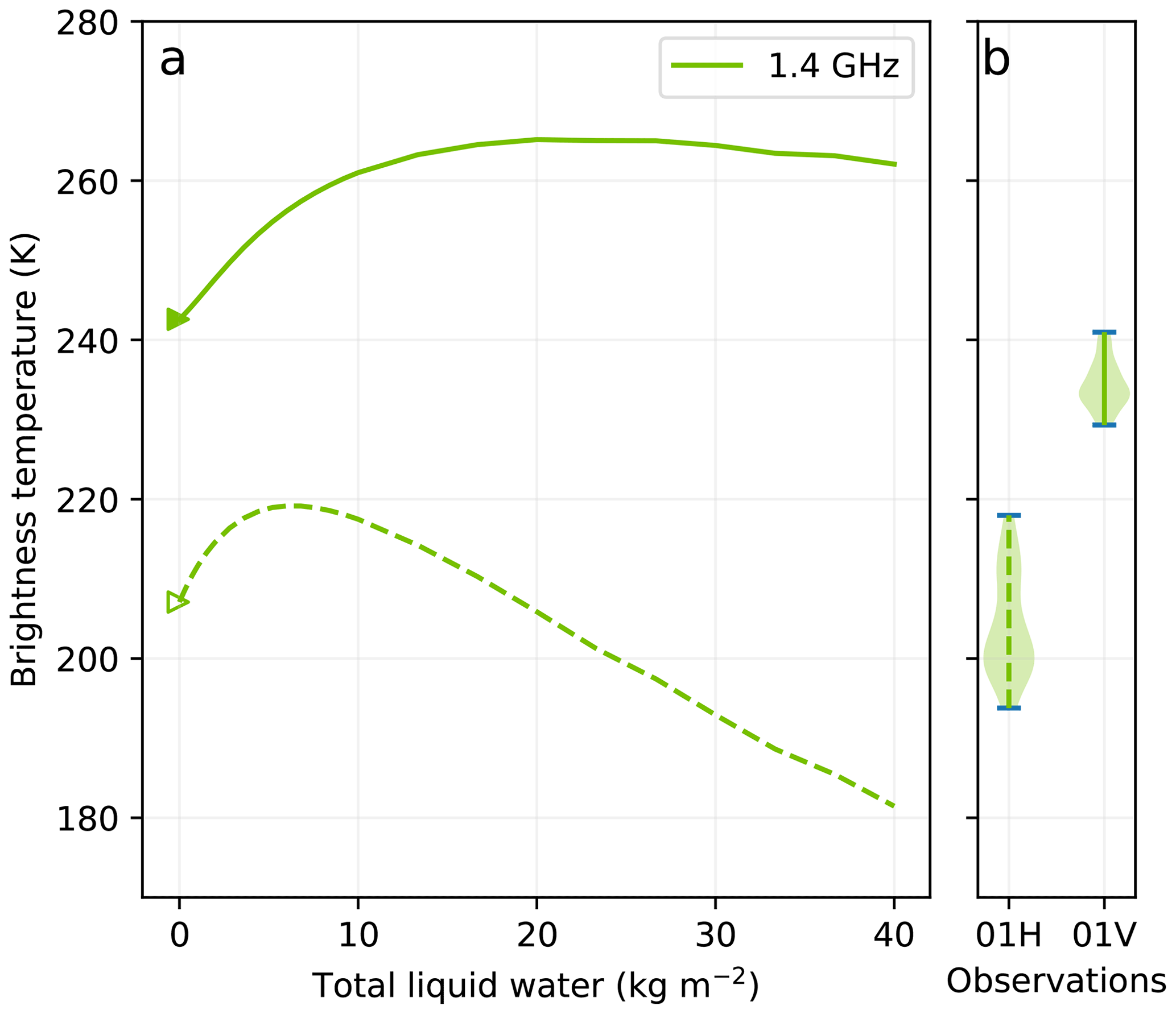
Figure 17 Brightness temperature at Roi Baudouin as a function of the total liquid water content in the top 30 cm of the snowpack at the L band at V-pol (solid) and H-pol (dashed) (a). The simulated dry brightness temperatures are marked by the triangles. Distribution of observed brightness temperature when the surface is melting according to Jakobs et al. (2020) (b).

According to the very low values of ice absorption at the L band (Mätzler, 1996; Macelloni et al., 2016, 2019), a wet snow layer could contribute to the radiation emanating from the snowpack up to depths of hundreds of meters. This is in apparent contradiction with the results in Fig. 18 showing the brightness temperature at the L band with a 30 cm thick wet snow layer (total water content of 14 kg m⁻²) at increasing depths (Experiment 3). The brightness temperature decreases within a few meters and reaches an asymptotic value. This value is relatively close to the dry brightness temperature (211 versus 207 K), making the melt detection difficult unless a very low threshold is used. This rapidly vanishing wet signature is due to the fact that the firn at the L band at depth is only weakly scattering so that both the wet snow layer and the firn at depth behave as a black body at a similar temperature; i.e., they emit the similar radiation flux. In the case where the firn temperature is significantly lower than 273 K (cold site), the asymptotic value may be higher than the winter (cold) brightness temperature and the detection at greater depths may be easier.

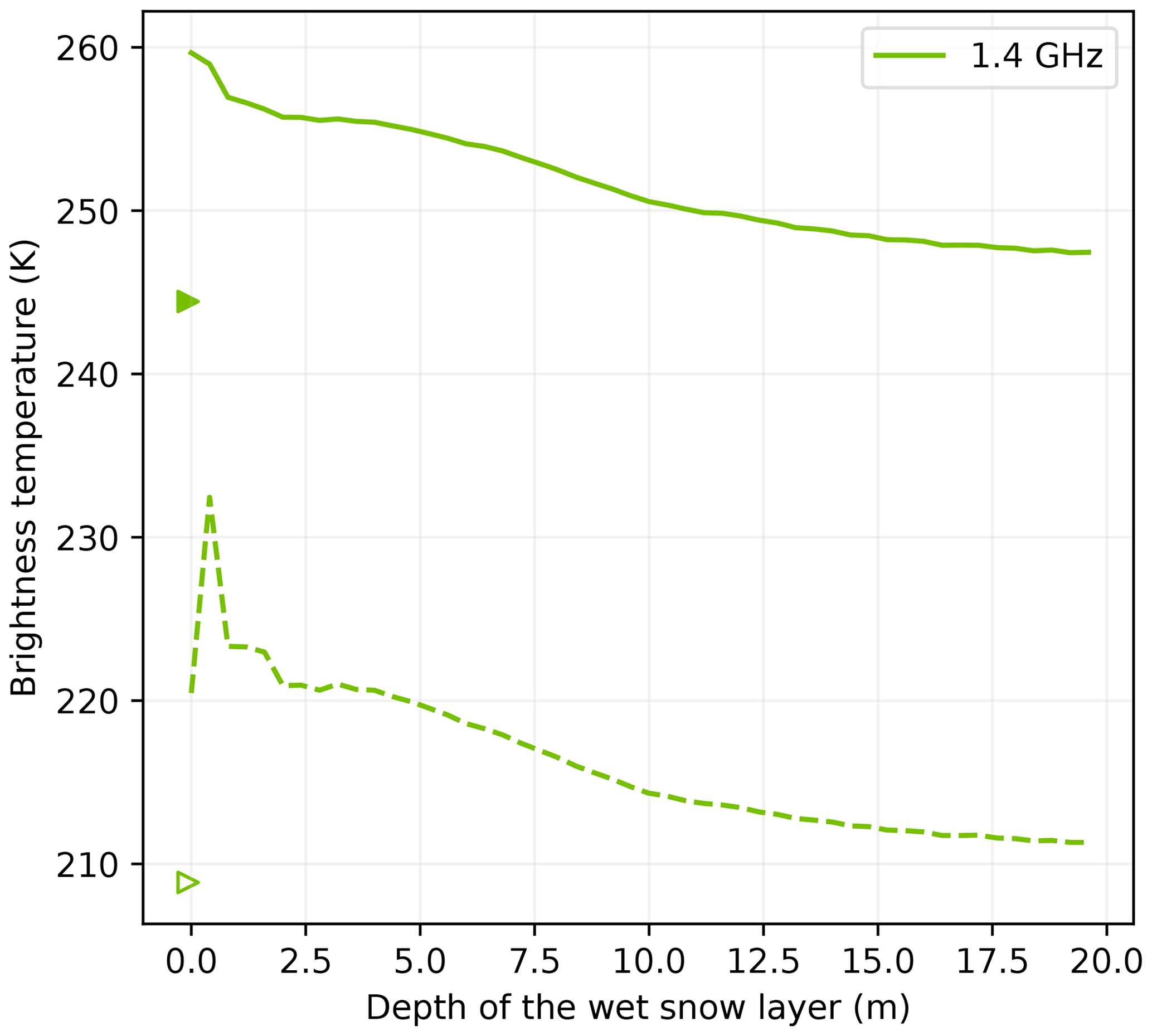
Figure 18 Brightness temperature at Roi Baudouin as a function of the depth of the 30 cm thick wet snow layer at the L band at V-pol (solid) and H-pol (dashed). The simulated dry brightness temperatures are marked by the triangles.

Figure 18 also shows a rapid increase in brightness temperature at H-pol between the top wet surface (213 K), as in Experiment 1, and just below the surface (235 K) (i.e., covered by a dry snow layer). The impedance matching is the cause (i.e., the reflectivity of the surface is lower when covered by dry light snow), and the consequence is that wet snow may be easier to detect when slightly buried than when right at the surface. Overall, the detection of liquid water at the L band is more difficult than for higher frequencies but possible at greater depths.

5 Discussion and conclusions

From the perspective of the algorithm developers and the users of melt products, three important knowledge gaps can be addressed with our results and analyses.

The minimum liquid water content required for microwave radiometry to detect the presence of meltwater is generally small compared to the melt amount produced over a typical summer day in Antarctic coastal areas (Jakobs et al., 2020). Even a small melt event is likely to be detected, especially with AMSR-E or AMSR2 which have an overpass time of near local noon (Picard and Fily, 2006). In contrast, the detection at the L band requires more water over a greater depth of snow. This result is confirmed in the observations (Leduc-Leballeur et al., 2020) but is subject to caution, because our simulations of the dry snowpack are not very accurate for the L band, due to a poor representation of large scatterers in the snowpack (probably ice pipes).

For a fine analysis of the melt products, estimation of a precise minimum liquid water content for detection might be necessary. Unfortunately, this threshold depends on many variables: the algorithm parameters (e.g., the brightness temperature threshold), the wave frequency and polarization, the preexisting snowpack properties (density and grain size near the surface), and more importantly the spatial distribution of liquid water within the sensor field of view (melt heterogeneity). Some of these variables are known a priori (e.g., sensor configuration), and their effect can be simulated by our modeling framework, but some others are subject to high uncertainties, resulting in uncertain minimum liquid water content values. To evaluate firn models against microwave-derived melt products, the usual current practice is to assume a fixed minimum water content (Fettweis et al., 2011; Kuipers Munneke et al., 2012). Instead, we suggest the exploration of a range of minimum water content between, e.g., 0.2 and 1 kg m⁻² to test the significance of the results. For instance, a model showing a systematic positive bias for a large range of minimum water contents is clearly positively biased. On the other hand, a bias with changing sign when the minimum water content is varied would indicate that the model is not biased and is as good (or uncertain) as the melt product. For the algorithm developers, we suggest providing outputs with varying parameters, as for instance in Banwell et al. (2021), where the brightness temperature threshold used to detect melt was varied in a reasonable range (i.e., from 2.5 to 3.5× the standard deviation of the winter brightness temperature) to give a rough uncertainty estimations for the annual number of melting days.

The maximum snow depth for liquid water detection is another important parameter to enable the accurate use of microwave radiometer melt products. For instance to compute the “total” liquid water in a firn model, outputs must be evaluated from the surface to this depth. The main factor controlling this depth is the frequency, with variations from 0.1–0.2 m at 37 GHz to about 10 m at 1.4 GHz. Taking advantage of this large depth range to provide rich information on surface refreezing and percolation is an important research avenue (Leduc-Leballeur et al., 2020; Miller et al., 2020; Colliander et al., 2022). The preexisting snowpack properties (density, grain size and ice layers) are a secondary factor modulating this maximum depth, and since all these properties evolve rapidly in wet conditions, the depth is subject to seasonal variations. We have shown that the retrieval of these three snow properties is feasible before and after the melt season, but the wet snowpack remains opaque during the melt season, forbidding the retrieval of any information under the wet layer. Additionally, as a general rule, the maximum depth of detection decreases slightly over the course of a melt season due to grain coarsening, densification and ice layer formation that occur in wet conditions.

The two regimes of variations in the brightness temperature result in non-monotonic variations as a function of liquid water content. This could be an issue for melt detection as very wet snow has a low brightness temperature (especially at H-pol), potentially below the melt detection threshold. Our results show that the required amount of water concentrated in the upper layer is large and is not typical of the Antarctic environment at the present time. While the H-pol is often favored over the V-pol for melt detection (Zwally and Fiegles, 1994; Tedesco et al., 2006; Torinesi et al., 2003b), future algorithms could assess the benefit of using V-pol brightness temperature to mitigate this problem versus the disadvantage of the lower V-pol contrast between dry and wet conditions. Finally, in the reflective regime, for liquid water contents higher than 2–5 kg m⁻², the H- and V-pol signals can be used to retrieve liquid water content (Naderpour and Schwank, 2018; Houtz et al., 2021), but we have shown that appropriate prior knowledge of the surface density and absence of water at depth are essential.

Geographically, our study relies on specific sites in Antarctica's coastal areas, mainly ice shelves. However, most results show relatively small inter-site variations, which leads us to conclude that the benefit of this study is more general and contributes to the knowledge of the Antarctic Ice Sheet at large. Applicability to the accumulation area of the Greenland Ice Sheet (where the glacial ice is far below the microwave penetration depth) and where the number of melting days is similar is probably acceptable. In addition, despite using AMSR2 and SMOS observations, our results also apply to any radiometric sensor operating at frequencies of 1.4–37 GHz and with incidence angles of 50–60^∘. This includes for instance SMMR (Scanning Multi-channel Microwave Radiometer), SMAP, SSM/I (Special Sensor Microwave/Imager), SSMIS (Special Sensor Microwave Imager/Sounder) and CIMR.

This work has provided the basis for developing new advanced melt detection algorithms, a logical future avenue of research. However, we stress that fundamental knowledge is still missing regarding the wet snow permittivity, the small-scale liquid water variability and the snowpack properties in the coastal Antarctic environment, particularly on the ice shelves. Future work should focus on filling these gaps given the growing importance of the ice sheet hydrology as the climate warms.