Changes in the annual sea ice freeze–thaw cycle in the Arctic Ocean from 2001 to 2018

The annual sea ice freeze–thaw cycle plays a crucial role in the Arctic atmosphere—ice–ocean system, regulating the seasonal energy balance of sea ice and the underlying upper-ocean. Previous studies of the sea ice freeze–thaw cycle were often based on limited accessible in situ or easily available remotely sensed observations of the surface. To better understand the responses of the sea ice to climate change and its coupling to the upper ocean, we combine measurements of the ice surface and bottom using multisource data to investigate the temporal and spatial variations in the freeze–thaw cycle of Arctic sea ice. Observations by 69 sea ice mass balance buoys (IMBs) collected from 2001 to 2018 revealed that the average ice basal melt onset in the Beaufort Gyre occurred on 23 May (±6 d), approximately 17 d earlier than the surface melt onset. The average ice basal melt onset in the central Arctic Ocean occurred on 17 June (±9 d), which was comparable with the surface melt onset. This difference was mainly attributed to the distinct seasonal variations of oceanic heat available to sea ice melt between the two regions. The overall average onset of basal ice growth of the pan Arctic Ocean occurred on 14 November (±21 d), lagging approximately 3 months behind the surface freeze onset. This temporal delay was caused by a combination of cooling the sea ice, the ocean mixed layer, and the ocean subsurface layer, as well as the thermal buffering of snow atop the ice. In the Beaufort Gyre region, both (Lagrangian) IMB observations (2001–2018) and (Eulerian) moored upward-looking sonar (ULS) observations (2003–2018) revealed a trend towards earlier basal melt onset, mainly linked to the earlier warming of the surface ocean. A trend towards earlier onset of basal ice growth was also identified from the IMB observations (multiyear ice), which we attributed to the overall reduction of ice thickness. In contrast, a trend towards delayed onset of basal ice growth was identified from the ULS observations, which was explained by the fact that the ice cover melted almost entirely by the end of summer in recent years.

1 Introduction

Seasonal thermodynamic freezing and thawing processes are crucial to controlling the mass budget of the cryosphere (Planck et al., 2020; Derksen et al., 2012). In the Arctic Ocean, the presence of sea ice greatly modifies the exchanges of heat, momentum, and mass between the atmosphere and the ocean. The timings of the sea ice melt and freeze onsets, as well as the length of the melt and freeze seasons, play a key role in the heat budget of the atmosphere–ice–ocean system. For example, they alter the surface albedo and meltwater budget in summer (Perovich and Polashenski, 2012; Stroeve et al., 2014) and the brine discharge in both winter (Ivanov et al., 2016) and summer (Tian et al., 2018) through different mechanisms. Changes in the lengths of the melt and freeze seasons also regulate the degree of consolidation and mechanical strength of the sea ice cover and consequently enhance or weaken the mobility and deformation of the sea ice, even if the wind forcing does not change (Rampal et al., 2019; Lei et al., 2021). Passive microwave (PMW) satellite observations indicated that the length of the sea ice surface melt season is extending with a rate of 5 d per decade due to both earlier melt onset and later freeze onset, especially in the peripheral seas where seasonal sea ice dominates (Stroeve et al., 2014). Lengthening of the melt season leads to more solar energy absorption and storage in the ice–ocean system (Perovich et al., 2011), contributing to the thinning and loss of Arctic sea ice in summer (Perovich and Richter-Menge, 2015), promoting the bloom of ice algae and phytoplankton under the ice (Ardyna and Arrigo, 2020) and suppressing the ice recovery in winter (Timmermans, 2015; Ricker et al., 2021). Thus, the melt and freeze onsets can be considered significant phenological indices of the Arctic climate system.

The majority of related studies have derived the phenological indices of the Arctic melt and freeze onsets based on observations of the ice surface (hereafter refer as SMO and SFO), such as in situ, reanalyzed, or remotely sensed near-surface air temperature (Rigor et al., 2000; Bliss and Anderson, 2018); passive microwave brightness temperature (Markus et al., 2009; Stroeve et al., 2014; Bliss et al., 2017); active microwave backscatter from scatterometers (Drinkwater and Liu, 2000; Wang et al., 2011); and synthetic aperture radar (Mahmud et al., 2016; Howell et al., 2019). Despite the differences between the various data sources and methodologies, all of them have consistently revealed a statistically similar long-term trend towards earlier SMO and delayed SFO (Markus et al., 2009; Bliss et al., 2017; Bliss and Anderson, 2018). In situ observations obtained during the Surface Heat Budget of the Arctic Ocean (SHEBA) experiment in the Beaufort Gyre region in 1997–1998 revealed that the SMO and SFO were primarily driven by pronounced atmospheric synoptic events, with specific dates triggered by a rain-on-snow event and a sequence of cold front passages, respectively (Persson, 2012). The SMO usually starts due to a large increase in downwelling longwave radiation and is accompanied by moderate decreases in the surface albedo, while the SFO initiates after a step-like decrease of the net surface energy flux (Persson, 2012). Reanalysis data also indicated that downwelling longwave radiation is the main factor in determining the variability of the SMO (Maksimovich and Vihma, 2012). Numerical simulations showed that positive anomalies of downward longwave radiation in spring and early summer initiated an earlier SMO (Kapsch et al., 2016).

The freeze–thaw cycle at the bottom of sea ice is much different from that at the ice surface due to the additional regulation of the heat balance by the heat flux from the ocean (Lei et al., 2018). In the Beaufort Gyre region, the amount of summer sea ice basal melt is generally comparable to or even larger than the surface melt (Perovich and Richter-Menge, 2015; Planck et al., 2020). The brine or freshwater injection associated with ice basal freezing and thawing processes is the main mechanism altering not only the physical hydrographic environment (Jackson et al., 2010; Randelhoff et al., 2017) but also the ecosystem (Ardyna and Arrigo, 2020; von Appen et al., 2021) of the underlying ocean. Despite their importance, the complete freeze–thaw cycle, as well as the onset of basal ice melt and basal ice growth (BMO and BFO), cannot be directly determined by any remotely sensed radar or laser altimeter because of the difficulty in differentiating between sea ice and open water leads due to the impact of melt ponds in the summer melt season (Laxon et al., 2013; Kwok et al., 2018).

The sea ice freeze–thaw cycle can be identified using measurements from sea ice mass balance buoys (IMBs), which consist of a thermistor chain in combination with acoustic sounders above and below the ice, and can provide sea ice mass balance observations from both the ice surface and ice base at a single point on a given ice floe (Perovich et al., 2021). Using such instruments, both surface and basal melt/freeze onsets as well as freeze–thaw cycles can be obtained at the measurement site along the Lagrangian drifting trajectory of the ice. Though IMBs are limited to one-dimensional ice mass balance measurements on individual ice floes, the deployment site is usually chosen in an area of undeformed sea ice which is ideally representative of the ice conditions in a greater area (Planck et al., 2020). During the SHEBA campaign, IMB observations of undeformed ice at the Quebec 2 site in 1998 indicated that the surface melt was initiated by a rain-on-snow event on 29 May and ended by 17 August, while basal melt began in early June and ended in early October (Perovich et al., 2003). Planck et al. (2020) found that the BMOs at eight IMB sites in the Beaufort Gyre from 1997 to 2015 occurred within a relatively narrow window of 13 d in early June and suggested some potential explanations such as warm water advection from the Bering Sea and the ice basal energy budget. Based on measurements obtained by an “Ice-T” buoy deployed at the North Pole Environmental Observatory (NPEO) campaign in 2011, Vivier et al. (2016) found that the observed BMO in the central Arctic Ocean preceded the SMO by 20 d. They ascribed this to increased solar heating of the upper ocean through opening leads caused by storm events, highlighting the influence of synoptic events not only on freezing and thawing processes on the sea ice surface but also on those occurring at the ice bottom.

Another method to identify the sea ice freeze–thaw cycle is using data provided by upward-looking sonars (ULS), which are usually deployed at the top of moorings in fixed geographic locations, measuring the submerged portion of the sea ice (ice draft). The ice draft can be converted to total sea ice thickness using an assumed ratio of ocean to ice densities and also taking snow depth atop the ice into account (Krishfield et al., 2014). Analyzing the evolution of the probability distribution of the ice draft obtained from the ULS record in the Beaufort Gyre from 2003–2012, Krishfield et al. (2014) identified distinct seasonal cycles of sea ice thermodynamic growth and decay. Thus, the ULS measurements are a suitable tool for detecting the melt and freeze onsets defined by the thermodynamic processes (Smith and Jahn, 2019).

In essence, the basal melt and growth onsets are controlled by the heat balance at the ice–ocean interface, which is related to the thermodynamics of both sea ice and the upper ocean. During several field campaigns, ice-tethered profilers (ITPs) were co-located with IMBs to simultaneously monitor the thermodynamic processes related to the ice and the underlying ocean (Toole et al., 2011). On a seasonal scale, the oceanic heat flux to the ice can be derived from two methods, i.e., by the sub-ice ocean water properties as measured by the ITP (Timmermans et al., 2011; Zhong et al., 2022) and by sea ice temperature and thickness changes derived from an IMB (Lei et al., 2018). A comparison of both measurements has so far shown good agreement for the melting and freezing seasons in both the Arctic and Antarctic (Timmermans et al., 2011; Ackley et al., 2015).

In this study, we mainly focus on the characterization of the spatiotemporal variations in the ice surface and basal melt and freeze onsets in the Arctic Ocean by combining data from historical IMBs, passive microwave remote sensing, and ULS measurements. Further taking into account reanalysis data, we investigate the changes of surface radiation during the transition between freeze and thaw cycles. By co-analyzing IMB and ITP data, we also explore the connection of the basal melt and growth onsets with heat fluxes from the surface and upper ocean. Based on our analysis, long-term variations in the patterns of the sea ice freeze–thaw cycle and their regional differences are revealed, and the coupling mechanisms between the sea ice melt–freeze cycle with the lower atmosphere and upper ocean are discussed.

2 Data and methods

2.1 Data

2.1.1 Ice mass balance buoys

The main data sources for this paper are the more than 100 ice mass balance buoys (IMBs) and seasonal ice mass balance buoys (SIMBs) designed by the Cold Regions Research and Engineering Laboratory (CRREL, Hanover, New Hampshire) that have been deployed in the Arctic Ocean since 2000 (Perovich et al., 2022). In this paper, we refer to both types as IMB for simplicity. Each IMB is named by the year of deployment and followed by one letter in alphabetical order. The spatial coverage of the IMBs mainly extends into the central Arctic Ocean (CAO, roughly located north of 80^∘ N and with a bathymetry deeper than 1000 m) and the Beaufort Gyre (BG, roughly located between 70 and 80^∘ N, 130 and 170^∘ W with bathymetry deeper than 300 m). The IMBs deployed on landfast ice are excluded from this study because shallow coastal waters have different ice–ocean coupling mechanisms and are more vulnerable to terrigenous heat and freshwater inputs (Eicken et al., 2005). The acoustic sounders on the IMBs measure the distance to the ice surface and ice base with a resolution of ±1 cm (Planck et al., 2020). Thus, both melt and freeze onsets of the ice surface and ice base at the deployment sites can be identified with high reliability. The surface melt and freeze onsets can also be related to near-surface air temperature (Rigor et al., 2000). Additionally, a thermistor chain with a vertical resolution of 0.1 m provides temperature profiles through air, snow, ice, and ocean at an accuracy of 0.1 ^∘C, which can be used for an analysis of the sea ice basal energy balance. In total, 69 IMBs are used in this study to detect the ice surface and/or basal melt and freeze onsets in the BG and CAO for the period 2001–2018 (Fig. 1).

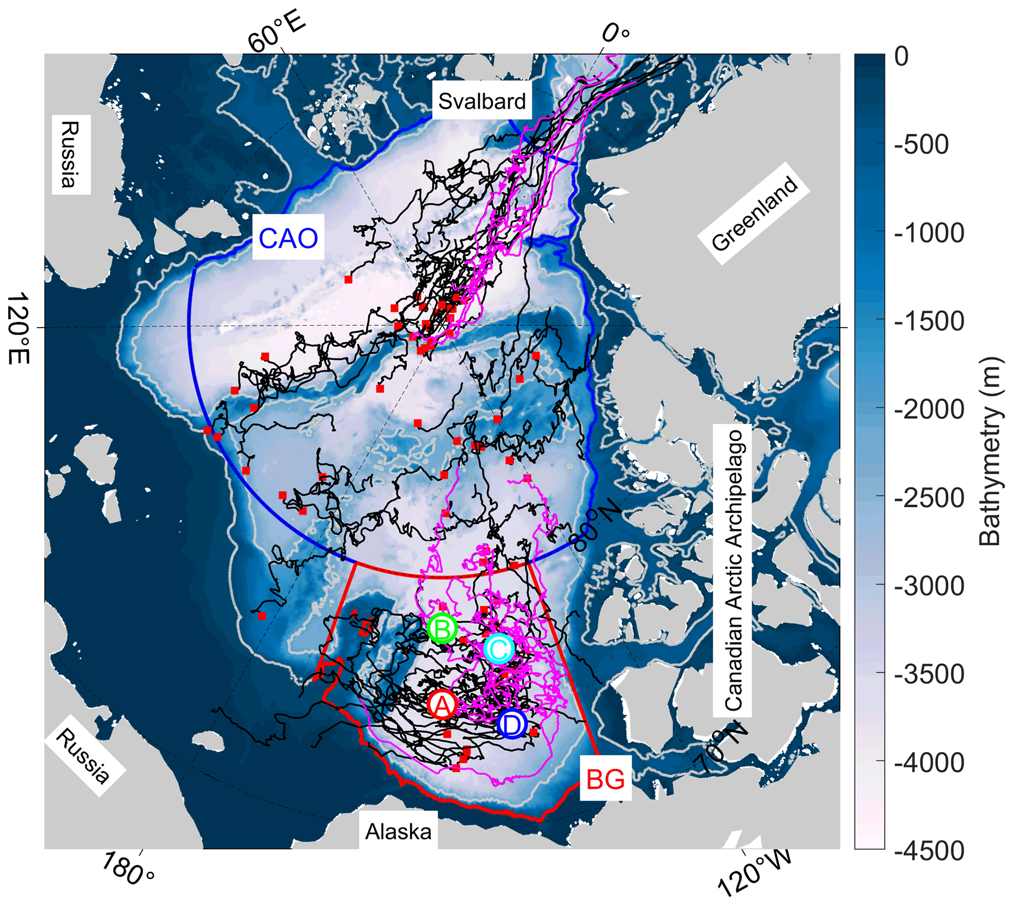
Figure 1 Deployment locations (red squares) and drift trajectories (solid lines) of 69 IMBs deployed in the Arctic Ocean in 2001–2018. The pink lines are drifting trajectories of IMBs co-located with ITPs. The locations of four moored ULSs in the Beaufort Gyre Observation System are indicated by BGOS-A, B, C, and D. The Beaufort Gyre and the central Arctic Ocean are defined by the areas with red and blue boundaries, respectively. The color map indicates the bathymetry from the 2 min Gridded Global Relief Data (ETOPO2) v2 distributed by NOAA National Centers for Environmental Information (https://doi.org/10.7289/V5J1012Q, NOAA National Geophysical Data Center, 2006). Grey contours depict the −300 and −2000 m bathymetry.

2.1.2 Upward-looking sonar data

Three to four upward-looking sonars (ULSs) were installed at the top of several moorings deployed beneath the BG sea ice as parts of the Beaufort Gyre Observation System (BGOS-A, B, C, and D) every year since 2003, providing year-round time series of ice draft (Proshutinsky et al., 2009). BGOS-A and BGOS-B were deployed along the 150^∘ W meridian at 75 and 78^∘ N, respectively. BGOS-C and BGOS-D were deployed along the 140^∘ W meridian at 77 and 74^∘ N, respectively (Fig. 1). After corrections for atmospheric pressure and speed of sound variations, the estimated error of the ice draft measurement is ±0.05–0.10 m (BGOS ULS Data Processing Procedure; Krishfield et al., 2014). Ice draft is scaled by a fixed ratio of the ocean-to-ice density (1.123) to convert to ice thickness. Since daily average of ice thickness tends to be strongly affected by deformed ice resulting from dynamic ridging and leads opening (Hansen et al., 2014), the daily median ice thickness is used to infer the thickness changes due to thermodynamic growth and decay, and subsequently to identify the timing of the ice annual freeze–thaw cycle (Krishfield et al., 2014).

2.1.3 Oceanographic data from ice-tethered profilers

Ice-tethered profilers (ITPs) designed by the Woods Hole Oceanographic Institution have been deployed in the Arctic Ocean since 2004 to autonomously measure upper-ocean properties at depths between ∼ 7 and 750 m (Krishfield et al., 2008a). The ITP measures seawater temperature, conductivity, and pressure at a frequency of 1 Hz. Temperature and derived salinity are vertically averaged into 2 dbar bins after the application of a standard data processing procedure (Krishfield et al., 2008b). Some ITPs were co-deployed with IMBs so that simultaneous measurements of seawater properties and sea ice basal freeze–thaw processes could be obtained. In this study, data measured by 12 ITPs (pink lines in Fig. 1) are used when either the basal melt or freeze onset is detected by the co-located IMB to investigate the coupling mechanism between the sea ice and the upper ocean. In addition, data from 17 ITPs deployed in the general area of the central BG are used to characterize the decadal changes in spring sea surface temperature, which can indicate the changes in the upper-ocean contribution to enhanced sea ice melt. Here, we focus on a narrow region to eliminate spatial differences as much as possible.

2.1.4 Ice surface melt and freeze onset from passive microwave data

The satellite PMW dataset of surface melt and freeze onset dates is available from the NASA Cryosphere Science Research Portal, gridded to 25 km × 25 km using an equal-area projection (https://earth.gsfc.nasa.gov/cryo, last access: 31 December 2021, Markus et al., 2009; Stroeve et al., 2014). Based on the emissivity change due to the presence of liquid water, this dataset incorporates the PMW melt and freeze onset algorithm applied to passive microwave brightness temperatures collected over the period 1979–2020 from the Nimbus-7 Scanning Multichannel Microwave Radiometer (SMMR), the Special Sensor Microwave/Imager (SSM/I); and the Special Sensor Microwave Imager/Sounder (SSMIS). The PMW dataset includes early melt and freeze onset dates, defined as the first day of ice surface melt or freeze, as well as continuous melt and freeze onset dates, defined as the day after which ice surface melting or freezing conditions persist. Here, we used these four records to identify the timing of ice surface melting or freezing at a given IMB location.

2.1.5 Sea ice concentration data

Daily sea ice concentration data are provided by the Advanced Microwave Scanning Radiometer for EOS (AMSR-E) and its successor AMSR2 brightness temperatures using the ARTIST sea ice (ASI) algorithm, with a spatial resolution of 6.25 km × 6.25 km under an equal-area projection (http://www.seaice.uni-bremen.de, last access: 31 December 2021, Spreen et al., 2008). To evaluate the impact of the shortwave radiation absorption by the ocean on sea ice freeze–thaw processes, a representative sea ice concentration around each buoy's location on a specific day is estimated by averaging the concentration value of pixels within a radius of 50 km around the respective buoy.

2.1.6 Atmospheric reanalysis data

The surface net shortwave and net longwave fluxes along the IMB trajectories are obtained from the European Centre for Medium-Range Weather Forecasts (ECMWF) ERA5 reanalysis dataset (Copernicus Climate Data Store, https://cds.climate.copernicus.eu, last access: 3 April 2022, European Centre for Medium-Range Weather Forecasts, 2019), which is produced using 4D-Var data assimilation and model forecasts in CY41R2 of the ECMWF Integrated Forecasting System. The ERA5 dataset extends from 1950 to 2020, with a horizontal spatial resolution of 0.25^∘ × 0.25^∘ and a temporal resolution of 1 h. For evaluation of the surface atmospheric energy budget over the ice related to the ice freezing–thawing processes, the ERA5 data are daily averaged and bilinearly interpolated to a respective buoy's position.

2.2 Methods

2.2.1 Detection of surface melt and freeze onsets

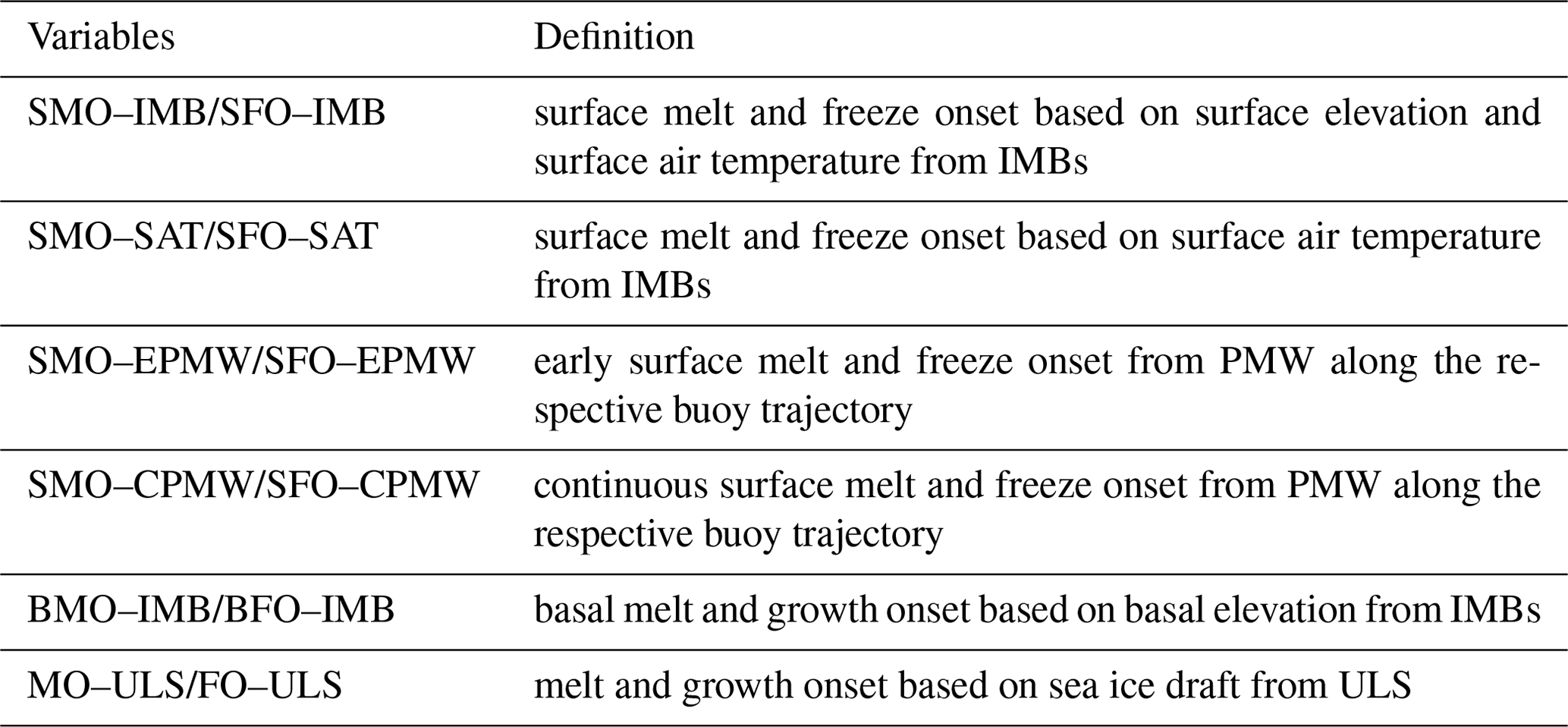
Three methods are applied for the detection of SMO and SFO. First, based on surface snow and ice mass balance observations and a combination of surface air temperature (SAT), SMO–IMB is defined as the date when the change of two subsequent daily records of surface position is negative, and the SAT is higher than −1 ^∘C. Correspondingly, the SFO–IMB is defined as the date when the ice surface stops melting, and the SAT drops below −1 ^∘C (i.e., from then on the ice surface is no longer melting). Second, the ice surface melt and freeze onsets are detected using SAT, which has been a widely adopted method. Here, based on the SAT measured by the IMB, SMO–SAT and SFO–SAT are defined as the dates when observed daily SAT rises or drops below a threshold temperature of −1^∘C after a 14 d running-mean filter is applied (e.g., Rigor et al., 2000; Bliss and Anderson, 2018). Third, early melt onset (ESMO–PMW), continuous melt onset (CSMO–PMW), early freeze onset (ESFO–PMW), and continuous freeze onset (CSFO–PMW) of each buoy location are derived from PMW satellite observation (Markus et al., 2009) along the respective buoy trajectory. However, the PMW data are not available in the vicinity of the North Pole due to the constrained satellite orbit.

2.2.2 Detection of basal melt and growth onsets using IMB and ULS data

The basal melt (BMO–IMB) and growth onsets (BFO–IMB) are identified from IMB observations as the date when the ice bottom elevation reaches the lowest (largest basal ice growth) or highest (largest basal ice melting) positions, respectively, after applying a 14 d running-mean filter. The potential interference in BFO–IMB detection caused by the formation of false ice bottoms (Eicken, 1994) in the melt season is carefully identified and excluded. When false ice bottoms exist, the IMB observations typically showed basal growth without any associated atmospheric and/or oceanic temperature signals, followed by a rapid thinning in early to mid-summer (Smith et al., 2022). In this case, the BFO–IMB is detected after the false-bottom formation. A second set of indices indicating ice basal melt and growth onsets is derived from ULS daily median ice draft data. The ULS measures the total ice draft, which is usually integrating both ice surface and basal melt and freeze processes. Thus, we cannot separate the changes in the ice surface and bottom using ULS data. However, we can obtain a total 1-D ice volume tendency from this dataset. First, the climatological ice thickness at each mooring site is derived to remove the irregularly fluctuating data from the time series to separate the modal ice from the ridged ice. Then, the MO–ULS and FO–ULS are defined as the dates when the smoothed ice thickness reaches the maximum or minimum value after applying a 30 d running-mean filter. When the sea ice has vanished completely in summer, FO–ULS is defined as the first day when a persistent ice cover is continuously observed.

Table 1 Definition of different surface and basal melt and freeze onsets.

2.2.3 Estimation of conductive heat flux and oceanic heat flux at the ice–ocean interface

To mitigate the effect of the highly porous skeletal layer near the ice base (Lei et al., 2014), the bulk conductive heat flux in the sea ice is investigated for a specified reference layer defined at 0.2–0.6 m above the ice base and estimated by

$$\begin{array}{}\text{(1)}& F_c=k_{\mathrm{i}}{\displaystyle \frac{\partial T_{\mathrm{i}}}{\partial z}},\end{array}$$

where k_i is the sea ice thermal conductivity and $\partial T_{\mathrm{i}}/\partial z$ is the vertical ice temperature gradient. k_i is a function of sea ice temperature and salinity (Untersteiner, 1961). According to McPhee (1992) and McPhee et al. (2003), the oceanic heat flux from the mixed layer into the sea ice primarily depends on the amount of surface mixed-layer heat, which is characterized by the ocean mixed-layer temperature departure from the freezing point (ΔT), as well as on the turbulent mixing in the boundary layer, characterized by the friction speed, u_*0. Operationally, ΔT is calculated using the topmost valid data from an ITP dataset, if that depth is shallower than 20 m. u_*0 is calculated as

$$\begin{array}{}\text{(2)}& {\displaystyle \frac{\mathit{\kappa }\mathit{V}}{{\mathit{u}}_{*\mathrm{0}}}}=\log {\displaystyle \frac{\left|{\mathit{u}}_{*\mathrm{0}}\right|}{f{z}_{\mathrm{0}}}}-A-iB,\end{array}$$

where V is the difference between ice velocity and surface geostrophic current velocity; f is the Coriolis parameter; z₀ is the hydraulic roughness of the ice bottom with a typical value of 0.01 m for undeformed multiyear sea ice; and A and B are constants with values of 2.12 and 1.91, respectively (McPhee et al., 2003). The geostrophic current velocity is relatively small in the Arctic pack ice zone, typically less than 5 cm s⁻¹, which can be neglected (Krishfield and Perovich, 2005). Then, the oceanic heat flux F_w is estimated as follows:

$$\begin{array}{}\text{(3)}& F_w={\mathit{\rho }}_{\mathrm{sw}}{c}_p{C}_{\mathrm{H}}{u}_{\ast \mathrm{0}}\mathrm{\Delta }T,\end{array}$$

where ρ_sw and c_p are the density and specific heat of seawater, respectively, and C_H=0.006 is a bulk heat transfer coefficient (McPhee, 1992).

3 Results and discussion

For each IMB trajectory, four pairs of surface melt and freeze onsets and one pair of basal melt and growth onsets are derived (Table S1). For example, IMB 2013F was operational for more than 700 d, from 25 August 2013 to 27 August 2015, covering two full ice growth seasons and one full ice melt season (Fig. 2). Following the methods outlined above, the SMO and SFO from IMB, SAT, and PMW along the buoy's trajectory are identified. In 2014, ESMO–PMW on 2 May, triggered by a spring storm event, was about 1.5 months earlier than the SMO–SAT, CSMO–PMW, and SMO–IMB. Apart from that, the 2014 CSMO–PMW, SMO–SAT, and SMO–IMB dovetail nicely, followed by a rapid decrease in snow depth. All 2014 SFOs derived from the different methods were highly consistent. Both the remotely sensed and in situ surface air temperature measurements captured the surface snow accumulation processes similarly well. For the 2015 SMOs, ESMO–PMW (19 May 2015) captured the surface snowmelt onset well, giving the same result as SMO–IMB. The SMO–SAT (11 June 2015) occurred 22 d later. Compared to the surface melt, the 2014 BMO–IMB (8 May 2014) occurred more than 1 month earlier than the 2014 SMO–IMB (13 June 2014) and was very close to the 2014 ESMO–PMW, which might have been caused by the enhanced solar radiation deposited and increased ocean mixing during spring storms (e.g., Viver et al., 2016). In contrast, the 2015 BMO–IMB (26 May 2015) was 7 d later than the 2015 SMO–IMB. The 2014 BFO–IMB (5 October 2014) was approximately 1 month later than the 2014 SFO–IMB (2 September 2014). Following this example, the differences in ice surface melt and freeze onsets, among the various methods, and of the melt and freeze onsets between the ice surface and base are then investigated for all available datasets.

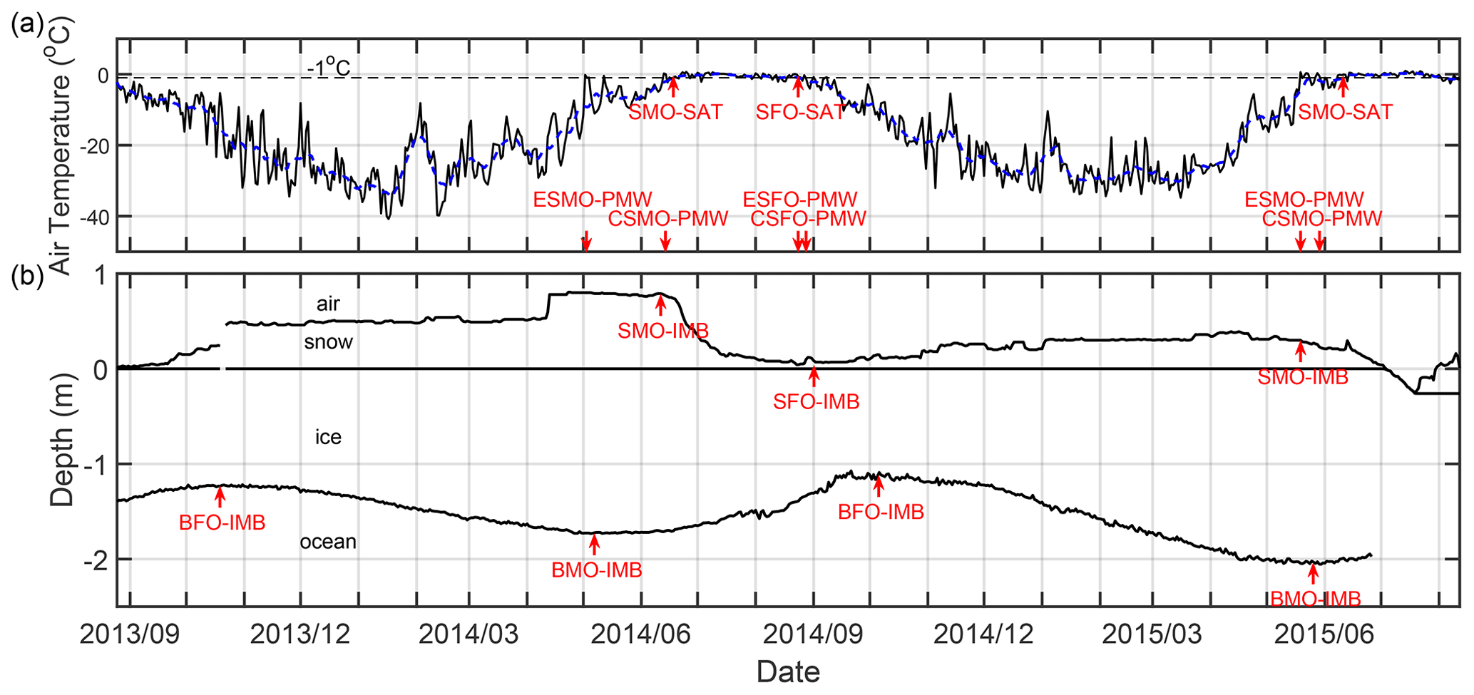
Figure 2 Detection of surface and basal melt and freeze onsets from IMB 2013F: (a) daily near-surface air temperature (black solid line) and its 14 d running-mean (blue dashed line); (b) snow depth and sea ice thickness, with the zero line denoting the initial snow–ice interface. The arrows indicate the melt and freeze onset dates estimated by the different methods.

3.1 Comparison of ice surface melt and freeze onsets from different methods

The four different SMOs and SFOs of 55 IMB trajectories from 2002 to 2018 are intercompared to each other. For the surface melt onset, SMO–SAT and CSMO–PMW matched best with the smallest deviation <2 d (Fig. 3), which means that the SAT threshold method captured the process of continuous ice surface melt quite reliably. The SMO–IMB was about 8–9 d earlier than the SMO–SAT and CSMO–PMW and 4 d later than the ESMO–PMW. Similar to IMB2013F (Fig. 2), the moderate deviations between SMO–IMB and SMO–SAT were mainly caused by spring storm events. Warm moisture carried by synoptic events from lower latitudes could lead to the SAT reaching the threshold temperature in a transitory period and promote surface snowmelt. However, such a temperature impulse could be missed by the 14 d running-mean filter. After the spring storms, the observed SAT dropped down and then increased and remained above the threshold temperature until the commencing of continuous surface melt.

For the surface freezing onset, both the SFO–IMB and SFO–SAT matched well with ESFO–PMW, with 2 d later and 3 d earlier than ESFO–PMW, respectively. The SFO–IMB occurred 8 d later than the SFO–SAT, which could also be attributed to the synoptic events and running-mean filter just as surface melt onset. Autumn storms brought about several temporary freeze–thaw cycles (i.e., snowfall and surface melting) before fully freezing. Thus, the transition date when the filtered SAT dropped below the threshold temperature was earlier than the date when the surface melt terminated. CSFO–PMW was always later than others, with an average delay of 13 d after SFO-SAT. These differences might be attributed to the spatial resolution, as the observations of ice mass balance and surface air temperature only represented a single point on an ice floe, while a PMW observation always represents a large area due to its footprint, which might include liquid water from melt ponds, leads, or open water.

In general, although the surface freeze–thaw cycles detected by the three methods show some moderate deviations, both surface melt and freeze onsets from the PMW and SAT methods generally match the results from the IMB observation quite well. In particular, the SMO–SAT and SFO–SAT reliably capture the “inner” melt season, the period between the CSMO–PMW and the ESFO–PMW (Markus et al., 2009). Here, the SMO–SAT and SFO–SAT are used as the general SMO and SFO for the purposes of comparing to the BMO/BFO and identification of the spatiotemporal variation, because the SMO–IMB and SFO–IMB were not available at some buoy sites.

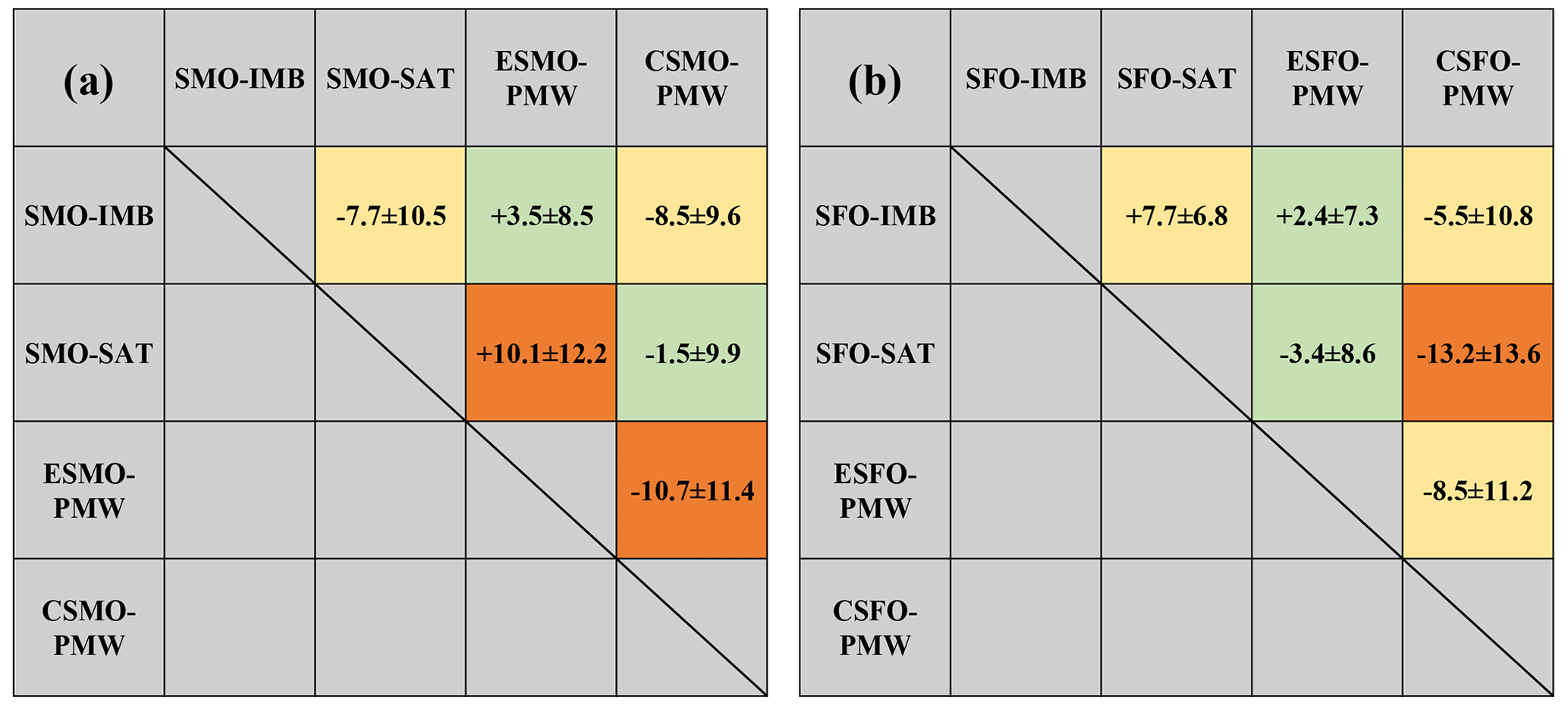
Figure 3 Differences (in days) of surface melt onset (SMO) (a) and surface freeze onset (SFO) (b) determined by the various methods (column minus row, “ + ” donates later and “−” donates earlier). The small (<5 d), moderate (5–10 d), and large (>10 d) deviations are indicated by the color of green, yellow, and orange, respectively.

3.2 Temporal and spatial variations of ice surface and basal melt and freeze onsets

The SMO, SFO, BMO, and BFO derived from 69 IMBs in the BG and CAO are presented in Fig. 4. The SMO ranged from mid-May to early July, with a mean on 12 June (±8 d) and a median on 14 June. The BMO ranged from late May to early July, with a mean on 5 June (±15 d) and a median on 3 June, approximately 7 d earlier than the SMO. The SFO ranged from early August to early September, with a mean on 20 August (±8 d) and a median on the same day. The BFO ranged from early October to late December, with a mean on 14 November (±21 d) and a median on 13 November. The average BFO lagged behind the corresponding SFO by almost 3 months. As a result, the average basal melt season was nearly 3 months longer than at the surface and was dominated by a later onset of basal ice growth.

The spatial variations in surface and bottom melt and freeze onsets were also remarkable under a certain variation of atmospheric and oceanographic conditions (Fig. 4). The overall spatial patterns revealed a shift in the surface and basal melt onsets to earlier dates, while the freeze onsets shift to later dates with a decrease in latitude, as one would expect. Sea ice generally melts earlier and freezes later in the BG compared to the CAO. The trends of the SMO and BMO against latitude were 0.6 ± 0.2 d per degree (p<0.001) and 2.0 ± 0.2 d per degree (p<0.001), respectively (Fig. 4e). In the BG, the average BMO (23 May) occurred approximately 17 d earlier than the SMO (9 June) for sea ice with a thickness of 2.36 ± 0.76 m. In the CAO, the BMO and SMO usually occurred almost at the same time (17 June vs 15 June) for sea ice with a thickness of 2.23 ± 0.47 m. The trend of the SFO against the latitude was −1.0 ± 0.3 d per degree (p<0.001), while the BFO exhibited a considerable amount of scatter with increasing latitude (Fig. 4e). The relevant mechanisms will be discussed later.

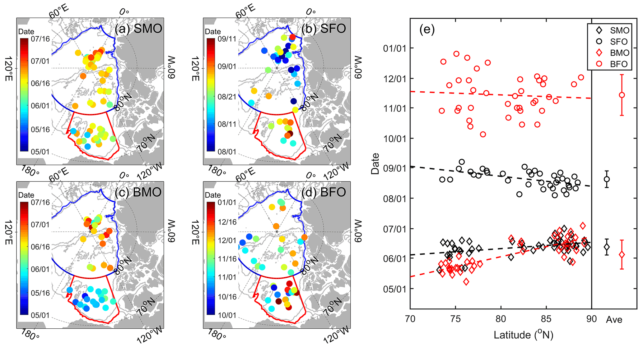
Figure 4 Timing of ice surface and bottom melt and freeze onsets of all sites: (a) SMO, (b) SFO, (c) BMO, and (d) BFO. The color codes (note the different scales for different panels) indicate the respective dates. Grey contours denote the 300 and 2000 m isobaths. (e) Variations in dates of melt and freeze onset as a function of the latitude.

3.3 Surface radiation budget during the transition between ice surface melting and freezing

Here, we extract the topmost snow temperatures from IMB temperature profiles to determine the thermodynamic state of the snow during the transition period from freezing to melting. Since the vertical resolution of the temperature profiles is only 0.1 m, the data of 33 IMBs with snow depths larger than 0.1 m are used. The topmost snow temperatures were averaged over 10 d before and after melt onset for each IMB. The average topmost snow temperature increased from −1.6 ± 1.2 ^∘C for the 10 d before the SMO to 0.1 ± 0.5 ^∘C for the 10 d after the SMO. Thus, the increase in the topmost snow temperature crossing the melting point can be considered one of the preconditions of the SMO.

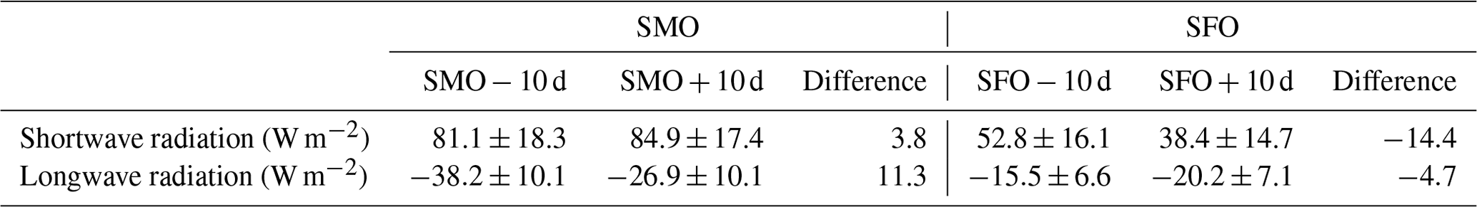
Similarly, using ERA5 reanalysis data, we evaluate the average net shortwave and net longwave radiation fluxes over a period of 10 d before and after the surface melt and freeze onsets for all available IMBs, with a positive value denoting a downwelling heat flux. The results are shown in Table 2. The average net shortwave radiation was 81.1 ± 18.3 and 84.9 ± 17.4 W m⁻² for the 10 d before and after the SMO, respectively, which amounts to an increase of 3.8 W m⁻². The corresponding average net longwave radiation was −38.2 ± 10.1 and −26.9 ± 10.1 W m⁻² for the 10 d before and after the SMO, which amounts to an increase of 11.3 W m⁻² (or the net loss decreased). The upward longwave radiation is calculated following the Stefan–Boltzmann law using top snow temperature, showing an increase of 7.8 W m⁻². Thus, the increase of downward longwave radiation is estimated to be as high as 19.1 W m⁻². These results are in line with previous findings stating that the ice surface melt onset in the Arctic is primarily triggered by an increase of downward longwave radiation (Maksimovich and Vihma, 2012; Persson, 2012). Warm and moist air masses carried northwards from lower latitudes by distinct synoptic events would increase the downwelling longwave radiation as well as the net longwave radiation, while the net shortwave radiation would not be altered too much due to the high snow albedo at the onset of surface melt (Persson, 2012). For the surface freeze onset, the average net shortwave radiation was 52.8 ± 16.1 and 38.4 ± 14.7 W m⁻² for the 10 d before and after the SFO, respectively, which amounts to a decrease of −14.4 W m⁻². Similarly, the average net longwave radiation was −15.5 ± 6.6 and –20.2 ± 7.1 W m⁻² for the 10 d before and after the SFO, which amounts to a decrease of −4.7 W m⁻². These contrasting results to the melt onset conditions are expected, as the SFO is primarily controlled by the decline of net shortwave radiation with the approach of the polar night.

Table 2 Average surface net radiation changes during the transition from surface melting to freezing, calculated from ERA5 reanalysis data.

3.4 Heat balance at the ice–ocean interface during basal melt and growth onsets

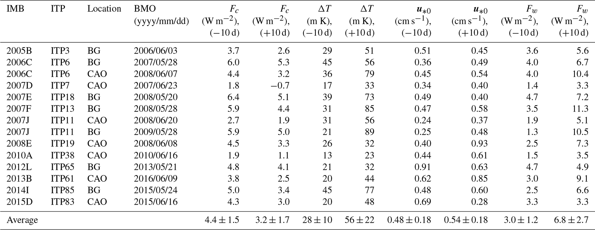
We compare ΔT, u_*0, F_w, and F_c during the 10 d before (−10 d) and after (+10 d) our calculated BMO using data from 12 pairs of co-located IMBs and ITPs (Table 3). The average ΔT (−10 d) ranged from 13 to 45 mK, with a mean of 28 ± 10 mK. This was warmer than the typical winter mixed-layer temperature (within a few mK of the freezing point, Shaw et al., 2009). The average ΔT (+10 d) was almost twice as large as ΔT (−10 d), with a mean of 56 ± 22 mK. u_*0 did not show any significant changes. Therefore, the change of ocean heat flux into the ice should be governed by the thermodynamic processes rather than the dynamics. The estimated F_w increased from 3.0 ± 1.2 to 6.8 ± 2.7 W m⁻², which was substantially larger than the typical winter value of about 1.0 ± 2.9 W m⁻² in the Canada Basin (Cole et al., 2014) and 2.1 ± 2.3 W m⁻² in the Eurasian Basin (Peterson et al., 2017). During the cold winter, the typical sea ice temperature profile is almost linear (Lei et al., 2014). As the summer approaches, the upper ice column warms faster than its lower portion, leading to a “C-shape” vertical temperature profile with a gradually reduced temperature gradient at the ice base (Lei et al., 2014). Correspondingly, the upward average conductive heat flux at the ice bottom decreased from 4.4 ± 1.5 to 3.2 ± 1.7 W m⁻². The key influence on the BMO is when F_w becomes greater than F_c. Therefore, once the upward oceanic heat flux surpasses the upward conductive heat flux at the ice bottom, ice basal melt commences.

The surface ocean typically warms earlier in the BG compared to the CAO due to the larger amount of incoming solar radiation in lower latitudes. At the same time, both remote sensing and models revealed that sea ice in the BG shows higher divergence and larger water fraction compared to the CAO (Wernecke and Kaleschke, 2015; Wang et al., 2016), as well as a higher fraction of thin ice (Petty et al., 2020). Consequently, the upper ocean in the BG absorbs more solar radiation compared to the CAO (e.g., Perovich et al., 2011). This may at least partly explain why in the BG the BMO occurred much earlier than the SMO, while it occurred almost at the same time in the CAO.

Table 3 Summary of the changes of oceanic heat flux from the observations of ITP on BMO.

We further investigate the mechanism relevant to the time lag between the BFO and SFO from the perspectives of both the sea ice itself and the underlying ocean. According to the heat balance at the ice–ocean interface, sea ice basal growth begins when the heat transported away from the ice bottom due to the upward conductive heat flux is greater than the heat transfer into the ice by the oceanic heat flux. IMB 2007J and ITP11 were co-located on the same ice floe, which drifted southward in the east of Canada Basin during the period between the SFO and BFO (Fig. 5a), giving a simultaneous thermodynamic observation of the ice and the underlying ocean. As shown in the IMB 2007J data (Fig. 5b), the relatively warm sea ice column in summer began to cool downward from the surface to the bottom as a result of the decreasing SAT. Correspondingly, the conductive heat flux in the sea ice basal layer gradually shifted from downward to upward as the freezing front gradually moved downward through the ice column. At the same time, data from the co-located ITP11 revealed that the remaining heat stored in the mixed layer is transported upwards to continue to melt the ice base or delay ice growth. Subsequently, the mixed-layer temperature decreased gradually to the freezing point (Fig. 5c), which took ∼ 63 d after the SFO. During this period, the ice floe drifted southward into a region with much warmer subsurface water just beneath the mixed layer, i.e., a stronger near-surface temperature maximum (NSTM, Fig. 5d). As a result, although the oceanic mixed-layer temperature dropped to the freezing point in late October 2008, basal freezing did not commence until mid-November 2008, when the upward conductive heat flux increased to >10 W m⁻². The upward heat transport was balanced by the subsurface oceanic heat release from the NSTM (Fig. 5c), which delayed basal ice growth by approximately 21 d. The heat stored in the NSTM was held in place by the strong stratification of the summer halocline and was finally released by a halocline erosion induced by shear-driven entrainment (Toole et al., 2010; Jackson et al., 2012; Lin and Zhao, 2019). In summary, the slow propagation of the freezing front from the ice surface to the bottom, combined with the oceanic heat release from the mixed layer and subsurface ocean, jointly resulted in the time of BFO approximately 3 months later than SFO.

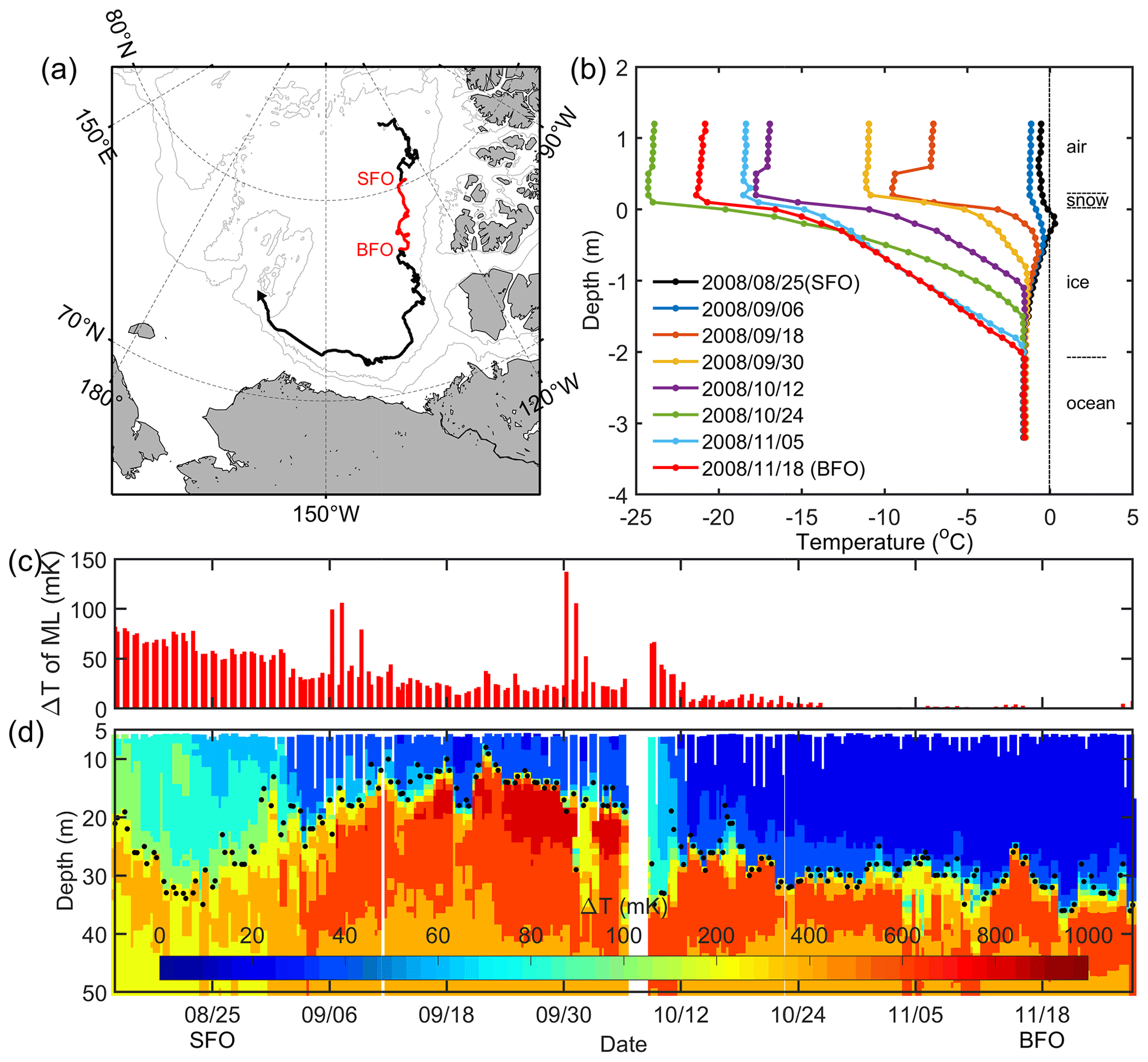
Figure 5 (a) Drift trajectory of co-located IMB 2007J and ITP 11; (b) IMB 2007 temperature profiles from SFO (black line) to BFO (red line); (c) mixed-layer temperature deviation from the in situ freezing point; (d) ITP 11 profiles of temperature deviation from the in situ freezing point. Black dots indicate the mixed-layer depth where the potential density relative to 0 dbar first exceed the shallowest sampled density by 0.01 kg m⁻³. The white vertical bar in early October 2008 indicates a data gap.

3.5 Impact of air temperature and ice thickness on basal ice growth onset

As explained above, the cooling of the sea ice is one of the preconditions of basal ice growth. Thus, we quantitatively analyze the role of sea ice cooling on the BFO. In order to minimize the impact of spatial variations, we use the time delay between the BFO and SFO instead. Near-surface air temperature, snow depth, ice thickness, and ice internal structure (brine volume fraction) are suggested as the crucial factors controlling the cooling efficiency of the sea ice column, or worded differently, the propagation efficiency of the freezing front from the sea ice surface to the bottom (which is the prerequisite for the BFO). The influence of the ice internal structure cannot be assessed using IMB data; thus we do not consider its influence here. The lower SAT accelerates the sea ice cooling, while a thicker snow cover as a thermal insulator plays the opposite role due to its low thermal conductivity (Ledley, 1991). Thereby, an ice cooling index (ICI) is introduced here as

$$\begin{array}{}\text{(4)}& \mathrm{ICI}=H_{\mathrm{is}}/\mathrm{FDD},\end{array}$$

where

$$\begin{array}{}\text{(5)}& H_{\mathrm{is}}=H_{\mathrm{i}}+k_{\mathrm{i}}/k_{\mathrm{s}}\cdot H_{\mathrm{s}}.\end{array}$$

H_is, H_i, and H_s are the equivalent ice thickness, ice thickness, and snow depth, respectively. k_i (2 W m⁻¹ K⁻¹) and k_s (∼ 0.3 W m⁻¹ K⁻¹) are the thermal conductivities of ice (Yen et al., 1991) and snow (Sturm et al., 2002), respectively. FDD is the amount of seasonal cumulative freezing degree days, which is defined as the time-integrated daily air temperature below the seawater freezing point (−1.8 ^∘C), with the SFO as the zero reference. H_i is defined as the mean ice thickness between the SFO and BFO because the ice thickness at the BFO can be thinner by as much as 0.63 m compared to that at the SFO (IMB 2011K). The IMB data showed that snow accumulation usually occurred just after the SFO, with snow mostly accumulating in the early freezing season and maintaining a steady state until the surface melt occurred. Thus, H_s is defined as the mean snow depth between the SFO and BFO. The time delay between the BFO and SFO ranged from 38 to 115 d, with a mean of 82 ± 26 d. For consistency and comparability, we defined the same period for FDD integration starting from SFO. The most significant relationship between the ICI and the time lag between the BFO and SFO was found if the integration time is chosen as 45 d, with R=0.81, p<0.01 (Table 4, Fig. 6).

Generally, the lower surface air temperature, thinner sea ice, and thinner snow cover are related to the earlier basal ice growth and vice versa, suggesting the time lag between the BFO and SFO can be significantly attributed to the ice column cooling efficiency. Without considering the SAT, H_is also has a significant relationship with the time lag (R=0.79, p<0.05) because the SAT does not show significant differences between the buoys. These results imply a negative feedback; i.e., thinner snow and ice favor earlier basal freeze-up in the following winter. Since sea ice thickness and snow depth of each IMB vary in a wide range, that is the most likely explanation why the BFO exhibits a much larger variability.

Table 4 Ice cooling index (ICI) and time lag between BFO and SFO.

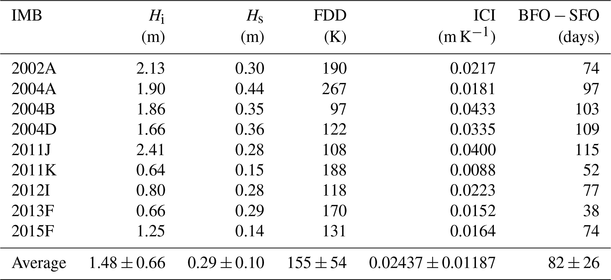
Figure 6 The relation between ice cooling index (ICI) and the time lag between the onset of surface freeze and basal ice growth. The color map represents the equivalent ice thickness. The inset map shows the average position of each IMB during the period between SFO and BFO. The red asterisk denotes the North Pole.

3.6 Relationship between the melt and freeze season length and the amount of ice melt/freezing

Sea ice surface melt includes surface snowmelt and surface ice melt. The equivalent surface melt (ESM) is defined as

$$\begin{array}{}\text{(6)}& \mathrm{ESM}=({\mathit{\rho }}_{\mathrm{s}}/{\mathit{\rho }}_i{)}_{\mathrm{s}}\mathrm{\Delta }{H}_{\mathrm{s}}+\mathrm{\Delta }{H}_{\mathrm{i}},\end{array}$$

where ΔH_s and ΔH_i are surface snow and ice melt, respectively; ρ_s=300 kg m⁻³ is the snow density; and ρ_i=900 kg m⁻³ is the ice density (Perovich et al., 2014). Here, surface snow and ice melt are inferred from a combination of surface acoustic sounder observations and the distinct difference of temperature gradients in air, snow, and ice. In agreement with a previous study by Lindsay (1998), the total surface melt was correlated with the length of the surface melt season (R=0.48, p<0.01) and increasing by 0.07 m with a lengthening of the surface melt season by 10 d (Fig. 7a). Surface melt is determined by the surface energy balance, which is influenced by surface albedo, radiation, and turbulent fluxes, as well as wind erosion and evaporation (Persson, 2012). Based on SHEBA data, Perovich et al. (2003) found that a thinner snow cover was related to an earlier surface ice melt but that the initial snow depth seems to have no impact on the total surface melt. Here, based on the IMB observations, the initial snow depth at the surface melt onset exhibits a correlation with the total surface melt ($R=-\mathrm{0.52}$, p<0.01; Fig. 7b), which is a manifestation of the well-known albedo feedback. The reason for the above differences may be that the ice mass balance observations were carried out on a variety of different ice surface topographies during SHEBA, which were likely susceptible to surface meltwater redistribution and horizontal heat advection, while the IMB deployment locations are usually biased towards level ice.

As shown in Fig. 7c, no direct relationship was identified between the total basal melt and the basal melt season length. Larger basal melt was always accompanied by a longer basal melt season, but the opposite was not always true. The ice concentration around the IMB can affect the amount of ice basal melt by adjusting the shortwave radiation budget of the ice–ocean system. For comparison, the lengths of the basal melt season of IMBs 2004A, 2005B, and 2006C were 170, 174, and 172 d, respectively. However, the mean June–September ice concentrations along the drifting trajectories of IMB 2004A, 2005B, and 2006C were distinctly different, with values of 99 %, 89 %, and 71 %, respectively. As a result, the basal melt at IMB 2006C (2.14 m) was nearly 3 times larger than at IMB 2005B (0.77 m) and 10 times larger than at IMB 2004A (0.22 m) because the lower ice concentration causes more shortwave radiation to be absorbed by the upper ocean. This suggests that the total basal melt does not significantly correlate with the initial ice thickness when basal melt begins (Fig. 7d) but is more likely related to the amount of solar heat input into the upper ocean in summer (Stanton et al., 2012). If we exclude the individual BMOs impacted by early spring storms, such as the BMO of IMB 2013F in 2014, the BMO was significantly correlated with the total basal melt (R=0.82, p<0.01); i.e., earlier BMO always leads to more basal melt (not shown).

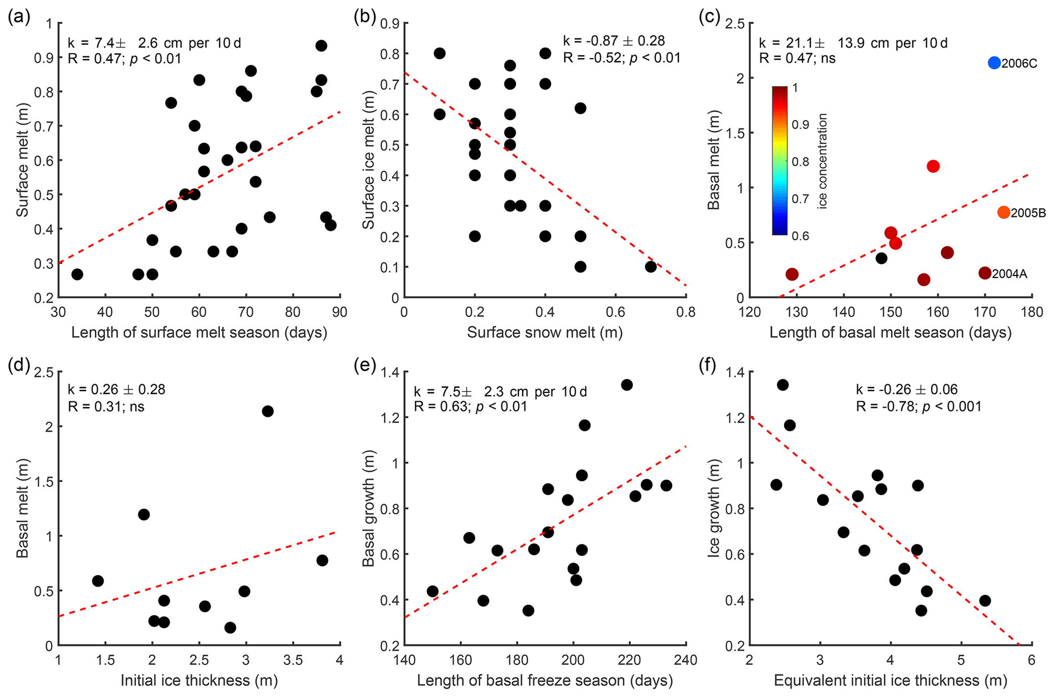
Figure 7 Relationships between (a) length of surface melt season and total surface melt, (b) surface snowmelt and surface ice melt, (c) length of basal melt season and total basal melt, (d) initial ice thickness and basal melt, (e) length of basal freeze season and total basal growth, and (f) equivalent initial ice thickness and total ice growth.

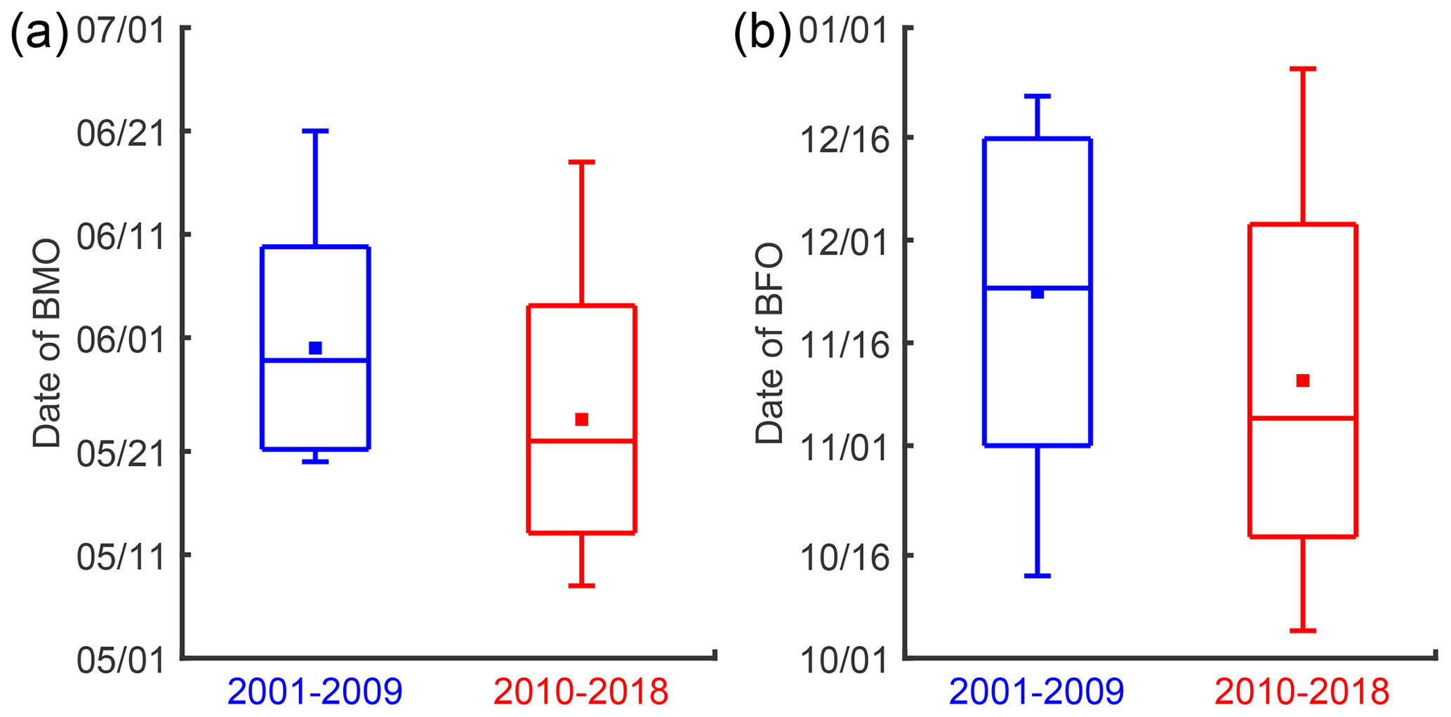
Figure 8 Decadal changes in BMO (a) and BFO (b) obtained from Lagrangian IMB observations in the Beaufort Gyre. The solid square is the mean, the horizontal line is the median, the box represents ±1 SD (standard deviation), and the whiskers are the maximum and minimum values.

It is also notable that the total basal growth shows a significant correlation (R=0.63, p<0.01) with the length of the basal freeze season (Fig. 7e). As investigated above with IMB observations, basal growth of thinner sea ice started earlier compared to thicker ice. In combination with the negative conductive feedback (i.e., thinner ice grows faster than thicker ice), thinner ice generally experienced a longer freezing season and a larger ice growth. Considering the thermal insulation effect of the snow cover, the initial equivalent ice thickness H_is (defined above) was used to identify the link between the initial ice thickness and the total ice growth. As shown in Fig. 7f, the total sea ice growth during the entire freezing season increased by 0.26 m with the initial H_is decreasing by 1 m. For all IMBs that experienced the complete melting or freezing seasons, the average ice melt was 0.56 m at the surface and 0.65 m at the ice bottom, while the average ice growth was 0.74 m. Thus, the average annual ice thickness budget derived from all IMB observations during 2000–2018 amounts to −0.47 m, which clearly confirms the ongoing decline of the Arctic sea ice thickness. One remarkably similar result was for example presented by Petty et al. (2020), who used the February–March ice thickness retrieved from the satellite altimeter measurement of ICE-Sat (Ice, Cloud, ad land Elevation Satellite) to show a decrease of ∼ 0.37 m or ∼ 20 % thinning across an inner Arctic Ocean domain from 2008 to 2019. We infer that the growth of multiyear sea ice in winter is not sufficient to compensate for the melt in summer, even though the negative conductive feedback enhances the ice growth during the freezing season.

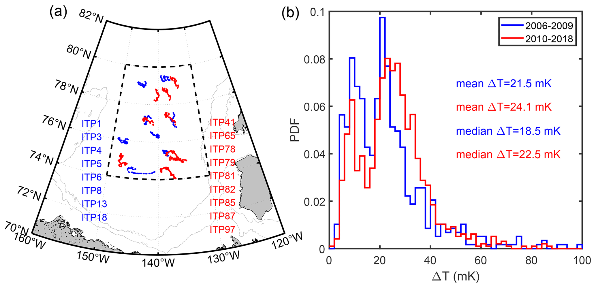
Figure 9 (a) ITP drift trajectories in the central Beaufort Gyre in May; (b) scaled histograms of the mixed-layer temperature departure from the local freezing point in the central BG in May with bin size of 2 mK. PDF: probability distribution function.

3.7 Decadal changes of basal melt and freeze season length in the Beaufort Gyre

As shown in Fig. 4c and d, the basal melt and freeze onsets derived from IMB observations revealed a large spatial variation, especially in the CAO. To minimize the impact of spatial variations, we estimate here the decadal changes in the BMO and BFO in the BG using a synthetic analysis (Fig. 8). All BMOs and BFOs detected from the IMB observations were equally divided into two 9-year periods. The average BMOs were on 31 May in 2001–2009 (9 cases) and 24 May in 2010–2018 (17 cases), respectively. Similar to the SMO, there is also a trend towards earlier BMO, which occurred approximately 7 d earlier in the recent 9 years compared to the previous 9 years. Although the trend was relatively weak, all available ITP observations in this period in the central BG indicate the average oceanic mixed-layer temperature departure from the local freezing point (ΔT) in May was 24.1 mK in the recent 9 years and 21.5 mK in the previous 9 years (Fig. 9), which can be partly explained by more frequent lead openings in early spring (e.g., Qu et al., 2021). The average BFO was on 15 November in 2010–2018 (15 cases), which was 8 d earlier than (23 November) in 2001–2009 (9 cases) and which is in line with thinner ice favoring an earlier onset of basal ice growth (1.30 m vs. 1.83 m).

Considering that the IMB observations were mainly obtained on multiyear ice and therefore do not necessarily catch the freezing and thawing of the seasonal sea ice, we also investigate the decadal changes of the melt and freeze onsets using ULS data from three moorings in the BG (moorings A, B, and D) to reveal potential biases in our previous analysis. Mooring C is excluded due to its relatively short observation period. Since our earlier results indicate that the BMO in the BG occurs approximately 17 d earlier than the SMO, it is reasonable to define the date of the annual total ice thickness maximum as determined from the ULS data as the BMO. Defining the date of the ULS annual total ice thickness minimum as the general BFO is more debatable, especially due to the simultaneous snow accumulation and basal melting. However, most of the IMB observations revealed that the snow depth was already relatively stable at the BFO around November–December. Thus, we consider it acceptable to define the FO obtained from the ULS data as the BFO.

The observed ice thickness from three moorings (A: 75^∘ N, 150^∘ W; B: 78^∘ N, 150^∘ W; D: 74^∘ N, 140^∘ W) and calculated BMOs and BFOs during 2004–2018 are shown in Figs. 10 and 11. For comparison with results from the IMB observations presented above, all ULS BMOs and BFOs were divided into the same two periods of 2004–2009 and 2010–2018. The results revealed that the BMO advanced in all three moorings, but the tendencies were insignificant at the 95 % confidence level. The average BMO in mooring A was nearly the same in the two periods (23 May vs. 22 May). At the same time, the average BMO in mooring B has been shifting to an earlier date from 10 June in 2004–2009 to 30 May in 2010–2018. The average BMO in mooring D also occurred earlier by 5 d from 1 June in 2007–2009 to 27 May in 2010–2018. The advance of the BMO obtained from the ULS data is consistent with the results obtained from the IMBs. However, the BFOs obtained from IMBs and ULSs revealed a different change trend. The BFO in mooring A was delayed by 15 d from 25 September in 2004–2009 to 10 October in 2010–2017. In contrast, in the northernmost mooring B, which showed a later BFO in 2004 and 2006, the BFO advanced by 8 d from 8 October in 2004–2008 to 30 September in 2011–2017. In fact, since 2008, the BFO of mooring B also exhibited a delay. The BFO in mooring D was nearly the same between the two periods (29 September vs. 30 September). Moorings A and D were located in the southern part of the BG, where the summer has been typically ice-free almost every year since 2007, except for 2013. When the sea ice melted completely, the BFO was almost the same as the SFO. Thus, the accelerated loss of sea ice and the frequent occurrence of ice-free summers in the BG may contribute to a later freeze-up due to more solar heating of the ocean.

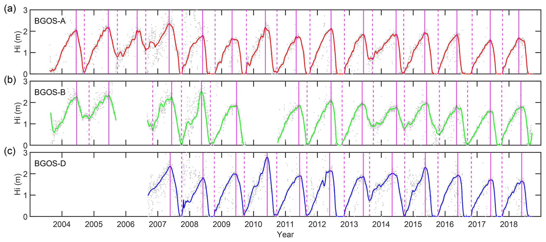
Figure 10 Time series of filtered ice thickness observed by ULS in the BG (BGOS-A: red; BGOS-B: green; BGOS-D: blue); grey dots denote the daily ice thickness, with magenta solid and dashed lines indicating the BMO and BFO, respectively.

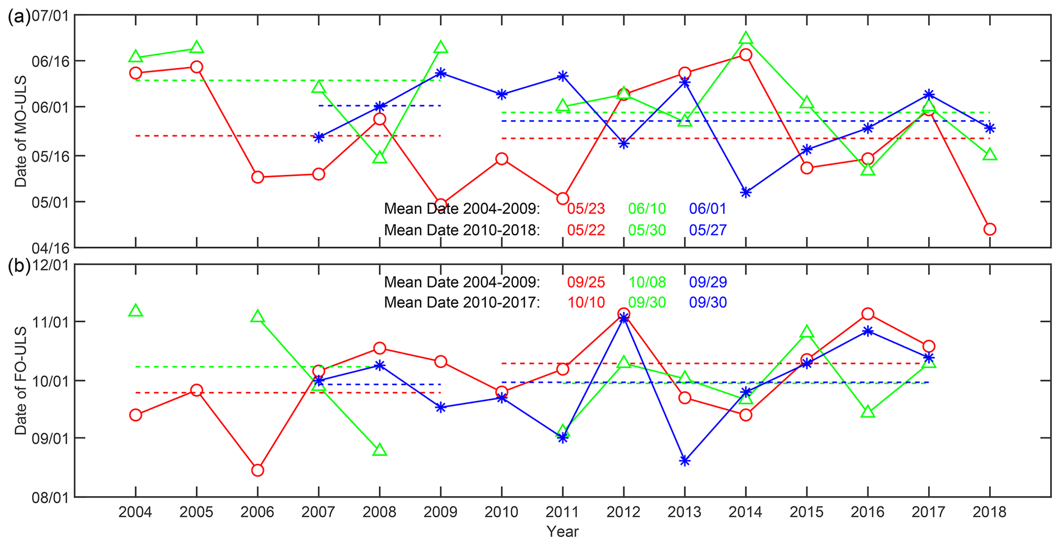
Figure 11 Interannual variations in (a) MO-ULS and (b) FO-ULS (BGOS-A: red; BGOS-B: green; BGOS-D: blue); dashed lines denote the average of each period of 2004–2009 and 2010–2017.

4 Conclusions

In this study, we determined the timings of sea ice annual freeze–thaw cycles in the Beaufort Gyre and central Arctic Ocean using a multisource data approach. Our main focus was on the detailed analysis of observations obtained by a large number of ice mass balance buoys (IMBs), which we used as a reference to compare our results calculated from satellite passive microwave (PMW) data. Since the IMB dataset may be potentially biased towards thicker and older sea ice, we additionally supplemented this analysis with observations from upward-looking sonars (ULSs) on moorings.

Based on these three very different datasets, we calculate and intercompare four pairs of surface melt and freeze onsets and two pairs of basal melt and freeze onsets that we determined using distinct automated algorithms. Our results reveal that the PMW and SAT threshold methods can reliably capture the surface melt and freeze cycle when compared with reference IMB surface mass balance observations. The average BMOs were comparable in the central Arctic Ocean and approximately 17 d earlier than SMOs in the Beaufort Gyre. The average BFOs were lagging behind almost 3 months compared to the SFOs for the pan Arctic Ocean.

During the transition of the SMO, the topmost snow temperature increased to above melting, indicating the start of surface melt. Reanalysis data indicated that the SMO was primarily driven by longwave radiation rather than shortwave radiation. In contrast, the SFO is driven by seasonal decline of shortwave radiation. Synchronous ice and underlying ocean observations confirmed that the ice bottom melt began when oceanic heat flux surpassed the upward conductive heat flux at the sea ice bottom. The ice basal freeze-up delay relative to the surface can be attributed to the regulation of heat capacity of sea ice itself and the oceanic heat release from ocean mixed layer and subsurface layer. The ice cooling index determined by the near-surface air temperature, snow depth, and ice thickness shows a significant correlation with the temporal delay between BFO and SFO, with lower surface air temperature, thinner sea ice, and thinner snow cover favoring earlier onset of basal ice growth and vice versa.

In the Beaufort Gyre, both Lagrangian IMB observations and Eulerian ULS observations exhibit a trend towards earlier basal melt onset, which can be attributed to the earlier warming of the surface ocean. In contrast, there is a trend towards earlier onset of basal ice growth evident from the IMB observations, which is associated with the reduction of ice thickness of the multiyear ice. At the same time, we determined a trend towards delayed onset of basal ice growth in the ULS observations because of the frequent occurrence of ice-free summers in the southern Beaufort Gyre region in recent years.

Note that, some limitation of our results should be considered. First, IMBs only collected one-dimension point measurements of mass balance and are representative of the special ice floe where they are deployed. As a result, the melt and freeze onsets of other ice categories such as ponded ice and ridged ice are out of our scope. Second, interior ice melt, surface pond, and false bottoms, as well as the unfrozen cavities within the rubble of ridges, greatly affected the energy budget consequently the basal melt and freeze (Shestov et al., 2018; Provost et al., 2019; Smith et al., 2022). But the effect for these different conditions could have was not considered in our study. Third, the majority of IMBs were deployed on multiyear undeformed ice (Planck et al., 2020), so the basal melt and freeze onsets of seasonal ice are underrepresented. Compared to multiyear ice, seasonal ice has higher bulk brine, resulting in a smaller specific heat capacity and latent heat of fusion (Tucker et al., 1987; Wang et al., 2020), as well as a higher permeability during the summer (Lei et al., 2022), thus affecting the sea ice basal melt and freeze processes. Finally, due to the limited vertical observation range of ocean profile automatic observation instruments, some special processes near the ice bottom, such as supercooling and false bottoms, were not characterized well.

Therefore, more intensive and elaborative ice mass balance observations of diverse ice types by IMB observations and other methods and simultaneous upper-ocean water properties observations in the future will vastly improve our capability to fully understand the ice–ocean system and the mass balance of sea ice in a changing Arctic.