Thermal regime of the Grigoriev ice cap and the Sary-Tor glacier in the inner Tien Shan, Kyrgyzstan

The thermal regime of glaciers and ice caps represents the internal distribution of ice temperatures. An accurate knowledge of the thermal regime of glaciers and ice caps is important to understand their dynamics and response to climate change and to model their evolution. Although the assumption is that most ice masses in the Tien Shan are polythermal, this has not been examined in appropriate detail so far. In this research, we investigate the thermal regime of the Grigoriev ice cap and the Sary-Tor glacier, both located in the inner Tien Shan in Kyrgyzstan, using a 3D higher-order thermomechanical ice flow model. Input data and boundary conditions are inferred from a surface energy mass balance model, a historical air temperature and precipitation series, ice thickness measurements and reconstructions, and digital elevation models. Calibration and validation of the englacial temperatures are performed using historical borehole measurements on the Grigoriev ice cap and radar measurements for the Sary-Tor glacier. The results of this study reveal a polythermal structure of the Sary-Tor glacier and a cold structure of the Grigoriev ice cap. The difference is related to the larger amount of snow (insulation) and refreezing meltwater (release of latent heat) for the Sary-Tor glacier, resulting in higher surface layer temperature, especially in the accumulation area, which is subsequently advected downstream. Further, ice velocities are much lower for the Grigoriev ice cap, with consequent lower horizontal advection rates. A detailed analysis concerning the influence of temperature and precipitation changes at the surface reveals that the thermal structure of both ice bodies is not constant over time, with recent climate change causing increasing ice temperatures in higher areas. The selected ice masses are representative examples of the (inner) Tien Shan glaciers and ice caps. Therefore, our findings and the calibrated parameters can be generalised, allowing improved understanding of the dynamics and future evolution of other glaciers and ice caps in the region.

1 Introduction

Global warming is causing an unprecedented loss of glaciers that is expected to continue and have far-reaching consequences for worldwide water availability, even without further temperature increase (Zemp et al., 2019). High Mountain Asia (HMA), comprising several glacierised mountain ranges such as the Himalayas, Karakoram, Pamir, and Tien Shan, contains the highest concentration of glaciers globally (Bhattacharya et al., 2021). However, glaciers in HMA also involve one of the largest uncertainties in current and future ice volume assessments (Farinotti et al., 2019). The englacial temperatures are an important characteristic influencing the dynamics and behaviour of glacier ice (Gilbert et al., 2020). The thermal regime of an ice mass, describing the englacial temperature structure, is universally categorised into three types: cold (containing cold ice, possibly with a thin layer of temperate ice at the base), temperate (containing only temperate ice; i.e. the ice temperature reaches the pressure melting point everywhere), and polythermal (containing cold and temperate ice) (Blatter and Hutter, 1991). Accurate knowledge of the ice temperatures is important because ice deformation depends on the ice temperature, meltwater routing is affected by ice temperature, and the basal temperature determines whether the ice mass can slide over its base (Blatter and Hutter, 1991; Hambrey and Glasser, 2012; Gilbert et al., 2020). Hence, precise knowledge of the thermal regime of ice bodies is needed to understand and accurately model their response to climate change (Gilbert et al., 2020).

The focus of this study is on the Tien Shan, where ice masses are assumed to be mostly cold and polythermal (Vilesov, 1961; Maohuan et al., 1982; Echelmeyer and Zhongxiang, 1987; Vasilenko et al., 1988; Petrakov et al., 2014; Nosenko et al., 2016). Previous studies demonstrated a polythermal structure using borehole measurements for the Ürümqi glacier (Cai et al., 1988) and the Davydov glacier (Vasilenko et al., 1988). Using ground-penetrating radar (GPR) measurements, other studies revealed the presence of cold and temperate layers on the Sary-Tor glacier (Petrakov et al., 2014); the Tuyuksu glacier (Nosenko et al., 2016); and the Abramov glacier, located in the nearby Pamir Alay (Kislov et al., 1977). According to measurements on the Abramov glacier, the Ürümqi glacier, and the Tuyuksu glacier, temperate ice was present near the surface of the lower part of the accumulation area (Kronenberg et al., 2021) and over a large area at the base (Nosenko et al., 2016). The latter was corroborated by larger summer velocities compared to winter velocities, indicating that basal sliding was occurring on the Ürümqi glacier in the Chinese Tien Shan (Maohuan et al., 1989; Maohuan, 1992). Parts of the inner Tien Shan glaciers have also been categorised as surge-type glaciers (Mukherjee et al., 2017; Bhattacharya et al., 2021). The surge behaviour has been interpreted by the polythermal structure of the ice masses with a cold mantle at the front restraining ice movement. After a long period with ice thickening and steepening in the upper reaches, the cold mantle at the front is supposed to be destructed, followed by an advance over a short period of time (Nosenko et al., 2016; Mukherjee et al., 2017). Few (11) of such glaciers were identified in the Ak-Shyirak massive, including the northern Bordu glacier and the Davydov glacier, located in the valleys next to the Sary-Tor glacier (Bondarev, 1961; Mukherjee et al., 2017).

The temperate ice in the lowest part of the accumulation area has typically been explained by an infiltration congelation/recrystallisation zone, characteristic for the continental climate in which the ice masses are located (Shumskiy, 1955; Vilesov, 1961; Maohuan et al., 1982; Maohuan, 1990; Osmonov et al., 2013; Petrakov et al., 2014). In the lowest part of the accumulation area, the ice and snow surfaces are warmed significantly by the infiltration and refreezing of meltwater releasing latent heat (Shumskiy, 1955; Lüthi et al., 2015). Such a temperate area in the infiltration zone has also been observed at other sub-polar glaciers such as Storglaciären in Sweden (Hooke et al., 1983). But, in addition to the influence of refreezing meltwater, other processes play a role in the warming and cooling of surface layers, such as a seasonal snow cover that shields the underlying ice from the extremely cold air temperatures during winter (Hooke et al., 1983) or the ablation of ice, which removes the warm or cold ice from above (Blatter, 1987; Wohlleben et al., 2009).

Here, we investigate the thermal regime of the Grigoriev ice cap and the Sary-Tor glacier, both located in the inner Tien Shan, Kyrgyzstan (central Asia), using a three-dimensional (3D) higher-order (HO) thermomechanical ice flow model coupled to a simplified 2D surface energy mass balance model. The selected ice flow model has been successfully applied at different scales, ranging from a medium-sized mountain glacier in the Alps (Zekollari et al., 2013, 2014; Zekollari and Huybrechts, 2015), and a medium-sized ice cap in Greenland (Zekollari et al., 2017) to the entire Greenland ice sheet (Fürst et al., 2013, 2015). To date, most of the 3D glacier and ice cap model studies have been performed assuming an isothermal state of the ice mass (e.g. Jouvet et al., 2011; Zekollari et al., 2014). Only a few studies have been performed by applying a 3D thermomechanical ice flow model including variations in englacial temperatures for glaciers (Zwinger et al., 2007; Zwinger and Moore, 2009; Zhao et al., 2014; Rowan et al., 2015; Li et al., 2017; Gilbert et al., 2017, 2020) and ice caps (Flowers et al., 2007; Schäfer et al., 2015; Zekollari et al., 2017).

In this study, we perform different experiments under constant 1960–1990 average climatic conditions. Afterwards, multiple sensitivity experiments are carried out to determine the influence of parameter choice, to assess the uncertainty in the results, and to determine the impact of changing climatic conditions at the surface on the thermal structure of both ice bodies. Several datasets are used for calibration and validation. For the Grigoriev ice cap, ice thickness measurements were performed in August 2021 with a GPR system and used for a glacier-wide ice thickness reconstruction. Ice temperatures derived from ice cores made in 1962 (Dikikh, 1965), 1990 (Thompson et al., 1993), 2001 (Arkhipov et al., 2004), and 2007 (Takeuchi et al., 2014), distributed over the ice cap, are used as calibration and validation for the thermal structure. Historical surface mass balance measurements from different periods are used to calibrate the mass balance model (Dyurgerov, 2002; Arkhipov et al., 2004; Fujita et al., 2011). Concerning the Sary-Tor glacier, observed and reconstructed ice thicknesses from 2013 are adopted (Petrakov et al., 2014), recent mass balance measurements are used, and radargrams displaying cold and temperate ice are considered for the validation of the thermal structure.

2 Study area

2.1 The Grigoriev ice cap and the Sary-Tor glacier

The Grigoriev ice cap (∼ 7 km²) (also called flat-top glacier) is located at the southern slopes of the Terskey Ala-Too mountain range in the inner Tien Shan in Kyrgyzstan (central Asia) (Fig. 1). The ice cap is located between the valleys of the Chontor glacier (to the west) and the Popova glacier (to the east). The top of the Grigoriev ice cap is a flat snow field at an elevation between 4500 and 4600 m a.s.l. In contrast to a typical valley glacier, the ice of the Grigoriev ice cap flows in multiple directions, ending at steeper glacier fronts and at multiple smaller outlet glaciers (Fig. 1). The northern boundary of the Grigoriev ice cap is also characterised by ice cliffs where mass is lost due to dry calving. The Grigoriev ice cap has been subject to numerous glaciological investigations such as mass balance measurements (Mikhalenko, 1989; Fujita et al., 2011) and ice core drilling (Dikikh, 1965; Thompson et al., 1993; Arkhipov et al., 2004; Takeuchi et al., 2014, 2019). In August 2021, we measured the ice thickness of the Grigoriev ice cap with a GPR system, following the approach of Van Tricht et al. (2021a).

The Sary-Tor glacier is a small valley glacier (∼ 2 km²), located in the north-western part of the Ak-Shyirak massif, roughly 30 km to the south-east of the Grigoriev ice cap (Fig. 1). Its ice thickness was measured in 2013 with a GPR system, showing a maximum ice thickness of almost 160 m (Petrakov et al., 2014). Annual mass balance measurements on this glacier have been performed since 2014, and these are deposited in the World Glacier Monitoring Surface (WGMS) database. Because debris cover is almost entirely absent on the Sary-Tor glacier, the glacier changes are assumed to directly reflect the changing climate in the inner Tien Shan (Petrakov et al., 2014). The Sary-Tor glacier has therefore typically been used as a reference glacier for the surrounding area, especially for the Ak-Shyirak massive (Mikhalenko, 1993). Van Tricht et al. (2021b) calibrated a surface energy mass balance model for the Sary-Tor glacier and reconstructed the historical mass balance between 1750 and 2020, showing a significant decrease in the mean specific mass balance, especially since the 1970s. Recently, the concession of the Kumtor gold mine, which is located north of the glacier (Fig. 1), was extended towards the valley of the Sary-Tor glacier, removing the terminal moraines of the Little Ice Age (LIA).

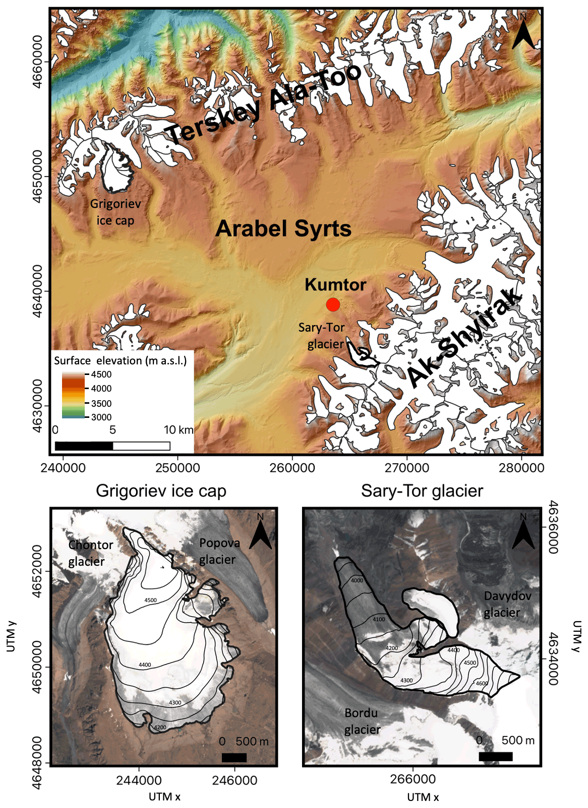
Figure 1 The Grigoriev ice cap and the Sary-Tor glacier located in their respective mountain range in the inner Tien Shan. All the glaciers of the Randolph Glacier Inventory version 6 (from 2002) are indicated in white colour on the upper map. The black outline of the glaciers in the lower maps represents the extent of the ice mass in August 2021. Glacier elevation contours are added for every 50 m. The location of the Kumtor–Tien Shan meteorological station is added with a red dot. The background topography is from TanDEM-X, and the satellite images are from Sentinel-2 on 26 July 2021.

2.2 Historical englacial temperature measurements

Over the past 60 years, various englacial temperature measurements have been carried out in the study area (Dikikh, 1965; Vasilenko et al., 1988; Thompson et al., 1993; Arkhipov et al., 2004; Takeuchi et al., 2014). In 1962, a first drilling campaign was carried out on the Grigoriev ice cap between 4170 and 4420 m a.s.l. (Dikikh, 1965). The measurements revealed the presence of cold ice. In July 1985, the USSR Academy of Sciences performed thermal drilling in the central part of the Davydov glacier, located in the valley next to the Sary-Tor glacier, at about 3950 m a.s.l. down to a depth of 102 m (Vasilenko et al., 1988). Temperatures were measured down to a depth of 30 m. The results showed that ice temperatures decreased sharply to almost −6 ^∘C at a depth of 6 m. Further down, ice temperatures increased quickly, reaching −0.2 ^∘C at a depth of 30 m. As such, the results strongly suggested a two-layer structure with a temperate ice core over the bed.

In 1990, drilling of a shallow ice core (16.5 and 20 m) was carried out at the summit of the Grigoriev ice cap, covering the last 50 years (Thompson et al., 1993). Thompson et al. (1993) measured an ice temperature of −2 ^∘C at a depth of 20 m, substantially higher than the 1962 measured temperatures (Dikikh, 1965). One of the conclusions of the study of Thompson et al. (1993) was that the 10 to 20 m temperatures generally exceeded the mean annual air temperature because of the refreezing of meltwater and that ice temperatures increased strongly between 1960 and 1990. Thompson et al. (1993) also observed a significant amount of melting and runoff during the 1990 summer season, as well as a few large pools of standing water on flat areas of the ice cap below 4500 m elevation. Such supraglacial water suggested cold, impermeable ice.

In September 2001, Arkhipov et al. (2004) performed drilling of 21.5 m on the summit of the Grigoriev ice cap. During their survey, they noticed the presence of a thick water-saturated firn layer by the end of the ablation period, leading to a significant warming of the upper layers. Additionally, Arkhipov et al. (2004) measured an abrupt ice temperature increase of several degrees over the transition from the ablation region to the accumulation region (at the EL, around 4300 m), which they explained by the heat released from refreezing meltwater.

Finally, in September 2007, deep drilling was performed near the summit of the Grigoriev ice cap (4563 m a.s.l.) down to the bedrock (87.46 m) (Takeuchi et al., 2014). Temperature measurements of the drilled ice revealed that the ice was −2.7 ^∘C at 10 m depth and down to −3.9 ^∘C at the bottom. Hence, the basal ice was not at the pressure melting point (Takeuchi et al., 2014). The lower temperatures at the bottom of the ice suggested a recent warming of the top layers that had not yet reached the bottom.

On the Sary-Tor glacier, no direct ice temperature measurements were made. However, the radar measurements of Petrakov et al. (2014) clearly showed a distinction between temperate ice over the bed and cold ice above at a surface elevation of 4150 m.

3 Methods, data, and calibration

3.1 Higher-order glacier model

A three-dimensional glacier model resolves the spatially distributed $[x,y,z]$ velocity fields in an ice mass. In this study, we apply a Blatter–Pattyn type of a 3D higher-order thermomechanical ice flow model to derive the horizontal velocities (Fürst et al., 2011). The HO model includes longitudinal and transverse stress gradients, which are neglected in the shallow ice approximation (SIA) (Zekollari et al., 2013). Compared to a full Stokes solution, the HO model assumes cryostatic equilibrium in the vertical, neglecting the vertical resistive stresses (bridging effects). In the following, the model is briefly described. Please refer to Fürst et al. (2011) and references therein for a more detailed description. Model parameters and constants are summarised in Table 1. In the applied HO model, the problem of determining velocities in 3D is reduced to determining only the horizontal velocities because the vertical velocities are obtained through incompressibility. Nye's generalisation of Glen's flow law, which links deviatoric stresses (τ_ij) to strain rates (${\dot{\mathit{\epsilon }}}_{ij}$) (deformation and velocity gradients) (Eq. 1), is used to quantify the deformation (and the corresponding flow velocity due to internal deformation) of the ice based on the stresses that act on it.

$$\begin{array}{}\text{(1)}& {\displaystyle }{\mathit{\tau }}_{ij}=\mathrm{2}\mathit{\eta }{\dot{\mathit{\epsilon }}}_{ij}\text{(2)}& {\displaystyle }\mathit{\eta }={\displaystyle \frac{\mathrm{1}}{\mathrm{2}}}A(T_{\mathrm{pmp}}{)}^{-\frac{\mathrm{1}}{n}}{\left({\dot{\mathit{\epsilon }}}_{\mathrm{e}}+{\dot{\mathit{\epsilon }}}_{\mathrm{0}}\right)}^{\frac{\mathrm{1}}{n}-\mathrm{1}}\text{(3)}& {\displaystyle }{\dot{\mathit{\epsilon }}}_{\mathrm{e}}^{\mathrm{2}}={\displaystyle \frac{\mathrm{1}}{\mathrm{2}}}{\dot{\mathit{\epsilon }}}_{ij}{\dot{\mathit{\epsilon }}}_{ij}\text{(4)}& {\displaystyle }{\dot{\mathit{\epsilon }}}_{ij}={\displaystyle \frac{\mathrm{1}}{\mathrm{2}}}\left({\displaystyle \frac{{\partial }_i}{u}}+{\displaystyle \frac{{\partial }_j}{v}}\right)\end{array}$$

The symbols “i” and “j” denote the space derivative with respect to the ith and jth spatial components; n is the power-law exponent, which is set to 3, its most common value used in previous studies (Zekollari et al., 2013); η is the effective viscosity of the ice (resistance to deformation) (Eq. 2), which is defined via the second invariant of the strain rate tensor (Eq. 3); ${\dot{\mathit{\epsilon }}}_{\mathrm{0}}$ is a small offset (10⁻³⁰) that ensures finite viscosity (Fürst et al., 2011); and u and v are the horizontal components of the velocity vector. The flow rate factor A(T_pmp) is a function of the ice temperature corrected for pressure melting (see Sect. 3.2). The strain rate tensor is defined in terms of velocity gradients (Eq. 4). In the model, a grid with a spatial resolution of 25 m is used, and 21 layers in the vertical are considered. This resembles an average layer thickness of 3–5 m i.e. The 3D HO model has a temporal resolution of approximately 1 week (0.02 years). In the model, a Weertman-type sliding law is implemented in which the basal sliding velocity (u_b) is proportional to the basal drag (τ_b) to the third power. This is a common approach in glacier modelling (Jouvet et al., 2011; Zekollari et al., 2013).

$$\begin{array}{}\text{(5)}& u_{\mathrm{b}}=-A_{\mathrm{sl}}{\mathit{\tau }}_{\mathrm{b}}^{\mathrm{3}}\end{array}$$

The basal drag is calculated following the HO approximation and corresponds to the sum of all basal resistive stresses (Fürst et al., 2011). A_sl is the sliding parameter, which is defined as a constant in the model (Table 1). When the basal temperature is below the pressure melting point, the ice is frozen to the bedrock, and there is no basal sliding. Knowing all the velocities in 3D, the continuity equation (Eq. 6) is used to link the ice dynamics and the surface mass balance (m_s) (see Sect. 3.4) to calculate the evolution of the ice thickness (H) over time (t); $\stackrel{\mathrm{‾}}{\mathit{u}}$ is the vertically averaged horizontal velocity vector.

$$\begin{array}{}\text{(6)}& {\displaystyle \frac{\partial H}{\partial t}}=-\mathrm{\nabla }\left(\stackrel{\mathrm{‾}}{\mathit{u}}H\right)+m_{\mathrm{s}}\end{array}$$

3.2 Three-dimensional temperature calculation and influence on flow rate factor

A full 3D calculation of the ice temperatures is performed simultaneously with the velocity calculations. This is crucial because ice temperature regulates the ice stiffness (viscosity) (see Eqs. 2 and 7) and determines whether basal sliding occurs. The flow rate factor, A(T_pmp), affects the speed at which ice deforms under a given stress. Higher values comprise lower viscosities and hence faster deformation. Hence, the deformation rate increases with increasing temperatures because dislocations in the ice become more mobile. The temperature dependence is described using an Arrhenius relationship. At each time step, the ice temperature, which is corrected for pressure melting (Eq. 8), is used to obtain the local flow rate factor using (Eq. 7).

$$\begin{array}{}\text{(7)}& A\left(T_{\mathrm{pmp}}\right)=ma\exp (-{\displaystyle \frac{Q}{R{T}_{\mathrm{pmp}}}})\end{array}$$

T_pmp is the ice temperature corrected for pressure melting, which is also called the homologous temperature.

$$\begin{array}{}\text{(8)}& T_{\mathrm{pmp}}=T-\mathit{\gamma }H,\end{array}$$

with γ being 8.7 × 10⁻⁴, H the ice thickness, and T the ice temperature. Hence, for increasing pressure, the ice potentially starts melting at sub-zero temperatures. As such, the ice's melting point decreases with increasing pressure; e.g. ice starts to melt at −0.1 ^∘C below an ice column of 115 m. Q is the activation energy for creep, a is the flow law coefficient, and R is the gas constant (8.31 J mol⁻¹ K⁻¹) (see Table 1). For temperatures lower than −10 ^∘C, a=1.14 × 10⁻⁵ Pa⁻³ yr⁻¹, and Q=60 kJ mol⁻¹, while for temperatures larger than −10 ^∘C, a=5.47 × 10¹⁰ Pa⁻³ yr⁻¹, and Q=139 kJ mol⁻¹; m is an enhancement factor which is typically used for tuning and which is generally between 1 and 10 (Huybrechts et al., 1991; Zekollari et al., 2013). The applied HO model is a cold ice model which implies that it is not energy-conserving when temperate ice is present, as it does not account for the part of internal energy coming from the latent heat of liquid water (Aschwanden et al., 2012). Hence, it does not take into account the presence of water in the ice. Nevertheless, the tuning of the enhancement factor (m) is an implicit way to include softening effects due to factors such as water content and impurity content (Huybrechts et al., 1991).

The ice temperature is determined from vertical diffusion, three-dimensional advection, and the heating due to deformation and basal sliding (Eq. 9). Diffusion depends on the specific heat capacity and the thermal conductivity of the ice, which depends on local ice temperature. Advection (horizontal and vertical) depends on the 3D velocity fields (V is the 3D velocity vector). The internal heat production (P) is calculated from strain heating (Huybrechts, 1996).

$$\begin{array}{}\text{(9)}& \mathit{\rho }{\displaystyle \frac{\partial T}{\partial t}}={\displaystyle \frac{k}{\mathit{\rho }{c}_{\mathrm{p}}}}{\mathrm{\nabla }}^{\mathrm{2}}T-\mathit{V}\cdot \mathrm{\nabla }T+P,\end{array}$$

where k is the thermal conductivity, and c_p is the specific heat capacity. They are both functions of the temperature (Eqs. 10 and 11); ρ is the ice density (910 kg m⁻³).

$$\begin{array}{}\text{(10)}& {\displaystyle }{c}_{\mathrm{p}}=\mathrm{146.3}+\mathrm{7.253}T\left(K\right)\left[\text{in}\mathrm{J}{\mathrm{kg}}^{-\mathrm{1}}{\mathrm{K}}^{-\mathrm{1}}\right]\text{(11)}& {\displaystyle }k=\mathrm{9.828}\times e^{-\mathrm{0.0057}T\left(K\right)}\left[\text{in}\mathrm{W}{\mathrm{m}}^{-\mathrm{1}}{\mathrm{K}}^{-\mathrm{1}}\right]\end{array}$$

The vertical velocity, needed for the vertical advection, is obtained through vertical integration of the incompressibility condition from the base of the glacier to a height z (Eq. 12), using the kinematic boundary conditions at the bed (Eq. 13); u_b and v_b are the horizontal velocity components at the bedrock, which correspond to the basal sliding components.

$$\begin{array}{}\text{(12)}& {\displaystyle }{w}_z=w_{z=h-H}-{\int }_{z=h-H}^{z=h}\left({\displaystyle \frac{\partial u}{\partial x}}+{\displaystyle \frac{\partial v}{\partial y}}\right)\mathrm{d}z\text{(13)}& {\displaystyle }{w}_{z=h-H}=u_{\mathrm{b}}{\displaystyle \frac{\partial (h-H)}{\partial x}}+v_{\mathrm{b}}{\displaystyle \frac{\partial (h-H)}{\partial y}}-m_{\mathrm{b}}\end{array}$$

The bedrock elevation is assumed to be constant in time; h is the surface elevation (m a.s.l.); and m_b is the basal melt rate, which is positive in the case of melting.

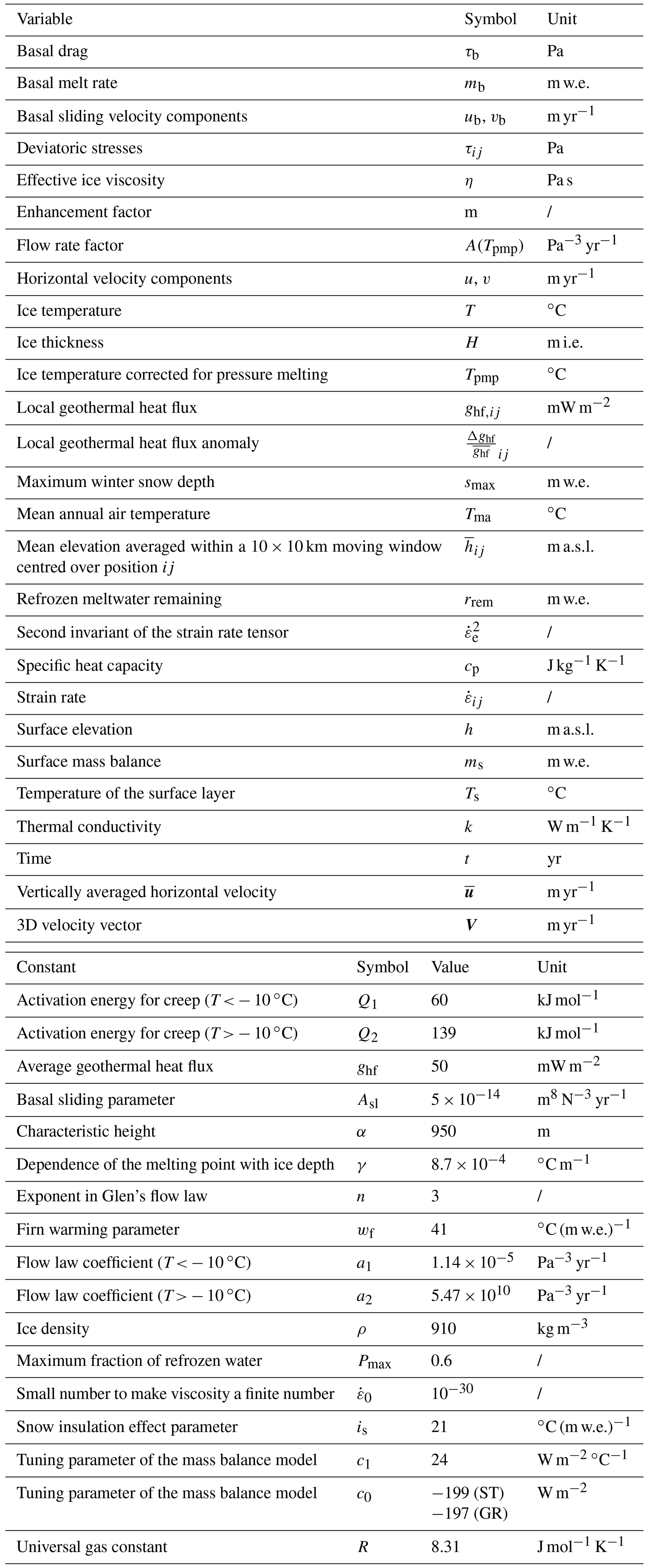
Table 1 Variables and constants and their symbols, values, and units. ST refers to the Sary-Tor glacier, while GR stands for the Grigoriev ice cap.

3.3 Boundary conditions

The calculation of the ice temperature distribution requires the specification of two boundary conditions: the ice temperature of the surface layer and the temperature gradient at the bottom of the ice masses.

3.3.1 Basal boundary conditions

At the bottom, heat is produced by geothermal heating (energy received by the ice at its base) and friction induced by basal sliding and ice deformation. Heat flow studies at regional scales in the Kyrgyz Tien Shan indicate the presence of a “cold Cenozoic orogeny” with no additional heating associated with tectonic deformation and basin development. The area is characterised by an average geothermal heat flux ($\stackrel{\mathrm{‾}}{g_{\mathrm{hf}}}$) of approximately 50 mW m⁻² (Duchkov et al., 2001; Vermeesch et al., 2004; Bagdassarov et al., 2011; Delvaux et al., 2013). This is on the same order as the value used for the modelling of glacier no. 8 in the Hei valley in China (Wu et al., 2019) and for Abramov glacier (Barandun et al., 2015). This corresponds to a basal temperature gradient of 0.024 ^∘C m⁻¹ for a typical thermal conductivity of 2.1 W m^−1 ∘C⁻¹. To account for the influence of topography on the geothermal heat flux, we apply the empirically determined topographic correction procedure described in Colgan et al. (2021). This concerns a high-pass filter with a dimensionless correction factor applied to the average geothermal heat flux, which makes the geothermal heat flux spatially variable depending on the local elevation (h_ij). Using the correction factor, the geothermal heat flux is magnified in incised valleys such as for the Sary-Tor glacier and attenuated on ridges such as for the Grigoriev ice cap. More specifically, in the correction procedure, the average geothermal heat flux is perturbed by an anomaly (${\frac{\mathrm{\Delta }{g}_{\mathrm{hf}}}{\stackrel{\mathrm{‾}}{g_{\mathrm{hf}}}}}_{ij}$) to obtain the local geothermal heat flux (g_hf,ij).

$$\begin{array}{}\text{(14)}& g_{\mathrm{hf},ij}=\stackrel{\mathrm{‾}}{g_{\mathrm{hf}}}\left(\mathrm{1}+{{\displaystyle \frac{\mathrm{\Delta }{g}_{\mathrm{hf}}}{\stackrel{\mathrm{‾}}{g_{\mathrm{hf}}}}}}_{ij}\right)\end{array}$$

The anomaly is estimated as a function of local relief using

$$\begin{array}{}\text{(15)}& {{\displaystyle \frac{\mathrm{\Delta }{g}_{\mathrm{hf}}}{\stackrel{\mathrm{‾}}{g_{\mathrm{hf}}}}}}_{ij}={\displaystyle \frac{\mathrm{1}}{\mathit{\alpha }}}({\stackrel{\mathrm{‾}}{h}}_{ij}-h_{ij}),\end{array}$$

with α an empirically determined characteristic height (950 m) and ${\stackrel{\mathrm{‾}}{h}}_{ij}$ the mean elevation averaged within a moving window of 10 × 10 km centred over location ij. Then, as a boundary condition at the bed, the temperature gradient is defined as the sum of the local geothermal heat flux and the heat due to basal sliding (Huybrechts and Oerlemans, 1988):

$$\begin{array}{}\text{(16)}& {\displaystyle \frac{\partial T}{\partial z}}=-{\displaystyle \frac{g_{\mathrm{hf},ij}+{\mathit{\tau }}_{\mathrm{b},\mathrm{u}}{u}_{\mathrm{b}}+{\mathit{\tau }}_{\mathrm{b},\mathrm{v}}{v}_{\mathrm{b}}}{k}}.\end{array}$$

τ_b is the basal shear stress, u_b and v_b are the basal velocity components, and k is the thermal conductivity.

3.3.2 Surface boundary conditions

As an upper boundary condition, the ice temperature of the surface layer is usually set equal to the mean annual air temperature (T_ma) (Loewe, 1970; Hooke et al., 1983; Zekollari et al., 2017). This is a good approximation for the cold and dry accumulation area (the part of the accumulation area without substantial melt). However, the T_ma has been proven to be a major underestimate for the infiltration congelation/recrystallisation zone, which is the part of the accumulation area where snowmelt occurs and where the meltwater refreezes again (Shumskiy, 1955; Hooke, 1976; Maohuan et al., 1982; Maohuan, 1990; Arkhipov et al., 2004; van Pelt et al., 2016; Zekollari et al., 2017; Kronenberg et al., 2021). Latent heat released through water percolation and refreezing in firn induces warming (Shumskiy, 1955; Maohuan, 1990; Huybrechts et al., 1991; van Pelt et al., 2016; Zekollari et al., 2017). Heat conduction and advection expands this warm signal, which is often called cryo-hydrological warming (Lüthi et al., 2015). It is important to take this effect into account, which raises the temperatures, relaxing associated viscosity and hence increasing local flow velocities (Colgan et al., 2015). To consider the effect of meltwater refreezing and its warming effect on the surface layer, a parameterisation is applied that warms the surface layer for the locations where meltwater refreezes and remains at the end of a mass balance year (Reeh, 1991; Huybrechts et al., 1991; Zekollari et al., 2017). Below the equilibrium line, this latent heat is lost together with meltwater runoff over the impermeable ice surface.

However, besides a warming effect due to refreezing meltwater, other processes play a role in determining the ice temperature of the surface layer. The presence or absence of snow has been proven to be crucial for the surface layer temperature (Hooke et al., 1983; Zhang, 2005; Meierbachtol et al., 2015). The most pronounced effect of snow on the surface layer temperature of ice masses occurs in the winter. During the winter months, because of the lower thermal conductivity of snow compared to ice, a significant snow cover insulates the ice below as a blanket from the strongest winter cold penetrating the ice (Hooke et al., 1983; Zhang, 2005; Kronenberg et al., 2021). This ensures that average temperatures below the snow cover are usually much higher compared to the average air temperatures above the snow (Hooke et al., 1983).

In addition to the effect of the insulating snow layer, in the ablation area, the vertical velocity is positive (upward), implying that ice from deeper layers is advected upwards. Further, the upper ice layers are removed due to melting. Both these processes ensure that the ice temperature of the surface layer in the ablation area is strongly influenced by the ice temperature of the deeper layers (upward vertical advection). For this reason, Wohlleben et al. (2009) and Blatter (1987) proposed using the ice temperature gradient to prescribe the ice temperature of the surface layer as a boundary condition. However, this still requires a prescription of the air temperature that influences the ice surface temperature from above.

A last effect that can influence the surface layer temperature is the percolation of water through crevasses and moulins. This water can provide heat of friction or it can refreeze, contributing to ice temperature warming (Phillips et al., 2010; Gilbert et al., 2020). These processes are not considered in this study because significantly large areas with crevasses or moulins were detected for neither the Grigoriev nor for the Sary-Tor glacier. Observations show that meltwater on both ice masses is mainly discharged supraglacially.

Different methods have been used to determine the surface boundary condition, accounting for snow cover and mean July temperatures for the ablation area and the percolation zone (Hooke et al., 1983) or by solely using a firn warming effect in the accumulation area (Zekollari et al., 2017). Here, we apply a combination of both, resulting in a simple parameterisation with two tuning parameters implicitly accounting for the effects of refreezing meltwater and snow insulation, which are described above:

$$\begin{array}{}\text{(17)}& T_{\mathrm{s}}=\begin{array}{l}min(\mathrm{0}{}^{\circ }\mathrm{C},T_{\mathrm{ma}}+w_{\mathrm{f}}{r}_{\mathrm{rem}}+i_{\mathrm{s}}{s}_{\max })\\ h>\mathrm{ELA}\\ min(\mathrm{0}{}^{\circ }\mathrm{C},T_{\mathrm{ma}}+i_{\mathrm{s}}{s}_{\max }+m_{\mathrm{s}}(\text{in}\mathrm{m}\mathrm{i}.\mathrm{e}.\left)\frac{T_{\mathrm{20}\mathrm{m}}-T_{\mathrm{10}\mathrm{m}}}{\mathrm{10}\left(\mathrm{m}\mathrm{i}.\mathrm{e}.\right)}\right)\\ h<\mathrm{ELA}.\end{array}\end{array}$$

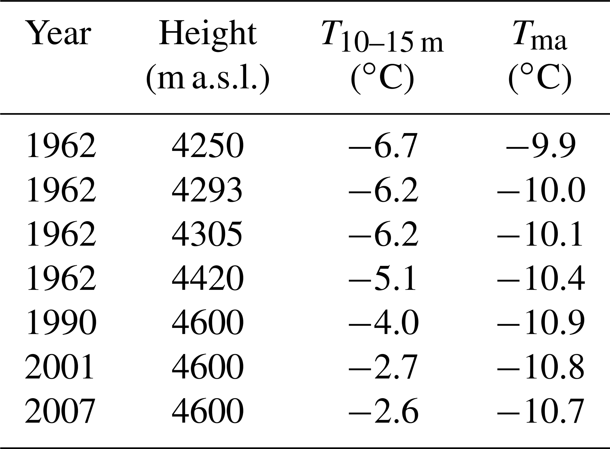
T_s is the ice temperature of the surface layer, which is assumed not to be influenced by the seasonal cycle. Hence, it corresponds typically to the ice temperature at 10–15 m depth. T_s is used as the upper boundary condition in the model. T_ma is the mean annual air temperature, which is calculated by taking the average values of all hours in 1 year. For the lapse rate, a sinusoidal function is used with a limit of −0.0065 in June and −0.0023 ^∘C m⁻¹ in January, based on data from Aizen et al. (1995), to ensure a smooth transition of the lapse rates during the year. For the calculation of T_ma, as for the mass balance model (see Sect. 3.4), temperature data from the Kumtor–Tien Shan meteorological station (Fig. 1) are used (see Van Tricht et al., 2021b, for more information about this meteorological station); w_f corresponds to the firn warming parameter (^∘C (m w.e.)⁻¹), which determines the warming for every metre of refrozen meltwater remaining (r_rem) at the end of each mass balance year. The i_s parameter (^∘C (m w.e.)⁻¹) corresponds to the snow insulation effect based on the maximum snow depth at the end of spring (s_max), when snow thickness on the ice masses is typically at a maximum. When the ice temperature of the surface layer reaches the melting temperature, the ice temperature is kept constant at 0 ^∘C. The temperature gradient between 10–20 m ice depth ($(T_{\mathrm{20}\mathrm{m}}-T_{\mathrm{10}\mathrm{m}})/\mathrm{10}$) and the surface mass balance (m_s) are used to correct for the effect of surface layer removal in the ablation area. Both the w_f and i_s parameters are calibrated based on historical and spatially distributed ice temperature measurement at 10–15 m depth (assumed to reflect the average annual temperature) on the Grigoriev ice cap (Dikikh et al., 1965; Thompson et al., 1993; Arkhipov et al., 2004; Takeuchi et al., 2014) (Table 2 and Sect. 2.2). The calibrated mass balance model (see Sect. 3.4) is used to estimate the average amount of r_rem at the end of the year and s_max. The 15 years prior to each of the individual measurements in Table 2 are used for the average values of T_ma, r_rem, and s_max. This period is chosen because it is large enough to filter out interannual variability and at the same time considers sufficient fluctuations in the conditions at the surface. An overview of the temperature measurements used for calibration in this study (see Sect. 3.3) is given in Table 2. As can be seen in Table 2, the ice temperatures at 10–15 m depth increase with altitude, while the mean annual air temperatures decrease with altitude. This difference can be explained by the effect of an increasing warming of the surface layer due to refreezing meltwater and maximum snow thickness for insulation.

Table 2 Measured ice temperatures of the Grigoriev ice cap at 10–15 m depth from 1962 (Dikikh et al., 1965), 1990 (Thompson et al., 1993), 2001 (Arkhipov et al., 2004), and 2007 (Takeuchi et al., 2014). T_ma represents the mean annual air temperature at the considered surface elevation of the 15 years prior to each individual measurement.

3.4 Mass balance model

To obtain m_s, s_max, and r_rem, we apply the surface energy mass balance model that has been optimised, calibrated, and used in Van Tricht et al. (2021b). This simplified model is based on incoming solar radiation, temperature, and precipitation and contains two additional tuning parameters (c₀ and c₁), representing the sum of the net longwave radiation balance and the turbulent sensible heat exchange. The temporal resolution of the mass balance model is 1 h, while the coupling with the ice flow model occurs yearly. The input data of the mass balance model are limited to a digital elevation model (DEM), air temperatures, and solid precipitation at hourly intervals. For meteorological data, the reconstructed data series of the Kumtor–Tien Shan meteorological station is used (Van Tricht et al., 2021b). The DEM is used to calculate the hourly (solar) insolation with respect to the slope and aspect of every grid point and the effect of shadow, needed for the energy balance, and to estimate the temperature and precipitation based on the absolute elevation of the grid point. For the Sary-Tor glacier, we directly use the calibrated parameters (c₀ and c₁) from Van Tricht et al. (2021b). However, incorporating the mass balance measurements from 2020/21 in the calibration procedure reveals an optimal c₀ value of −199, which is slightly lower than the obtained value of −193 based on calibration data from 2014–2020. Concerning the Grigoriev ice cap, initially, the same parameters are used as for the Sary-Tor glacier. The c₁ parameter is fixed at 24 as this was found to be optimal for the other glaciers in the area (Van Tricht et al., 2021b). However, the c₀ parameter and the precipitation gradient are then tuned by minimising the root mean square error (RMSE) between modelled and measured mass balances from Dyurgerov (2002), Arkhipov et al. (2004), and Fujita et al. (2011) (Table 3). For instance, Arkhipov et al. (2004) determined the average accumulation at the summit of the Grigoriev ice cap based on the detection of annual layers to be 0.26 m w.e. yr⁻¹ between 1990 and 2000, which appeared to be slightly less than the 0.32 m w.e. yr⁻¹ between 1963 and 1989.

Table 3 Data used for the calibration of the mass balance model for the Grigoriev ice cap; m_s represents the surface mass balance.

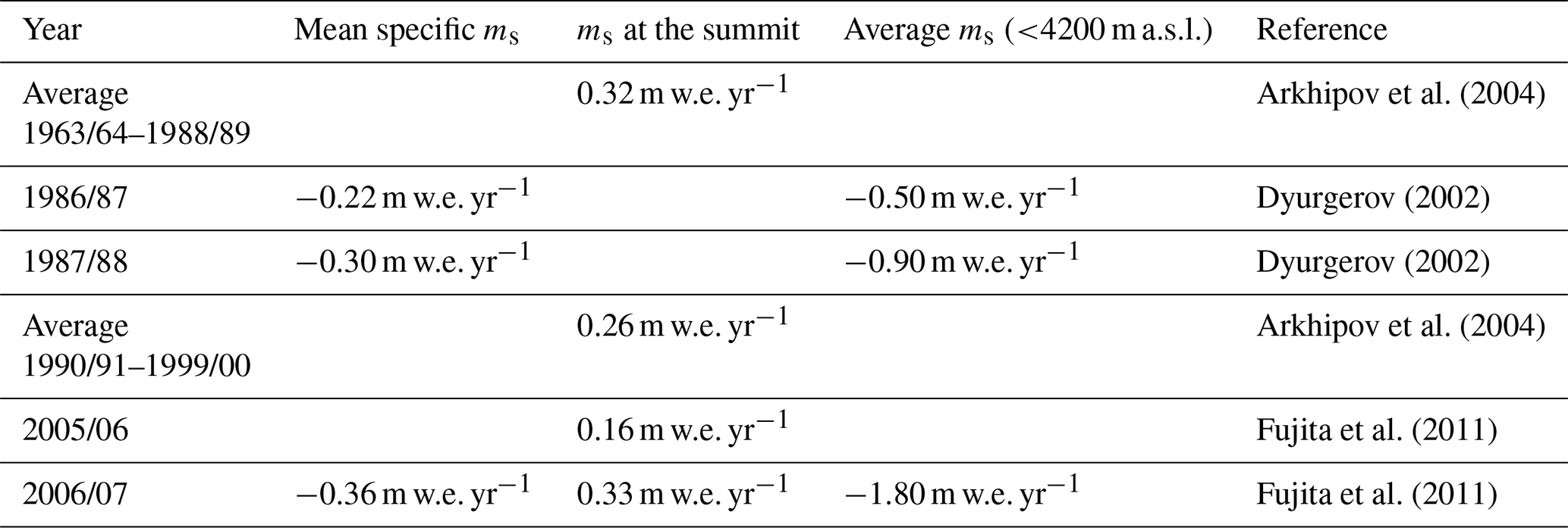
The calibration of the mass balance model for the Grigoriev ice cap reveals optimal values for a precipitation gradient of +150 mm km⁻¹ yr⁻¹ and a c₀ value of −197 W m⁻². This rather low value for the precipitation gradient (compared to the Sary-Tor glacier) appears to be necessary to limit the accumulation on the summit of the ice cap, as was measured and reconstructed by Arkhipov et al. (2004) and Fujita et al. (2011). Such a low gradient can be explained by the location of the Grigoriev ice cap on the top of an isolated mountain, lower than the surrounding mountains, reducing the effect of orographic precipitation enhancement and making it more exposed to wind erosion. On the other hand, the Sary-Tor glacier is located at the north-western side of the Ak-Shyirak massive, which could be more exposed to precipitation. The calibrated c₀ value is of equal magnitude compared to the values found for the Bordu and Sary-Tor glaciers located nearby (Van Tricht et al., 2021b).

A crucial output of the mass balance model for the determination of the thermal regime is the amount of meltwater that refreezes in the snowpack (see Sect. 3.3). Following Van Tricht et al. (2021b), we assume all snowmelt to percolate into the snow cover and to be retained and to refreeze until a maximum amount of P_max (taken as 60 % of the snow depth) is reached (Reeh, 1991; Huybrechts et al., 1991). At every time step, the snow depth and the amount of refrozen water are updated. Finally, at the end of the mass balance year, it is assumed that the remaining refrozen meltwater forms r_rem. Refreezing of meltwater below the last summer horizon can occur if not all pore spaces of the existing snow cover are occupied (<60 %), as was shown to be an important process for glaciers and ice caps in the area (Dyurgerov and Mikhalenko, 1995; Takeuchi et al., 2014; Kronenberg et al., 2016). The maximum snow depth s_max is determined by considering the maximum snow depth before the end of May when average snow depths are typically maximal on glaciers in the area (Van Tricht et al., 2021c). During the summer months, regular snow events can still occur during convective showers, but melt then compensates for the accumulation so that the snow thicknesses on the ice masses usually no longer increase, and snow insulation is focused on winter and spring.

3.5 Geometric data

Several geometric datasets are needed to apply the ice dynamic model and the surface mass balance model. The experiments in this study are performed under average 1960–1990 climatic conditions. Therefore, the geometry of the Grigoriev ice cap and the Sary-Tor glacier is reconstructed for 1990 as a starting point for all simulations.

3.5.1 Outlines

The outlines of both ice masses are initially taken from the Randolph Glacier Inventory v6 (RGI, 2017). Subsequently, optical satellite images from Landsat 5, valid for August 1990, are used to update the outline using manual delineation based on visual inspection of the ice–bedrock boundary. Furthermore, a LIA ice mask is created from visual detection of unique LIA moraines, clearly present in satellite images (Landsat and Sentinel-2) for both the Grigoriev ice cap and the Sary-Tor glacier. This ice mask serves as the maximum area of both ice masses which is allowed to be occupied by ice. If the ice were to expand beyond the mask, the ice would be removed. However, this never applies to the geometry for average 1960–1990 climatic conditions as this remains entirely within the LIA mask. Concerning the northern boundary of the Grigoriev ice cap, when ice flows beyond the predefined calving front, it is automatically removed.

3.5.2 Bedrock DEM

Concerning the Sary-Tor glacier, the ice thickness measurements were performed with a VIRL-6 GPR radar at 20 MHz central frequency (Petrakov et al., 2014). A maximum part of the accessible area of the glacier was covered with a grid of longitudinal and transverse profiles. Then, an ice thickness field was reconstructed using interpolation with an estimated accuracy of 15–20 m, and a volume of 0.126 ± 0.001 km³ was obtained (Petrakov et al., 2014). A bedrock DEM is obtained by subtracting the ice thickness of Sary-Tor glacier in 2013 from the surface elevation in 2013 (obtained from the TanDEM-X DEM). Corrected for ice melt between 2013 and 2021, a maximum ice thickness of 157 ± 15 m and a total ice volume of 0.118 ± 0.001 km³ in 2021 are obtained. Concerning the ice thickness of the Grigoriev ice cap, we performed ∼ 500 GPR measurements over the entire ice cap in the summer of 2021 using a Narod radio echo sounding system with a lower frequency of 5 MHz, reducing the necessity for interpolation over larger distances between the measurement transects (Fig. 2). A maximum ice thickness of 114 ± 10 m was measured. Subsequently, following Van Tricht et al. (2021a), a glacier-wide ice thickness field was reconstructed using a constant yield stress model for the unmeasured areas, resulting in a total ice volume of 0.391 ± 0.07 km³. During the field campaign, unpiloted aerial vehicle (UAV) images were collected using a DJI Phantom 4 RTK from about 200 m above the ice cap. These images were subsequently used in Pix4D to infer an accurate and centimetre-resolution digital surface model (DSM), as in Van Tricht et al. (2021c). A bedrock DEM is determined by subtracting the reconstructed ice thickness distribution from the DSM.

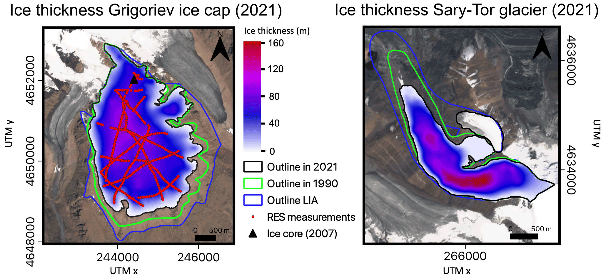
Figure 2 Ice thickness distribution of the Grigoriev ice cap and the Sary-Tor glacier in 2021. The locations of the ice thickness measurements of 2021 on the Grigoriev ice cap are added in red. The background is a Sentinel-2 image from 26 July 2021. The location of the ice core made in 2007 (Takeuchi et al., 2014) is added with a black triangle.

3.5.3 DEM of 1990

For consistency with the 1960–1990 climatic conditions, a DEM is created for 1990 as an initial state to be used in the glacier model. Using the calibrated mass balance model (see Sect. 3.4), the cumulative mass balance is calculated between 1990 and the year in which the ice thickness was measured (2021 for the Grigoriev ice cap and 2013 for the Sary-Tor glacier). Under the assumption that ΔSMB =ΔH (hence neglecting the role of ice dynamics for these periods), the surface elevation of 1990 is then inferred by adding ΔSMB to the DEM of 2021 and 2013 for the glacial area (Fig. 3). Outside the glacial area of 2013 and 2021, the surface elevation is reconstructed by setting the elevation equal to the bedrock elevation at the 1990 front, attaching to the DEM of 2013/2021 at the observed glacier front and interpolating in between (Fig. 3).

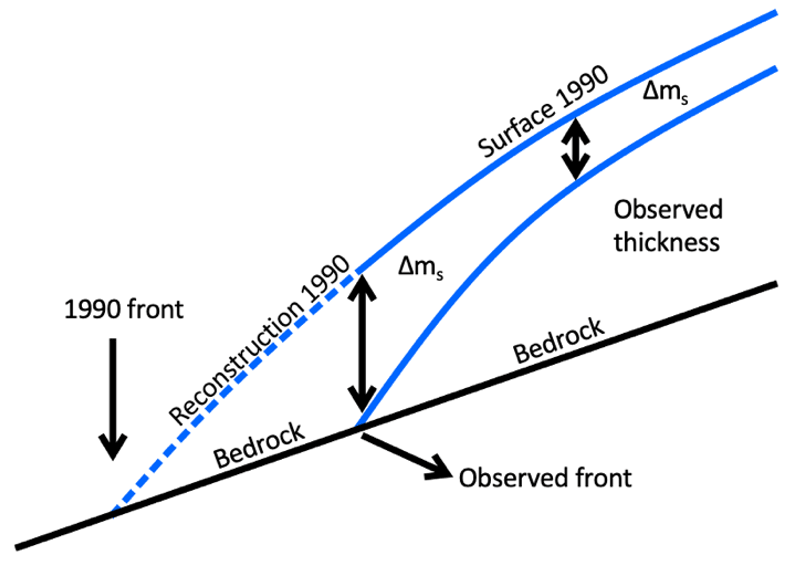
Figure 3 Reconstruction of the 1990 geometry from a combination of modelling the cumulative surface mass balance (Δm_s) and interpolation.

Reconstructed for the 1990 geometry, we obtain an area of the Grigoriev ice cap of 8.746 ± 0.42 km² (∼ 15 % larger than the present-day area), with a maximum ice thickness of 115 ± 10 m and a total ice volume of 0.513 ± 0.11 km³ (∼ 30 % more than the present-day volume). The corresponding values for the Sary-Tor glacier are an area of 2.789 ± 0.22 km² (∼ 21 % larger than the present-day area), a maximum ice thickness of 158 ± 15 m, and a total volume of 0.158 ± 0.002 km³ (∼ 34 % more than the present-day volume). Hence, both ice bodies lost a substantial fraction of their area and volume over the last 31 years, similar to observations in other studies (Aizen et al., 2006; Kutuzov and Shahgedanova, 2009; Sorg et al., 2012). Created for 1990, the geometry of both ice masses is used to initiate the experiments below. The eastern tributary of the Sary-Tor glacier (visible in the right panel of Fig. 2) is not included for the 1960–1990 runs, as it was already disconnected from the Sary-Tor main glacier at the end of this time frame.

3.6 Experiments and sensitivity analysis

First, multiple experiments are performed using the coupled surface mass balance and the ice flow models with standard settings for the basal sliding parameter A_sl (5.10⁻¹⁴ m⁸ N⁻³ yr⁻¹; see Table 1). The velocity and temperature fields are run under constant 1960–1990 climatic conditions. During the runs, the geometry is freely evolving with a maximum limit of the LIA extent, until a steady state is reached. When a steady state is reached, modelled ice thickness is compared with the 1990 reconstructed thickness, and temperature fields are compared with measured temperatures as well as with detected boundaries between cold and temperate ice (Petrakov et al., 2014). A constant mass balance correction over the entire ice mass is implemented to reach the extent of the 1990 geometry.

Then, a sensitivity analysis is performed with regards to the different parameters affecting the temperature distribution in the ice masses. This specifically concerns the i_s and w_f parameters, which are altered within ±10 %. In each run, one parameter is changed, while the other remains fixed at its optimal value. The sensitivity with regard to the geothermal heat flux is also assessed by using 50 % and 200 % of the average geothermal heat flux. In every experiment, the geometry is first freely evolving until a steady state is reached using the optimal parameter values. Then, the parameter under consideration is altered, and the geometry is kept fixed to avoid an effect of a thinner or thicker ice mass caused by a change in the ice viscosity and to simplify the interpretation of the results.

Finally, a sensitivity to changes in boundary conditions is investigated by altering the precipitation −40 % to 40 % and the surface temperatures −2 to +3 ^∘C. These ranges were selected based on observed (Van Tricht et al., 2021b) and projected changes for the area. For this analysis, the geometry can evolve freely until a new steady state is reached in equilibrium with the altered surface boundary conditions. This analysis can give an indication about the evolution of the thermal regime in the past and into the future, which is part of the “Results and discussion” section.

4 Results and discussion

4.1 Surface mass balance

Based on the calibrated surface mass balance model and the average climatic conditions of 1960–1990, at similar elevation, the ablation is about 1 m w.e. yr⁻¹ more negative for the Grigoriev ice cap compared to the Sary-Tor glacier, which is due to the orientation (mostly south vs. north-west) and the lower amount of precipitation. The estimated equilibrium line altitude (ELA) for the 1960–1990 period is around 4300 m a.s.l. for the Grigoriev ice cap, which is close to the average ELA found in Arkhipov et al. (2004), and is about 4200 m a.s.l. for the Sary-Tor glacier. For average 1960–1990 climatic conditions, the mean specific mass balance is +0.15 m w.e. yr⁻¹ for the Grigoriev ice cap and −0.06 m w.e. yr⁻¹ for the Sary-Tor glacier (Fig. 4). For the experiments with the ice flow model, the surface mass balance of the Sary-Tor glacier is adjusted by adding +0.08 m w.e. yr⁻¹, and the surface mass balance of the Grigoriev is adjusted by −0.05 m w.e. yr⁻¹ to obtain a steady state with an extent as close as possible to the extent of the reconstructed 1990 geometry (see Sect. 4.3). This mass balance correction implies that the reconstructed ice masses for 1990 are not totally in equilibrium with the 1960–1990 climatic conditions.

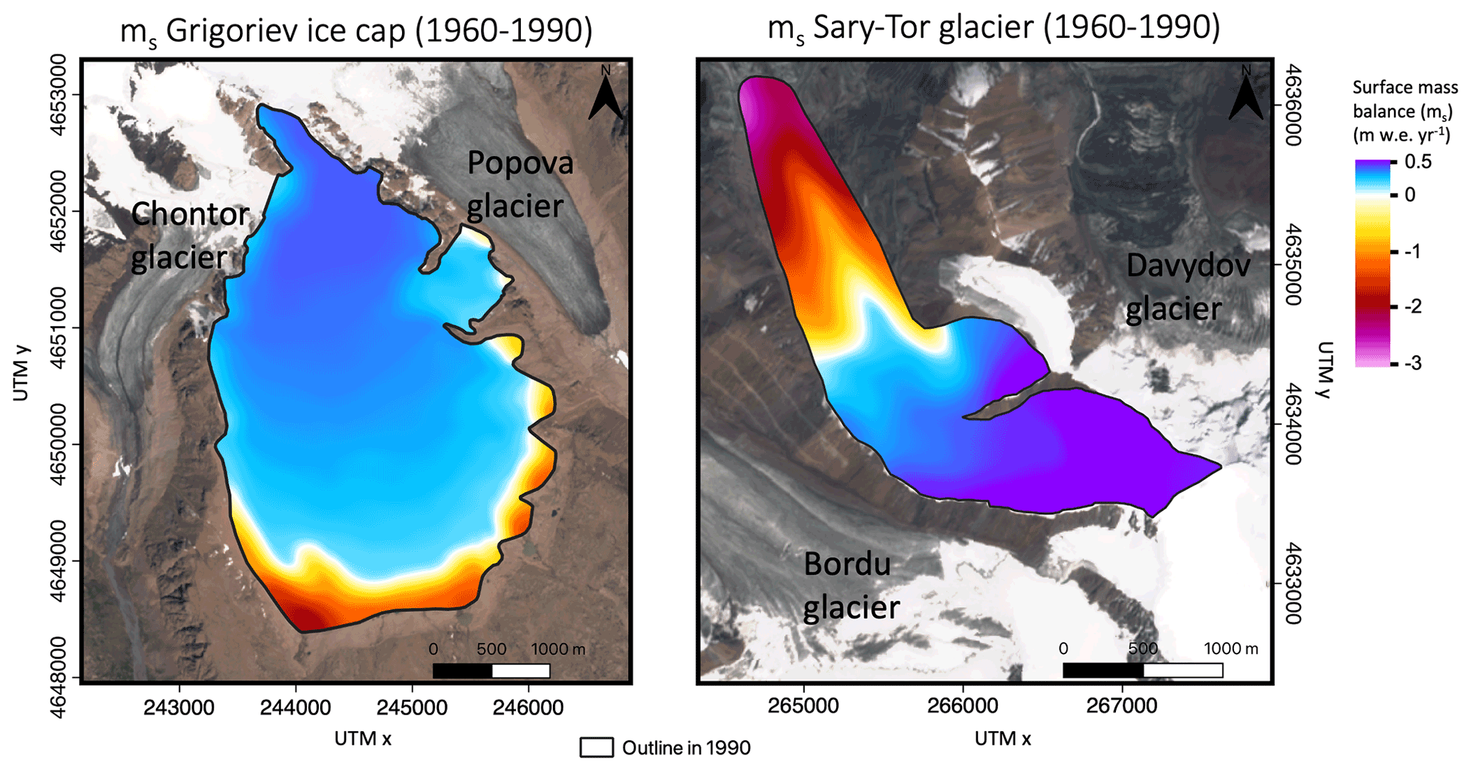
Figure 4 Average surface mass balance (m_s; m w.e. yr¹) of the Grigoriev ice cap and the Sary-Tor glacier for the mean 1960–1990 climatic conditions. The background is a Sentinel-2 image from 26 July 2021.

4.2 Boundary conditions

4.2.1 Firn warming and snow insulation

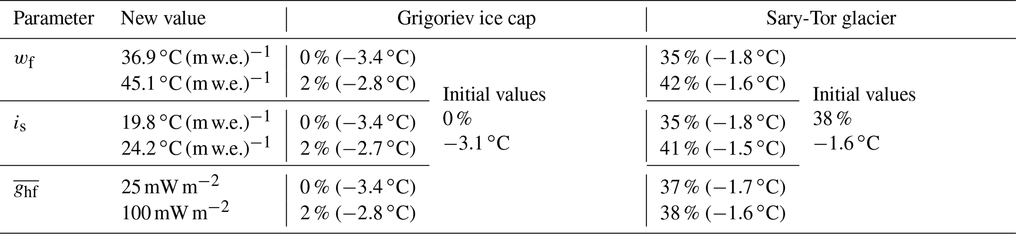
Using the output from the surface mass balance model, r_rem and s_max, and the temperature data, the optimal combination of the w_f and the i_s parameters is 41 and 22 (^∘C (m w.e.)⁻¹) (Fig. 5a). The corresponding RMSE between the measured (see Table 2) and modelled temperatures at 10–15 m depth is equal to 0.28 ^∘C (Fig. 5a, b), which is a close correspondence.

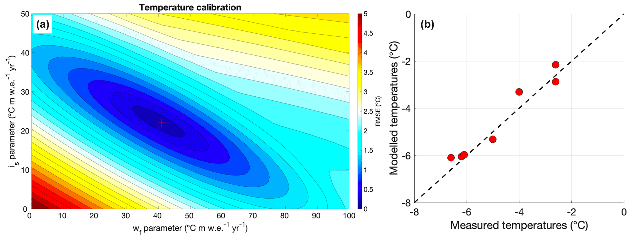
Figure 5 (a) Calibration of the w_f and the i_s parameters based on ice temperature measurements of the Grigoriev ice cap. (b) Modelled and measured temperatures for different elevations and times of the Grigoriev ice cap.

The obtained firn warming parameter (w_f) value (41 ^∘C (m w.e.)⁻¹) is larger than values found in previous studies, for example, for the Greenland ice sheet (26.6 ^∘C (m w.e.)⁻¹; Reeh, 1991; Huybrechts et al., 1991) and Hans Tausen ice cap (22 ^∘C (m w.e.)⁻¹; Zekollari et al., 2017). The parameter to consider for the insulation of snow (optimal i_s=22 ^∘C (m w.e.)⁻¹) is slightly larger than the values found in Hooke et al. (1983) (about 4 ^∘C for 1 m of snow (∼ 12–20 ^∘C (m w.e.)⁻¹ yr⁻¹) on the Storglaciären glacier, or about 2.5 ^∘C warming for 0.6 m of snow (∼ 13–21 ^∘C (m w.e.)⁻¹ yr⁻¹) for the Barnes ice cap). However, Zhang (2005) and Yershov (1998) reported a mean annual temperature increase of about 0.1 ^∘C cm⁻¹ of snow, which is equivalent to 10 ^∘C m⁻¹ yr⁻¹ of snow (∼ 30–50 ^∘C (m w.e.)⁻¹ yr⁻¹). In the applied model, the calibrated values of w_f and i_s are kept constant in space and time.

4.2.2 Surface warming and temperatures

The input of latent heat from percolating and refreezing meltwater is the strongest in the middle part of the accumulation zones (Fig. 6) (infiltration congelation/recrystallisation zone). At the highest elevations, the amount of refrozen water is low, caused by the absence of substantial melt (too low temperatures). This area corresponds to the dry snow zone or recrystallisation zone (Shumskiy, 1955). The effect related to snow insulation is more homogeneously distributed over the ice bodies (Fig. 6) because almost all precipitation in winter and spring is snow, independent of the elevation on the glacier, which ensures that differences in maximum snow depth at the end of spring are only related to precipitation enhancement with elevation. Combining the effect of firn warming and snow insulation, an entirely cold surface condition is obtained for the Grigoriev ice cap, while a polythermal surface condition is obtained for the Sary-Tor glacier (Fig. 6).

For both ice masses, the coldest ice temperatures at the surface can be found in the ablation areas, where the formation of superimposed ice at the end of summer is absent because the meltwater is evacuated and where a thinner snow cover in winter allows for a larger surface cooling (Fig. 6). The temperatures are the highest in the accumulation areas. Concerning the Sary-Tor glacier, there is a temperate band between ∼ 4200–4500 m with temperatures equal to 0 ^∘C. The hypothesis is that these higher ice temperatures are dissipated downwards through conduction and vertical movement towards lower elevations, causing the expected polythermal regime of the valley glaciers (Petrakov et al., 2014), as also observed on the Tuyuksu glacier in the northern Tien Shan (Nosenko et al., 2016). At the highest elevations of the Sary-Tor glacier, the ice temperature at the surface are again lower because of the absence of meltwater available for refreezing.

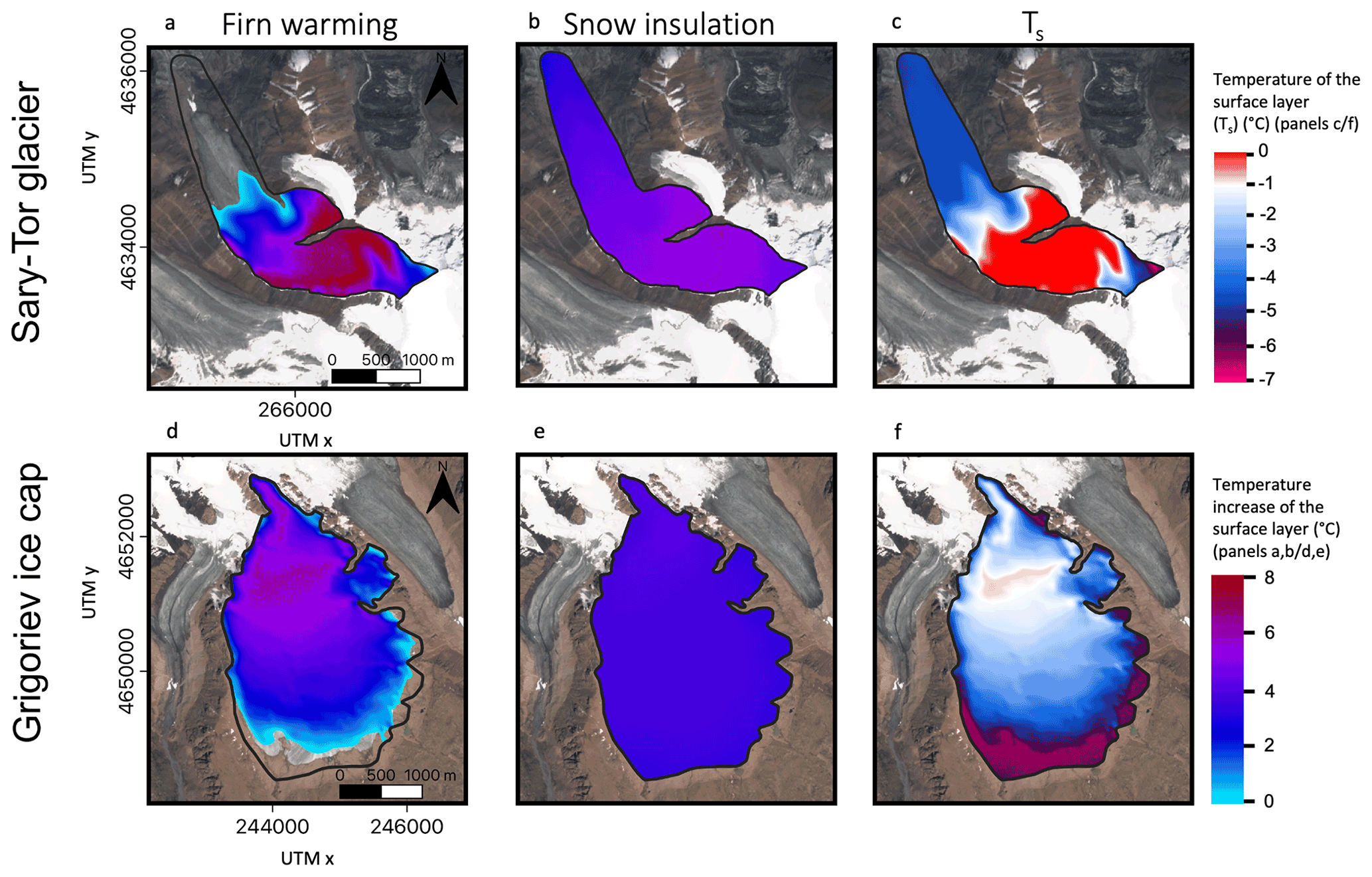
Figure 6 Warming due to refreezing of meltwater (firn warming) (panels a and d), due to snow insulation (panels b and e) and resulting mean annual surface layer temperature (T_s) (panels c and f) for both ice masses according to constant 1960–1990 average climatic conditions and masked for the 1990 outline (black lines). The background is a Sentinel-2 image from 26 July 2021. The x and y axes in (a) and (d) apply to the other panels as well.

4.3 Modelled steady-state velocities and thickness

Under constant 1960–1990 climatic conditions and with the applied surface mass balance adjustments, the obtained steady states match the reconstructed 1990 geometry (extent and ice thickness) relatively well (Fig. 7). The RMSE between the reconstructed and modelled ice thickness is about 22.01 m for the Sary-Tor glacier and 15.20 m for the Grigoriev ice cap. The enhancement factor is set at 3 for the Grigoriev ice cap and at 4 for the Sary-Tor glacier, which appears to be the optimal value to match with the reconstructed ice thickness of 1990. For the Sary-Tor glacier, in general, modelled and reconstructed ice thickness match well (Fig. 7), and discrepancies mainly occur in areas where no GPR measurements were performed (Petrakov et al., 2014). Regarding the Grigoriev ice cap, the modelled ice thickness is slightly thicker and generally extends farther at the edges of the ice cap compared to the 1990 reconstruction. At the top, on the other hand, the modelled ice thickness is thinner (15–25 m). The latter might be associated with the complexity of modelling ice thickness in the vicinity of ice divides (Pattyn, 2003) or with the measurements of the ice thickness itself. It is unlikely that the underestimated modelled ice thickness at the top of the Grigoriev ice cap is related to an excessively high ice temperature, as correctly modelling the ice thickness here would require an enhancement factor of 1, which corresponds to a lower temperature of −5 ^∘C (Huybrechts and Oerlemans, 1988). This is far outside the limit of the values of the observed ice temperatures (Thompson et al., 1993; Arkhipov et al., 2004; Takeuchi et al., 2014).

Figure 7 (a, c) Ice thickness difference between the modelled steady state (∼ 1960–1990 average climatic conditions) and the reconstructed geometry of 1990. The used flowline is added on the map with a black line. (b, d) Reconstructed (initial glacier surface) and modelled (glacier surface) ice thickness along the central flowlines. Panels (a) and (b) are for the Sary-Tor glacier, and panels (c) and (d) are for the Grigoriev ice cap. The background of the left maps is a Sentinel-2 image from 26 July 2021. The outlines are from 1990.

Regarding the horizontal (surface) ice velocities, the Grigoriev ice cap is generally characterised by a very low velocity between 0 and 5 m yr⁻¹ (Fig. 8c). Such low values were also observed by Fujita et al. (2011) and modelled by Nagornov et al. (2006). The very low ice velocities imply that the ice is only advected very slowly downstream, keeping ice fluxes low. Only for the outlet glacier in the eastern part, which flows towards the Popova glacier, do velocities increase to >20 m yr⁻¹ due to the steeper slope in this area. The ice velocities are mostly significantly higher for the Sary-Tor glacier with a maximum slightly above 30 m yr⁻¹ (Fig. 8). This implies that the horizontal advection of ice for Sary-Tor glacier is much more pronounced. Comparison between modelled velocities and velocities derived from mass balance stake displacements at the Sary-Tor glacier shows a close correspondence (RMSE = 1.5 m yr⁻¹).

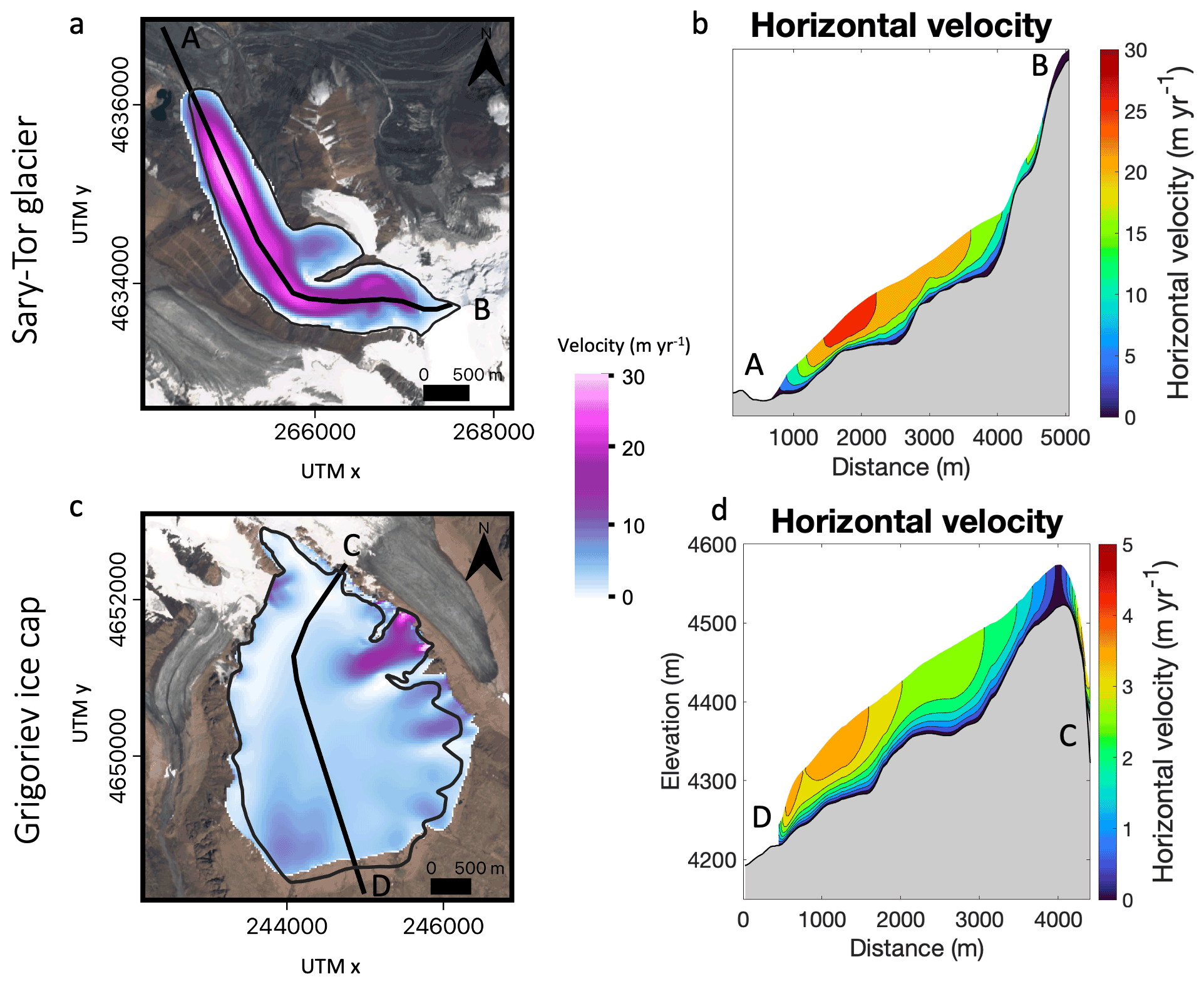
Figure 8 (a, c) Horizontal surface ice velocities of the Grigoriev ice cap and the Sary-Tor glacier. The flowline is added on the map with a black line. (b, d) Horizontal ice velocities along the flowlines of both ice masses. Panels (a) and (b) are for the Sary-Tor glacier, and panels (c) and (d) are for the Grigoriev ice cap. The background of the left maps is a Sentinel-2 image from 26 July 2021. The outlines are from 1990.

4.4 Thermal regime under the 1960–1990 climatic conditions

With the imposed boundary conditions and the modelled thickness and velocity structure, the steady-state englacial ice temperatures are determined. They range between −7.70 and 0 ^∘C for the Sary-Tor glacier and between −6.61 and −0.03 ^∘C for the Grigoriev ice cap. A polythermal regime is obtained for the Sary-Tor glacier (Fig. 9). Temperate ice is present over a large part of the glacier base, originating in the accumulation area, which is subsequently advected downstream with the ice flow. At the snout of the Sary-Tor glacier and in the largest part of the ablation area, the ice is cold. Over the entire glacier volume, about 38 % of the ice of the Sary-Tor glacier is temperate, classifying this glacier reliably as a polythermal glacier. Concerning the Grigoriev ice cap, the model results show cold ice except for a very thin layer at the bed in the central part, which is characterised by temperate ice. This concerns less than 1 % of the total volume. Hence, the Grigoriev ice cap can be classified as a cold ice cap. The thin layer of temperate ice in the central area at the bed was also observed on GPR profiles measured by Ivan Lavrentiev in 2018 (personal communication in 2022), increasing the confidence in the obtained results.

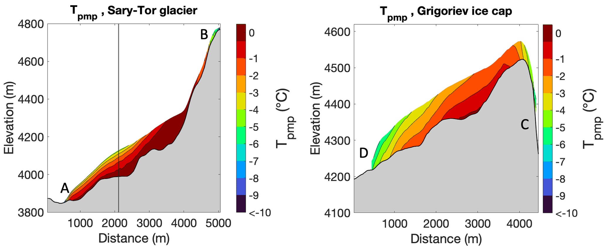
Figure 9 Modelled ice temperatures of the Sary-Tor glacier and the Grigoriev ice cap along the central flowline using a freely evolving geometry and corrected for the pressure melting point. The vertical line in the plot of the Sary-Tor glacier corresponds to the cross-section used in Fig. 10.

The difference between the thermal regime of the two ice masses can be attributed to a combination of several factors. These are related to the surface conditions, the geothermal heat flux corrected for topographic relief, the ice thickness, and the ice dynamics. First, the accumulation area of the Grigoriev is located at higher altitudes and therefore has a lower mean annual air temperature (T_ma). Next to that, the Grigoriev ice cap is characterised by a thinner maximum snow thickness and refrozen water, reducing the effect of insulating snow and firn warming. Further, the ice thickness of the Grigoriev ice cap is thinner, resulting in an improved transport of the geothermal heat. Finally, the faster ice flow of the Sary-Tor glacier leads to significantly more efficient advection that can transport the heat produced in the lower accumulation area downstream, which is absent for the Grigoriev ice cap. The difference between the thermal regime of the Grigoriev ice cap and the Sary-Tor glacier found in this study shows that both ice masses are characterised by different dynamics and characteristics. Because of the lower average ice temperature, the ice viscosity of the Grigoriev ice cap is larger than that of the Sary-Tor glacier. This causes the ice to deform more slowly. Further, the presence of temperate basal ice for the Sary-Tor glacier implies that this ice mass can slide over its base, while this is not the case for the Grigoriev ice cap. Using a typical basal sliding parameter (see Sect. 3.6 and Table 1), a maximum basal sliding speed of 13 m yr⁻¹ is found for the Sary-Tor glacier, for which 55 % of the bed is at the pressure melting point. Such basal sliding was also observed for the Ürümqi glacier in the Chinese Tien Shan (Maohuan et al., 1989; Maohuan, 1992). In addition, the presence of temperate ice at the surface causes the Sary-Tor glacier to have zones around the elevation of the EL where water can infiltrate the glacier (Fig. 9), as temperate ice contains networks of intragranular veins where the flow of water is possible if it is not blocked by air bubbles (Nye and Frank, 1973; Lliboutry, 1996; Ryser et al., 2013). Cold ice, in contrast, is fracture-free (water refreezes within hours in smaller cracks), making the ice impermeable to water, which facilitates the formation of persistent and deeply incised water streams and supraglacial lakes (Boon and Sharp, 2003; Ryser et al., 2013). In the ablation area of the Sary-Tor glacier, all the water drains away superficially, which can most likely be explained by the impermeable cold ice (Fig. 9). This is the case for the largest part of the surface of the Grigoriev ice cap. Only in the upper part of the ice cap were ice lenses observed when boreholes were made (Thompson et al., 1997; Takeuchi et al., 2014). As a consequence of the ice temperature differences, it might be more difficult to reproduce measured flow velocities correctly with ice flow models employing isothermal (cold or temperate) ice (Riesen et al., 2010; Ryser et al., 2013).

4.4.1 Validation of the thermal regime of the Sary-Tor glacier

While the ice temperature measurements of the Grigoriev ice cap are used to calibrate the firn warming and snow insulation parameters (see Sect. 4.2.2), a validation of the thermal regime of the Sary-Tor glacier is performed by comparing modelled ice temperatures with GPR profiles of Petrakov et al. (2014), showing the boundary between temperate and cold ice. For this, a transverse profile in the middle part of the glacier is considered (Fig. 9). There is clearly a similarity regarding the presence of temperate ice over the bedrock, which is about $\mathrm{1}/\mathrm{3}$ of the total ice thickness (black line) (Fig. 10).

Figure 10 Validation of the thermal regime with a GPR profile showing the boundary between cold and temperate ice. The purple line is the modelled boundary between cold and temperate ice, while the yellow line corresponds to the observed boundary between cold and temperate ice. Panel (b) is a radargram reproduced from Petrakov et al. (2014) with permission from the publisher. The figure clearly shows two sections of cold (upper part) and temperate (lower part) ice. The latter is characterised by the presence of small hyperbolic diffraction features due to the presence of liquid water in the ice, typical for temperate (shown here as warm) ice.

In addition, a point-by-point comparison with measurements of Petrakov et al. (2014) is performed, which reveals a mean difference of −2 m i.e. and a root mean square error of 28 m i.e. between modelled and measured thickness of the temperate ice layer. Further, for all locations where temperate ice was effectively observed on the GPR profiles, the model output also shows the presence of temperate ice. Given the uncertainty in both the measurements and the model output, this is a strong agreement, and it increases the confidence in the obtained results.

4.4.2 Ice temperature profile at the summit of the Grigoriev ice cap

For the Grigoriev ice cap, the modelled temperature profile for average 1960–1990 climatic conditions is compared with the measured ice temperatures of Takeuchi et al. (2014) from 2007 near the summit of the ice cap (Figs. 2 and 11). A large mismatch is found for depths below 20 m, which increases with depth. Since the temperatures of the measured profile decrease with depth, while there cannot be advection of cold ice from upper areas close to the summit, this must be related to a recent warming at the surface which has not yet reached the lower ice layers (Vincent et al., 2007; Cuffey and Paterson, 2010). In other words, the measured ice temperature profile of 2007 is not in equilibrium with the imposed constant 1960–1990 climatic conditions.

For a bottom temperature of −4 ^∘C (as was measured by Takeuchi et al., 2014), the surface temperatures should have been at least 2–3 ^∘C colder. Such a temperature increase was noticed by Thompson et al. (1993) by comparing borehole temperatures at 10–15 m depth of the 1960s (Dikikh, 1965) with 1990 measurements on the Grigoriev ice cap. However, as no such temperature increase is recorded at the nearby Kumtor–Tien Shan weather station, nor is a significant increase in precipitation observed (Van Tricht et al., 2021b), this rapid increase in ice temperature is likely related due to an increase in the formation of r_rem or because of a lowering of the surface.

To assess the time-varying ice temperature for the location of the borehole, the surface layer temperature is calculated for the 1920–1950 period and the 1980–2010 period. The latter is about 4 ^∘C lower for the 1920–1950 mean climatic conditions. The difference is caused by a T_ma difference of 1.1 ^∘C (recorded at the Kumtor meteorological station), a difference of 2.5 ^∘C caused by an increase in r_rem, and a difference of 0.4 ^∘C related to a change in snow insulation. By gradually increasing the surface temperatures between 1920–1950 and 1980–2010 (0.06 ^∘C yr⁻¹) for a time-dependent temperature profile, the mismatch between modelled and measured temperatures is strongly reduced (yellow curve in Fig. 11). The above analysis shows clearly that the largest contributor to the ice temperature increase is the strong increase in r_rem. Figure 11 also demonstrates the influence of the uncertainty in the average geothermal heat flux on the obtained vertical temperature profile. It is clear that the use of the initial average geothermal heat flux of 50 mW m⁻² results in modelled ice temperatures matching most closely to the measured temperatures.

Figure 11 Measured (2007) and modelled (T_mod) temperature profile at the summit of the Grigoriev ice cap for a fixed geometry. The steady-state temperature profile is modelled for the 1920–1950, 1960–1990, and 1980–2010 mean climatic conditions. A time-dependent temperature profile is obtained for 1980–2010 by increasing the surface temperature from 1920–1950 with 0.06 ^∘C yr⁻¹. The purple profile is a time-dependent temperature profile obtained by using 50 % of the average geothermal heat flux, while the dashed green line corresponds to the time-dependent temperature profile obtained by using 200 % of the average geothermal heat flux.

5 Sensitivity study

5.1 Uncertainty and sensitivity to parameters

The sensitivity experiments bring to light that the fractional amount of temperate ice varies between 35 %–42 % for the Sary-Tor glacier and between 0 % and 2 % for the Grigoriev ice cap depending on the choice of the parameters associated with the firn warming, the insulation of snow, and the magnitude of the average geothermal heat flux (Table 4). Hence, the fractional amount of temperate ice can vary significantly, but in every case, there exists a substantial amount of temperate ice for the Sary-Tor glacier and very little to none for the Grigoriev ice cap. Further, and in general, we find a lower sensitivity of the results for the Grigoriev ice cap, which can mainly be attributed to the lower amounts of s_max and r_rem for the ice cap and its lower average temperature. For both ice bodies, the average ice temperature changes only slightly when the parameters and the average geothermal heat flux are altered within the predefined ranges (Table 4). Hence, based on the sensitivity analysis, it can be concluded that for the selected ice masses, parameter uncertainty and the magnitude of the geothermal heat flux do not have a major influence on the obtained thermal regime, making the results of this study robust.

Other assumptions and parameters that influence the results of this study concern the air temperature lapse rates (based on Aizen et al., 1995), the precipitation gradients, the P_max value, and the timing of the s_max. The impact of the selected lapse rates is likely small because its uncertainty is implicitly taken into account in the calibration of the w_f and i_s parameter (through obtaining T_ma). Concerning the precipitation gradient, a lower gradient (compared to the Sary-Tor glacier, this differs by 100 mm at 4600 m altitude) proved to be necessary to obtain a sufficiently low accumulation on the summit of the Grigoriev ice cap. In the case of a larger precipitation gradient, a similar one as for the Sary-Tor glacier, s_max and r_rem would increase. Using these higher values would result in a slightly lower value of w_f and i_s. Nevertheless, even with the use of a lower w_f and i_s value, a polythermal regime is obtained for the Sary-Tor glacier and a cold regime for the Grigoriev ice cap (Table 4). As such, the precipitation gradient also has a small influence on the results achieved. Concerning the refreezing of meltwater, which appeared to be crucial for the determination of the surface layer temperature, it must be emphasised that in this study, a simple parameterisation is used with a constant P_max value (Reeh, 1991; Wright et al., 2007) to model its warming effect on the surface layer (Huybrechts et al., 1991; Zekollari et al., 2017). Other, more complex, approaches and models exist (Wright et al., 2007; Reijmer et al., 2012). Nevertheless, in this study, direct and multiple temperature observations in boreholes were used to calibrate the parameters of the applied parameterisation, which means that the effects of the uncertainties in the parameterisation on the results are expected to be limited. Regarding s_max and the snow insulation method, the largest uncertainty arises from the date of the maximum snow depth. In some years, the maximum snow depth is only reached after the end of May, for example, when substantial snow accumulates during the beginning of the summer season or when the ablation season initiates later. In addition, significant accumulation of snow in autumn/winter is sometimes delayed, causing the snow to have a smaller insulating effect in this period (Hooke, 1983).

Other uncertainties that contribute to the results found in this study concern uncertainties in the mass balance measurements used for the calibration of c₀ and the measured ice temperatures used for the calibration of w_f and i_s. However, the calibration of these parameters has been optimised by selecting all available independent borehole ice temperature and mass balance measurements. Due to the large number of data available in time and space (see Tables 2 and 3), the impact of inaccurate measurements is minimised, and the values found are reliable. Finally, all experiments in this study are performed under constant mean 1960–1990 climatic conditions. However, in reality, warmer and colder years and drier and wetter years alternate, and the equilibrium line moves up and down. The values of s_max and r_rem vary accordingly. These interannual variations ensure that the transitions in surface layer ice temperature are in reality more gradual than found in this study.

Table 4 Change in percentage of temperate ice and average temperature of both ice masses based on parameter changes of ±10 % for the firn warming (w_f) and the snow insulation (i_s) and 50 % vs. 200 % of the average geothermal heat flux ($\stackrel{\mathrm{‾}}{g_{\mathrm{hf}}}$). The values for the initial parameter values are also given.

5.2 Thermal regime since the LIA and into the future

A glacier/ice cap thermal regime responds to climate change because the surface boundary condition strongly depends on air temperature and precipitation and because the ice mass geometry adjusts itself. To assess the evolution of the thermal regime of the Grigoriev ice cap and the Sary-Tor glacier, an analysis is performed to examine the effect of changing climatic conditions on the thermal regime of both ice masses by altering the air temperatures (between −2 and +3 ^∘C) and precipitation (between −40 % and +40 %). This range was selected based on historical temperature and precipitation records at the Kumtor–Tien Shan weather station (Van Tricht et al., 2021b) and expected changes in the future. The retreat or expansion of both ice masses is considered by letting the geometry freely evolve until a new steady state is reached, in equilibrium with the adjusted climate.

For a temperature increase of 2–3 ^∘C, the Sary-Tor glacier retreats to high elevations with a remaining volume which becomes significantly smaller. When the amount of precipitation remains constant or increases only slightly, which is suggested by most climate models (Sorg et al., 2012; Shahgedanova et al., 2020), the fractional amount of temperate ice becomes smaller (Fig. 12a). However, when the temperature increase is accompanied by substantial increase in precipitation (+40 %), slightly more ice remains, and the ratio becomes larger again. This can be attributed to increased snow insulation and a thicker snow layer in which meltwater can refreeze. For colder climates, the Sary-Tor glacier would most likely have been polythermal as well (Fig. 12a). Only for a very strong decrease in temperature (−2 ^∘C) and a strong decrease in precipitation (−40 %) does the Sary-Tor glacier become significantly colder, with a fractional amount of temperate ice smaller than 5 %. However, this climate configuration is rather unlikely, as was shown by the climate reconstruction in Van Tricht et al. (2021b). Therefore, it can be concluded that the Sary-Tor glacier can always be considered a polythermal glacier since the LIA and into the future, until it disappears as soon as temperatures rise too much.

Concerning the Grigoriev ice cap, the fractional amount of temperate ice remains low in all scenarios except for a strong increase in precipitation (Fig. 12b). For instance, increasing the amount of precipitation by 40 % while keeping the temperatures fixed at the 1960–1990 average results in a transition from a cold to a polythermal ice cap. This can be explained by a larger insulation by snow and a larger amount of r_rem. For increasing temperatures, the Grigoriev ice cap retreats strongly (it disappears when temperatures rise between 2–3 ^∘C for equal precipitation), and it remains cold. For lower temperatures, the Grigoriev ice cap expands, but it remains cold as well. Hence, the Grigoriev ice cap can be regarded as a cold ice cap over time.

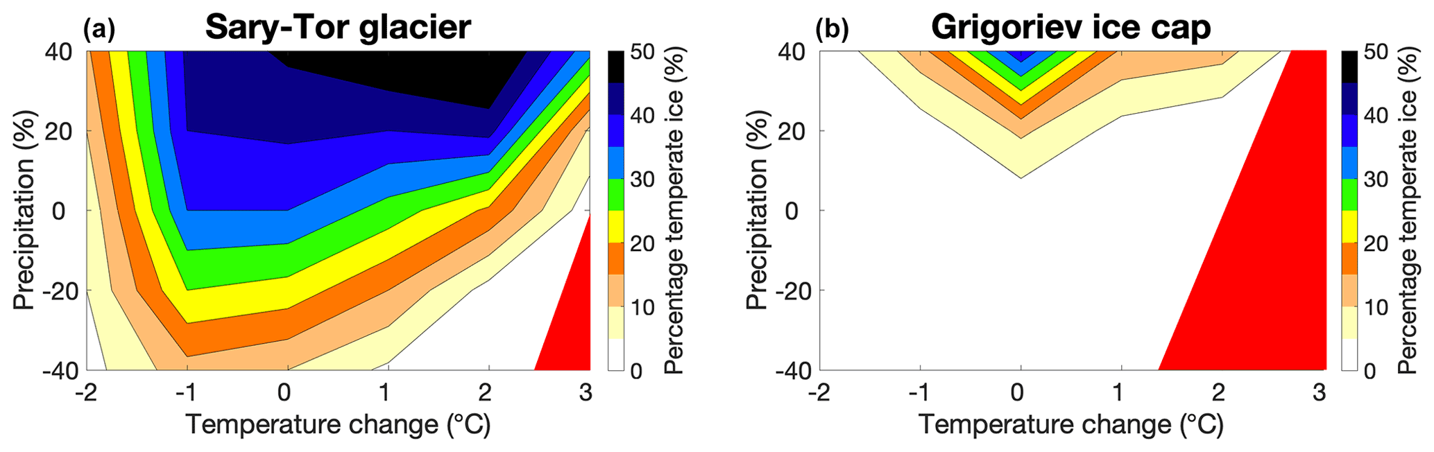
Figure 12 Fractional amount of temperate ice for different combinations of temperature and precipitation changes for the Sary-Tor glacier (a)and the Grigoriev ice cap (b). For combinations in the red area, the ice mass disappears completely.

As demonstrated, ice temperatures can vary substantially over time. Ice temperatures at higher altitudes, where melting is currently limited by the colder climate, rise more strongly than air temperatures because of the enhanced formation of refrozen water (and the associated release of latent heat) (see Sect. 4.4.2). Such a firn warming has also been observed and modelled at other glaciers (Hoelzle et al., 2011; Vincent et al., 2020; Mattea et al., 2021). Further, most climate models indicate a slight increase in winter precipitation (Sorg et al., 2012), which would imply an increase in s_max and thus a strengthening of the snow insulation effect. Evidence of a precipitation increase has been observed on Abramov glacier in the Pamir Alay (Kronenberg et al., 2021). As a result, englacial temperatures generally rise, and part of the glaciers or ice caps in the inner Tien Shan can undergo a transition from a cold to a polythermal or from a polythermal to a temperate regime (Arkhipov et al., 2004; Gusmeroli et al., 2012). Such a transition enhances ice flow and can fundamentally alter the ice dynamics (Marshall, 2021).

6 Conclusion

In this study, we investigated the thermal regime of the Grigoriev ice cap and the Sary-Tor glacier, both located in the inner Tien Shan in Kyrgyzstan (central Asia), using a time-dependent, two-dimensional surface energy mass balance model coupled to a three-dimensional, higher-order thermomechanical ice flow model. Both models were calibrated with mass balance observations and temperature measurements for different periods and elevations. After calibration with the time-dependent output from the mass balance model, a firn warming parameter of 41 ^∘C (m w.e.)⁻¹ yr⁻¹ and a snow insulation parameter of 22 ^∘C (m w.e.)⁻¹ yr⁻¹ were found. Using these parameters, the ice temperature at 10–15 m depth of the Grigoriev ice cap could be modelled with a root mean square error of 0.28 ^∘C at locations with observations. The calibrated parameters were then used to model the thermal regime of both ice masses for constant 1960–1990 climatic conditions.

The simulations revealed a polythermal structure of the Sary-Tor glacier and a cold structure of the Grigoriev ice cap, apart from a thin layer of temperate ice near the bed in the central part. The difference can be attributed to a combination of a smaller amount of maximum snow depth at the end of winter, reduced refreezing of meltwater, and lower ice flow velocities and thinner ice of the Grigoriev ice cap. As a result, the Sary-Tor glacier is characterised by basal sliding and temperate ice in the upper layers, wherein water can infiltrate through intragranular veins, while this is not the case for the Grigoriev ice cap. An extensive sensitivity analysis was performed to analyse the thermal structure for combinations of historical and future air temperature and precipitation variations. This demonstrated that the Sary-Tor glacier can always be considered a polythermal glacier since the LIA and into the future, while the Grigoriev ice cap has always been and will always be characterised by a cold structure, despite the ice being warmed in the higher parts of the ice cap when air temperatures increase. The reason for this is that at these higher temperatures, the ice cap will disappear faster than it warms up to a polythermal state.

Because the selected ice masses are typical examples of ice bodies in the inner Tien Shan, and because a detailed sensitivity analysis revealed robust results to changes in the parameters and the magnitude of the geothermal heat flux, it is reasonable to conclude that the results of this study can be generalised for similar types of glaciers and ice caps in the study area. Valley glaciers in the inner Tien Shan are probably almost all polythermal, while the high-altitude ice caps are expected to be mainly cold. Glaciers in the outer ranges, which are associated with larger amounts of precipitation, might be temperate as well. These findings are important as the dynamics of the ice masses can only be understood and modelled precisely if ice temperature is considered correctly in ice flow models. The calibrated parameters of this study can be used in applications with ice flow models for individual ice masses as well as to optimise more general models for large-scale regional simulations.