Drone-based ground-penetrating radar (GPR) application to snow hydrology

Seasonal snowpack deeply influences the distribution of meltwater among watercourses and groundwater. During rain-on-snow (ROS) events, the structure and properties of the different snow and ice layers dictate the quantity and timing of water flowing out of the snowpack, increasing the risk of flooding and ice jams. With ongoing climate change, a better understanding of the processes and internal properties influencing snowpack outflows is needed to predict the hydrological consequences of winter melting episodes and increases in the frequency of ROS events. This study develops a multi-method approach to monitor the key snowpack properties in a non-mountainous environment in a repeated and non-destructive way. Snowpack evolution during the winter of 2020–2021 was evaluated using a drone-based, ground-penetrating radar (GPR) coupled with photogrammetry surveys conducted at the Ste-Marthe experimental watershed in Quebec, Canada. Drone-based surveys were performed over a 200 m² area with a flat and a sloped section. In addition, time domain reflectometry (TDR) measurements were used to follow water flow through the snowpack and identify drivers of the changes in snowpack conditions, as observed in the drone-based surveys.

The experimental watershed is equipped with state-of-the-art automatic weather stations that, together with weekly snow pit measurements over the ablation period, served as a reference for the multi-method monitoring approach. Drone surveys conducted on a weekly basis were used to generate georeferenced snow depth, density, snow water equivalent and bulk liquid water content maps.

Despite some limitations, the results show that the combination of drone-based GPR, photogrammetric surveys and TDR is very promising for assessing the spatiotemporal evolution of the key hydrological characteristics of the snowpack. For instance, the tested method allowed for measuring marked differences in snow pack behaviour between the first and second weeks of the ablation period. A ROS event that occurred during the first week did not generate significant changes in snow pack density, liquid water content and water equivalent, while another one that happened in the second week of ablation generated changes in all three variables. After the second week of ablation, differences in density, liquid water content (LWC) and snow water equivalent (SWE) between the flat and the sloped sections of the study area were detected by the drone-based GPR measurements. Comparison between different events was made possible by the contact-free nature of the drone-based measurements.

1 Introduction

By acting as transient storage, seasonal snow cover determines the amplitude of spring floods, the level of late summer flows and the recharge of aquifers (DeWalle and Rango, 2008). Snowmelt floods are a cause of economic losses and sometimes loss of life (Ding et al., 2021), while insufficient aquifer recharge affects water availability for agricultural and industrial uses, fresh water supply, and the ecology of river systems (Dierauer et al., 2021).

Recent changes in snow cover characteristics have been reported from different regions of the globe (Magnusson et al., 2010; Zhang et al., 2015;Hodgkins and Dudley, 2006; Cho et al., 2021; Ford et al., 2021; Najafi et al., 2017). Climate change projections anticipate further alteration of snowpack characteristics: seasonal snowpack depth is expected to diminish (Dierauer et al., 2021), the winter maximum snow water equivalent to decline (Sun et al., 2019) and the spring melt to occur earlier in the season (Gergely et al., 2010). Moreover, observations and models indicate an increase in the number of winter rain-on-snow (ROS) events (Li et al., 2019). Combined with changes in snowpack characteristics, those events are predicted to trigger increases in winter flood and ice jam intensity and frequency (Morse and Turcotte, 2018; Andradóttir et al., 2021).

Within this context, monitoring the spatiotemporal evolution of snow cover properties appears essential for anticipating adverse climate change consequences on winter hydrology and groundwater recharge (Lindström et al., 2010).

• Snow depth (h), snow water equivalent (SWE), density (ρ) and liquid water content (LWC) are among the most measured properties of the snowpack (Kinar and Pomeroy, 2015). These four variables are considered key properties for characterizing the snowpack's hydrological behaviour (Vionnet et al., 2021). Different technics have been developed over time to independently monitor those four variables over very limited surfaces (less than 100 m² for most of them).

• Snow depth is widely monitored using ultrasonic sensors (Doesken et al., 2008), and methods like global navigation satellite system interferometric reflectometry (GNSS-IR) (Li et al., 2021) and terrestrial laser scanning (Prokop, 2008; Revuelto et al., 2015; Deems et al., 2017) are gaining in popularity. Still, destructive manual measurements remain extensively used for snow depth surveying (Leppänen et al., 2016).

• SWE can be calculated based on manual snow coring to estimate sample volume and mass. The manual method is time-consuming, destructive and of moderate precision (Goodison et al., 1987; Morris and Cooper, 2003; Sturm and Holmgren, 2018; Paquotte and Baraer, 2022). Automatic monitoring makes it possible to capture SWE temporal variability. The methods most often used are gamma ray monitoring (GMON), cosmic ray neutron probe (CNRP), snow pillows and plates, the system for acoustic sensing of snow (SAS2), the snowpack analyzer (SPA-2), and GNSS receiver-based SWE estimators (Yu et al., 2020). Most of those technics require site calibration.

• Snow density is commonly measured through gravimetric measurements or calculated from snow depth and SWE measurements (Conger and McClung, 2009). In dry conditions, snow density can be estimated with a dielectric permittivity measurement system such as the Finnish Snow Fork (Hao et al., 2021). Other methods include neutron probes (Hawley et al., 2008) and diffuse near-infrared transmission (Gergely et al., 2010).

• The most common in situ LWC measurement methods are based on snow permittivity measurements. The Snow Fork (Sihvola and Tiuri, 1986), the Denoth device (Denoth, 1995) and the A2 Photonic WISe sensor (Webb et al., 2021) are among the most popular devices to measure LWC. They all have an accuracy level of around 1 % of the volumetric LWC. The most accurate method, however, which is often used as a reference for those devices, is freezing or melting calorimetry (Webb et al., 2021; Mavrovic et al., 2020). LWC may be monitored unattended using time domain reflectometry (TDR), but multiday monitoring using that technique still presents a challenge (Lundberg et al., 2016).

Even if they are accurate in following the evolution of each variable in time, those techniques do not allow for capturing the spatial variability in the snowpack properties unless they are repeated at a multitude of points. Aerial and spaceborne remote sensing represents an attractive alternative for that purpose.

With a vertical accuracy of less than 10 cm, airborne photogrammetry allows for a non-destructive monitoring of the spatial variability in snow depth in open areas (Bühler et al., 2016a; Avanzi et al., 2018; Harder et al., 2020; Jacobs et al., 2021). In forested areas, airborne lidar (light detection and ranging) has proven a more accurate option (Koutantou et al., 2021; Dharmadasa et al., 2022). The use of satellite-based remote sensing for snow depth and, by extension, SWE mapping has received much attention over the past decade (Guneriussen et al., 2001; Rott et al., 2003). While showing promising results and fast improvements in large open areas of a range of several square kilometres (e.g. McGrath et al., 2019), satellite-based SWE and/or snow depth estimations still involve coarse spatial data with a high degree of uncertainty when passive sensors are used (Mortimer et al., 2020), and some accuracy challenges still exist with active sensors (Pfaffhuber et al., 2017). This is the case in mountainous areas, for example (LiYun Dai, 2022).

From the 1980s onward, the use of ground-penetrating radar (GPR) has been seen as a solution to overcome the difficulties in capturing key properties of and spatial variability in the snow pack, as described above (Marchand et al., 2003). First carried by the operator, GPR airborne and ground-vehicle-based applications have risen in popularity due to their abilities to cover transects that are 1/10 of a kilometre long (Bruland and Sand, 1998). Radargrams generated using GPR show the influence a milieu has on the emitted electromagnetic wave that travels through it. This influence is characterized by the milieu's permittivity, expressed as a complex number. For snow layers, the real component of the permittivity is mostly a function of snow density, snow depth and LWC. As SWE can be calculated from snow depth and density, GPR therefore allows for measuring a physical characteristic that is related to the four key snowpack properties in a single survey (Di Paolo et al., 2018).

Since the 1980s, GPR has been shown to be a valuable tool for measuring physical snowpack characteristics (Holbrook et al., 2016). It is one of the most-used methods in snowpack studies (Vergnano et al., 2022), and the spatial variability in snow properties has been extensively assessed using GPR (Lundberg et al., 2010; Previati et al., 2011; Holbrook et al., 2016).

However, GPR applications in monitoring one or several of the four key snowpack characteristics still involve different challenges, such as the following.

• The real component of the permittivity requires the snow depth to be known or estimated (Di Paolo et al., 2020).

• Different empirical equations have been developed to relate snow density and LWC to the real component of the permittivity (Frolov and Macheret, 1999; Di Paolo et al., 2018). In dry conditions, LWC being neglectable, a direct relation exists between the snow density and the relative permittivity. On the other hand, the introduction of liquid water into the snowpack cannot be accurately characterized with GPR velocity alone (Bradford and Harper, 2006). In the absence of other measurements allowing for mapping of LWC or snow density in wet conditions, either an assumption needs to be made regarding snow density variability from spot measurements (e.g., Webb et al., 2020; Yildiz et al., 2021) or an empirical relation must be parametrized by calibration (e.g. Singh et al., 2017).

• Ground-based GPR applications require direct contact with the snow surface, modifying its properties (Valence and Baraer, 2021) and making subsequent surveys not fully representative of natural conditions.

• Air surveys such as the helicopter-based ones are limited by high operating costs, while ground-based surveys are difficult to conduct on unstable and steep slopes (Vergnano et al., 2022).

Recent developments show interesting potential to overcome those challenges. Combining GPR applications with other measurements has been shown to be an efficient way to overcome the first two challenges. For instance, Marchuk and Grigoryevsky (2021) improved GPR-based snow depth profiling by associating GPR to a laser range finder. The use of drone-based surface mapping methods such as photogrammetry or lidar in snowpack studies provides reliable snow depth maps (Bühler et al., 2016b). Lundberg et al. (2016) and Yildiz et al. (2021) used drone-based photogrammetry or lidar to integrate snow depth measurements into SWE calculations. Combining techniques that monitor the temporal evolution of the snow permittivity, such as TDR, with GPR has been shown to be a promising approach to studying snowpack spatial variability over a given period (Godio et al., 2018). Estimating LWC from frequency-dependent attenuation of the GPR signal, as proposed by Bradford et al. (2009), is another way to address the wet snowpack characterization issues.

Actual developments in drone-borne GPR have opened new avenues in GPR-based snow pack studies (Francke and Dobrovolskiy, 2021). Recent studies have shown it to be valuable in snow avalanche applications (McCormack and Vaa, 2019) and in snow depth mapping (Tan et al., 2017; Vergnano et al., 2022). Similarly, drone-based ultra-wide-band (Jenssen and Jacobsen, 2020) and software-defined radar (Prager et al., 2022) applications to snowpack characterization surveys have recently been demonstrated to be potentially ground-breaking solutions.

The present study aimed to monitor the spatiotemporal variability in snow depth, snow density, SWE and snow LWC of a snowpack over flat and sloped areas with a non-destructive approach. This objective was achieved by combining some of the emerging solutions described above with more traditional snow-monitoring techniques in a novel way. This combination included drone-based photogrammetry, drone-based GPR, and continuous monitoring of SWE, snow depth and snow permittivity using TDR and snow-pit-based measurements.

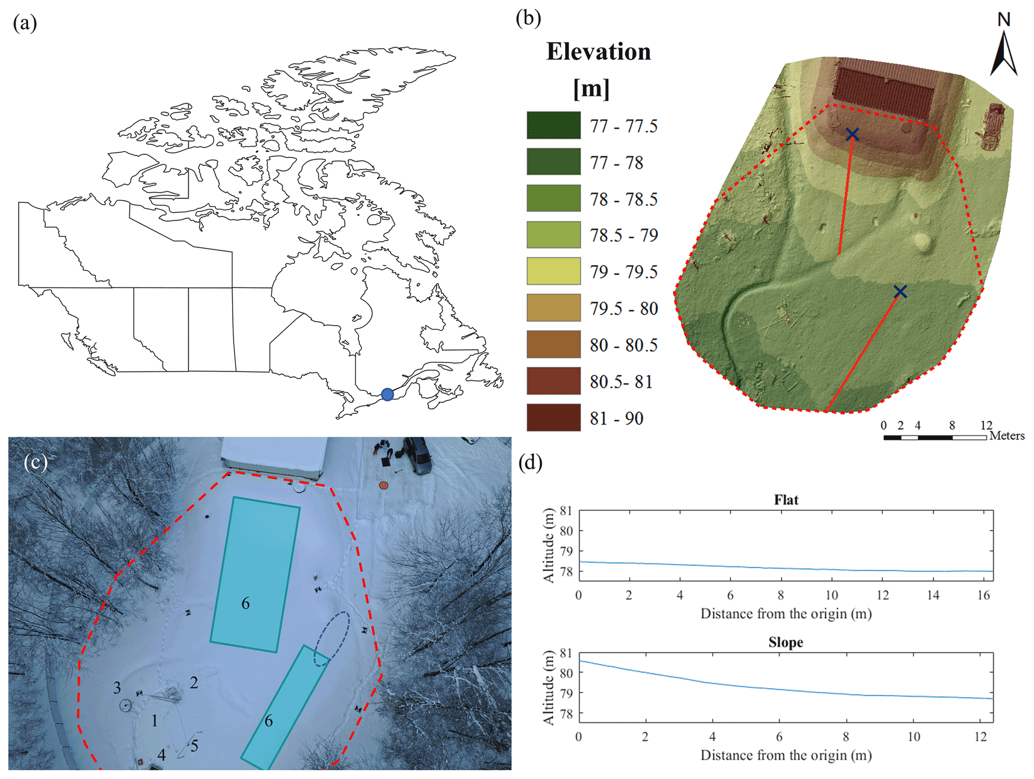
Figure 1 Study site. (a) Location of the BVE of Ste-Marthe. (b) Snow-free DSM of the main station area; the red polygon delimits the study area, red lines represent the two studied transects, and blue crosses mark the two profiles' origins. (c) Overview of the BVE of Ste-Marthe main station; the red polygon delimits the study area, blue areas represent the two studied areas, and dashed dark blue ellipses represent the zone used for the snow pit. Numbers identify devices of interest for the present study: (1) sonic sensor, (2) ground and snow temperature sensors, (3) shielded precipitation gauge, (4) snow lysimeter, (5) SWE sensor, and (6) TDR instruments. (d) Altitude profile of the two studied transects.

2 Study site

The study was conducted at the bassin versant experimental (BVE) of Ste-Marthe, an experimental watershed located approximately 70 km west of Montréal, in Quebec, Canada (45.4239^∘ N, 74.2840^∘ W) (Fig. 1a). The main station of the BVE of Ste-Marthe is situated at 120 m above sea level in an approximately 200 m² forest clearing (Fig. 1b and c). A distinction is made between two different topographic areas of the clearing: one of approximately 30 m², categorized as flat, and the other of approximately 50 m², categorized as sloped (Fig. 1d). The automatic weather station (AWS) measures various hydroclimatic variables. Those of interest for the purpose of this study are listed in Table 1.

Table 1 List of the instruments used in this study. Accuracy is either given by the manufacturer or estimated for worst-case scenarios. Adapted from Paquotte and Baraer (2022).

Measurements took place during the winter of 2020–2021, from 26 February to 26 March. Two rain-on-snow (ROS) events occurred during this period. The first ROS was observed from 28 February to 1 March and the second from 9 to 12 March.

Field visits for drone-based surveys and snow pit measurements occurred on 26 February, 5 March, 12 March and 19 March. 26 February corresponded to the end of the accumulation period, while the ablation period started on 27 February.

Table 2 Methods combined in this study and classified based on the sampling frequency and the spatial coverage.

3 Methods

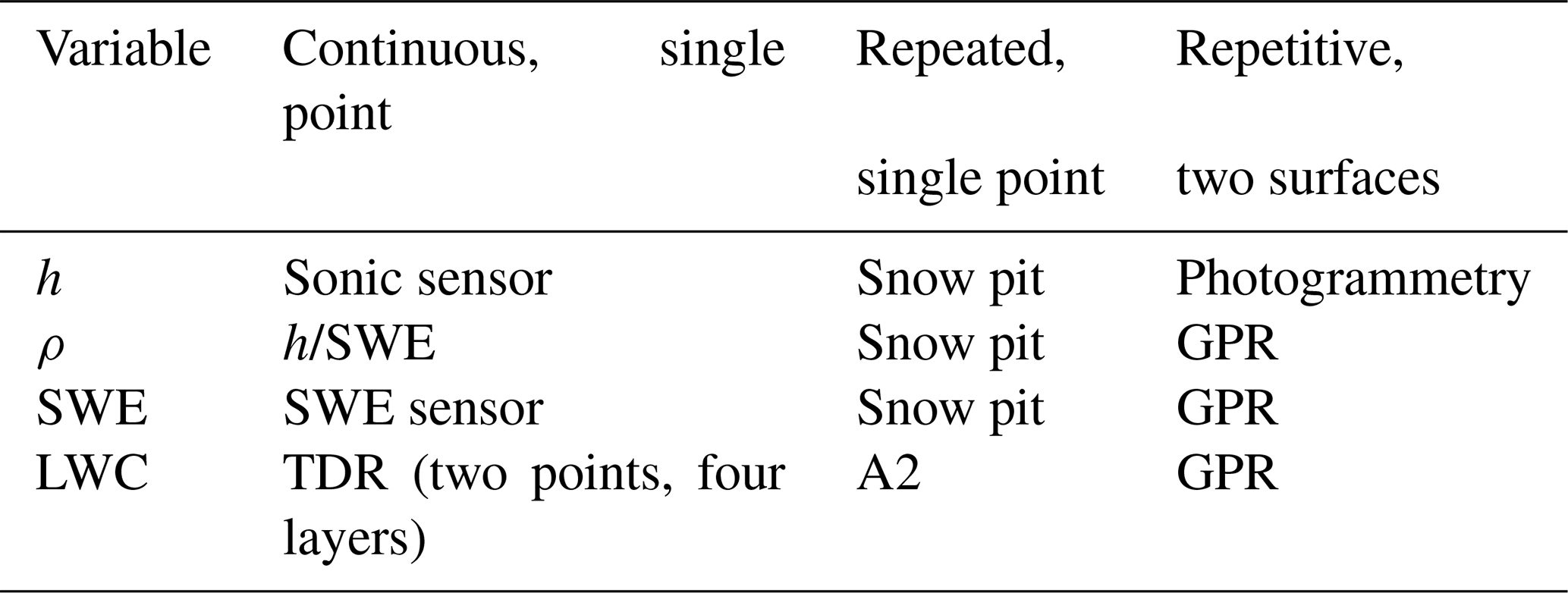
The spatiotemporal variability of snow depth, snow density, SWE and snow LWC was assessed by combining different methods with different sampling approaches. Table 2 provides a list of the different methods that were used. Those were split into three categories according to the frequency of measurements and the spatial coverage. Repeated surveys conducted over the flat and sloped areas were used to produce maps of the four studied variables on a weekly basis. Continuous and repeated measurements at a single point were used for verification of the map data at a given point in the study area. TDR sensors were an exception: a total of eight probes were split between the two areas. At each spot, probes were placed on different hard layers on the snowpack. These layers were identified as possible vectors for lateral flow (Evans et al., 2016).

3.1 AWS monitoring

Data from the AWS were recorded using a Campbell Scientific CR1000 data logger. AWS sensors included the snow lysimeter situated at less than 10 m from the surveyed flat area and presented a comparable exposition to sunlight.

Therefore, it was expected that both snow depth records would exhibit comparable results. The snow's relative density was calculated using the snow depth and the SWE measurements, following Eq. (1):

$$\begin{array}{}\text{(1)}& \mathrm{SWE}=h\times \mathit{\rho }.\end{array}$$

SWE and h are both in metres, and ρ is dimensionless.

The frozen ground depth was estimated by interpolation of ground temperatures measured from 10 to 60 cm below the ground level at 10 cm depth intervals. Snowpack temperature was measured with four thermometers at 0, 10, 20 and 30 cm above the ground level. To avoid using snowpack temperature measurements that could have been influenced by solar radiation or by contact with air, snowpack temperature measurements were not considered after 17 March 2021, the day the snow height decreased below 40 cm above ground level.

3.2 Manual measurements

Manual measurements were conducted on a weekly basis, on the same days as the drone surveys. Snow pits were excavated, with northern orientations, at approximately 75 cm from the previous ones, following the method presented by Fierz et al. (2009). The snow pits were located less than 3 m from the flat area surveyed by drone and presented a comparable exposition to sunlight. For each pit, layer identification was followed by sequential depth, density and snow temperature measurements. Each layer was isolated from the preceding one using a thin metallic plate and sampled using a metallic cylinder of 0.3 dm² or a cylindrical plexiglass sampler with a surface of 0.5 dm². The sample mass was measured in situ with a scale of ±1 g accuracy.

LWC measurements were made in the snow pit using an A2 Photonic WISe sensor. Two vertical measurement profiles with 10 cm intervals between observations were created for each snow pit. Even if the manufacturer's device precision was ±1 % of LWC, we anticipated a higher degree of uncertainty, as measurement through ice layers was not possible.

Snow pack total depth and bulk SWE were calculated by adding up the individual layer values for these measures. Bulk relative density and LWC were calculated by taking the weighted mean of the measurements of a layer's thickness.

3.3 TDR monitoring

The CS610 probes were controlled using a TDR200 (both from Campbell Scientific). Each probe was bench calibrated according to the Campbell Scientific guidelines before deployment. On-site, each CS610 was inserted into the snow and left lying over a hard layer without any guide or support. This setup was chosen to allow the probe to move downward together with the supporting hard layer as the snowpack settled. Maintaining probes at a fixed position above the ground triggers air pocket formation around the metallic rod over time, affecting the measurements' accuracy (Pérez Díaz et al., 2017). As no visible differences in stratigraphy were observed between the flat and sloped areas over the accumulation period, hard layers supporting the probes were identified the same way.

• α represents the ground level. Probes were installed on January 8 in the flat area and 26 January at the base of the slope. At both locations, the snow layer on top of the ground was unconsolidated and heterogeneous.

• β is a wind crust formed on 30–31 December. Probes were installed on the same days as the ones on layer α. The layer β was overlaid by unconsolidated granular snow.

• γ is a hard settled snow layer that formed on 15 January. Probes were installed on 26 January. At that time, the hard snow layer was overlaid by a thin layer of fresh snow.

• ε is an ice layer that formed after a freezing rain event which occurred on 16 February. Probes were installed on top of that layer on 22 February at both locations.

TDR probes measure the relative permittivity of the surrounding material. In snow, the relative permittivity is a function of the density and the liquid water content mainly (Stacheder et al., 2009). Placed at different spots, initial relative permittivity values measured by the probes naturally differ slightly from each other. In order to allow comparison of the permittivity evolution between two probes placed over the same layer, relative permittivity values were normalized by dividing all values measured by a TDR probe by the first measurements made after installation of that given probe value. Doing so allowed the researchers to start each TDR-derived time series from 1. With a 15 min measurement interval, it was assumed that any sensible variations in permittivity (higher than 10 % of the initial value) between two successive measurements were due to changes in liquid water content, as such changes would occur over a longer timescale if due to a change in snowpack density only (Stacheder et al., 2005).

3.4 Drone-based photogrammetry

A DJI Mavic 2 Pro drone was used to capture the RGB images used for photogrammetry. During a flight time of approximately 20 min, the drone took around 200 images with an 80 % overlap at an elevation of 25 m above ground level. The Mavic 2 Pro is equipped with a TOPODRONE global navigation satellite system (GNSS) to allow post-processing kinematic (PPK) treatment to correct images' locations. The uncertainty claimed by the manufacturer is 3–5 cm in all directions. PPK corrections were made using a Reach RS2 GNSS base station, with a manufacturer's uncertainty of 4 mm in the horizontal direction and 8 mm in the vertical. After each site visit, collected images were processed using the Pix4Dmapper software to produce digital surface models (DSMs). The expected horizontal resolution is 0.6 cm per pixel. Vertical accuracy was assessed using ground control points (GCPs). For each survey, 10 GCPs were disposed all around the study area; GCPs were placed approximately at the same position for each survey. Control points were geo-localized using a KlauGeomatic 7700B GNSS rover, ensuring a 5 cm accuracy. Comparing the uncorrected DSMs produced by photogrammetry to the DSMs after correction using control points showed variations under 3 cm in all three directions, which is within the expected accuracy of the KlauGeomatic GNSS. The use of control points did not lead to meaningful improvements of the map georeferencing, validating the accuracy of maps produced using PPK adjustments only.

Finally, snow depth maps were produced by subtracting a snow-free DSM produced on 6 April, just after the complete thaw of the snow cover and just before the vegetation growth, from the DSM produced in winter conditions. This was done using the Esri Geographic Information System (GIS) software ArcGIS, following the protocol presented by Bühler et al. (2016a) and Yildiz et al. (2021).

3.5 Drone-based GPR permittivity measurement

GPR surveys were performed using a Radar Systems Inc. Zond 1.5 GHz carried by a DJI Matrice (M) 600 Pro drone. The GPR integration system and the flight control software (UgCS) were supplied by SPH Engineering. Maximizing GPR measurements requires flying at 1.2 m s⁻¹ and at approximately 1 m above the surveyed surface. Drone altitude was controlled using a terrain-following system supplied by SPH Engineering. The system is made of the UgCS SkyHub onboard computer coupled with a radar altimeter. The onboard computer manages the power supply and the GPR data. The M600 Pro was equipped with a KlauGeomatic 7700B GNSS allowing position correction via PPK. Similar to the photogrammetry, PPK corrections were made using the Reach RS2 GNSS as a base station. GPR data were referenced by post-treatment using the KlauGeomatic PPK solution. Surveys were performed over both the flat and sloped areas. Post-treatment of radargrams was performed with the Radar System Inc. Prism2 software. The GPR system was sampled every 512 ns over both flat and sloped areas, and the drone's flight followed north–south transects. Thus, the spatial resolution of GPR measurements was a function of the actual drone speed (different from expected drone speed due to wind and other meteorological conditions affecting the drone flight) and the sampling frequency. For each survey, six transects on the flat area and nine transects on the slope were surveyed. The distance between two consecutive transects was 50 ± 20 cm. Post-treatment consisted of applying a background removal filter, adjusting the gain, and applying a time-delay compensation. The ground–snow and snow–air interfaces were detected automatically wherever possible and manually where the layer boundaries were not recognized by the automatic graphic interpretation tool. Figure 2 provides two examples of radargrams with identified layer boundaries. Given that GPR measurements were geo-localized using the same PPK as the photogrammetry, the radargram georeferencing was considered to have a 5 cm accuracy.

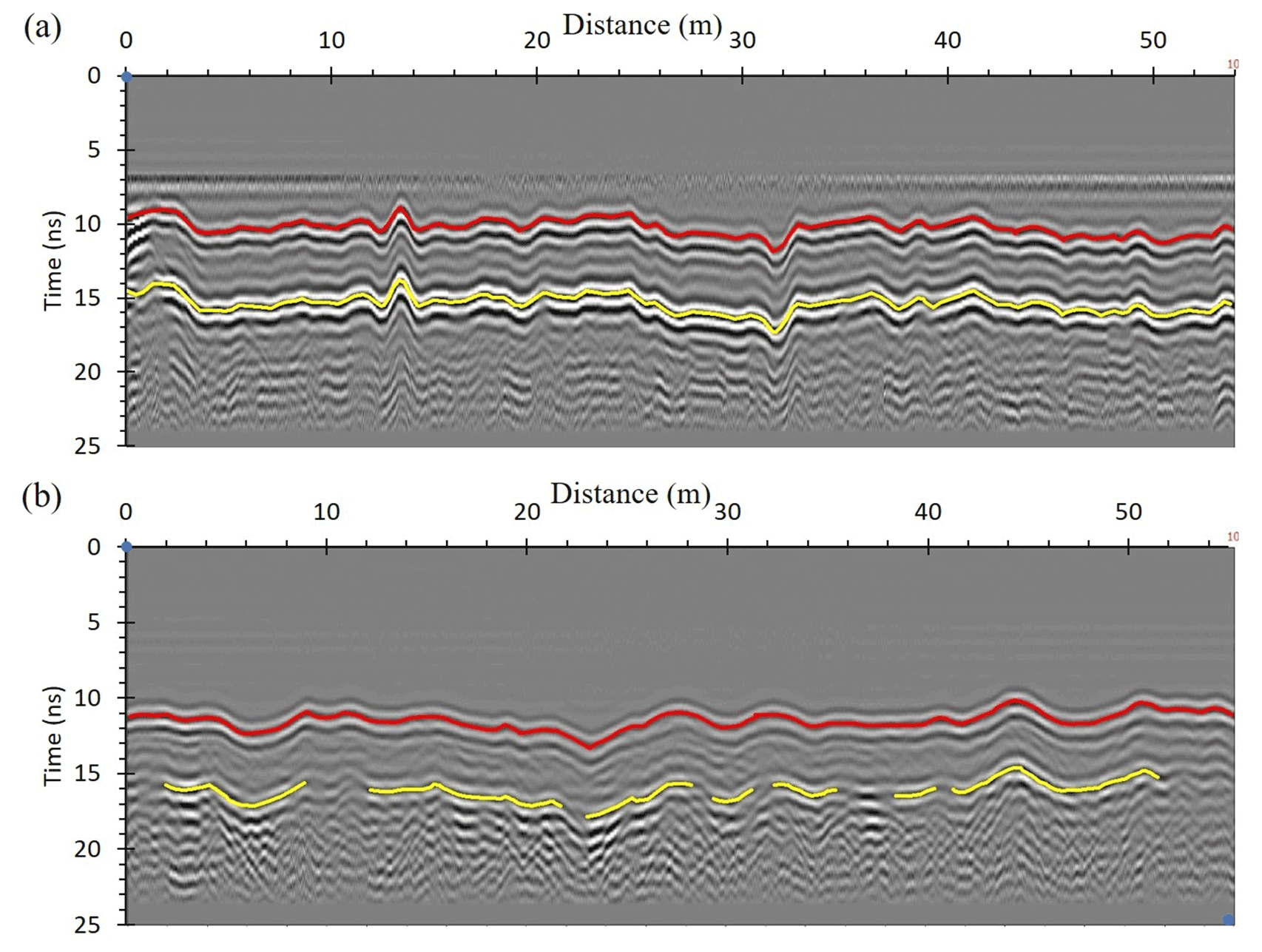
Figure 2 Flat-area drone-based 1.5 GHz GPR radargrams collected on (a) 5 March and (b) 12 March (considered as the less legible radargrams). The red line represents the air–snow interface, and the yellow line represents the snow–ground interface.

Snow depth for each GPR transect was extracted from the snow depth maps produced by photogrammetry using ArcGIS. The velocity of the electromagnetic wave within the snowpack (ν) and the snow height (h) extracted from the DSM are related as follows:

$$\begin{array}{}\text{(2)}& \mathit{\nu }={\displaystyle \frac{h}{\mathrm{TWT}/\mathrm{2}}},\end{array}$$

where TWT is the two-way travel time of the wave within the snowpack (in ns). TWT is extracted from the radargrams by taking the difference between the air–snow interface and snow–ground interface two-way travel times.

The relative permittivity of the snowpack is a complex number. Its real part (${\mathit{\epsilon }}_{\mathrm{s}}^{\prime }$) is calculated using Neal (2004):

$$\begin{array}{}\text{(3)}& {\mathit{\epsilon }}_{\mathrm{s}}^{\prime }={\left(c/v\right)}^{\mathrm{2}},\end{array}$$

where c stands for the velocity of light in a vacuum (taken as equal to 0.3 m ns⁻¹).

3.6 Drone-based GPR frequency-dependent attenuation analysis

In wet conditions, the imaginary part of the permittivity of the snow (${\mathit{\epsilon }}_{\mathrm{s}}^{\prime \prime }$) is estimated using the GPR frequency-dependent attenuation analysis method proposed by Bradford et al. (2009). In the standard GPR frequency range (10 MHz–1 GHz), ${\mathit{\epsilon }}_{\mathrm{s}}^{\prime }$ is strongly dependent on LWC and assumed to be independent of frequency. Assuming that the frequency-dependent attenuation of an electromagnetic wave through water is linearly related to frequency (Turner and Siggins, 1994), the attenuation coefficient over the GPR signal band can be written as

$$\begin{array}{}\text{(4)}& \mathit{\alpha }={\mathit{\alpha }}_{\mathrm{0}}+{\displaystyle \frac{\sqrt{{\mathit{\mu }}_{\mathrm{0}}{\mathit{\epsilon }}_{\mathrm{s}}^{\prime }}}{\mathrm{2}{Q}^{\ast }}}\mathit{\omega },\end{array}$$

where Q^∗ represents the generalization of the attenuation quality parameter in the linear region of the attenuation, ∝₀ the impact of low frequencies in the radar attenuation, ω the angular frequency and μ₀ the permeability in the free space.

Within the frequency range of 1 to 1500 MHz, Q^∗ is assumed to be constant (Bradford et al., 2009) and related to ${\mathit{\epsilon }}_{\mathrm{s}}^{\prime \prime }$ as follows:

$$\begin{array}{}\text{(5)}& Q^{\ast }={\displaystyle \frac{{\mathit{\epsilon }}_{\mathrm{s}}^{\prime }}{\mathrm{2}{\mathit{\epsilon }}_{\mathrm{s}}^{\prime \prime }}},\end{array}$$

where a GPR generates waves in the form of a Ricker wavelet, the frequency f₀ of the spectral maximum of the GPR wave, measured at the snow–air interface on the radargram, and the frequency f_t of the spectral maximum, measured at the ground–snow interface, which are related to Q^* (Bradford, 2007):

$$\begin{array}{}\text{(6)}& \left\{\begin{array}{l}\frac{\mathrm{1}}{Q^{\ast }}=\frac{\mathrm{4}}{\mathrm{TWT}}\frac{{\mathit{\omega }}_{\mathrm{0}}^{\mathrm{2}}-{\mathit{\omega }}_t^{\mathrm{2}}}{{\mathit{\omega }}_{\mathrm{0}}^{\mathrm{2}}{\mathit{\omega }}_t}\\ {\mathit{\omega }}_{\mathrm{0}}=\mathrm{2}\mathit{\pi }{f}_{\mathrm{0}}\\ {\mathit{\omega }}_t=\mathrm{2}\mathit{\pi }{f}_t\end{array}\right..\end{array}$$

In the present study, f₀ and f_t were measured by randomly sampling at least 10 points on each GPR line. For each selected point, readings were made on five consecutive traces using the Prism2 software. Peak frequencies for each point were calculated by taking the median of the measurements. When at least one trace showed a higher frequency at the ground–snow interface than at the snow–air interface, two extra traces were used; ${\mathit{\epsilon }}_{\mathrm{s}}^{\prime \prime }$ was then computed using Eqs. (5) and (6), with ${\mathit{\epsilon }}_{\mathrm{s}}^{\prime }$ being calculated using Eqs. (2) and (3).

LWC and the relative density of dry snow (ρ_d) were then calculated with the following set of dimensionless empirical equations proposed by Tiuri et al. (1984) and Sihvola and Tiuri (1986):

$$\begin{array}{}\text{(7)}& {\displaystyle }{\mathit{\epsilon }}_{\mathrm{d}}^{\prime }=(\mathrm{1}+\mathrm{1.7}{\mathit{\rho }}_{\mathrm{d}}+\mathrm{0.7}{\mathit{\rho }}_{\mathrm{d}}^{\mathrm{2}}),\text{(8)}& {\displaystyle }{\mathit{\epsilon }}_{\mathrm{s}}^{\prime }=\left(\mathrm{0.1}\mathrm{LWC}+\mathrm{0.8}{\mathrm{LWC}}^{\mathrm{2}}\right){\mathit{\epsilon }}_{\mathrm{w}}^{\prime }+{\mathit{\epsilon }}_{\mathrm{d}}^{\prime },\text{(9)}& {\displaystyle }{\mathit{\epsilon }}_{\mathrm{s}}^{\prime \prime }=\left(\mathrm{0.1}\mathrm{LWC}+\mathrm{0.8}{\mathrm{LWC}}^{\mathrm{2}}\right){\mathit{\epsilon }}_{\mathrm{w}}^{\prime \prime },\end{array}$$

where ε_d' is the bulk permittivity of dry snow, and ${\mathit{\epsilon }}_{\mathrm{w}}^{\prime }$ and ${\mathit{\epsilon }}_{\mathrm{w}}^{\prime \prime }$ are the real and the imaginary parts of the relative permittivity of pure water, respectively.

Equations (7), (8) and (9) were established for a measurement frequency of 1 GHz and were assumed to remain valid for the purpose of the present study.

The relative snow density (ρ) was then calculated with the following equation:

$$\begin{array}{}\text{(10)}& \mathit{\rho }={\mathit{\rho }}_{\mathrm{d}}+\mathrm{LWC}.\end{array}$$

Finally, the SWE was calculated using the relative density (ρ) calculated using Eq. (10) and with the snow depth (h) extracted from the DSM produced by photogrammetry using Eq. (1). LWC maps were then produced by extrapolating the punctual results to area values using an inverse distance weighting interpolation with barriers set at 2 m. For each LWC map, 10 ± 2 points per transect were randomly selected for the interpolation. The inverse distance exponent was set at two, the maximum distance for data calculation was set at 2 m, and the minimum number of points considered in the calculation was three. The interpolation was used to create LWC maps of 5 cm cell size.

For the surveys on 26 February and 5 March, the snowpack was assumed to be dry, as the surveys were preceded by several cold days and as the snowpack temperatures measured were all below 0 ^∘C. The SWE was determined using the assumptions that ${\mathit{\epsilon }}_{\mathrm{d}}^{\prime }={\mathit{\epsilon }}_{\mathrm{s}}$', ρ_s=ρ_d, and LWC = 0.

For the surveys on 12 and 19 March, the SWE was determined following the GPR attenuation method.

Figure 3 AWS measurements during the winter 2022 ablation period. (a) Air temperature and precipitations; (b) frost depth and lysimeter outflow; (c) snow temperature at four different heights; (d) snow water equivalent, snow height and relative snow density. Variables associated with the different line colours are indicated in each panel. Semi-transparent grey shadings represent mild episodes. Mild episode identification is given underneath panel (a). Details about variable descriptions and measurements are given in Table 1. Vertical dashed lines indicate field measurements days.

4 Results

4.1 AWS

Figure 3 presents the AWS-relevant measurements over the study period. The 27 February measured snowpack temperatures were all below 0 ^∘C and had not been altered by any significant ROS or major melt event yet.

Between 27 February and 1 March, the snowpack was affected by a first mild episode (M.E. 1) that ended with a ROS event. Mild episodes are here defined as more than 24 h long periods with continuous above-zero air temperatures. The first week of investigation was also characterized by several snow precipitation events. The ROS event lasted 45 min, with 1.6 mm of cumulative precipitations during the first 30 min and only 0.1 mm in the last 15 min. M.E. 1 warmed up the snowpack to nearly 0 ^∘C at all measured depths, generated slightly more than 1 mm of cumulative outflow at the base of the snowpack, and increased both the SWE and relative snow density by 15 mm equivalent and 0.05, respectively. Outflow at the snowpack's base started while the measured snowpack temperatures were still negative, suggesting that at least part of the outflow was made of liquid precipitation flowing through the snowpack. M.E. 1 was followed by a drop in air temperature of 25 ^∘C, starting the beginning of a 7 d long cold period. Over that cold period, the measured snowpack temperatures dropped below 0 ^∘C, while SWE and relative snow density stabilized. Outflow at the snowpack's base stopped 24 h after the temperature started to decrease. Considering that during this mild episode at least part of the ground remained frozen, with negative temperatures observed between 0 and −30 cm under the soil surface, it is assumed that no significant ground infiltration occurred during M.E. 1 (Dingman, 1975). This suggests that most of the rain percolation either froze inside the snowpack or flowed longitudinally at its base.

The second survey occurred on 5 March, during the 7 d long cold period described here above, over a dry snowpack.

A second mild episode (M.E. 2) started on 8 March and ended on 12 March, the day of the third survey. On 11 March, the air temperature reached a maximum of 15 ^∘C, and a ROS event occurred. It took 2 d for the warm conditions to warm the snowpack up to 0 ^∘C at all measurement points and to generate outflow at the snowpack's base. The second ROS event occurred on an already warm snowpack and produced 0.8 mm of precipitation over 30 min. This ROS event was therefore slightly less intense than the first one. The snow lysimeter measured a cumulative outflow comparable to that during M.E. 1. As the soil remained frozen during this second mild episode, most of the water coming from the melt and from the precipitation was expected to have flowed horizontally at the base of the snowpack.

12 March marked the last day of M.E. 2 with air temperatures falling under 0 ^∘C. Between 8 and 12 March, snow depth decreased by almost 30 %, while SWE remained almost unchanged despite substantial liquid precipitations being recorded. Snowpack temperatures and outflow measurements indicated that at least some of the snowpack layers were wet at the time of the survey. From 12 March, air temperatures remained negative until 17 March. A refreezing front slowly moved down the snowpack, and the outflows stopped over that period, suggesting a gradual drying of the snowpack. From 17 to 18 March, a third mild episode (M.E. 3) brought the snowpack temperatures back to the melting point. An outflow of minor amplitude compared to those observed during the first two mild episodes was measured on 18 March only.

During the 19 March survey, the air temperature reached a maximum of −2 ^∘C. At that date, the snowpack was drying, with an almost continuous increase in snow density and a decreasing snowpack depth. These reached 0.48 and 38 cm, respectively.

Figure 4 Snow depth calculated by photogrammetry for the four dates covered in this study.

4.2 Drone-based photogrammetry

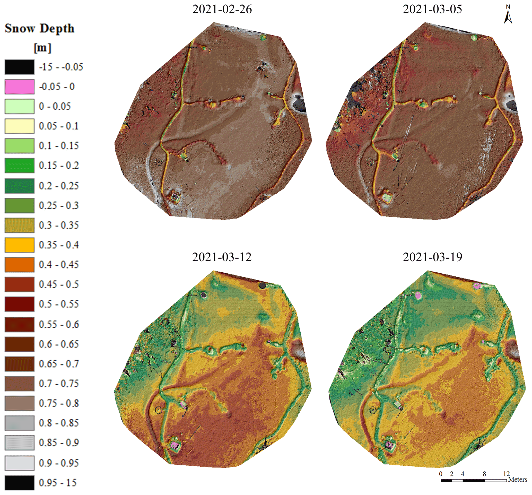
Snow cover maps produced using drone-based photogrammetry are presented in Fig. 4. On top of the uncertainty estimation described above, the maps are fully consistent with field observations. The quality of the DSM allows for identifying specific features such as trails used to access different features of the study area (e.g., lines in yellow on the 26 February 2020 map). Those trails show lower than pristine snow depths in a consistent way. Similarly, extra snow accumulation in drainage ditches (e.g., brown area in the bottom left area of the 19 March 2020 map) is well marked and consistently apparent on the different sub-figures. Overall, the snow depth maps are considered to have satisfactory accuracy for the purpose of the study.

By comparing the different Fig. 4 maps, we can observe that the snow depth decrease that occurred between 26 February and 5 March is homogeneous over the entire area, with no differences between the flat and sloped areas being visually noticeable. Snow depth in both areas on 26 February ranged between 60 and 90 cm, while on 5 March, the snow depth ranged from 50 to 80 cm in both sloped and flat areas. The situation is different when comparing the 12 March map to these first two dates. On 12 March, flat-area snow depth ranged from 35 to 55 cm, whereas the sloped-area snow depth was between 25 and 50 cm. The severe ablation and/or settling that affected the study area impacted the sloped area more than the flat one. Changes in snow depth were less pronounced between 12 and 19 March than for the previous periods. Maximum snow depth in the flat area decreased from 55 to 50 cm and from 50 to 45 cm in the sloped area between 12 and 19 March. Between 5 and 12 March, the maximum snow depth in the flat area decreased by 25 cm and by 30 cm in the sloped area.

Overall, Fig. 4 shows that the sloped and flat sections had comparable snow depths at the end of the accumulation period but reacted differently to ablation, with a faster loss of depth in the sloped area than in the flat one.

Figure 5 Normalized permittivity measured by TDR probes in the sloped (black line) and flat sections (orange line). Probe positions in each graph are shown in drawings representing a simplified description of the snowpack, with layer identification letters: (a) layer ε, (b) layer γ, (c) layer β and (d) layer α. Semi-transparent grey shadings represent mild episodes. Mild episodes are identified in panel (a). Vertical dashed lines mark field visit dates.

4.3 TDR monitoring

Relative permittivity measured using TDR probes and normalized to the value measured on 26 February at 12:30 EST are presented in Fig. 5. As described in the Methods section, rapid variations in relative permittivity are associated with a change in LWC. Given that an increase of more than 0.1 in normalized permittivity in 15 min can be considered as due to a change in LWC, the normalized relative permittivity is here used to assess the snowpack response to mild episodes in terms of water content and flow-through dynamics.

M.E. 1. The first reaction to the M.E. 1 in terms of LWC was observed on top of the layer ε (Fig. 5a). That increase in LWC led to an increase in normalized relative permittivity of 0.2 on 27 February, the day after M.E. 1 began. Snowpack response to the February 28 ROS event occurred first at the bottom of the sloped area, as suggested by the increase of 1.2 of normalized relative permittivity over the α slope layer (Fig. 4d), followed by an increase of 0.2 measured by the other TRD sensors. The detection of an increase in LWC at the base of the flat area occurred half a day after the increase for the sloped area, with an increase of about 0.7 of the normalized permittivity above both flat and sloped α layers, at a time when the air temperature had already dropped below zero. Interestingly, the lysimeter measured an outflow at the base of the snowpack in the flat area 24 h before any moisture increase was detected by the TDR probe placed on the ground in the flat area. Differences observed in timing and amplitudes at the different probe locations suggest that liquid water flows followed preferential pathways. Past that time, normalized permittivity steadily decreased in all spots, reaching a plateau representative of the new dry densities of the snow layers. The relative permittivity of the new plateau was 10 % higher than on 26 February, suggesting a slight increase in density.

M.E. 2. As was the case at the M.E. 1, the increase in normalizer relative permittivity was first observed at the base of the sloped area. The increase was followed by an increase at the other probes 24 h later, those above the β and γ layers being of very low amplitude: 0.1 to 0.2 of normalized permittivity. The strongest increase in LWC was measured over the sloped ground layer (Fig. 4d), with a normalized relative permittivity 4 times higher than the one measured on 26 February. At the end of 10 March, three of the four probed layers showed an increase in LWC, which was more pronounced in the sloped area than in the flat area. After 10 March, the fluctuation of LWC above the γ layers in the sloped area (Fig. 4c) started to mimic the one above the ground but with a lower amplitude. This synchronism suggests that the sloped area's preferential pathway flow-through mode started weakening.

M.E. 3. The sloped area showed a faster and more intense response to M.E. 3 starting on 17 March than the flat area. Unlike the flat area, the slope's LWC fluctuation started exhibiting a strong diurnal pattern, whose peak occurred a couple of hours before the peak in air temperature and the peak in lysimeter outflow.

Overall, the TDR probes showed a faster and more intense response to air temperature warming episodes on the slope compared to the flat area, the presence of preferential pathways (particularly at the start of the ablation period), and a noticeably higher influence of solar radiation on the ablation of the sloped area compared to the flat one at the end of the study period.

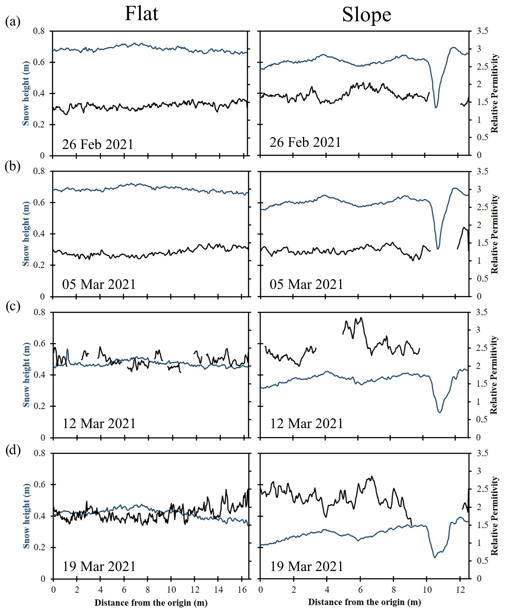
Figure 6 Bulk permittivity (black line) and snow depth (blue line) calculated for the flat (left) and sloped (right) transects on (a) 26 February, (b) 5 March, (c) 12 March and (d) 19 March. Adapted from Valence and Baraer (2021).

4.4 Drone-based GPR permittivity measurement

On each survey day and in each area, snow depth was extracted from the DSM following the north-to-south transects (Fig. 1b) covered by the M600 pro. Snow depth and snowpack bulk permittivity profiles of selected transects are shown in Fig. 6.

On 26 February (Fig. 6a), the flat area showed quite stable bulk permittivity and snow depth profiles, with a relative permittivity ranging from 1.2 to 1.6. The sloped transect exhibited slightly lower snow depth and higher bulk permittivity than the sloped section, between 1.4 and 2. The bulk permittivity over the sloped section appeared more variable than the flat one too. With a relative permittivity ranging from 1.2 to 1.5 and from 1 to 2 for the flat and the sloped areas, respectively, 5 March (Fig. 6b) showed limited changes in bulk permittivity compared to 26 February for both areas.

The 12 March (Fig. 6c) transects showed a sharp change compared to the first two dates. Both areas exhibited a rise in bulk permittivity and a decrease in snow depth. Bulk permittivity profiles showed gaps due to the GPR signal not penetrating fully through the wet snow. They ranged from 1.9 to 2.5 and from 2 to 3.2 for the flat and the sloped areas, respectively. The bulk permittivity in the sloped area had higher values and variability than in the flat area. On 19 March (Fig. 6d), the snow depth in the flat transects remained similar to that measured on 12 March. The bulk permittivity decreased to values situated between those of 5 and 12 March, reaching minimal relative permittivity values of 1.5 in both flat and sloped areas and increasing the value ranges in both flat and sloped areas. The sloped-area transect exhibited a decrease in bulk permittivity, like that of the flat-area transect, and its variability remained higher than in the flat section. The main difference between the two sections was the snow depth. The sloped area showed a more pronounced decrease than the flat area. As no fresh precipitations were recorded between 12 and 19 March, the decrease in permittivity in both sections can be interpreted as a decrease in LWC, which could have occurred together with snow densification in the sloped section.

Overall, Fig. 6 confirms the difference in response to M.E. 2 between the snowpack's sloped and flat areas, including a high moisture content for both areas and a more pronounced densification of the snowpack over the sloped area compared to the flat one.

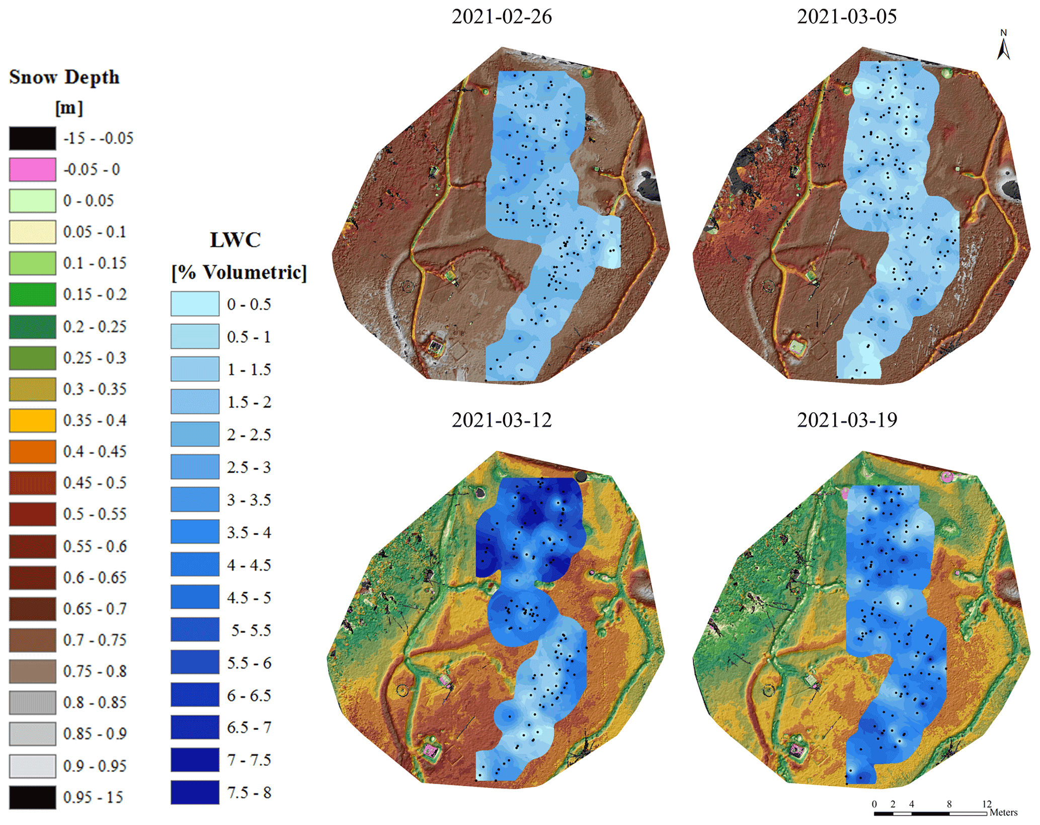
Figure 7 LWC calculated by GPR frequency-dependent attenuation analysis. Points used for interpolation are displayed in black.

4.5 Drone-based GPR frequency-dependent attenuation analysis

Contradicting snow temperature profiles (Fig. 2c) that suggested the snowpack was dry, the LWC calculation and interpolation presented in Fig. 7 suggest non-zero LWC (ranging from 0 % to 3.5 %), with no visible differentiation between the sloped and flat areas on both 26 February (Fig. 7a) and 5 March (Fig. 7b). On both dates, there was a relative spatial heterogeneity in LWC, with no common patterns between the two dates.

On 12 March (Fig. 7c), the flat-area LWC ranged between 0 % and 5.5 %, while the sloped area had LWC maximal values above 8 %. The 12 March survey showed a general increase in LWC compared with the two previous surveys, as well as a differentiation between the two studied areas. The sloped area exhibited the highest overall LWC, although both areas were spatially variable.

Compared to 12 March, 19 March (Fig. 7d) showed overall slightly lower LWC values in the sloped area compared to the flat area. However, the maximum value reached 6.5 % in both areas, making them difficult to differentiate. LWC values remained highly variable for both sections, ranging between 0 and 6.5 %.

Overall, Fig. 7 confirms that, unlike the ROS event that occurred at the end of February, the sloped and flat areas responded in different ways to the 11 March ROS event. On the other hand, LWC values seem unrealistic for the first two survey dates that followed the pronounced cold episode. In a similar way, the absence of a recurrent spatial pattern in LWC variations between maps of different dates suggests the method was not able to capture these variations in a detailed way.

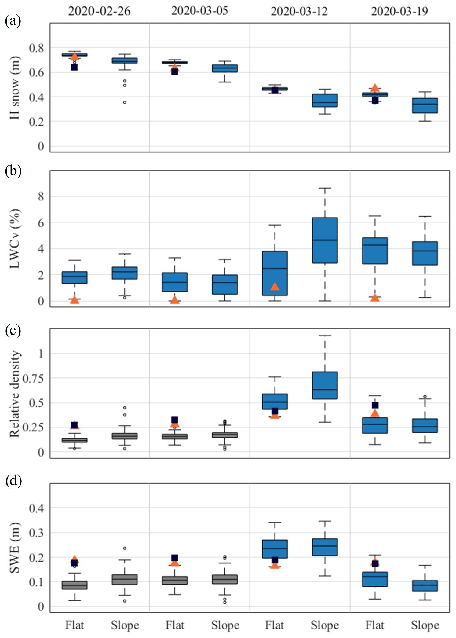
Figure 8 Box plots representing the snowpack studied variables for the sloped and flat areas for each survey date: (a) snow depth results from photogrammetry, (b) liquid water content estimated with drone-based GPR, (c) relative density estimated with drone-based GPR, and (d) snow water equivalent calculated from relative density and snow depth. In the boxes, the central black line represents the median, and the bottom and top edges mark the 25th and 75th percentiles, respectively. The whiskers show the data ranges, excluding outliers. Where they exist, outliers are represented by a black circle. Dark blue squared and orange triangular markers represent reference values originating from the AWS and snow pits, respectively. Grey boxes were calculated with the assumption of a dry snowpack.

5 Discussion

5.1 Drone-based estimation of key snowpack variables

The spatiotemporal variability in snow depth, snow density, SWE and snow LWC, four key properties of a snowpack, has been assessed using drone-based GPR and photogrammetry methods in a repeated way. Figure 8 provides an overview of the variability of those properties in the form of boxplots and, where possible, compares drone-based measurements to those of the AWS and from snow pits.

Photogrammetry snow depth results (Fig. 8a) are in good agreement with those of the AWS and of the snow pits over the entire study period, with a possible slight overestimation in the first two surveys. The differences between the 25th and 75th percentiles in the flat area are systematically below 2 cm. For comparison, this difference is of the same order of magnitude as the one between the snow pit and AWS measurements and the median. The slope is characterized by a lower snow depth and a larger range than the flat area, especially after the ROS event that occurred on 11 March. With most of the slope snow depth values below 40 cm for the last two surveys, the estimated ± 5 cm uncertainty that applies to the photogrammetry affects more than 12 % of the measurement. Such high level of uncertainty may have potential detrimental effects on the GPR-based calculation of key snowpack properties.

The LWC boxplot in Fig. 8b is effective in representing the general evolution of the snowpack moisture content through time: a stable situation occurring between the first two survey dates, followed by a marked increase in snow moisture on 12 March and a slight decrease on 19 March (for the sloped area only). The boxplot also successfully captures the difference in response to mild events between the flat and sloped areas. Compared to the A2 WISe sensor measurements, the boxplot shows the method did not succeed in providing realistic LWC values. According to the A2 measurements, snow pit bulk LWC values were close to 0 % on 26 February and 5 and 12 March, while the GPR-based calculation medians for the flat area were 2 %, 1.5 % and 4 %, respectively. The differences between the 25th and 75th percentiles in the flat area were 1 %, 1.5 % and 2 % for the same dates. Even if the A2 measurements might have been influenced by the sampling constraints and therefore might have underestimated the snowpack average LWC, the drone-based result appears significantly overestimated.

Disagreement between GPR-based calculations and reference measurements was observed for the relative snow density as well (Fig. 8c). On 26 February and 5 March, the difference between reference values and GPR-based calculation medians was 3 times higher than the difference between the 25th and 75th percentiles. The drone-based method underestimated relative snow density over the flat area compared with both the AWS and the snow pit measurements for the first two and the last dates while overestimating it for 12 March. Moreover, both the flat and sloped areas exhibited an unrealistic 50 % decrease in snow relative density between 12 and 18 March. No fresh snowfall occurred between those two dates.

Calculated as the product of h and ρ, SWE boxes show similar biases to relative snow density (Fig. 8d).

Interestingly, we note that while Fig. 6 shows the bulk permittivity profile being consistent with TDR and AWS measurements, this is not the case with the GPR-based computed variables presented in Fig. 8. As described earlier, the bulk permittivity of the snowpack is influenced by both snow density and LWC. Figure 8 therefore suggests that the method we applied failed to differentiate the relative influence of both variables.

The method we applied makes use of empirical Eqs. (7), (8) and (9), which are commonly used in snow hydrology. According to Tiuri et al. (1984), Eqs. (8) and (9) apply to pendular regime, for ${\mathit{\epsilon }}_{\mathrm{s}}^{\prime }\le \mathrm{2.6}$ (${\mathit{\epsilon }}_{\mathrm{s}}^{\prime }\le \mathrm{3}$ for Colbeck, 1982), as opposed to a funicular regime. In a layered snowpack in which preferential flow occurs, it is realistic to hypothesize that both regimes occur in the snow column, making Eqs. (8) and (9) possibly not directly applicable to bulk relative permittivity measurements.

Different empirical formulas relating the relative permittivity to relative snow density have been subsequently developed (e.g., Di Paolo et al., 2018; Frolov and Macheret, 1999). They could possibly represent more accurate alternatives.

As suggested by Webb et al. (2021), reassessing the application conditions of the equation used in the present study is another direction that could be chosen. Selecting different equations depending on snowpack conditions and evolution over the winter could ensure a better use of these equations too.

Fixing the relative density of the snow based on manual sampling or AWS values could represent another solution to the problem encountered in differentiating between the relative influence of snow density and LWC on bulk permittivity. However, this solution would not allow for the capturing of the spatial variability in snow density and therefore might bias calculations.

For spatiotemporal variability in snowpack characteristics, TDR monitoring, drone-based photogrammetry and drone-based GPR have been shown to be a valuable combination for assessing the spatiotemporal variability in key snowpack variables. The use of photogrammetry to map snow depth over the study area provided the opportunity to calculate bulk permittivity from repeated drone-based GPR surveys. Both bulk permittivity and snow depth profiles agreed with site observations and reference measurements. When the bulk permittivity was converted into absolute snow density, LWC and SWE values did not provide the expected results even if the temporal evolution of those parameters was captured in an acceptable way. TDR monitoring complemented the drone-based measurements well, providing both high temporal resolution and layer-based snowpack relative permittivity time series. Snow depth and snow bulk permittivity calculations were highly consistent in comparisons of the different methods to each other, allowing for the capture of the flat- and sloped-area responses to changes in meteorological conditions.

5.2 Points learned from the case study

The application of the proposed methodology to the winter of 2020–2021 led to the following facts being learned.

• The flat and sloped areas had comparable responses to the first ROS event of the study period, which occurred on a cold and dry snowpack at the end of February. That event produced snowpack outflows and increases in LWC, especially at the base of both areas. The sloped area, however, showed a faster and more intense response than the flat one.

• The first ROS episode did not modify the snowpack's snow density and snow depth profiles in a substantial way. Both study areas exhibited characteristics of preferential flow pathways.

• The second ROS event that occurred on 10 March on an already pre-warmed snowpack affected the sloped area in a different way than the flat one, both areas showing important differences in snow depth, LWC and density in the 12 March surveys. The timing and amplitude of the outflow suggest a more homogeneous flow path was present than during the first ROS.

• The third mild episode that occurred from 16 to 18 March did not drastically modify the characteristics of either area compared to the 12 March situation. However, the slope showed faster rates of melt/ablation and showed a higher response to diurnal fluctuations, probably due to its southerly aspect.

6 Conclusion

A combination of TDR monitoring, drone-based photogrammetry and drone-based GPR was used in the experimental watershed of Ste-Marthe (Quebec, Canada) over the winter of 2020–2021. The suite of methods showed comparable snow accumulation over flat and sloped areas, with comparable characteristics lasting after the first ROS event. The second ROS event at the start of the ablation season led to differences in response between the two areas.

Drone-based GPR was very instructive when interpretation was based on bulk permittivity results but showed limitations in mapping snow density, SWE and LWC. There are questions about the applicability of empirical equations used given the site conditions. The results suggest the empirical equations should be reassessed for conditions that differ from the ones for which they were formulated. The method did not allow the researchers to obtain the full benefit from applying the GPR frequency-dependent attenuation method to estimate LWC in the snowpack. The method shows promise, however. In the winter of 2020–2021, the radargram obtained using a 1.5 GHz GPR was not detailed enough to differentiate between the main snowpack layers. However, efforts should be continued in this regard, as the 2020–2021 snowpack was characterized by a relatively low snow depth and an uneven distribution of the ice layers in the snow column.