the Creative Commons Attribution 4.0 License.
the Creative Commons Attribution 4.0 License.
 | 22 Sep 2022
Probabilistic spatiotemporal seasonal sea ice presence forecasting using sequence-to-sequence learning and ERA5 data in the Hudson Bay region
Nazanin Asadi
Philippe Lamontagne
Matthew King
Martin Richard
K. Andrea Scott
Accurate and timely forecasts of sea ice conditions are crucial for safe shipping operations in the Canadian Arctic and other ice-infested waters. Given the recent declining trend of Arctic sea ice extent in past decades, seasonal forecasts are often desired. In this study machine learning (ML) approaches are deployed to provide accurate seasonal forecasts based on ERA5 data as input. This study, unlike previous ML approaches in the sea ice forecasting domain, provides daily spatial maps of sea ice presence probability in the study domain for lead times up to 90 d using a novel spatiotemporal forecasting method based on sequence-to-sequence learning. The predictions are further used to predict freeze-up/breakup dates and show their capability to capture these events within a 7 d period at specific locations of interest to shipping operators and communities. The model is demonstrated in hindcasting mode to allow for evaluation of forecasted predication. However, the design allows for the approach to be used as a forecasting tool. The proposed method is capable of predicting sea ice presence probabilities with skill during the breakup season in comparison to both Climate Normal and sea ice concentration forecasts from a leading subseasonal-to-seasonal forecasting system.
- Article
(11519 KB) - Full-text XML
- BibTeX
- EndNote


Spatial and temporal forecasts of sea ice concentration (fraction of a given area covered by sea ice) are carried out at various scales to address the requirements of different stakeholders (Guemas et al., 2016). Short-term forecasts (1–7 d) at high spatial resolution (5–10 km) are important for day-to-day operations and weather forecasting (Carrieres et al., 2017; Dupont et al., 2015), whereas longer-term (60–90 d) forecasts are desired by shipping companies and offshore operators in the Arctic for strategic planning (Melia et al., 2016). In this study we are interested in these longer-term forecasting methods, which we will refer to as seasonal forecasting. Typical approaches are usually statistical or dynamical in nature. Statistical approaches include multiple linear regression (Drobot et al., 2006) or Bayesian linear regression (Horvath et al., 2020), whereas by dynamical approaches we are referring to those that use a forecast model solving the prognostic equations governing evolution of the ice cover (Askenov et al., 2017; Sigmond et al., 2016). An excellent overview of both statistical and dynamical approaches is given in Guemas et al. (2016).
An early study on seasonal sea ice forecasting using a dynamical approach is that by Zhang et al. (2008), in which they evaluated the ability of an ensemble of sea ice states from a coupled ice–ocean model to predict the spring and summer Arctic sea ice extent and thickness for the year of 2008, following the anomalously warm year of 2007. Each ensemble member was generated by forcing the coupled ice–ocean model with atmospheric states from 1 of the previous 7 years and running the model forward in time for 1 year. Similar to Zhang et al. (2008), the majority of studies on sea ice prediction and forecasting focus on the pan-Arctic domain. A comparison between pan-Arctic and regional forecast skill was carried out by Bushuk et al. (2017), where skill was assessed using the detrended anomaly correlation coefficient (ACC) of sea ice extent. It was shown that the ACC of seasonal forecasts in specific regions was dependent on the region and forecast month.
Dynamical forecast models solve differential equations describing the physics of the underlying system. Solution methods for these types of equations are well-known and relatively robust. A key challenge with these models in operational forecasting is the high level of computational resources required to generate a forecast. This disadvantage can be overcome by using statistical approaches such as multiple linear regression (Drobot et al., 2006) or canonical correlation analysis (Tivy et al., 2011). Both of these approaches determine a linear relationship between a set of predictor variables and a set of predictands.
More recently, convolutional neural networks (CNNs), which are able to learn nonlinear relationships between spatial patterns in input data and predictands, have been used for sea ice concentration prediction (Kim et al., 2020). The study by Kim et al. (2020) used eight predictors composed of sea ice concentration data and variables from reanalyses to train 12 individual monthly models and produced monthly spatial maps of sea ice concentration (SIC). Their method was able to predict mean September sea ice extent in good agreement with that from passive-microwave data, evaluated for the year of 2017, where the sea ice extent is the total area in a given region that has at least 15 % of ice cover. Similar to Kim et al. (2020), Horvath et al. (2020) focused on the September sea ice extent. Horvath et al. (2020) used a Bayesian logistic model to predict both a monthly average sea ice concentration and an uncertainty. The model inputs were atmospheric and oceanic predictor variables and sea ice concentration from satellite data. It was found that the uncertainty was higher at the ice edge, although further analysis of this output was not given. Another recent study by Fritzner et al. (2020) compared two machine learning (ML) approaches, k-nearest neighbor (KNN) and fully convolutional neural networks, with ensemble data assimilation.
A recent approach close to the one presented here is IceNet (Andersson et al., 2021), which trained an ensemble of CNNs to produce monthly maps of sea ice presence (probability SIC>15 %) for forecast lengths up to 6 months. Similar to other studies, input to this model consisted mainly of reanalysis data. A novel aspect was the training protocol, which consisted of pre-training each ensemble member using a long time series of data from the Coupled Model Intercomparison Project phase 6 (CMIP6) and then fine-tuning the trained CNNs using sea ice concentration observations, followed by a scaling method, known in the ML community as “temperature scaling”, to produce a calibrated probability of sea ice presence.
None of the previously proposed ML approaches produce a forecast that propagates in space and time, i.e., a spatiotemporal forecast. In this study we investigate a sequence-to-sequence (Seq2Seq) learning approach to provide daily spatiotemporal forecasts of the probability of sea ice presence (probability SIC>15 %) over the region of Hudson Bay, with forecast lead times up to 90 d. To keep the method general, we use ERA5 data as input to our model. By using the Seq2Seq approach we are able to produce forecasts over a different number of days than our training sequence. The method is similar to operational forecasting studies (Chevallier et al., 2013; Sigmond et al., 2013), where an initial state is propagated forward in time, except we are using a data-driven machine learning approach, as compared to a physics-based model, and our forecasted variable is a number between 0 and 1 that indicates the (uncalibrated) probability of sea ice presence at a grid location, as compared to sea ice concentration.
2.1 ERA5
The present study utilizes ERA5 reanalysis data for model predictors and validation (Hersbach et al., 2018). ERA5 is a recent reanalysis produced by the European Centre for Medium-Range Weather Forecasting (ECMWF). It consists of an atmospheric reanalysis of the global climate providing estimates of a large number of atmospheric, land, and oceanic climate variables. The spatial resolution is ≈31 km, and reanalysis fields are available every hour from 1979–present (Wang et al., 2019). Observations are assimilated into the atmospheric model using a 4D variational data assimilation scheme. In this study ERA5 reanalysis data from 1985–2017 are used.
The sea ice concentration data used in ERA5 are from the EUMETSAT (European Organisation for the Exploitation of Meteorological Satellites) Ocean and Sea Ice Satellite Applications Facility (OSI SAF) 401 dataset (Tonboe et al., 2016). These data are produced using a combination of passive-microwave sea ice concentration retrieval algorithms to benefit from low sensitivity to atmospheric contamination of the surface signal while maintaining an ability to adapt to changes in surface conditions through the use of variable tie points for ice and water (Tonboe et al., 2016). Although the SIC is gridded to a 10 km grid, the spatial resolution of these data is limited by the instrument field of view of the 19 GHz channel used in the SIC retrieval, which is 45 km×69 km. When the SIC data are ingested into ERA5, the SIC values that are less than 15 % are set to zero. Additionally, SIC is set to zero if sea surface temperature (SST) is above a specified threshold to account for known biases in passive-microwave sea ice concentration during melt.
The current study utilizes daily samples with the following eight input variables from the ERA5 dataset over the period of 1985–2017: sea ice concentration, sea surface temperature, 2 m temperature (t2m), surface sensible heat flux, wind 10 m U component (u10), wind 10 m V component (v10), land mask, and additive degree days (ADDs) derived from the t2m variable. All the input variables except sea ice concentration and land mask are normalized before being input to the network. Recalling that data are available from ERA5 every hour, the fields from 12:00 UTC (midday) were used.
There were some irregularities with the ERA5 land mask file and the sea ice concentration. Some locations indicated as land in the land mask file had a non-zero sea ice concentration value. At these locations the sea ice concentration was set to zero. There were also some locations indicated as non-land in the land mask file that had a zero ice concentration, even when the ice concentration should be non-zero based on the atmospheric conditions, season, and examination of the time series at the given location. At these locations we set the sea ice concentration to the average of the non-land neighboring pixels.
2.2 Operational ice charts
Regional ice charts from the Canadian Ice Service (CIS), referred to herein as CIS charts, were used to complement the use of ERA5 for verification of freeze-up and breakup dates. CIS ice charts are compiled by analysts who manually combine data from various sources, including synthetic-aperture radar (SAR) imagery, sea ice concentration from passive-microwave data, optical data, and ship reports. Regional ice charts are available on a weekly or biweekly basis over the study period and fully cover the study domain. Although daily ice charts are available at a higher temporal frequency than regional charts, they are only available during certain times of the year and over certain regions. Due to this non-standard spatiotemporal coverage, daily ice charts were not used. It is important to note the temporal resolution of the CIS regional ice charts is coarse compared to the needs of this assessment.
2.3 S2S forecasts
The subseasonal-to-seasonal (S2S) system by ECMWF (Vitart and Robertson, 2018) was used to complement the use of ERA5 for verification of binary accuracy spatially and across seasons. The S2S predictions are launched twice a week (Monday and Thursday), with forecasts for lead times up to 46 d. For the comparison presented here, the data from our models are extracted for the same launch dates as those used for the S2S system. The S2S data were extracted at a spatial resolution of and interpolated to our 31 km grid resolution using a nearest-neighbor approach. Results are shown only for 2016 and 2017 because these are the years for which forecasts are available for the S2S system that overlap with our study period.
For the present study we focus on the Hudson Bay system, consisting of Hudson Bay, James Bay, Hudson Strait, and Foxe Basin (Fig. 1). The area is bordered by 39 communities, 29 of which are exclusively accessible by sea or air. These communities rely extensively on sea lift operations during the ice-free season to receive their yearly resupply of fuel and goods too heavy to be flown. Shipping traffic, mostly confined during the ice-free and shoulder seasons, is also generated by mining, fishing, tourism, and research activities (Andrews et al., 2018). The study area is seasonally covered by first-year ice, with open water over most of the domain each summer, with the exception of some small regions in Foxe Basin. The seasonal cycle of ice cover in this region is dominated by local atmospheric and oceanic drivers (Hochheim and Barber, 2014). Freeze-up generally starts in November (earlier in the northern part of the region) and lasts for a couple of months. Breakup usually starts in May or June, and the breakup period is a little longer than freeze-up, at 2–3 months. Recent years show earlier breakup and later freeze-up. The trends and their significance are dependent on the region (Hochheim and Barber, 2014; Andrews et al., 2018).
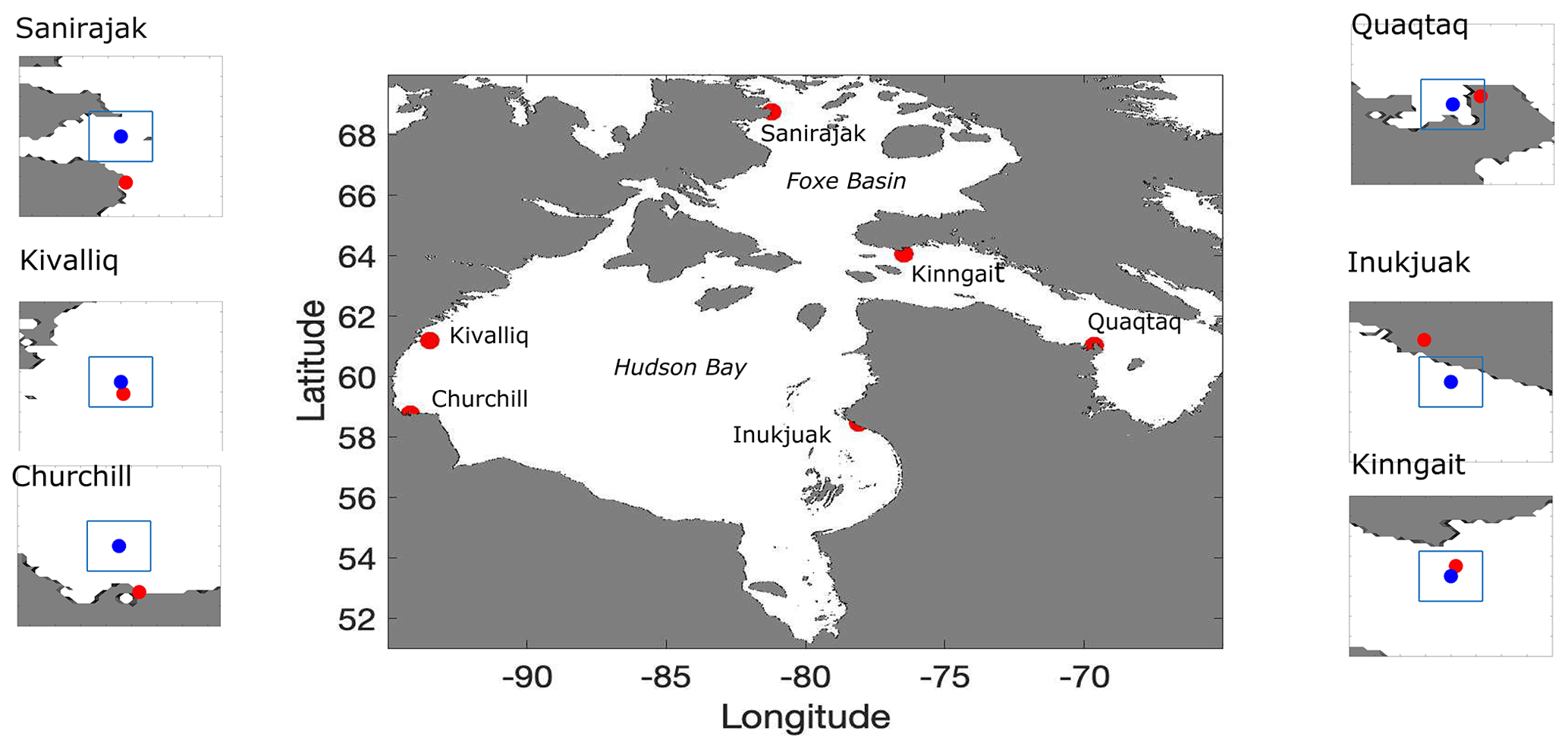
Figure 1The study region with locations of interest shown in red. The insets show the location of a nearby port or polynya (red) and the nearest point on the model grid (blue) that is outside of the land boundary (where the land mask from ERA5 is less than 0.6), in addition to a bounding box that approximates a grid cell. The ports are Churchill, Inukjuak, and Quaqtaq, whereas the polynyas are near Sanirajak, Kivalliq, and Kinngait.
The seasonal forecasting problem of this study can be formulated as a spatiotemporal sequence forecasting problem that can be solved under the general sequence-to-sequence (Seq2Seq) learning framework (Sutskever et al., 2014). In Seq2Seq learning, which has successful applications in machine translation (Cho et al., 2014), video captioning (Venugopalan et al., 2015), and speech recognition (Chiu et al., 2018), the target is to map a sequence of inputs to a sequence of outputs, where the inputs and outputs can be different lengths. The architecture of these models normally consists of two major components: encoder and decoder. The encoder component transforms a given input (here, a set of geophysical variables such as sea ice concentration and air temperature) to an encoded state of fixed shape, while the decoder takes that encoded state and generates an output sequence (here, a sea ice presence probability) with the desired length, which here is the number of days in the forecast (90 d).
For this study, following the encoder–decoder architecture described above, two spatiotemporal sequence-to-sequence prediction models are developed. These will be referred to herein as the “Basic model” and the “Augmented model” and are described in Sect. 4.1 and 4.2 respectively. For both models, the prediction sequence is unrolled over a user-specified number of forecast days to produce ice presence probability forecasts on a spatial grid each day with a scale of ≈31 km (the same as the ERA5 input data).
4.1 Basic model
The encoder section of the Basic model takes the geophysical variables from the last 3 d (sea ice concentration, air temperature, etc.) as input. Each input sample is of size (), where 3 is the number of historical days, W and H are the width and height of the raster samples in their original resolution, and C is the total number of input variables (here 8). Using a longer input sample of 5 d was also tested but did not lead to an improvement in forecast quality. With this longer input the quantity of data to be processed was greater than that for 3 d, which increased the computational expense and data storage requirements; hence 3 d was used for the experiments shown here.
The overall architecture is shown in Fig. 2a. The encoder starts by passing each input sample through a feature pyramid network (Lin et al., 2017) to detect spatial patterns in the input data at both the local and large scales. Next, the sequence of feature grids extracted from the feature pyramid network are further processed through a convolutional LSTM (long short-term memory) layer (ConvLSTM) (Hochreiter and Schmidhuber, 1997; Xingjian et al., 2015), returning the last output state. This layer learns a single representation of the time series that also preserves spatial locality. The most recent day of historic input data is concatenated with the ConvLSTM output to better preserve the influence of this state on the model predictions. The encoder provides as output a single raster with the same height and width as the stack of raster data input to the network but with a higher number of channels such as to fully represent the encoded state. The final encoded state is then fed to a custom recurrent neural network (RNN) decoder that extrapolates the state across the specified number of time steps. It takes as input the encoded state with multiple channels and as output produces a state with the same height and width as the input over the desired number of time steps in the forecast (here 90 d). Finally, a time-distributed network-in-network (Lin et al., 2013) structure is employed to apply a 1D convolution on each time step prediction to keep the spatial grid size the same but reduce the number of channels to one, representing the daily probabilities of sea ice presence over the forecast period (up to 90 d).
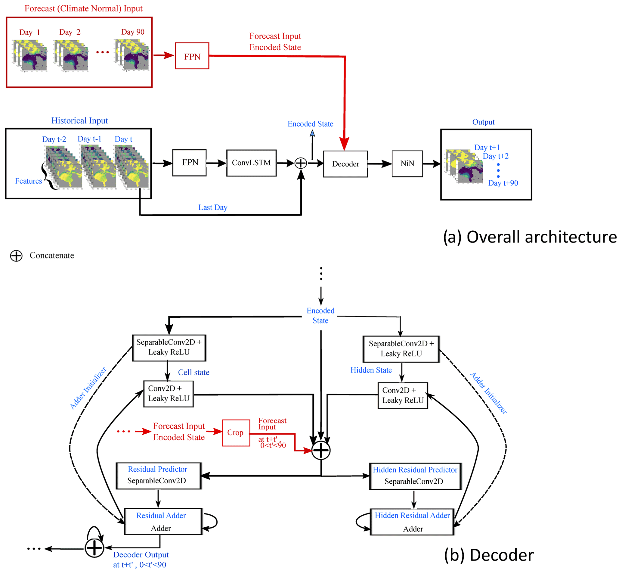
Figure 2(a) Overall network architecture and (b) custom decoder. The black portion in panel (a) refers to the Basic model, while the red portion in panel (a) refers to the additional components required for the Augmented model. The dashed arrows show a process carried out only once (the initialization of the adder). FPN: feature pyramid network, ConvLSTM: convolutional long short-term memory network, NiN: network in network module, ReLU: rectified linear unit.
The custom RNN decoder, shown in Fig. 2b, as is common of many RNN layers, maintains both a cell state and a hidden state (Yu et al., 2019). First, the initial cell state and hidden state are initialized with the input-encoded state. Then, at each time step and for each of the states, the network predicts the difference, or residual, from the previous state to generate the updated states using depthwise separable convolutions (Howard et al., 2017). The output of the decoder section is the concatenation of the cell states from each time step.
4.2 Augmented model
A slight variant of the Basic model, referred to as the Augmented model, is developed to accept a second input. This second input has the same height and width as the first input but corresponds to Climate Normal of three variables over the required period (e.g., 90 d), where these variables are t2m, u10, and v10 and their Climate Normal is calculated from 1985 to the last training year for each forecast day. These variables were chosen because of their availability in both historical datasets and real time (for this application, through the Meteorological Service of Canada GeoMet platform). Since this branch of the network “augments” the core model, it was desired to keep this flexibility for future development, as our computing infrastructure is designed to connect with GeoMet. For the Augmented model, the original encoder structure for historical input data remains unchanged, but a secondary encoder is added to the network, consisting of a feature pyramid network that receives the Climate Normal data as input. A secondary variant of the decoder component is implemented which accepts this encoded sequence in order to enhance estimates of the residuals at each of the future time steps (see Fig. 2).
Since the overarching goal is to provide a tool to stakeholders that can be used operationally, a training and validation protocol is required that truly assesses the forecasting skill without using future data. For example, on this basis a leave-one-out approach cannot be used. Instead, we initially train over a given number of years, and then we update the model weights for future training periods, where the model weights are the learned parameters that transform the input to the output. We tested different initial training periods (10 versus 20 years) and also different numbers of months to include in training our monthly models. The current protocol (Fig. 3) led to the best results.
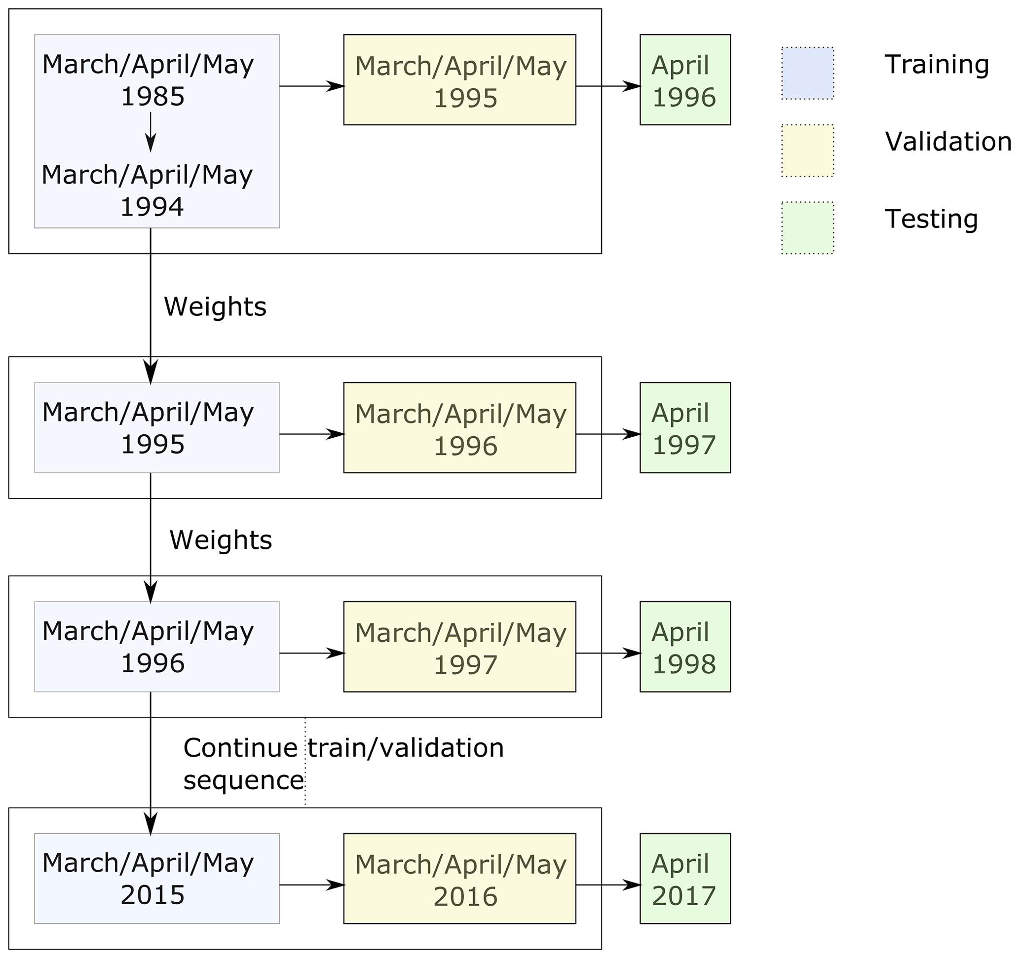
Figure 3Training, validation, and test protocol used for both the Basic and Augmented model.
In this protocol for each month of a year a separate model is trained on data from the given month as well as the preceding and following month. For example, the “April model” is trained using data from 1 March to 31 May. This monthly model is initially trained on data from a fixed number of years, chosen to be 10 years, as a compromise between having enough data to provide the model with representative conditions from which it can learn while allowing for enough data to be set aside for validation and testing. After this initial experiment, to predict each following test year i, using a rolling forecast prediction, the weights of the model from year i−1 are updated with data from year i−2. Data for year i−1 are used as validation for early stopping criteria and to evaluate the training performance. For example the “year 2003” model is initialized with weights from the year 2002 model, which are updated with data from year 2002, validated on year 2003, and used to predict year 2004. This process is used to produce forecasts of sea ice presence for years 1996 to 2017. Since the weight updates use only data of 1 year for training and validation, the method is computationally fast and efficient.
The ML models are implemented using the TensorFlow Keras open-source library with a stochastic gradient descent (SGD) optimizer with a learning rate of 0.01, momentum of 0.9, and binary cross-entropy loss function. The maximum training epoch for the initial model and the retraining process is 60 and 40 respectively, and for both cases the training process stops if the validation accuracy is not improved after 5 epochs.
In order to evaluate the performance of the ML models, the binary accuracy, Brier score, and accuracy of freeze-up and breakup dates are used. The main observations to which model forecasts are compared to are the ERA5 sea ice concentration (thresholded at 15 % to convert to sea ice presence). Based on our training, verification, and testing procedure, the ERA5 states used as observations are from future dates; hence there is a degree of independence from the data used to train the model. To provide a baseline, we also compare our ML models to a Climate Normal, which is defined here as the average of the ERA5 sea ice presence from 1985 to the last year in the training set for each experiment. While inputs of each model in the training and test procedure are derived from 3 months of each year, only the results from the central month (second of three) are selected to evaluate the results of the given model. For example, the April model is trained using historical data from March–April–May. This model is evaluated using 90 d forecasts launched during the month of April. Other datasets used for comparison are sea ice concentration from the ECMWF S2S forecasting system and operational ice charts (described in Sect. 2.2).
6.1 Binary accuracy
Binary accuracy is calculated by mapping the ML model forecasts, which denote a probability of sea ice presence, to binary values by thresholding the probability such that when P>0.5 the pixel is considered to be ice and when P≤0.5 it is considered to be water (similar to Andersson et al., 2021). After this thresholding, the binary accuracy is calculated as , where TP denotes a true positive and has a value of one if both the pixel in the model and observations are one (indicating ice) and a value of zero otherwise, TN denotes a true negative and has a value of one if both the pixel in the model and observations are zero (indicating water), and N is the total number of pixels considered. When binary accuracy is used to calculate monthly scores for the entire domain (Fig. 4), N is the product of the number of pixels in the spatial domain, the days in the given month, and the number of years over which the forecasts are evaluated. For binary accuracy a score of one is considered optimal.
6.2 Brier score
Binary accuracy scores do not differentiate between a predicted probability of 0.51 and 0.9. Both would be a true positive if the pixel is ice in the observations. Small changes in the predicted probability around the probability threshold impact the binary accuracy. An alternative score that better reflects the value of the predicted probability is the Brier score (BS) (Ferro, 2007):
where Pt,i is the model prediction (sea ice presence probability), Ot,i is the corresponding observation (zero or one) at time t and pixel i, M represents the total number of pixels in the spatial domain, and T is the total number of temporal outputs used (note ). For the Brier score a value of zero is considered optimal.
6.3 Freeze-up and breakup accuracy
The accuracy of the model in predicting freeze-up and breakup dates is indicative of operational capability of the trained models to support shipping operations during the shoulder season. Following the definition used by the Canadian Ice Service (CIS), the freeze-up date of each pixel in a year is the first date in the freeze-up season (1 October to 31 January for Hudson Bay) that ice (value of one after thresholding the predicted probabilities at 50 %) is observed for 15 continuous days. A similar procedure is carried out to predict breakup, with the exception that the pixel must be considered water (value of zero after thresholding its predicted probability) for 15 continuous days for breakup to have occurred in the breakup season (1 May to 31 July for Hudson Bay, with forecasts initialized up to 31 July considered). These freeze-up/breakup dates per pixel per year are calculated for observations, Climate Normal, and model predictions at 30 and 60 lead days. To obtain each accuracy map, first the predicted and observed freeze-up/breakup dates per pixel per year are compared. If the two dates are within 7 d of each other, the prediction is correct (a value of one is assigned), and if not, the prediction is incorrect (a value of zero is assigned). Then, the results are averaged over the total number of years to obtain an overall score between 0 and 1, which we will refer to as freeze-up/breakup accuracy.
7.1 Forecasts of ice presence
7.1.1 Monthly averaged results
For each day in the test set, which is the set of days over which the 90 d predictions are launched, we have 90 binary accuracy maps of our study region. The monthly statistics are summarized in Fig. 4a–c. The value at index (i,j) of each panel of Fig. 4a–c represents the average binary accuracy score of all predictions in the test set that are launched at month i at lead day j, where and . The (1,1) index value of Fig. 4a shows the binary accuracy of 1 d forecasts launched between 1 and 31 January, ending 2 January to 1 February. The (1,2) index value corresponds to the binary accuracy of 2 d forecasts. These forecasts were launched between 1 and 31 January, ending 3 January to 2 February. The (2,1) index value corresponds to the binary accuracy of 1 d forecasts launched between 1 and 28 February, ending 2 February to 1 March.
Binary accuracies (Fig. 4a–c) are close to 100 % for the month of January and for lead times that cover the months of January, February, and March, as would be expected, because at this time the region is covered with ice. In contrast, for forecasts at the beginning of the open-water season (June and July), Climate Normal struggles to accurately capture the ice cover for lead times of 1 to 50 d (Fig. 4a), likely due to interannual variability and lengthening of the open-water period (Hochheim and Barber, 2014; Andrews et al., 2018). The Basic and Augmented models have higher accuracies than Climate Normal over these months (Fig. 4d and e). We also note improvements in the Basic and Augmented models at short lead times for August, September, October, and November, as compared to Climate Normal (Fig. 4d and e). Improvements with the Augmented model can be seen in particular for longer lead times in July/August and at shorter lead times (15–50 d) for November (Fig. 4f). These forecasts correspond to the freeze-up period, which starts in mid-October or November in the study region and lasts for approximately 2 months (Hochheim and Barber, 2014).
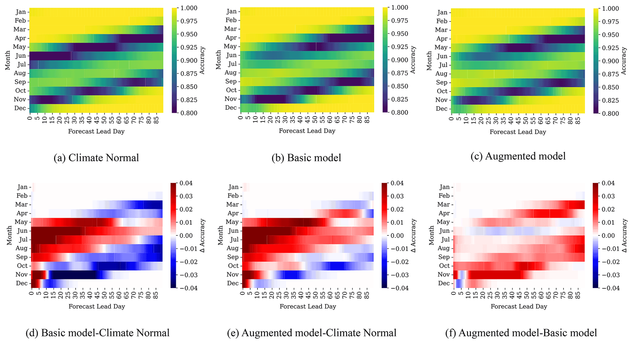
Figure 4Binary accuracies as a function of lead time. Top row panels a–c show the binary accuracy of each model, while bottom row panels d–f show the differences in binary accuracy between the models. The Augmented model is trained with additional 90 d Climate Normal input. Most differences are observed in the breakup and freeze-up seasons.
Figure 5 presents the monthly averaged Brier scores for the Basic and Augmented models (Fig. 5a and b) and their differences (Fig. 5c) as a function of lead days. Similar to Fig. 4, each value at index (i,j) of Fig. 5a–b represents the average Brier score of all predictions in the test set that are launched at month i at lead day j, where and . The resulting pattern is similar to that for binary accuracy. Recalling that a Brier score of zero is optimal, the higher Brier scores seen during freeze-up and breakup for both models indicate poorer performance during these seasons. Their difference (Fig. 5c) indicates a better score for the Augmented model at longer lead times especially for March, April, July, and August. In contrast for some cases like forecasts of 60–90 lead days of the September model, the Brier score of the Basic model is around 0.01 better than the Augmented model. The reason for the higher Brier score of the Basic model in comparison to the Augmented model may be because the September model uses training data over August–October. The trend over this period may be less representative of more recent ice conditions (Hochheim and Barber, 2014; Andrews et al., 2018), which may make the additional data used in the Augmented model unhelpful at these longer forecast periods.
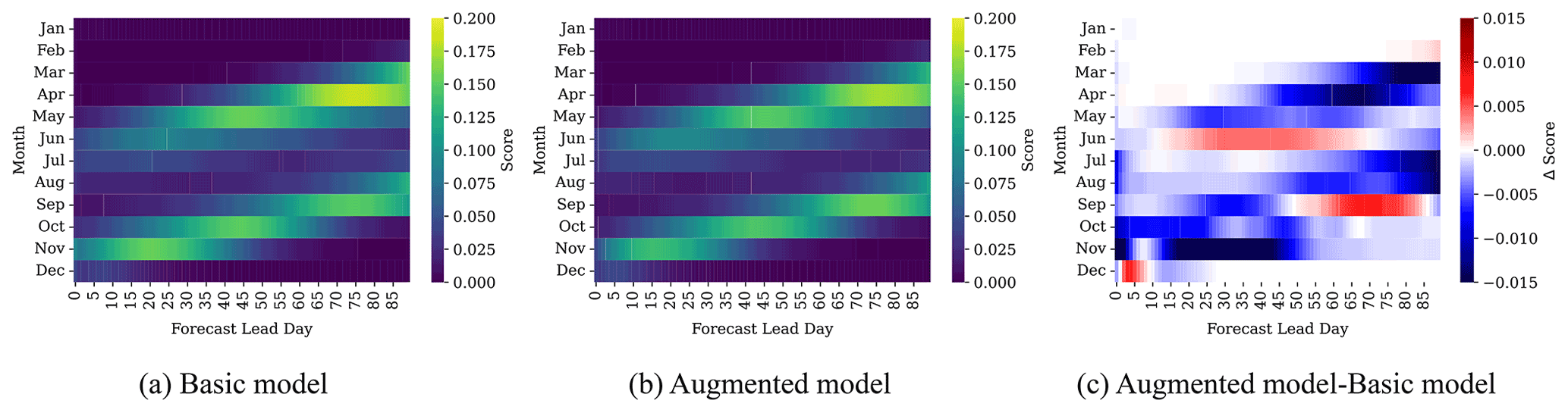
Figure 5Brier score of the (a) Basic and (b) Augmented model as a function of lead time. Their score difference is shown in (c). Most differences are observed in the breakup and freeze-up seasons.
The calibration curves of the Basic and Augmented September models are shown in Fig. 6. These curves represent the observed frequency of ice presence, where the frequency is calculated over the entire domain, versus the forecasted probabilities for different lead days of forecasts launched in September. For short lead times both models, especially the Basic model, show close to perfect calibration (blue line), but at 60 lead days the underestimation is more significant for the Augmented model with lower forecasted probabilities of ice in comparison to observations, while at 90 lead days the overestimation is more significant for the Augmented model, with a forecasted probability that is much higher than the observed frequency of ice. This suggests that in comparison to observations, freeze-up may be delayed at 60 lead days for regions with freeze-up dates around November and may be too early at 90 lead days for regions with freeze-up dates around December for the Augmented model.

Figure 6Calibration curves for the Basic and Augmented model for sea ice presence forecasts initiated from 1 to 30 September for different lead days. At 90 lead days, both models underestimate the probability of sea ice when observed frequencies are less than 0.75 and overestimate the probability of sea ice at higher probabilities. The Basic model is well-calibrated for short lead times.
7.1.2 Spatial maps of sea ice presence
Binary accuracy values averaged over the domain and each month do not provide information about model performance at each location in the spatial domain or at a finer timescale. The model proposed here provides a spatial map of the probability of ice for each day in the forecast period. In Fig. 7 the spatial distribution of ice and water is shown with the probability of ice for three different dates during the breakup period. The observations are ice and water obtained by applying a threshold of 15 % to SIC from ERA5 for the given date. For example, given that the forecasts are launched on 6 May 2014, the left column (after 30 d) corresponds to the sea ice state on 5 June 2014.

Figure 7Spatial patterns of sea ice presence during breakup. These models are trained using data from May, June, and July. The forecasts are launched on 6 May 2014 and are displayed after 30 d (5 June, left column), 50 d (25 June, middle column), and 70 d (15 July, right column).
The forecast after 30 d indicates both the Basic and Augmented models predict a reduced ice presence probability along the eastern coast of Hudson Bay that is in better agreement with observations than Climate Normal. Similarly, after 50 and 70 d, Climate Normal has a higher ice cover relative to the lower probability of ice for the Basic model in the central part of Hudson Bay, while the Augmented model is in better agreement with observations. In comparing the probability maps for the Basic and Augmented model, it can be noted the Basic model has reduced ice presence probability in the southern part of the domain. Overall we find the spatial pattern of breakup to be in good agreement with the observations, in particular for the Augmented model.
7.2 Assessment of operational freeze-up and breakup date forecasting
7.2.1 Freeze-up and breakup in comparison with ERA5 data
We start our comparison using ERA5 as the baseline, consistent with our earlier comparisons. Figures 8 and 9 show the freeze-up and breakup accuracy maps of the Climate Normal as well as the Basic and Augmented model for 30 and 60 lead days. The freeze-up accuracy maps (Fig. 8) show similar spatial patterns for the Basic and Augmented models for 60 lead days, with differences between the two models for 30 lead days. The freeze-up accuracy for 30 lead days looks very different also from Climate Normal. To investigate the prediction of freeze-up by the Basic model at 30 lead days, we looked at forecasts from the November and October models for 30 and 60 lead days respectively, as freeze-up mainly happens in December. It was found (not shown) that the December sea ice presence accuracy of the Basic model at 30 lead days is lower in the central region and higher in Hudson Strait compared to other methods, which explains the difference in freeze-up prediction maps. The poorer accuracy in the central region is because freeze-up was too late, as discussed further in Sect. 8.
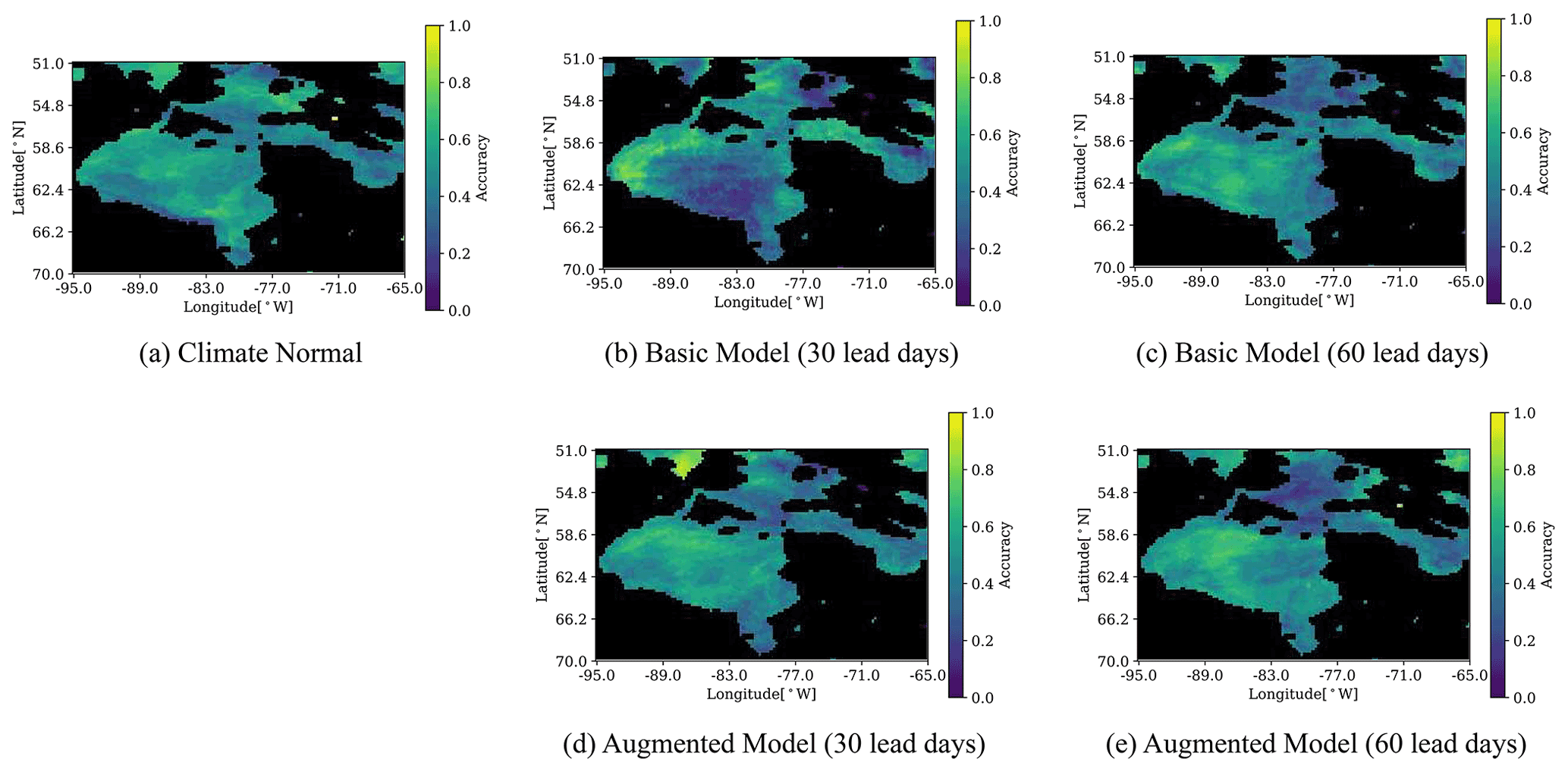
Figure 8Accuracy of the predicted freeze-up date within 7 d. Freeze-up dates are checked from 1 October to 31 January. The 7 d window is chosen to match to the definition used by the Canadian Ice Service.
In contrast to freeze-up, for the breakup accuracy the Climate Normal (Fig. 9a) has an overall poor accuracy, while the Augmented model at 30 lead days (Fig. 9d) has the best accuracy, especially in the central region. The breakup prediction accuracy degrades at 60 lead days for both the Basic and Augmented models.
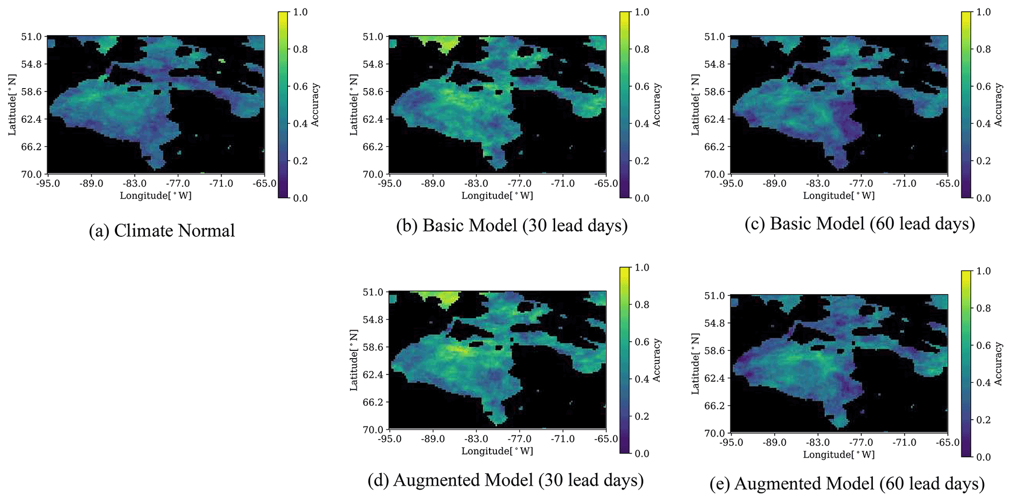
Figure 9Accuracy of the predicted breakup date within 7 d. Breakup dates are checked from 1 May to 31 July. The 7 d window is chosen to match to the definition used by the Canadian Ice Service.
The interannual variability in accuracy in freeze-up (1 October to 31 January) and breakup (1 May to 31 July) predictions is presented in Fig. 10 for 30 and 60 lead days. The respective trends are shown by dashed lines. While no significant trend is observed for freeze-up accuracy at both lead times, the breakup accuracy (Fig. 10c and d) shows a declining trend of 2 %. Similar to Fig. 9 for freeze-up/breakup date predictions, both the Augmented and Basic models have their highest improvement compared to Climate Normal for breakup at 30 lead days. In addition, for both cases, 2010 shows an extreme case where Climate Normal has the lowest accuracy over the entire period. For that year, the Augmented model has a lower freeze-up accuracy compared to other years, while its breakup accuracy does not show any significant variability over the years. It has been noted in an earlier study that 2010 was an anomalous year (Hochheim and Barber, 2014).
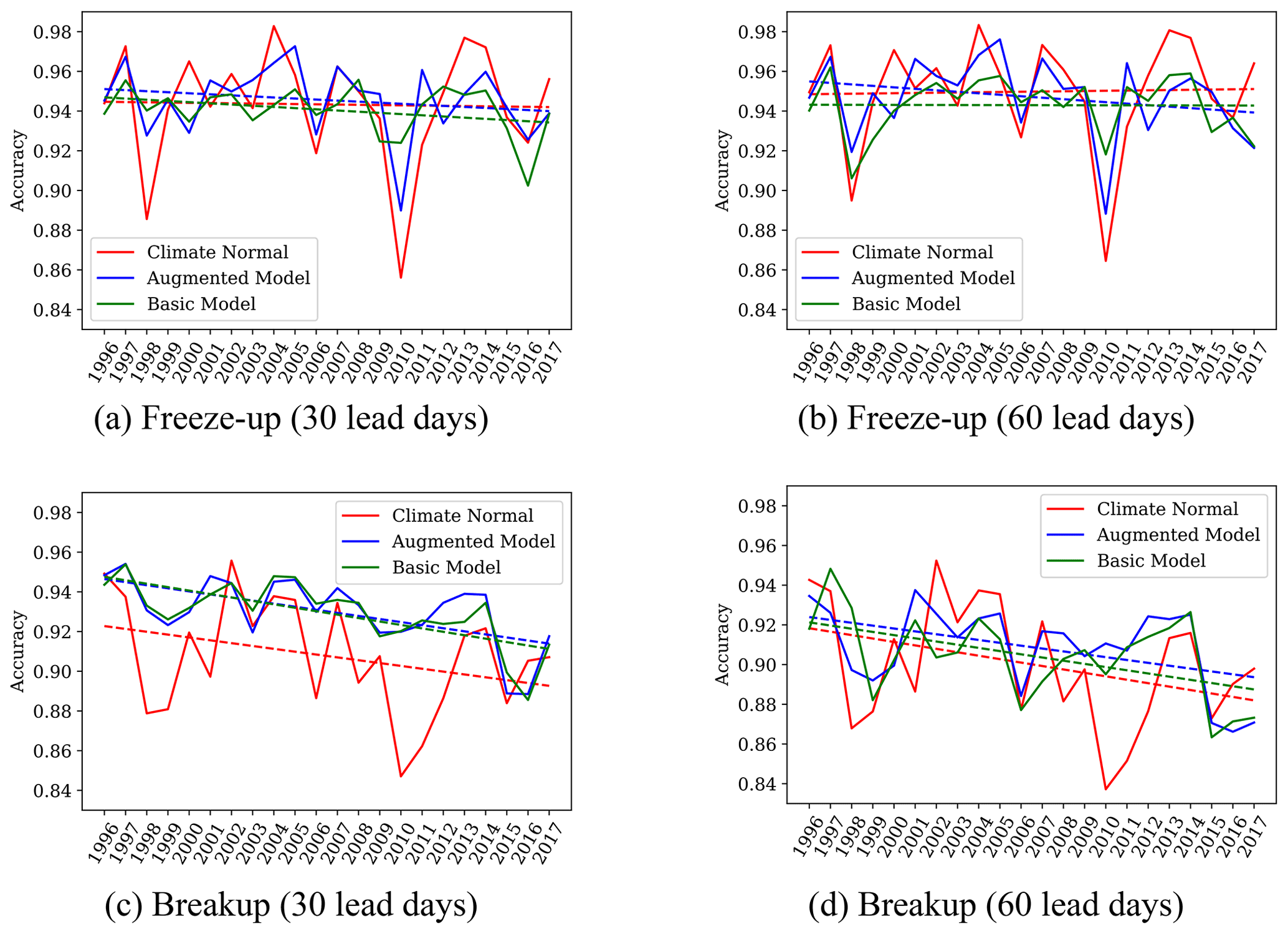
Figure 10Accuracy of the Climate Normal, Basic model, and Augmented model freeze-up and breakup predictions over the years at 30 and 60 lead days. Dashed lines show the trend.
The ability of the model to predict freeze-up and breakup dates can provide helpful information for local communities and shipping operators. Here, the nearest pixels to three sample ports shown in Fig. 1, Churchill, Inukjuak, and Quaqtaq, and Sanirajak (formerly known as Hall Beach) are selected. The sites were chosen because they represent locations with significantly different sea ice conditions. Churchill and Inukjuak are located on the eastern and western coasts of Hudson Bay, with Churchill being a major port as part of the potential Arctic Bridge shipping route. The eastern coast is significantly impacted by freshwater inflow from rivers draining into Hudson Bay, while the region of the western coast is impacted by northwesterly winds (there is a latent heat polynya, the Kivalliq polynya, that runs along the northwest shore of Hudson Bay; Bruneau et al., 2021). There are additionally east–west asymmetries in Hudson Bay in terms of ice thickness and sea surface temperature (Saucier et al., 2004), with counterclockwise ocean currents leading to thicker ice cover along the eastern shore of the bay. Quaqtaq is located in Hudson Strait, where wind and air temperature patterns are different from those in Hudson Bay and pressured ice is common.
Freeze-up/breakup date predictions of the models at 30 and 60 lead days versus observed dates are presented in Figs. 11 and 12. The red line in each plot represents a perfect one-to-one prediction, and the pink region shows the acceptable 7 d difference that will still be considered a correct prediction according to the CIS criteria. The width of the pink zone on each plot varies, as the total timeframe of breakup and freeze-up at each location is different (i.e., the subplots have different x and y axes). In addition, the year of 2010 is omitted from these plots, as it was an anomalously warm year (Hochheim and Barber, 2014).

Figure 11Comparison between forecast and observed freeze-up dates at pixels located in the vicinity of ports in the study region for 30 and 60 lead days. Each dot represents 1 year. The red line represents perfect predictions, and the pink area represents ±7 d of the red line, which is commonly assumed to be an acceptable error range.

Figure 12Comparison between forecast and observed breakup dates at pixels located in the vicinity of ports in the study region for 30 and 60 lead days. Each dot represents 1 year. The red line represents perfect predictions, and the pink area represents ±7 d of the red line, which is commonly assumed to be an acceptable error range.
For freeze-up, 30 lead days predictions are more concentrated and closer to the pink zone, while there is more dispersion and outliers observed for predictions for 60 lead days (Fig. 11). In addition, predictions of the Augmented model have fewer outliers than predictions of the Basic model. For the port of Churchill, predictions are close to the center and inside or close to the pink zone for both models and both lead times compared to other locations. The Basic model, especially at 30 lead days, predicts freeze-up dates of several years with a consistent delay for Inukjuak, while for Quaqtaq its predictions are earlier than observed dates. In Fig. 12, similar to freeze-up, breakup dates are better captured by the Augmented model at 30 lead days as compared to 60 lead days, where predictions are more scattered. Also, the patterns of early and delayed predictions are not as visible for breakup as for freeze-up for the Inukjuak and Quaqtaq ports.
7.2.2 Freeze-up and breakup in comparison with operational ice charts
To assess the operational capability of the models, it is important to consider the authoritative source of information used by shipping operators as a baseline for comparison, which is operational ice charts. Three sites were selected for this assessment: the Kivalliq polynya near the Arviat port (61.19∘ N, 93.49∘ W), Kinngait (64.05∘ N, 76.48∘ W), and Sanirajak (68.83∘ N, 81.10∘ W). These sites were selected because each is both near a port location and associated with a polynya; therefore the ice cover is challenging to predict. The accuracy of freeze-up and breakup dates at each site was evaluated against both CIS regional ice charts and ERA5 baselines. The predictions of the Basic and Augmented models at 30 and 60 lead days were assessed using the mean absolute error (MAE) and accuracy within 7 d. Median breakup and freeze-up dates derived from CIS regional ice charts from 1980 to 2010 and published in the Canadian Ice Service's Ice Atlas 1980–2010 (CIS, 2013) are also evaluated using the same methodology. For the Sanirajak site, each time breakup was outside the date range defined by the extraction methodology (1 May to 31 July) from the ERA5 baseline or model forecast; the missing date was replaced by the ice atlas freeze-up date, 22 October, in order to calculate both metrics. This was done in order to handle a multiyear ice situation when no breakup dates are available.
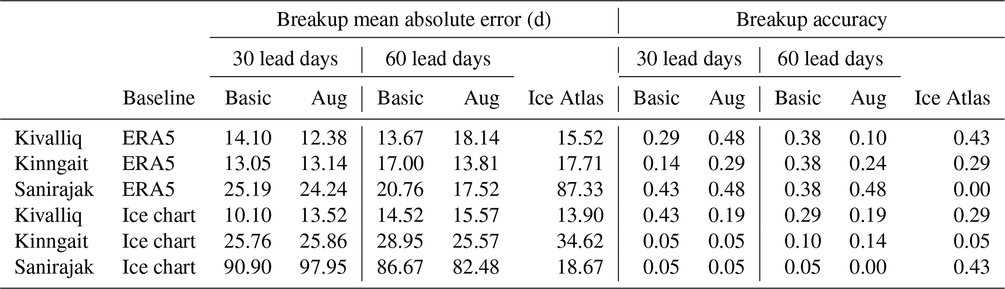
For breakup, at the Kivalliq site, the Augmented model at 30 lead days showed the best performance based on MAE and accuracy metrics using ERA5 as the baseline, while the Basic model at 30 lead days tends to perform better using CIS ice charts as the baseline (Table 1). The breakup dates for the Kinngait site have higher interannual variability, reflected by the poor performance of the ice atlas at this site for both baselines. At the Kinngait site the breakup forecast skill is relatively consistent for both Basic and Augmented models at 30 and 60 lead days but shows higher skill using the ERA5 baseline compared to the ice charts. The difference in breakup dates derived from the two baselines is significant at this site (Table 3), where events such as early breakup in March 2012 are captured by the ice charts but not by the ERA5 reanalysis. For the Sanirajak site, the difference between baselines is exacerbated. The ice charts consistently detect early breakup at this site, while the ERA5 reanalysis does not. For example, the majority of breakup dates derived from ice charts were before 1 July, whereas this occurs only once in 2016 using the ERA5 baseline. The baseline discrepancy explains why the Basic and Augmented models performed better using the ERA5 baseline, while the ice atlas has better skill using the CIS ice chart baseline. However, both have similar skill using their corresponding baseline.
Table 1Breakup mean absolute error and accuracy at selected sites using data from the CIS Ice Atlas, Basic, and Augmented (Aug) models at 30 and 60 lead days versus baseline observations derived from CIS regional ice charts and ERA5.
For freeze-up, at the Kivalliq site, all models perform well, with the lowest freeze-up accuracy at 0.52 using the ERA5 baseline or 0.43 using the CIS ice chart baseline (Table 2). For all sites, the ice atlas showed the highest freeze-up forecasting skill against both baselines, due to the lower interannual variability in freeze-up dates compared to breakup dates. These results are consistent with the freeze-up and breakup accuracy maps (Figs. 8 and 9).
Table 2Freeze-up mean absolute error and accuracy at selected sites using data from the CIS Ice Atlas, Basic, and Augmented (Aug) models at 30 and 60 lead days versus baseline observations derived from CIS regional ice charts and ERA5.
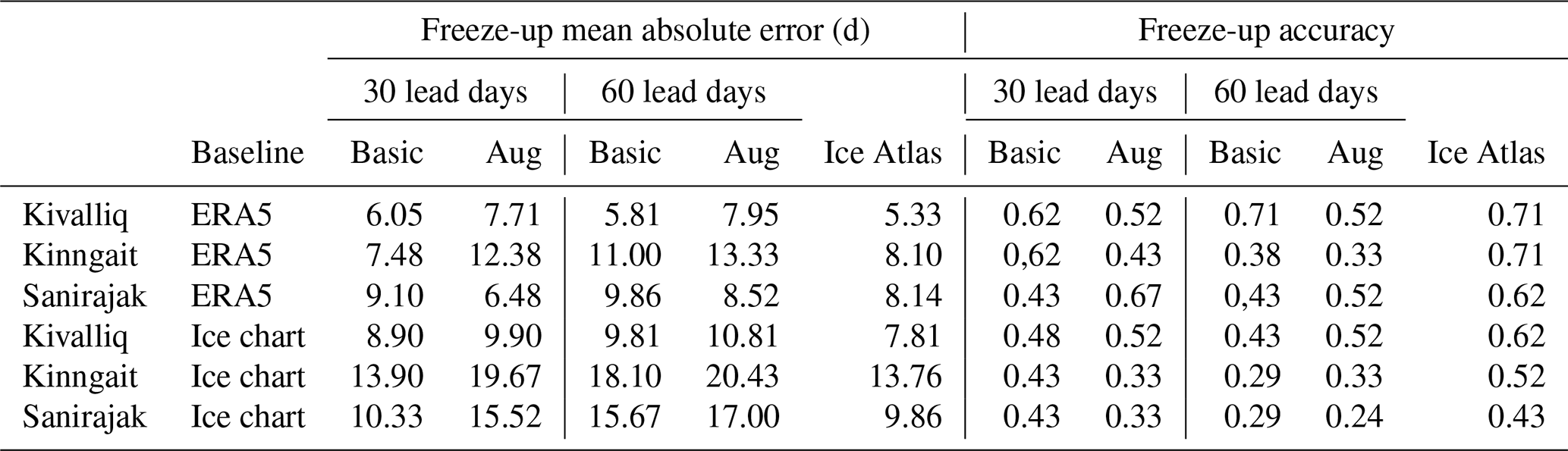
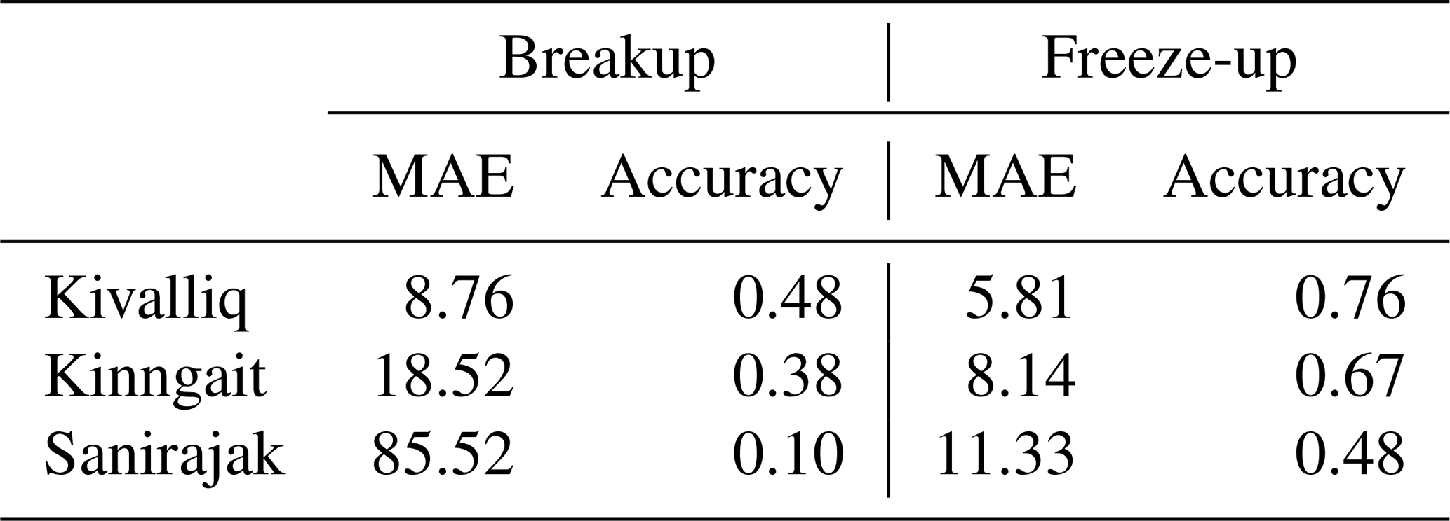
Table 3 highlights the discrepancy between the two baselines using the same metrics as Tables 1 and 2, where MAE can be interpreted as the mean absolute difference between the two baselines and the accuracy can be interpreted as the fraction of the time the baseline dates are within 7 d of each other. As expected, there is a minimal discrepancy for large and uniform areas such as the Kivalliq site, explained by the weekly publication frequency of the CIS regional ice charts. The discrepancy is higher for smaller and localized polynyas, such as the Kinngait and Sanirajak sites, where the low-resolution passive-microwave instruments used by ERA5 do not detect them compared to CIS regional ice charts, which rely in part on higher-resolution SAR data.
Table 3Discrepancy between breakup and freeze-up dates derived from ERA5 and CIS regional ice charts. MAE refers to the mean absolute error (days). Accuracy is the fraction of freeze-up or breakup events for which the baseline dates are within 7 d of each other.
7.3 Comparison with forecast data from the ECMWF S2S system
To evaluate our approach further, binary accuracies are calculated using sea ice concentration from the ECMWF S2S system as the baseline for comparison. Results are shown only for forecasts launched during months for which there are notable differences between the methods, which are May–June and October–November. Figure 13 shows that during May and June both the Basic and Augmented models have a higher binary accuracy than the S2S forecasts, while during October and November the opposite behavior is observed, with the Basic and Augmented models having similarly low accuracies. We investigate these differences using false-positive and false-negative rates. The false-positive rate is and is the ratio of the number of days for which water is incorrectly classified as ice (false positives, ℱ𝒫) to the total number of days classified as water (ℱ𝒫+𝒯𝒩), where 𝒯𝒩 is the true negatives, or number of days correctly classified as water. The false-negative rate is and is the ratio of the number of days for which ice is incorrectly classified as water (false negative, ℱ𝒩) to the total number of days classified as ice (ℱ𝒩+𝒯𝒫), where 𝒯𝒫 is the true positives, i.e. number of days correctly classified as ice. Recall the observation used is the thresholded sea ice concentration from ERA5.
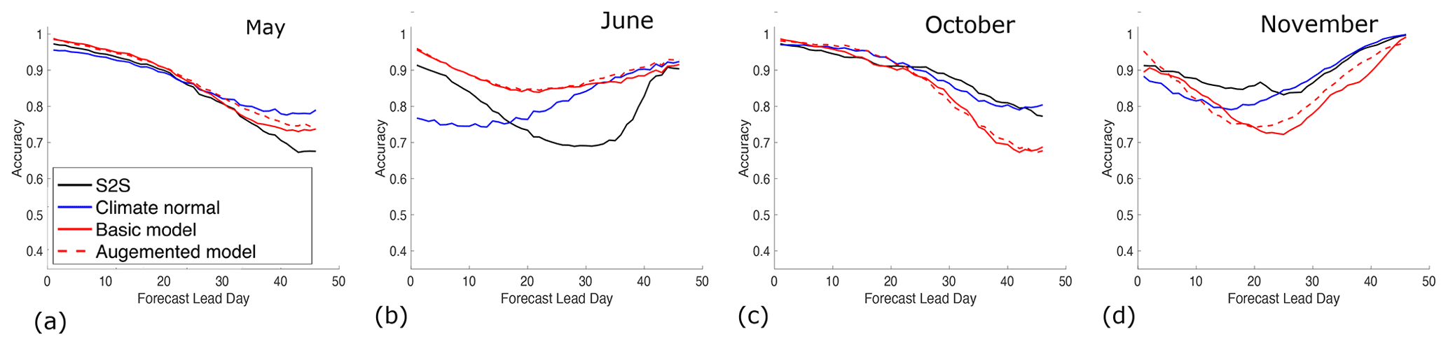
Figure 13Binary accuracy as a function of lead day for forecasts launched in (a) May, (b) June, (c) October, and (d) November. These months were chosen because they display the largest differences between the various forecasting methods. Binary accuracies are evaluated using data from both 2016 and 2017.
Figure 14 shows spatial maps of the binary accuracy, false-positive rates, and false-negative rates, for forecasts at 30 lead days launched on dates between 1 June and 30 June. These forecasts correspond to ice conditions from 1 July to 30 July. The white regions correspond to locations masked out due to land or where there are no positives (days classified as ice) in the false-positive plots and similarly in the false-negative plots. For example, there is no ice in the northwest portion of the domain at this time of the year. For the Basic and Augmented models there is a high false-positive rate in the southeastern portion of Hudson Bay, indicating the sea ice is not retreating fast enough relative to the observations. However, for the S2S forecasts the false-positive rate is high over almost all of Hudson Bay, including Hudson Strait. Climate Normal has the lowest false-positive rate of the approaches examined here. For the false-negative rate, different behavior is observed with a high false-negative rate for Climate Normal, indicating too much open water, and slightly lower false-negative rates for the Basic and Augmented models. The Augmented model has a higher false-negative rate than the Basic model, suggesting some of the overprediction of open water may be related to the additional air temperature or wind speed data that are input to this model. The strong recovery of the binary accuracy of the S2S forecasts around day 35 (Fig. 13b) is due to the ice quickly retreating in these forecasts (not shown).
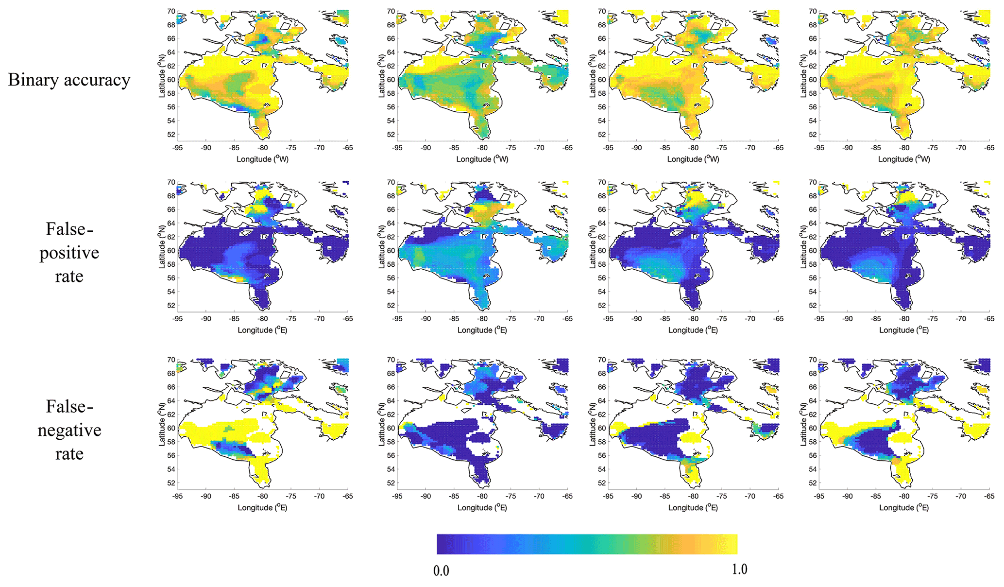
Figure 14The columns from left to right are as follows: Climate Normal, S2S, Basic model, and Augmented model. Binary accuracy, false-positive rate, and false-negative rate calculated using data from forecasts launched between 1–30 June 2016 and 1–30 June 2017 at 30 lead days. These correspond to conditions from 1–30 July 2016 and 1–30 July 2017.
During October and November the S2S forecasts have a much higher binary accuracy than those from the Basic and Augmented models (Fig. 13c and d). The poor performance of the Basic and Augmented models is in part due to the opening of the Kivalliq polynya (Bruneau et al., 2021) in northwestern Hudson Bay (Fig. 15, false-positive rates). This is a large latent heat polynya that is sustained in part due to strong offshore winds. The Basic model, Augmented model, and Climate Normal all predict freeze-up too quickly in this region, in comparison to the observations, while the S2S forecasts are able to represent this better (false-positive rates, Fig. 15). The superior performance of the S2S forecasts may be because the S2S system uses a prognostic sea ice model coupled to the atmosphere. When ice starts to form, this reduces the heat exchange from the ocean to the atmosphere, and the rate of ice growth slows. The proposed approach may have had trouble representing this phenomena because the associated patterns may not have been represented in the training data.

Figure 15The columns from left to right are as follows: Climate Normal, S2S, Basic model, and Augmented model. Binary accuracy, false-positive rate, and false-negative rate calculated using data from forecasts launched between 1–31 October 2016 and 1–31 October 2017 at 45 lead days. These correspond to conditions from 15 November–16 December 2016 and 15 November–16 December 2017.
The proposed spatiotemporal sea ice forecasting method is capable of predicting sea ice presence probabilities with skill during May, June, and July (breakup) in comparison to both Climate Normal and sea ice concentration forecasts from a leading S2S system (Figs. 4d and e and 13a and b). Results during freeze-up are more mixed, with an indication of higher accuracy in November in comparison to Climate Normal at short lead times (Fig. 4d and e) but degradation at longer lead times and larger discrepancies with S2S forecasts (Fig. 13c and d). Regarding the poor performance of the Basic model in predicting freeze-up at 30 lead days (Fig. 8b) versus 60 lead days (Fig. 8c), we note the freeze-up criteria are checked for dates between 1 October and 31 January. For this range of dates, 30 d forecasts would have been launched between 1 September and 31 December, trained on data from 1 August to 31 October (for the September model) and 1 November to 31 January (for the December model). In contrast, 60 d forecasts would have been launched 1 month earlier and trained on data covering the same 3-month span. We hypothesize the 60 d forecasts are better than the 30 d forecasts because the air temperature can have more of an impact for 60 d forecasts, as the open-water season is considered more heavily in the training data for the 60 d model (training data extend into July). Hochheim and Barber (2014) note a dependence of sea ice extent on air temperatures during freeze-up in this central region of Hudson Bay. The additional inputs to the Augmented model, which includes air temperature and the wind components, may account for the improved performance of the Augmented model in comparison to the Basic model for this scenario.
Throughout the paper the Basic and Augmented models have been compared. While the Augmented model was not developed to address a specific problem with the Basic model, it was developed to incorporate Climate Normal, which can help the model generalize, meaning produce better forecasts over a wider range of conditions. It was found (Fig. 4f and trend lines in Fig. 10) the Augmented model generally has higher accuracy than the Basic model. The comparison with the S2S forecasts and Climate Normal, shown in Figs. 13–15, indicates these two approaches are in better agreement with each other than the S2S forecasts, with the Augmented model in closer agreement with Climate Normal that the Basic model, as expected.
It is worthwhile to consider how our results compare with those of similar studies in the region. Gignac et al. (2019) and Dirkson et al. (2019) developed methods for probabilistic forecasting based on fitting probability distribution functions (PDFs) to historical passive-microwave sea ice concentration data. Gignac et al. (2019) in particular focused on the same geographic region as the present study, choosing a beta PDF to fit the data and define a model from which they could query the probability of ice, given a date. Following the same definition of breakup and freeze-up as used here, they found their approach was able to capture freeze-up and breakup within 1 or 2 weeks of dates provided by the Canadian Ice Service (CIS) ice atlas, with the exception of Sanirajak (formerly known as Hall Beach), similar to the results reported here. Their discrepancy was 9 weeks (or 63 d), hence slightly shorter than ours (Table 1), although we have used ice charts directly, while they used a climatology based on ice charts. They related this discrepancy to the use of a mean when processing the passive-microwave data, in comparison to the median used for the ice atlas. We not only agree this could be a contributing factor but also note the passive-microwave data are biased when the ice is thin (Ivanova et al., 2015), as is the case in a polynya. Dirkson et al. (2019) developed a related approach but used a zero- and one-inflated beta distribution. Their PDF is fit to data from a prognostic modeling system, CanSIPS (Canadian Seasonal to Interannual Prediction System), which consists of two coupled atmosphere–ice–ocean models. A bias correction approach is applied to their predictions and CanSIPS output before comparison with observational data, which was provided by the HadISST2 (Hadley Centre) sea ice and surface temperature dataset. Their predictions show skill in Hudson Bay for forecasts initialized in May and June for 1–2 months (their Fig. 10) but little skill for freeze-up, similar to what is found in the present study. Studies using coupled ice–ocean models (Sigmond et al., 2016; Bushuk et al., 2017) show more skill for freeze-up than for breakup, consistent with the S2S results found here.
This study has focused on sea ice presence probability forecasting using deep learning methods at a daily timescale with lead times up to 90 d. The Basic model uses eight input variables from the ERA5 dataset for the 3 d prior to the forecast launch date. An Augmented version of this Basic model is also proposed which takes an additional input from Climate Normal. Comparing the binary accuracy of the Basic and Augmented models and Climate Normal demonstrated improvements of up to 10 % relative to Climate Normal for both the breakup and freeze-up seasons, especially for short lead times (up to 30 d). The probability assessment by the calibration analysis (Fig. 6) and Brier score also revealed most differences in the breakup and freeze-up season with scores from the Augmented model slightly better in comparison to the Basic model. The analysis of breakup and freeze-up date prediction of the models shows that the Augmented model is more capable of accurately predicting these dates within 7 d compared to the Basic model, while the accuracy of both models degrades with increasing lead time. It should be noted that both models show substantial improvement over Climate Normal at 30 lead days for breakup date prediction.
The model is demonstrated in hindcast mode here, but it is intended to be used for forecasting. Compared to dynamical forecasting systems in this domain, the proposed approach has the advantage of time efficiency, as once the initial model is trained, the fine-tuning process for new inputs (consisting of 1 year of training data) takes around 15 min on a Tesla GPU (graphics processing unit) and each inference takes around 10 s to complete. We also do not envision it to be difficult to use our approach with alternate input data from the point of view of model architecture. We recommend that if one were to use input data from a different source that they fine-tune the existing weights to account for the different data dependencies in the input data (in particular consider that only a subset of model variables are used; dependencies present in one subset may be partially considered in a different subset for a different model).
A limitation of our approach is that it relies on data from reanalyses. Without an additional downscaling module, the spatial resolution of our forecasts cannot exceed that of the input data, which here is 31 km. We note this resolution is similar to that used in other studies on seasonal forecasting that have been developed with mariners in mind. For example, passive-microwave data were used for development of the probabilistic approach of Gignac et al. (2019) and for validation of subseasonal-to-seasonal sea ice predictions (Zampieri et al., 2018). While passive-microwave sea ice concentration data are often gridded to 25 km, the spatial resolution of the brightness temperature data used to generate the sea ice concentration is typically coarser. The 19.35 GHz channel on the SSM/I (Special Sensor Microwave/Imager) and SSMIS (Special Sensor Microwave Imager/Sounder) sensors (often used to produce sea ice concentration observations) has an instrument field of view of approximately 45 km×69 km. The spatial resolution used here is similar to that used in studies that carry out seasonal forecasting using a dynamic ice–ocean model (or similar) where a sea ice state vector is predicted as a function of time (Sigmond et al., 2016; Askenov et al., 2017). Hence, in terms of spatial resolution, the ML approach proposed in this study is not coarser than other commonly used approaches, some of which target marine transportation.
As future work, we plan to expand the experiments over the entire Arctic region and deploy ensemble methods using more recent deep learning architectures. Looking into possible improvements by adding a SIC anomaly as additional input variable as investigated by Kim et al. (2020) is another path to explore.
The ECMWF ERA5 atmospheric reanalysis data (Hersbach et al., 2018) are available at https://doi.org/10.24381/cds.adbb2d47. The subseasonal-to-seasonal forecasting data used for comparison (Vitart and Robertson, 2018) are available at https://apps.ecmwf.int/datasets/data/s2s-realtime-daily-averaged-ecmf/levtype=sfc/type=cf/ (last access: 10 June 2022).
The ice atlas data are available in the Canadian Ice Service's Ice Atlas 1980–2010 at https://publications.gc.ca/pub?id=9.697531&sl=0 (CIS, 2013), while ice charts are available from the Canadian Ice Service archive via regional ice charts at https://iceweb1.cis.ec.gc.ca/Archive/page1.xhtml?lang=en (last access: 25 July 2022) (CIS, 2022).
The model source code can be downloaded from the repository website at https://github.com/zach-gousseau/sifnet_public (last access: 25 July 2022) or https://doi.org/10.5281/zenodo.6855080 (Gousseau, 2022). See the project website's README.md file for details.
PL, MK, and MR designed and initiated the study and proposed the model. NA designed the experimental setup and performed the simulations and analysis of the results. PL and KAS supervised the study and provided feedback. NA, PL, MK, and KAS contributed to the development and writing of this paper.
The contact author has declared that none of the authors has any competing interests.
Publisher's note: Copernicus Publications remains neutral with regard to jurisdictional claims in published maps and institutional affiliations.
The authors would like to acknowledge funding from the National Research Council Canada through the AI4Logistics and Ocean programs and computing resources provided by Compute Canada. The ERA5 data were downloaded from the Climate Data Store (CDS) website (https://cds.climate.copernicus.eu/cdsapp#!/dataset/reanalysis-era5-single-levels, last access: 10 March 2022). The results contain modified Copernicus Climate Change Service information for 2022. Neither the European Commission nor ECMWF is responsible for any use that may be made of the Copernicus information or data it contains. We would like to thank Zacharie Gousseau for putting together the code repository. We are also grateful for insightful comments offered by the reviewers.
This research has been supported by the National Research Council Canada (grant no. AI4L-121-1).
This paper was edited by Lars Kaleschke and reviewed by three anonymous referees.
Andersson, T. R., Hosking, J. S., Pérez-Ortiz, M., Paige, B., Elliott, A., Russell, C., Law, S., Jones, D. C., Wilkinson, J., Phillips, T., Byrne, J., Tietsche, S., Sarojini, B. B., Blanchard-Wrigglesworth, E., Aksenov, Y., Downie, R., and Shuckburgh, E.: Seasonal Arctic sea ice forecasting with probabilistic deep learning, Nat. Commun., 12, 5124, https://doi.org/10.1038/s41467-021-25257-4, 2021. a, b
Andrews, J., Babb, D., Barber, D. G., and Ackley, S. F.: Climate change and sea ice: Shipping in Hudson Bay, Hudson Strait, and Foxe Basin (1980–2016), Elementa: Science of the Anthropocene, 6, 19, https://doi.org/10.1525/elementa.281, 2018. a, b, c, d
Askenov, Y., Popova, E., Yool, A., Nurser, A., Williams, T., Bertino, L., and Bergh, J.: On the future navigability of Arctic sea ice routes: High-resolution projections of the Arctic Ocean and sea ice, Mar. Policy, 75, 300–317, https://doi.org/10.1016/j.marpol.2015.12.027, 2017. a, b
Bruneau, J., Babb, D., Chan, W., Kirillov, S., Ehn, J., Hanesiak, J., and Barber, D.: The ice factory of Hudson Bay: Spatiotemporal variability of the Kivalliq polynya, Elementa: Science of the Anthropocene, 9, 00168, https://doi.org/10.1525/elementa.2020.00168, 2021. a, b
Bushuk, M., Msadek, R., Winton, M., Vecchi, G., Gudget, R., Rosati, A., and Yang, X.: Skillful regional prediction of Arctic sea ice on seasonal time scales, Geophys. Res. Lett., 44, 4953–4964, https://doi.org/10.1002/2017GL073155, 2017. a, b
Carrieres, T., Buehner, M., Lemieux, J.-F., and Pedersen, L. (Eds.): Sea ice analysis and forecasting: towards an increased resilience on automated prediction system, Cambridge University Press, ISBN-10 1108417426, 2017. a
Chevallier, M., Salas y Mélia, D., Voldoire, A., and Deque, M.: Seasonal forecasts of pan-Arctic sea ice extent using a GCM-based seasonal prediction system, J. Climate, 26, 6092–6104, https://doi.org/10.1175/JCLI-D-12-00612.1, 2013. a
Chiu, C.-C., Sainath, T. N., Wu, Y., Prabhavalkar, R., Nguyen, P., Chen, Z., Kannan, A., Weiss, R. J., Rao, K., Gonina, E., Jaitly, N., Li, B., Chorowski, J., and Bacchiani, M.: State-of-the-art speech recognition with sequence-to-sequence models, in: 2018 IEEE International Conference on Acoustics, Speech and Signal Processing (ICASSP), Calgary, Canada, 15–20 April 2018, IEEE, 4774–4778, https://doi.org/10.1109/ICASSP.2018.8462105, 2018. a
Cho, K., Van Merriënboer, B., Gulcehre, C., Bahdanau, D., Bougares, F., Schwenk, H., and Bengio, Y.: Learning phrase representations using RNN encoder-decoder for statistical machine translation, in: Conference on Empirical Methods in Natural Language Processing, 2014, 26–28 October 2014, Doha, Qatar 1724–1734, https://doi.org/10.3115/v1/D14-1179, 2014. a
CIS: Sea Ice Climatic Atlas for the Northern Canadian Waters 1981–2010, Canadian Ice Service (CIS), Ottawa [data set], https://publications.gc.ca/pub?id=9.697531&sl=0 (last access: June 2022), 2013. a, b
CIS: Ice Archive – Search Criteria, Canadian Ice Service (CIS), Ottawa [data set], https://iceweb1.cis.ec.gc.ca/Archive/page1.xhtml?lang=en, last access: 25 July 2022. a
Dirkson, A., Merryfield, W., and Monahan, A.: Calibrated probabilistic forecasts of Arctic sea ice concentration, J. Climate, 32, 1251–1271, https://doi.org/10.1175/JCLI-D-18-0224.1, 2019. a, b
Drobot, S., Maslanik, J., and Fowler, C.: A long-range forecast of Arctic summer sea-ice minimum extent, Geophys. Res. Lett., 33, L10501, https://doi.org/10.1029/2006GL026216, 2006. a, b
Dupont, F., Higginson, S., Bourdallé-Badie, R., Lu, Y., Roy, F., Smith, G. C., Lemieux, J.-F., Garric, G., and Davidson, F.: A high-resolution ocean and sea-ice modelling system for the Arctic and North Atlantic oceans, Geosci. Model Dev., 8, 1577–1594, https://doi.org/10.5194/gmd-8-1577-2015, 2015. a
Ferro, C. A.: Comparing probabilistic forecasting systems with the Brier score, Weather Forecast., 22, 1076–1088, https://doi.org/10.1175/WAF1034.1, 2007. a
Fritzner, S., Graversen, R., and Christensen, K.: Assessment of high-resolution dynamical and machine learning models for prediction of sea ice concentration in a regional application, J. Geophys. Res.-Oceans, 125, e2020JC016277, https://doi.org/10.1029/2020JC016277, 2020. a
Gignac, C., Bernier, M., and Chokmani, K.: IcePAC – a probabilistic tool to study sea ice spatio-temporal dynamics: application to the Hudson Bay area, The Cryosphere, 13, 451–468, https://doi.org/10.5194/tc-13-451-2019, 2019. a, b, c
Gousseau, Z.: zach-gousseau/sifnet_public: v0.1.0, v0.1.0, Zenodo [code], https://doi.org/10.5281/zenodo.6855080, 2022. a
Guemas, V., Blanchard-Wrigglesworth, E., Chevallier, M., Day, J. J., Déqué, M., Doblas-Reyes, F. J., Fučkar, N. S., Germe, A., Hawkins, E., Keeley, S., Koenigk, T., Salas y Mélia, D., and Tietsche, S.: A review on Arctic sea-ice predictability and prediction on seasonal to decadal time-scales, Q. J. Roy. Meteor. Soc., 142, 546–561, https://doi.org/10.1002/qj.2401, 2016. a, b
Hersbach, H., Bell, B., Berrisford, P., Biavati, G., Horànyi, A., Muñoz Sabater, J., Nicolas, J., Peubey, C., Radu, R., Rozum, I., Schepers, D., Simmons, A., Soci, C., Dee, D., and Thépaut, J.-N.: ERA5 hourly data on single levels from 1959 to present, Copernicus Climate Change Service (C3S) Climate Data Store (CDS) (last access: 6 December 2021), https://doi.org/10.24381/cds.adbb2d47, 2018. a, b
Hochheim, K. P. and Barber, D.: An update on the ice climatology of the Hudson Bay System, Arct. Antarct. Alp. Res., 46, 66–83, https://doi.org/10.1657/1938-4246-46.1.66, 2014. a, b, c, d, e, f, g, h
Hochreiter, S. and Schmidhuber, J.: Long short-term memory, Neural Comput., 9, 1735–1780, https://doi.org/10.1162/neco.1997.9.8.1735, 1997. a
Horvath, S., Stroeve, J., Rajagopalan, B., and Kleiber, W.: A Bayesian logistic regression for probabilistic forecasts of the minimum September Arctic sea ice cover, Earth and Space Science, 7, e2020EA001176, https://doi.org/10.1029/2020EA001176, 2020. a, b, c
Howard, A. G., Zhu, M., Chen, B., Kalenichenko, D., Wang, W., Weyand, T., Andreetto, M., and Adam, H.: Mobilenets: Efficient convolutional neural networks for mobile vision applications, in: Computing Research Repository (CoRR), Leibniz Center for Informatics, abs/1704.04861, 2017. a
Ivanova, N., Pedersen, L. T., Tonboe, R. T., Kern, S., Heygster, G., Lavergne, T., Sørensen, A., Saldo, R., Dybkjær, G., Brucker, L., and Shokr, M.: Inter-comparison and evaluation of sea ice algorithms: towards further identification of challenges and optimal approach using passive microwave observations, The Cryosphere, 9, 1797–1817, https://doi.org/10.5194/tc-9-1797-2015, 2015. a
Kim, Y. J., Kim, H.-C., Han, D., Lee, S., and Im, J.: Prediction of monthly Arctic sea ice concentrations using satellite and reanalysis data based on convolutional neural networks, The Cryosphere, 14, 1083–1104, https://doi.org/10.5194/tc-14-1083-2020, 2020. a, b, c, d
Lin, M., Chen, Q., and Yan, S.: Network in Network, Proceedings of the 2014 International Conference on Learning Representations, Banff, Canada, 14–16 April 2013, https://doi.org/10.48550/arXiv.1312.4400, 16 December 2013. a
Lin, T.-Y., Dollár, P., Girshick, R., He, K., Hariharan, B., and Belongie, S.: Feature pyramid networks for object detection, in: Proceedings of the IEEE conference on computer vision and pattern recognition, Honolulu, USA, 21–26 July 2017, 2117–2125, https://doi.org/10.1109/CVPR.2017.106, 2017. a
Melia, N., Haines, K., and Hawkins, E.: Sea ice decline and 21st century trans-Arctic shipping routes, J. Geophys. Res., 43, 9720–9728, https://doi.org/10.1002/2016GL069315, 2016. a
Saucier, F. J., Senneville, S., Prinsenberg, S., Roy, F., Smith, G., Gachon, P., Caya, D., and Laprise, R.: Modelling the sea ice-ocean seasonal cycle in Hudson Bay, Foxe Basin and Hudson Strait, Canada, Clim. Dynam., 23, 303–326, https://doi.org/10.1007/s00382-004-0445-6, 2004. a
Sigmond, M., Fyfe, J., Flato, G., Kharin, V., and Merryfield, W.: Seasonal forecast skill of Arctic sea ice area in a dynamical forecast system, Geophys. Res. Lett., 40, 529–534, https://doi.org/10.1002/grl.50129, 2013. a
Sigmond, M., Reader, M., Flato, G., Merryfield, W., and Tivy, A.: Skillful seasonal forecasts of Arctic sea ice retreat and advance dates in a dynamical forecast system, Geophys. Res. Lett., 43, 12457–12465, https://doi.org/10.1002/2016GL071396, 2016. a, b, c
Sutskever, I., Vinyals, O., and Le, Q. V.: Sequence to sequence learning with neural networks, in: Advances in Neural Information Processing Systems 27 (NIPS 2014), edited by: Ghahramani, Z., Welling, M., Cortes, C., Lawrence, N., and Weinberger, K. Q., ISBN 9781510800410, 3104–3112, 2014. a
Tivy, A., Howell, S., Alt, B., Yackel, J., and Carrieres, T.: Origins and levels of seasonal skill for sea ice in Hudson Bay using canonical correlation analysis, J. Climate, 24, 1378–1394, https://doi.org/10.1175/2010JCLI3527.1, 2011. a
Tonboe, R. T., Eastwood, S., Lavergne, T., Sørensen, A. M., Rathmann, N., Dybkjær, G., Pedersen, L. T., Høyer, J. L., and Kern, S.: The EUMETSAT sea ice concentration climate data record, The Cryosphere, 10, 2275–2290, https://doi.org/10.5194/tc-10-2275-2016, 2016. a, b
Venugopalan, S., Rohrbach, M., Donahue, J., Mooney, R., Darrell, T., and Saenko, K.: Sequence to sequence-video to text, in: ICCV '15: Proceedings of the 2015 IEEE International Conference on Computer Vision (ICCV), Santiago, Chile, December 2015, 4534–4542, https://doi.org/10.1109/ICCV.2015.515, 2015. a
Vitart, F. and Robertson, A. W.: The sub-seasonal to seasonal prediction project (S2S) and the prediction of extreme events, njp Climate and Atmospheric Science, 1, 3, https://doi.org/10.1038/s41612-018-0013-0, 2018 (data available at: https://apps.ecmwf.int/datasets/data/s2s-realtime-daily-averaged-ecmf/levtype=sfc/type=cf/, last access: 10 June 2022). a, b
Wang, C., Graham, R. M., Wang, K., Gerland, S., and Granskog, M. A.: Comparison of ERA5 and ERA-Interim near-surface air temperature, snowfall and precipitation over Arctic sea ice: effects on sea ice thermodynamics and evolution, The Cryosphere, 13, 1661–1679, https://doi.org/10.5194/tc-13-1661-2019, 2019. a
Xingjian, S., Chen, Z., Wang, H., Yeung, D.-Y., Wong, W.-K., and Woo, W.-C.: Convolutional LSTM network: A machine learning approach for precipitation nowcasting, in: Advances in Neural Information Processing Systems 28 (NIPS 2015), edited by: Cortes, C., Lawrence, N., Lee, D., Sugiyama, M., and Garnett, R., ISBN 9781510825024 802–810, 2015. a
Yu, Y., Si, X., Hu, C., and Zhang, J.: A review of recurrent neural networks: LSTM cells and network architectures, Neural Comput., 31, 1235–1270, https://doi.org/10.1162/neco_a_01199, 2019. a
Zampieri, L., Goessling, H. F., and Jung, T.: Bright Prospects for Arctic sea ice prediction on subseasonal time scales, J. Geophys. Res. Lett., 45, 9731–9738, https://doi.org/10.1029/2018GL079394, 2018. a
Zhang, J., Steele, M., Lindsay, R., Schweiger, A., and Morison, J.: Ensemble 1 year predictions of Arctic sea ice for the spring and summer of 2008, Geophys. Res. Lett., 35, 1–5, https://doi.org/10.1029/2008GL033244, 2008. a, b