the Creative Commons Attribution 4.0 License.
the Creative Commons Attribution 4.0 License.
 | 21 Sep 2022
Timing and climatic-driven mechanisms of glacier advances in Bhutanese Himalaya during the Little Ice Age
Weilin Yang
Yingkui Li
Gengnian Liu
Wenchao Chu
Mountain glaciers provide us a window into past climate changes and landscape evolution, but the pattern of glacier evolution at centennial or suborbital timescale remains elusive, especially in monsoonal Himalayas. We simulated the glacier evolution in Bhutanese Himalaya (BH), a typical monsoon-influenced region, during the Little Ice Age (LIA) using the Open Global Glacier Model driven by six paleoclimate datasets and their average. Compared with geomorphologically mapped glacial landforms, the model can well capture the patterns of glacier length change. Simulation results revealed four glacial substages (the 1270s, 1470s, 1710s, and 1850s) during LIA in the study area. Statistically, a positive correlation between the number of glacial substages and glacier slope was found, indicating that the occurrence of glacial substages might be a result from heterogeneous responses of glaciers to climate change. Monthly climate change analysis and sensitivity experiments indicated that the summer temperature largely dominates the regional glacier evolution during the LIA in BH.
- Article
(4501 KB) - Full-text XML
-
Supplement
(783 KB) - BibTeX
- EndNote


Mountain glaciers over the high Himalayas provide us with a critical window to explore the linkage between climatic, tectonic, and glacial systems (Oerlemans et al., 1998; Owen, 2009; Dortch et al., 2013; Owen and Dortch, 2014; Saha et al., 2018). Many scientists have investigated the glacial history of the Himalaya at orbital scale, indicating that a general trend of glacier advances is related to overall summer temperature, forced by orbitally controlled insolation (Murari et al., 2014; Yan et al., 2018, 2020, 2021). However, the latest observations with finer temporal resolution have revealed that the evolution of some glaciers in monsoonal Himalayas has suborbital scale fluctuations, which has generated increasing interest in exploring its mechanisms (Solomina et al., 2015; Peng et al., 2020).
The Little Ice Age (LIA; from 1300 to 1850 CE; Grove, 2013; Qureshi et al., 2021) is the latest cooling event during the Holocene, during which most mountain glaciers advanced, forming abundant well-preserved and distinctive geomorphic landforms (Murari et al., 2014; Qiao and Yi, 2017; Peng et al., 2019, 2020). Previous studies reconstructed the timing and extent of glacier evolution during the LIA based on field investigation, geomorphological mapping, and cosmogenic nuclide dating (Owen and Dortch, 2014, and references therein; Zhang et al., 2018a, b; Carrivick et al., 2019; Qureshi et al., 2021). However, it is still unclear how many substages (glacial advances) existed during the LIA (Yi et al., 2008; Murari et al., 2014; Xu and Yi, 2014), due to the post-glacial degradation and the large uncertainties in the dating methods (Heyman et al., 2011; Fu et al., 2013). In addition, Carrivick et al. (2019) indicated that the reconstructions using individual glaciers or a small number of glaciers may not be representative for the regional average.
Numerical glacial modeling is a powerful way to study glacier evolution on the centennial timescale (Parkes and Goosse, 2020) and quantify the response of glaciers to climate change (Eis et al., 2019). It can also be a complement for a field-based approach in capturing the glacier evolution on regional scale. Meanwhile, the model simulations can be evaluated via multiple observations to ensure the reliability. However, evaluating the simulation results is still challenging due to the scarcity of the direct observational record for glacier changes during the LIA (Goosse et al., 2018).
Based on the above issues, this study provides a possible approach to how to bring observation and simulation together, what the contribution of individual glacier to regional glacier evolution is, and how climate change drives glacier evolution (Goosse et al., 2018; Carrivick et al., 2019; Peng et al., 2019, 2020). We chose a typical monsoon-influenced area, Bhutanese Himalaya (BH) as an example, using the Open Global Glacier Model (OGGM) to improve our understanding of the pattern of LIA glacier changes (Fig. 1). The BH (27.5–28.3∘ N, 89.1–91.0∘ E) is an east–west trending mountain range with an average elevation above 5000 m above sea level (a.s.l.), nourishing abundant high mountain glaciers (Peng et al., 2019, 2020; Fig. 1b). According to the Randolph Glacier Inventory V6.2 (RGI; RGI Consortium, 2017), there are 803 modern glaciers in BH, covering an area of ∼1233.685 km2 (Fig. 1b). There are 57 glaciers in the RGI13 region (Central Asia) and 746 glaciers in the RGI15 region (Southeast Asia). The distribution of glacier lengths is shown in Fig. 1c, with an average length of 1596 m (950 m for the median value) ranging from 135 to 20 011 m. Small glaciers (of length shorter than 3000 m) are prevalent in BH (accounting for 88.9 %).
We systematically simulated the BH glacier changes during the LIA based on the climate data from six different general circulation models (GCMs) and their average. The simulated glacier length changes are validated by geomorphological maps and previous studies. The pattern of regional glacial evolution is compared with 10Be and 14C glacial chronologies across the monsoon-influenced Himalayas. The dominant climatic factors of BH glacial evolution are explored through analyzing the glacier surface mass balance (SMB) changes and a series of sensitivity experiments.

Figure 1An overview of study area and moraine sites. The red box in (a) shows the location of the study area, and the green circles in (a) display the spatial distribution of the 10Be exposure dating moraines. The basic information of these moraine sites can refer to Table S1 in the Supplement. (b) The extent of the modern glaciers (in light blue; RGI Consortium, 2017) and LIA glaciers (in navy blue). The background DEM was obtained from the Shuttle Radar Topography Mission (SRTM) 90 m Digital Elevation Model v4.1 (Jarvis et al., 2008; http://srtm.csi.cgiar.org/, last access: 17 September 2022). (c) The length distribution of modern glaciers.
2.1 Model description
The OGGM (v1.50) is a 1.5D ice-flow model, able to simulate past and future mass balance, volume, and the geometry of glaciers (Maussion et al., 2019). Previous studies confirmed a good performance of this model in simulating alpine glaciers (Farinotti et al., 2017; Pelto et al., 2020) and reproducing the millennial trend of glacial evolution in mountainous regions (Goosse et al., 2018; Parkes and Goosse, 2020). For example, OGGM has been successfully applied to simulate High Mountain Asia glaciers, including their thickness, velocity, and future evolutions (Dixit et al., 2021; Pronk et al., 2021; Shafeeque and Luo, 2021; Furian et al., 2022; Chen et al., 2022).
The OGGM couples a surface mass balance (SMB) scheme with a dynamic core (Marzeion et al., 2012; Maussion et al., 2019). The dynamic core adopts the shallow-ice approximation (SIA), computing the depth-integrated ice flux of each cross-section along multiple connected flowlines diagnosed by a pre-process algorithm (via geometrical centerlines). Two key parameters, the creep parameter A and the sliding parameter fs, in the dynamic core are set to their default values ( s−1 Pa−3, fs=0 s−1 Pa−3, without lateral drag). The spatial resolution (dx; m) of the target grid is scale dependent, determined by the size of the glacier (, with S representing the glacier area in km2) but truncated by minimum (10 m) and maximum (200 m) values, respectively (Maussion et al., 2019). According to the observations, the largest simulation domain is set to 160 grid points outside the modern glacier boundaries to ensure that the domain is large enough for the LIA glaciers (Fig. S3; Qiao and Yi, 2017). If a glacier advance exceeds the domain during the simulation, we will exclude this glacier in the further analysis due to its large simulation bias.
The ice accumulation is estimated by a solid precipitation scheme to separate the total precipitation into rain and snow based on monthly air temperature. In this scheme, the amount of solid precipitation is computed as a fraction of the total precipitation. Specifically, precipitation is entirely solid if Ti≤TSolid (the default setting is 0 ∘C), entirely liquid if Ti≥TLiquid (defaults to 2 ∘C) or divided into solid and liquid parts based on a linear relationship with those two temperature values. The ablation is estimated using a positive degree-day (PDD) scheme (Eq. 1). Melting occurs if the monthly temperature (Ti(z)) is above Tmelt, which is equal to −1 ∘C.
where mi(z) is the monthly SMB at elevation z of month i; is the monthly solid precipitation, and Pf is a general precipitation correction factor (the default setting is 2.5); μ∗ is the temperature sensitivity parameter, and β is the temperature bias. A residual bias term (ε) is added as a tuning parameter to represent the collective effects of non-climate factors (Marzeion et al., 2012; Maussion et al., 2019). Different from the conventional PDD schemes embedded in other ice sheet models, such as the Parallel Ice Sheet Model (Bueler and Brown, 2009; Winkelmann et al., 2011), SICOPOLIS (Greve, 1997a, b) or CISM (Lipscomb et al., 2019), that assume ε and μ∗ as constant values, these parameters vary with glacier in OGGM. However, there are 16 glaciers (1.0 % of the total area) that cannot be simulated because the μ∗ is infinite or out of specified bounds (Maussion et al., 2019).
The monthly temperature and precipitation from six different GCMs (BCC, CCSM4, CESM, GISS, IPSL, and MPI), covering a period from 850 to 2000 CE, are used to drive OGGM. These data are available in the Past Model Intercomparison Project (PMIP3) and the Coupled Model Intercomparison Project (CMIP5) protocols (Schmidt et al., 2012; Taylor et al., 2012; PAGES 2k-PMIP3 group, 2015) – with details listed in Goosse et al. (2018) and Table S2. The climate data cannot be directly used in glacial models due to the large systematical bias of GCMs. A calibration algorithm is adopted by OGGM to correct the GCMs climate data by taking the anomalies between GCMs and the Climate Research Unit (CRU) TS 4.01 (Harris et al., 2020) mean climate from 1961 to 1990 (Parkes and Goosse, 2020). In addition, the mean climate (MC) from six different GCMs is also calculated and calibrated to drive OGGM (hereafter MC experiment) to further alleviate the climate bias of each GCM. Therefore, we would focus on analyzing the results from the MC experiment but also involve some discussions on the difference between the MC experiment and six GCM experiments.
2.2 Identification of glacial substages and related concepts
Similarly to Goosse et al. (2018) and Parkes and Goosse (2020), we use a simulated glacier length change (, where L1950 represents the simulated glacier length at 1950) to represent glacier evolution. In order to alleviate the influence of glacier size (length) to the mean value, we further convert ΔL into glacier length change ratio (GLR = ). Firstly, we exclude the glaciers of which the simulated lengths equal to zero at 1950 because these glaciers have large simulation biases according to the observations (RGI). Then, the decadal mean GLR is calculated for each glacier in order to remove the interannual variabilities. Next, the Gaussian filter (with the standard deviation setting to be 3) is applied to the decadal mean GLR for each glacier to extract the main oscillations. After that, we obtain the regional average GLR by averaging all glaciers' GLR (decadal averaged and Gaussian filtered) within the domain. Finally, we try to find all peaks and their corresponding times in the regional average GLR time series based on the “findpeaks” function embedded in the Matlab software. A local peak is a data sample that is larger than its two neighboring samples. We set the minimum peak prominence to 0.2 to eliminate the peaks that drop smaller than 0.2 on either side. Each peak found is defined as a glacial substage during the LIA. We name the substages from new to old (LIA-1, LIA-2, LIA-3, LIA-4, and maybe more).
A concept related to GLR is maximum peak GLR, defined as the GLR when a glacier reaches its maximum peak during a period. Notice that maximum peak GLR is different from the maximum GLR. For example, in Fig. 2d, the maximum peak GLR occurs around 1270 CE rather than 1100 CE. Based on this concept, the simulated second/third/fourth peak GLR is defined as the GLR when a glacier reaches it second/third/fourth maximum peak during a period.
2.3 Spinup, tuning strategy, and experiment design
We spin up the model to avoid the influence of the pre-run condition and tuned the parameter, temperature bias (β) in Eq. (1), to obtain a better post-spinup condition. Note that the post-spinup condition would be used as the initial condition for the historical run. The β directly regulates the post-spinup condition and largely impacts the GLR during early LIA (e.g., LIA4). We alter β from −1 to 1 ∘C with an increment of 0.1 ∘C during the spinup period to select the best initial condition for the historical run. For all experiments, a 5000-year spinup forced by the climate data selected randomly from a 51-year window of 875–925 CE is conducted prior to the historical run. After spinup, we model the LIA glacier changes with β=0, forced by the past climate time series from 900 to 2000 CE. In addition, we start our analysis at the year 1100 for a better display of the glacial fluctuations during the LIA (1300–1850 CE; Grove, 2013; Qureshi et al., 2021).
The tuning procedure is based on the MC experiment, while six GCM experiments share the same β with the MC experiment during the spinup period. Our tuning strategy is threefold. First, we should ensure that the regional average GLR is larger during LIA4 than LIA1 as in the observations because previous studies indicated that the majority of glaciers advanced to their LIA maximum extents at the early LIA rather than the late LIA (Murari et al., 2014; Xu and Yi, 2014). Second, we need to ensure the simulated maximum peak GLR closer to the observations. Notice that we choose to use maximum peak GLR because the observations derived from the geomorphological mapping methods can only obtain this variable during LIA (Sect. 2.4). Third, let more glaciers be available in the analysis, as a smaller β will decrease the number of available glaciers (Fig. 2c).
A series of sensitivity experiments are also conducted to further validate the effect of climate changes on BH glacier advances on both seasonal and annual scales. We apply a “constant climate scenario”, using the CRU datasets as climate forcing, and run the simulation until reaching equilibrium (here, 5000 years). The window size of CRU data is set to 51 years and centered on t∗; t∗ is the year when the model best reproduces the observed SMB for glaciers in the World Glacier Monitoring Service (WGMS; WGMS, 2021) datasets (Marzeion et al., 2012; Maussion et al., 2019). We set ε to 0 in Eq. (1) in order to maintain the contemporary glacier geometry under the contemporary climate condition. The control experiment is forced by the default monthly temperature and precipitation. Keeping the same precipitation, we alter β from −1 to 1 ∘C with an increment of 0.1 ∘C to the original seasonal/annual temperature to test the sensitivity of temperature on glacier evolution. A similar approach is also applied to the precipitation. Keeping the temperature, we adjust the precipitation from −20 % to 20 % with an increment of 2 % in the original seasonal/annual precipitation data.
2.4 Establishing regional chronology and mapping LIA glaciers
The simulated timing and extent of glacial advances are validated with the 10Be surface exposure ages and 14C ages of the LIA moraines across the monsoonal Himalaya and the mapped LIA glaciers over BH. Here, we assume that the dated moraines outside of the study area can also represent the dates of glacial advances within the study area because the terrain and climatic conditions are similar (Owen and Dortch, 2014; Murari et al., 2014). With this assumption, more observations can be included in this study, making them more representative of regional features. Five 10Be ages from moraine M1 of Cogarbu valley and seven 10Be ages from moraine M1 of the Shi Mo valley were selected to determine the regional glaciation chronology establishment in BH (Figs. 1b and S1), and 126 10Be surface exposure ages and 7 14C across the monsoonal Himalayas are used as a supplement (Fig. 1a; Table S1; Xu and Yi, 2014).
All 10Be ages are recalculated using the CRONUS Earth V3 online calculator with the time and nuclide-dependent scaling scheme “LSDn” (Balco et al., 2008; Lifton, et al., 2014; http://hess.ess.washington.edu/math/, last access: 17 September 2022). We then adopt the method advocated by Chevalier et al. (2011) and Dong et al. (2018) to exclude potential outliers. The potential outliers are defined as the 10Be ages that did not overlap within 1σ external uncertainty with others for a moraine. After removing outliers, we use the oldest age of a moraine sample set to represent the moraine depositional age (Chevalier et al., 2011; Dong et al., 2018; Peng et al., 2020).
Based on regional glacial chronology and the evidence of sediment-landform assemblages (Chandler et al., 2019), we map the outermost lateral and terminal moraines in BH to represent the maximum extent of glaciers during the LIA (the maximum peak GLR). These moraines are usually well preserved with sharp crests, locating from several hundred meters to a few kilometers away from the termini of modern glaciers and damming a lake in front of modern glaciers (Qiao and Yi, 2017; Zhang et al., 2018b; Qureshi et al., 2021). We use the world imagery ESRI (http://goto.arcgisonline.com/maps/World_Imagery, last access: 17 September 2022) and Google Earth high-resolution imagery to delineate the LIA moraines and outlines. However, not all LIA glaciers could be identified due to the destruction of moraines. Only 408 glaciers out of the 803 BH glaciers could be mapped (Fig. 1b). The length of contemporary glaciers is provided in Randolph Glacier Inventory V6.2 datasets (RGI; RGI Consortium, 2017), and that of the LIA glaciers is calculated in ArcGIS based on the main model flowline in OGGM.
3.1 The choice of post-spinup condition
In order to obtain a better estimation of the post-spinup condition, we tuned the β during the spinup period. As shown in Fig. 2, β strongly influences the post-spinup condition and, thus, the LIA simulation results, especially for the first 600 years (Fig. 2b). With a decreased β, the regional average glacier volume increases (Fig. 2a), but the number of available glaciers (i.e., glaciers that do not exceed the prescribed domain boundaries) decreases during the spinup period (Fig. 2c). The number of available glaciers for the LIA simulation is approximately equal to that during the spinup period, except for a reduction when β is positive (Fig. 2c). This is probably because smaller β can kick out the glaciers that would potentially suffer from large simulation bias during LIA simulation. In addition, more glaciers disappear in 1950 (L1950=0) with larger β because the model is unable to capture some small glaciers, which rely on local topography, preferential deposition and redistribution of snow, or avalanching for their existence. Although about 100 glaciers are excluded, they are rather small glaciers that account for only 2.1 % of the total glacier areas (Fig. S3). Therefore, the results are still sufficiently representative for the regional average.
The post-spinup condition slightly impacts the time and number of glacial substages but largely influences the strength of glacial substages (GLR) during LIA simulation (Figs. 2d and S1). Four substages occurred at ∼1250s–1280s (LIA-4), ∼1470s–1480s (LIA-3), ∼1700s–1720s (LIA-2), and ∼1850s (LIA-1) are detected under a wide range of β (from −0.7 to 1.0 ∘C) in the MC experiment. However, the number of substages become less when β is smaller than −0.7. Only two substages have been detected with (LIA2 and LIA1) and (LIA3 and LIA1), while only the latest substage could be probed with . This is because smaller β causes excessively large initial glaciers, so that a smaller climate perturbation is not powerful enough for the glaciers to stop retreating during the early LIA period. In addition, the occurrence time of LIA-4, LIA-3, and LIA-2 becomes earlier with a smaller β, but the occurrence time of LIA-1 is stable with various β.
The GLR during the early LIA periods (LIA-4 and LIA-3) are strongly regulated by the post-spinup condition (Fig. 2d). Smaller β will lead to a larger GLR during LIA-4 and LIA-3. According to the tuning strategies in Sect. 2.3, simulations with should be excluded, as larger GLR must be ensured during LIA-4 than LIA-1. The root mean squared error (RMSE) of maximum peak GLR between the simulation and observation is the smallest when (RMSE = 133.3 %), although a decreasing trend is found when (Fig. 3). However, the number of available glaciers when is less than that when . Therefore, we finally choose the simulation results with based on the tuning strategies.
The modern ice volume is estimated by the ice inversion module in OGGM (Maussion et al., 2019). This module is designed to diagnose the glacier thickness distribution under the constraints of modern glacier extents (such as RGI outlines) and climate scenario (such as CRU dataset), which can provide the best estimation of glacier volume (Maussion et al., 2019; Farinotti et al., 2019). The simulated BH ice volume at 2000 increases with decreased β, resulting from the reduction of available glacier numbers. Compared with best estimation, the simulated regional average ice volume has a small bias ranging from −0.006 to 0.010 km3, especially for a zero bias when . This confirms the ability of OGGM to simulate the glaciers at regional scale, and is the best choice for our study.

Figure 2(a) The regional average glacier volume during the 5000-year spinup with various β. (b) The simulated regional average glacier volume from 900 to 2000 CE with different post-spinup conditions. (c) The number of available glaciers with various β. (d) The simulated regional average GLR from 1100 to 1950 CE.
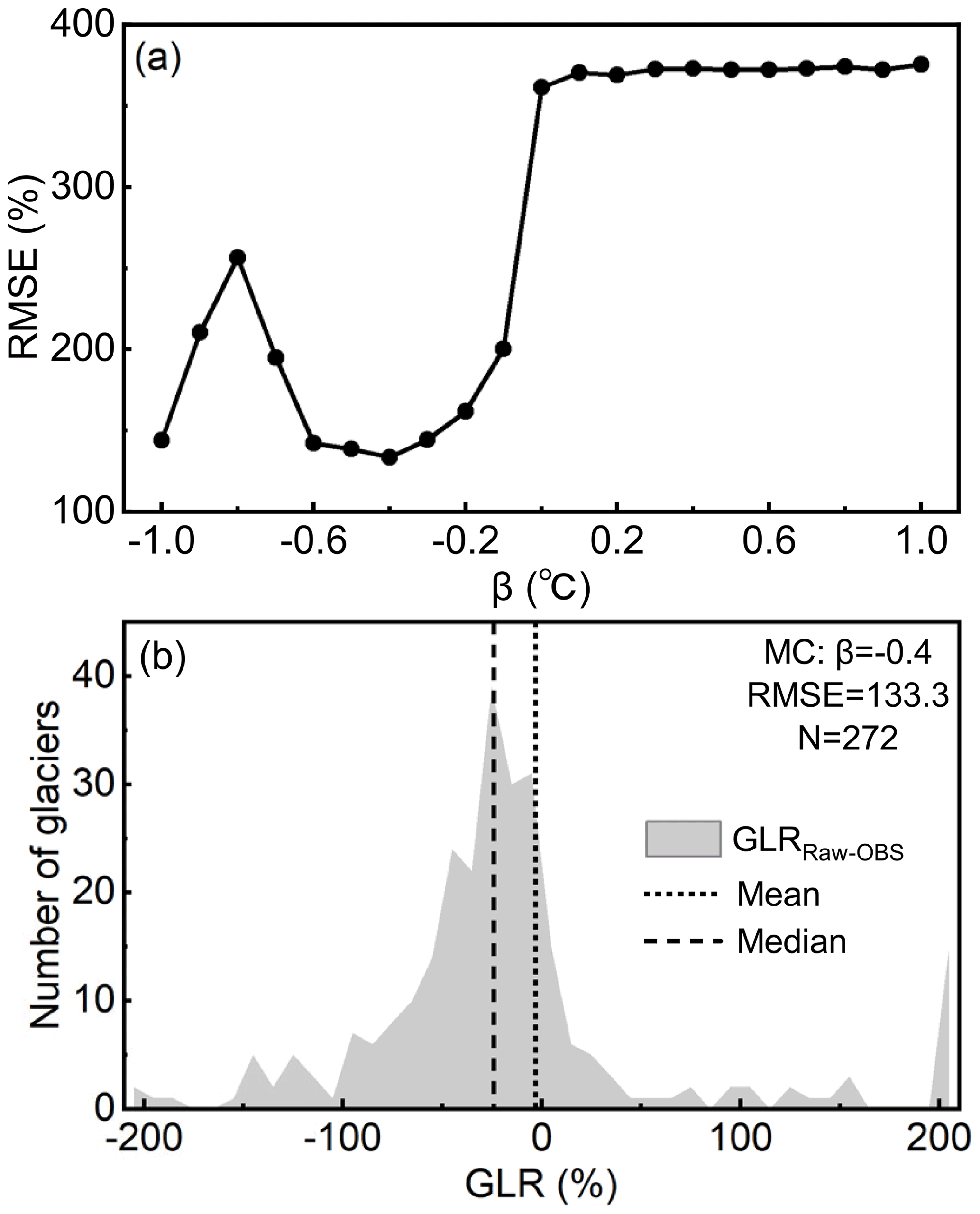
Figure 3(a) The RMSE of maximum peak GLR between the raw simulation results and mapped LIA glaciers for the MC experiment with various β. (b) The simulation bias distribution of maximum peak GLR for the MC experiment with .
3.2 The pattern of glacier changes during the LIA
We focus on the pattern of glacier changes during the LIA in MC experiment, but six GCM simulations are also shown in Fig. 4a for comparison. The simulation results in most experiments indicate four LIA glacial substages in BH, except for the CESM experiment losing the LIA-3 substage. The timings of the four LIA glacial substages are 1270s (LIA-4), 1470s (LIA-3), 1710s (LIA-2), and 1850s (LIA-1) in the MC experiment. These times vary slightly among the six GCM experiments, around the 1230s–1320s, 1470s–1520s, 1620s–1730s, and 1800s–1850s, respectively.
The most extensive glaciers occurred during LIA-4 in MC and six GCM experiments because our tuning strategy is to ensure the larger regional average GLR at the early LIA. The second peak GLR occurred during LIA-1 in the MC experiment. This finding is the same as the results in the CCSM4, GISS, and MPI experiments but different from the results in BCC (LIA-2), CESM (LIA-2), and IPSL (LIA-3) experiments. The third and fourth peak GLR occurred during LIA-3 and LIA-2, respectively, in the MC experiment, which is also consistent with the simulations forced by CCSM4, GISS, and MPI climate datasets.

Figure 4(a) Time series of regional average GLR from 1100 to 1950 CE. (b) The observational timing when glaciers in the monsoonal Himalaya reached their maximum peak GLR. We grouped the moraine ages based on their temporal distances to each glacial substage simulated in the MC experiment. Detailed information on the moraine ages measured by 10Be and 14C can be found in Table S1 and Xu and Yi (2014), respectively.
4.1 Comparison between simulations and observations
We validated the simulation results using the moraine ages across the monsoonal Himalaya and mapped LIA glaciers (Sect. 2.4). The simulated regional average maximum peak GLR (57.4 %; Fig. 3b) in the MC experiment agrees well with that of the mapped glaciers (60.2 %). Similarly, the simulation results in BCC (55.7 %), GISS (54.2 %), and MPI (66.6 %) experiments are also consistent with the observations. Observations from adjacent regions also support the simulation results (Qiao and Yi, 2017; Zhang et al., 2018b). For example, Qiao and Yi (2017) found that the maximum peak GLR increased about 53.8 % during LIA in the central and western Himalayas relative to 2015. Zhang et al. (2018b) reported a 71.5 % increase of maximum peak GLR during LIA in the Gangdise Mountains relative to 2010, based on the glacial geomorphological maps. However, the CCSM4 (89.6 %) and CESM (78.0 %) experiments overestimated the maximum peak GLR, while the IPSL (28.0 %) experiment underestimated it (Fig. S1). In addition, the negative bias for the median value in the simulations compared with observations was identified in the MC and six GCM experiments (Figs. 3b and S1). The difference between the mean value and the median value indicates that some extrema might impact the average.
Based on our tuning strategy (Murari et al., 2014; Xu and Yi, 2014), the maximum peak GLR occurred during LIA-4 in the MC experiment, which was also confirmed by the dated moraine ages in monsoon-influenced Himalaya in that the majority of glaciers advanced to their LIA maximum extents at the early LIA rather than the late LIA (Fig. 4b). Specifically, about 12 of the 30 moraine ages across the monsoonal Himalaya show that the related glaciers reached their maximum peak GLR during LIA-4 compared with only two during LIA-1. However, there is still a large number of glaciers reaching their maximum peak GLR during LIA-3 (about ten glaciers) and LIA-2 (about six glaciers). Ignoring the large uncertainties in the dating methods, the collective and individual differences in glacier changes are worth exploring. We will discuss this issue further in Sect. 4.2.
The simulated number of LIA substages is also comparable with observations, including some moraine dating results and climatic proxy records. For example, Murari et al. (2014) and Zhang et al. (2018a) identified four LIA moraines in the Bhillangana and Dudhganga valleys, Garwal Himalaya, and the Lopu Kangri area, central Gangdise Mountains, respectively. Liu et al. (2017) found at least three LIA moraines in the Lhagoi Kangri Range, Karola Pass. Yang et al. (2003) found four cold phases during AD 1100–1150, 1500–1550, 1650–1700, and 1800–1850 over TP and eastern China according to the proxy data of paleoclimate. A regional moraine chronologies framework composed of 14C, lichenometry and cosmogenic radionuclide ages found three substages during late fourteenth, sixteenth to early eighteenth, and late eighteenth to early nineteenth, corresponding to LIA-3, LIA-2, and LIA-1, respectively (Xu and Yi, 2014). However, the divergent number of LIA substages was also confirmed by some dating results and records. For example, only one moraine was dated in the Cogarbu valley (1484±44 CE; Table S1; Peng et al., 2019) and the Shi Mo valley (1514±69 CE; Table S1; Peng et al., 2020), but two substages were constrained in the Lato valley, Lahul Himalaya (Saha et al., 2018), Langtang Khola valley, Nepal Himalaya (Barnard et al., 2006), and the Gongotri Ganga valley, Garhwal Himalaya (Barnard et al., 2004). By applying dendroglaciology approach, Hochreuther et al. (2015) and Bräuning (2006) only detected one LIA substage in the Gongpu glacier, the Zepu glacier, the Baitong glacier, and the Gyalaperi glacier, while more substages were found in the Lhamcoka glacier (Bräuning, 2006), the Xinpu glacier (Hochreuther et al., 2015), the Gangapurna glacier, and the Annapurna III glacier (Sigdel et al., 2020). Yi et al. (2008) identified three substages during AD 950–1820 based on 53 14C dating ages.
4.2 Why do four LIA substages exist in BH?
Clearly, the MC and GCM experiments (excluding the CESM experiment) indicate four glacial substages over BH during LIA. However, due to the individualities of the glaciers (different slopes and lengths), this does not mean that in each glacier in our study area there exist four LIA substages (Fig. 5a), consistent with the moraine dating results. Instead, it just reflects that the majority of glaciers in BH have four glacial substages. For example, in the MC experiment, only about 33.8 % glaciers have four substages during the LIA, while the remaining glaciers have with zero (4.0 %), one (15.5 %), two (17.9 %), three (26.6 %), and five (2.2 %) substages. We argue that the difference in LIA substages is caused by the sensitivity of different glaciers, even though many studies have ascribed it to the different climate conditions (Owen and Dortch, 2014; Murari et al., 2014; Saha et al., 2019). An analysis found that the number of glacial substages are significantly correlated to the properties of the glacier (length and slope). The number glacial substages has a significantly positive correlation with the glacier slopes and an obviously negative correlation with the glacier length (Fig. 5b and c). The correlation coefficient (CC) between the number of glacial substages and glacier length at 1950 is −0.31, and the CC between the number of glacial substages and glacier slope at 1950 is 0.41. Both of the CCs can pass a 95 % significance test. However, when zooming into the main glacial substages numbers (2, 3, 4), the relationship between the number of glacial substages and the glacier length does not become that clear (Fig. 5b). Therefore, we argue that the glacial slope may dominate the glacial substage numbers during LIA (Lüthi, 2009; Zekollari and Huybrechts, 2015; Bach et al., 2018; Eis et al., 2019). The negative correlation between the glacier length and glacial substage numbers might be a result of the fact that the longer (larger) glacier has a smaller slope (CC = −0.50). Moreover, the analysis also suggests a weak relationship between glacial substage numbers and glacial the equilibrium-line altitude (ELA; Fig. 5d).
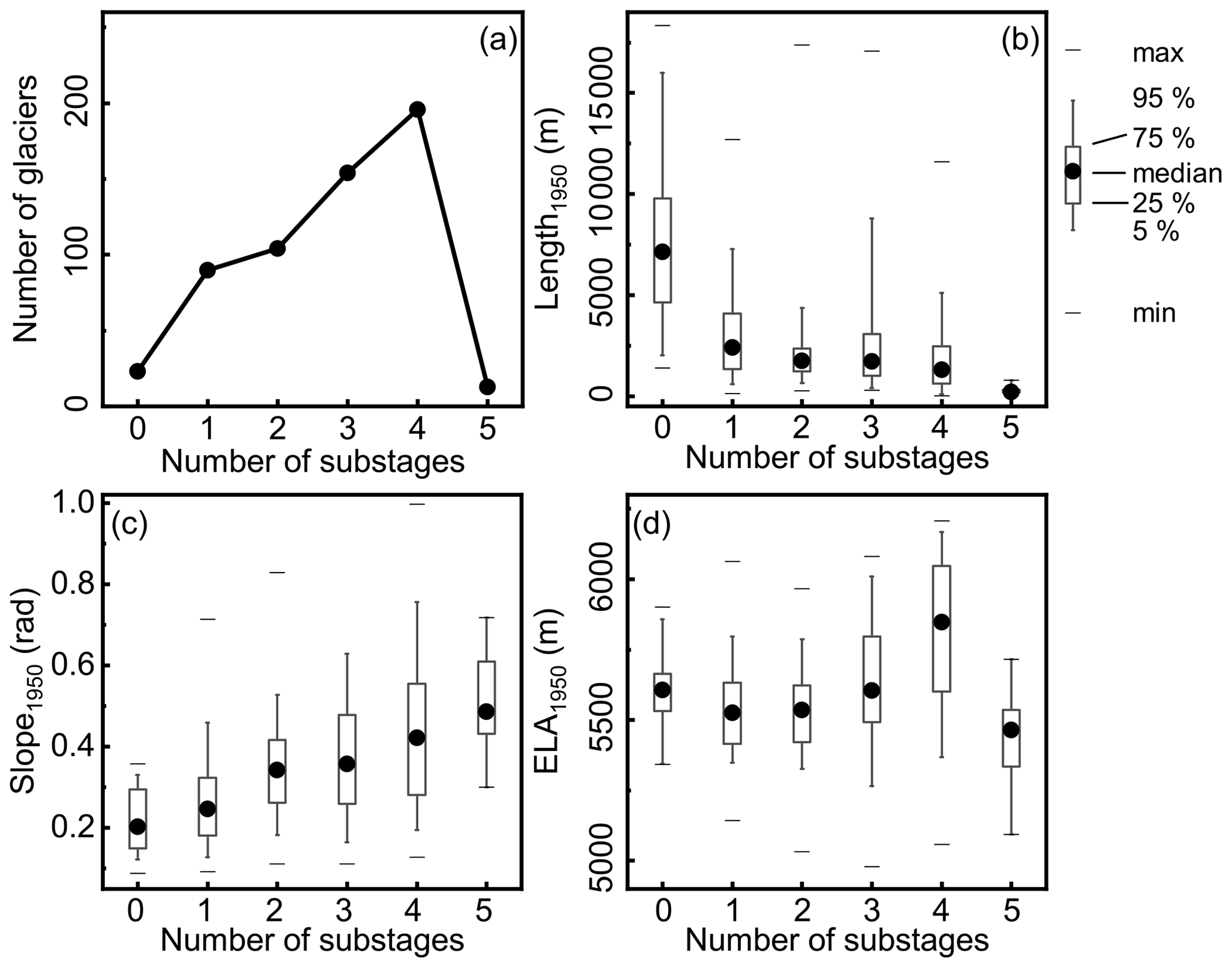
Figure 5(a) The identified glacial substage number distribution in the MC experiment. The relationship between the identified glacial substages with (b) glacier length, (c) glacier slope, and (d) glacial ELA at 1950 in the MC experiment.
The occurrence time of each glacial substage also varies between the glaciers, supported by the dispersal of moraine ages across the monsoonal Himalaya (Fig. 4b). Note that not all glaciers in BH reached their maximum peak GLRs during LIA-4, and taking a step back, even among the glaciers with the maximum peak GLR during LIA-4, the occurrence times were also different (Fig. 6a). Statistically, about 48.1 % of glaciers experienced their maximum peak GLR during LIA-4 followed by 36.1 % of glaciers reaching their maximum peak GLR during LIA-1. Therefore, the occurrence time of maximum peak GLR at regional scale is associated with the occurrence time of the majority of glaciers reaching their maximum peak GLRs. In addition, this can, in turn, explain the lack of some moraines. Considering two glaciers both having four glacial substages but different occurrence times of maximum GLR peak (one at LIA-4 and another at LIA-1) during LIA, we might find four moraines for the glacier that reaches its maximum GLR peak at LIA-4 but only one moraine for the other because the first three moraines are destroyed by the last glacier advance. Similarly, this phenomenon also remains in the occurrence times of the second/third/fourth peak GLR (Fig. 6b–d).
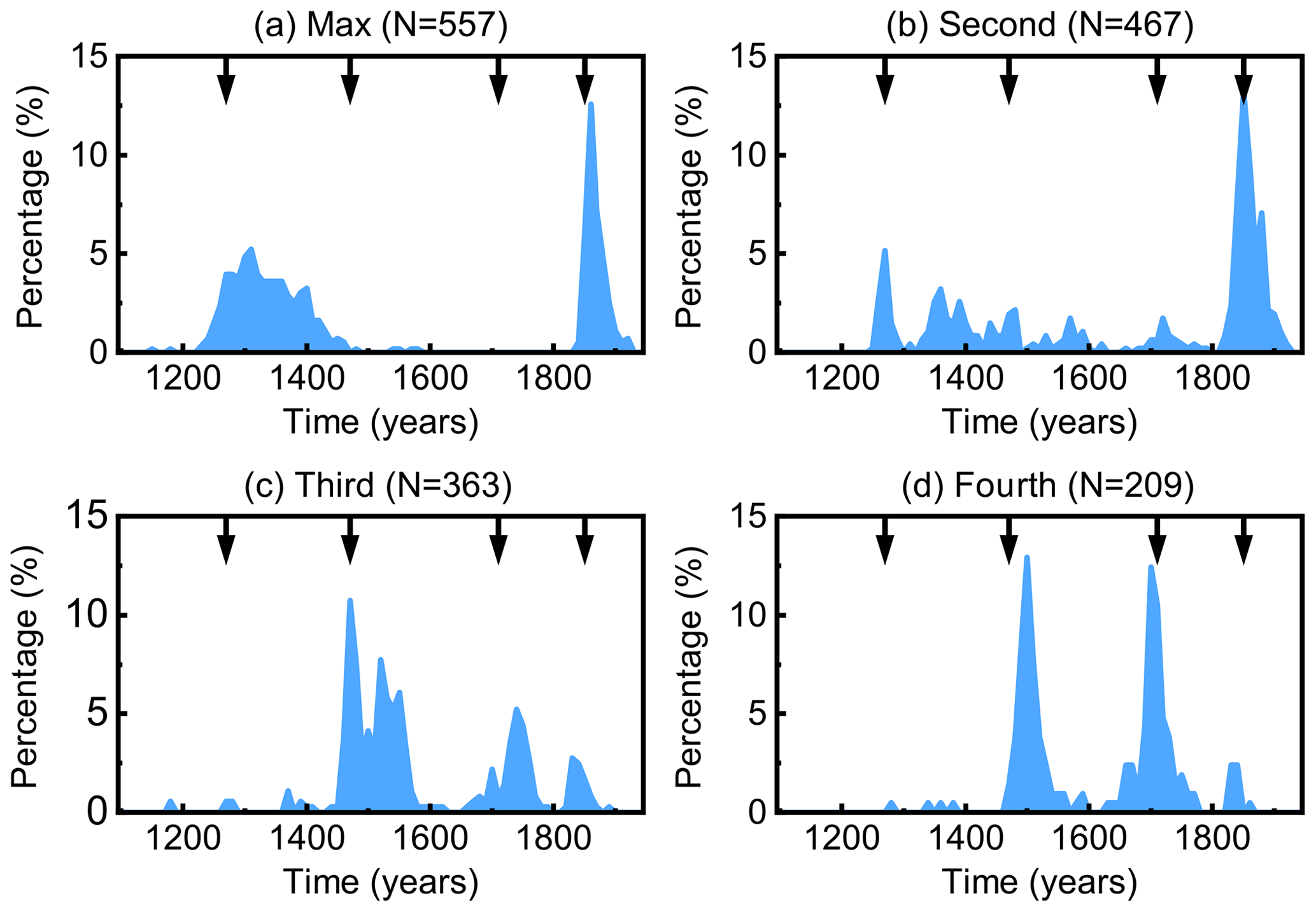
Figure 6Percentage of glaciers with (a) maximum peak GLR, (b) the second largest peak GLR, (c) the third largest peak GLR, and (d) the fourth largest peak GLR over time in the MC experiment. The arrows represent the time of the four glacial substages, the 1270s (LIA-4), 1470s (LIA-3), 1710s (LIA-2), and 1850s (LIA-1).
In summary, four LIA glacial substages during the 1270s, 1470s, 1710s, and 1850s were found in BH based on the MC experiment. The maximum glacier extent appeared during LIA-4, which was confirmed by the moraine ages in the monsoonal influenced Himalaya. The regional glacial evolution is a collective effect of individual glacier changes. Four substages during LIA at the regional scale does not guarantee that each individual glacier has four substages. Likewise, not all glaciers in BH reached their maximum peak GLRs during LIA-4. Instead, it only represents the characteristics of most typical glaciers that accounted for the vast majority of the total glaciers. This can explain why there exist four substages in regional scale in the simulation, but it was difficult to capture in previous studies, which only focussed on one individual glacier. This helps us to thoroughly understand the relationship between regional glacial evolution and the individual glacier response to climate change.
4.3 Climate-forcing mechanisms
The above discussions have explained why there are four glacial substages in BH, but the climatic mechanisms behind these substages described here are still unclear. A better understanding of the possible forcing mechanism of regional paleoglacier fluctuations at centennial timescales benefits projecting glacier outlooks in the future (Solomina et al., 2015). However, due to the limitations of field investigations, previous studies simply ascribed the glacier change to the temperature variation in the monsoon-influenced Himalaya by comparing the regional glacial sequences with the δ18O record from Greenland and the Tibetan or North Atlantic (Peng et al., 2019, 2020). As the model can explicitly link the glacier changes with climate forcings (PDD scheme), which provides us with an opportunity to explore this issue further.
Our study revealed that the regional glacial fluctuations are related to the temperature changes rather than precipitation change (Figs. 4a and 7a, b, d). Four cold intervals around the 1320s, 1510s, 1760s, and 1870s in the MC experiment corresponds to LIA-4 (1270s), LIA-3 (1470s), LIA-2 (1710s), and LIA-1 (1850s), respectively. However, this signal cannot be detected in precipitation changes. Results from six GCM experiments also support this argument, although with different times and strengths. The four cold intervals during the LIA in BH are forced by four large stratospheric sulfur-rich explosive eruptions events (sulfate aerosol loadings >60 Tg; Fig. 7c; Gao et al., 2008), as the volcanic aerosols will inject abundant aerosol into the upper atmosphere, cooling the climate (Schmidt et al., 2012). The beginning of oldest cold period (LIA-4) might have been forced by a series of volcanic activities, including a massive tropical volcanic eruption in 1257, followed by three smaller eruptions in 1268, 1275, and 1284 (Miller et al., 2012). The Billy Mitchell (1580), Huaynaputina (1600), Mount Parker (1641), Long Island (1660), and Laki (1783) volcanoes may have contributed to the cooling events during LIA-3 and LIA-2 (Jonathan, 2007). The 1815 eruption of Tambora and the 1883 eruption of Krakatau are believed to have promoted the youngest cold period of LIA (LIA-1; Rampino and Self, 1982).
Although temperature determines whether BH can run into a glacial substage, precipitation still has the ability to regulate the time of the glacier advancing to its maximum in a glacial substage due to the fact that SMB is determined by the combination of temperature and precipitation, according to the PDD scheme (Eq. 1; Marzeion et al., 2012; Maussion et al., 2019). Positive or negative SMB determines whether a glacier advances or retreats, and the amplitude of glacier change is directly influenced by the amplitude of SMB change and the duration of the positive or negative SMB (Marzeion et al., 2012; Maussion et al., 2019; Figs. 4a and 7e). Four peaks of SMB were found in the MC experiment, around the 1260s, 1460s, 1670s, and 1820s, corresponding to each substage. Stronger precipitation, associated with larger SMB, at the beginning of the cold interval will drive the glacier advance rapidly, shortening the time for it to reach its maximum extent. In addition, we also found that ELA has a good correlation of the SMB, which can be used as a proxy for SMB. ELA is the elevation where accumulation equals ablation for a certain glacier (Fig. 7f; Benn and Lehmkuhl, 2000; Heyman, 2014). Four periods of ELA dropping around the 1270s (−132.2 m), 1470s (−115 m), 1690s (−113.4 m), and 1820s (−112 m) were detected in the MC experiment, agreeing well with SMB change. This finding, to some extent, would benefit field investigations, as paleo ELA is easily available, while paleo SMB is hard to measure.
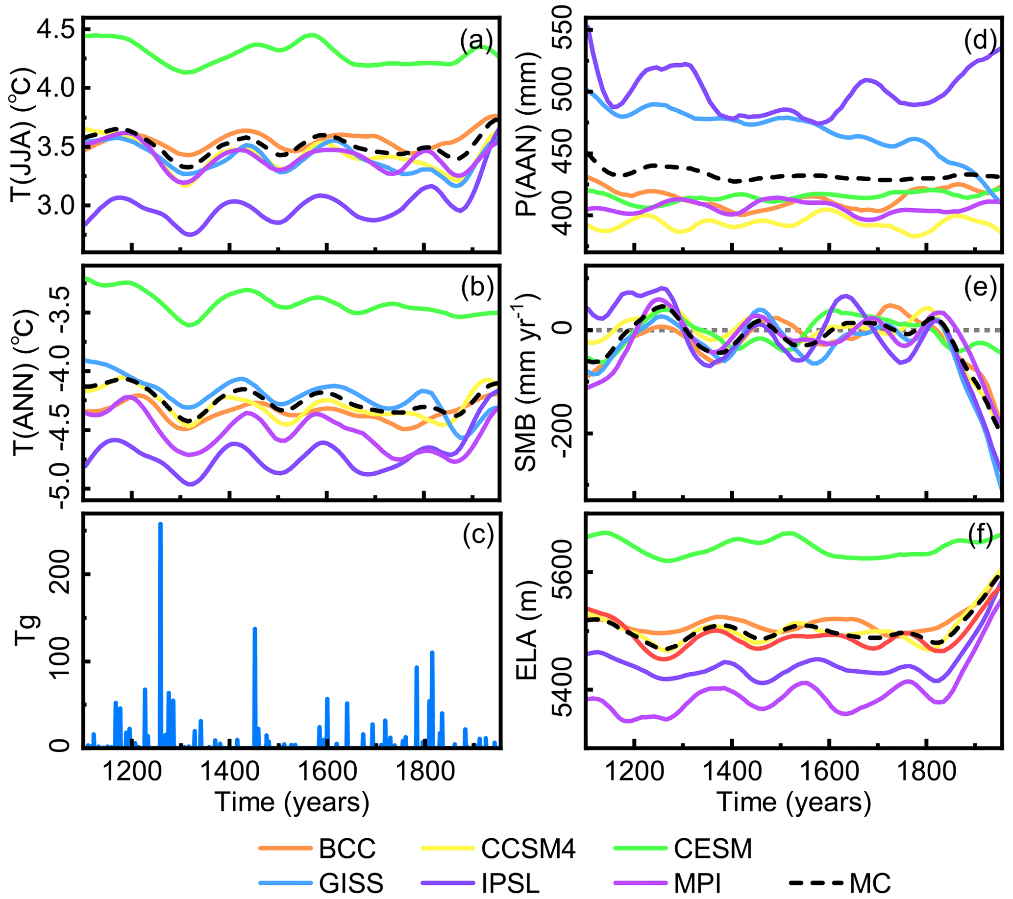
Figure 7The regional average (a) summer temperature (T(JJA)), (b) annual temperature (T(ANN)), (d) annual precipitation (P(ANN)), (e) SMB, (f) ELA from 1100 to 1950 CE at a decadal timescale. (c) Global stratospheric sulfate aerosol loadings (Gao et al., 2008).
The seasonal climate is believed to have a more important impact on glacier evolutions than the annual climate (Yan et al., 2020, 2021). We calculated the regional average monthly temperature, precipitation, cumulative SMB anomalies (relative to the 1950s) from the 1100s to the 1950s (Fig. 8a–c) in the MC experiment to investigate the effect of monthly climate changes on glacial fluctuation. Consistent with Fig. 7e, four significant periods of increase of the monthly SMB changes around the 1270s, 1470s, 1710s, and 1850s are identified (Fig. 8c) as a result of monthly temperature decreases (Fig. 8a). The monthly precipitation does not show any obvious change, expect for an abrupt increase in August (Fig. 8b). The abnormal increase of August precipitation is polluted by the GISS climate dataset, which suffers from large precipitation bias.
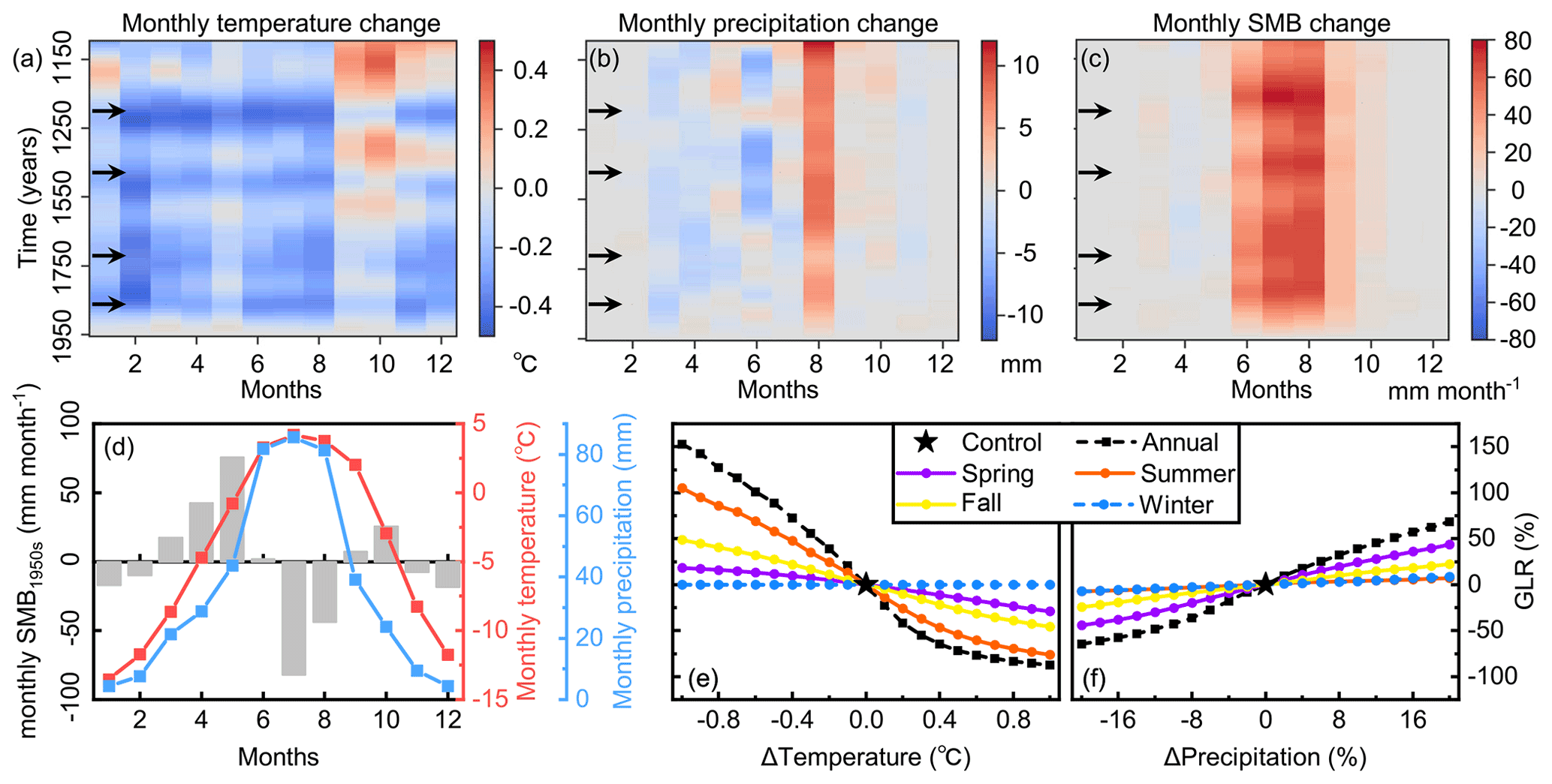
Figure 8The monthly (a) temperature, (b) precipitation, and (c) SMB changes relative to the 1950s at a decadal timescale in the MC experiment. The arrows in (a)–(c) represent the times of the four glacial substages, the 1270s (LIA-4), the 1470s (LIA-3), the 1710s (LIA-2), and the 1850s (LIA-1). (d) The monthly temperature, precipitation, and SMB distribution in the 1950s. Sensitivity of GLR to annual or seasonal (e) temperature and (d) precipitation.
Strong cumulative SMB change only occurs in JJA, despite the fact that the temperature change is distributed almost uniformly and precipitation varies slightly (excluding August) throughout the year. The pattern of seasonal SMB change indicates that the summer temperature might dominate the annual cumulative SMB. This is because JJA is the main ablation season of glaciers in the monsoon-influenced Himalaya due to a higher temperature (Fig. 8d). A reduction of summer temperature will not only decrease the number of positive degree days but also decrease the average temperature during the positive degree days, resulting in the reduction in summer ablation (Eq. 1). Meanwhile, JJA is also the wettest season in the study area. Decreasing temperature will lead to an increasing probability of solid precipitation, enhancing the accumulation. As the SMB is determined by the sum of ablation and the accumulation, the JJA SMB is largely increased. However, although the temperature also decreases in DJF, more precipitation will not increase the accumulation. Therefore, the SMB change is weak.
We also conducted a series of the sensitivity tests to examine the influence of seasonal temperature or precipitation on BH glacier change (Fig. 8e and f). Glaciers retreat gradually as a response to the temperature increases or precipitation decreases. The sensitivity of glaciers to temperature or precipitation changes – in the form of the rate of change for GLR per ∘C or % respectively – is the highest for unmodified temperature or precipitation and decreases as they are varied further from the values given in the historical climate runs. The average GLR changing rates are −160.1 % ∘C−1 and 4.0 % %−1 for annual temperature and precipitation changes, respectively. The maximal sensitivity at unmodified temperature/precipitation is the expected case due to the negative feedback mechanism of changing ELA as glacier length changes. Glaciers are most sensitive to summer temperature changes, with an average change rate of 110.4 % ∘C−1, followed by autumn (51.6 % ∘C−1) and spring (25.2 % ∘C−1). Glaciers are not sensitive to winter temperature changes (0.0 % ∘C−1), which supports the results in Fig. 8c. This indicates that the temperature changes in warm seasons, especially in summer, explain the most variance of GLR changes. Fixing temperature, the sensitivity of glaciers to precipitation changes is higher in spring (2.4 % %−1), followed by autumn (1.1 % %−1), summer (0.4 % %−1), and winter (0.4 % %−1). Therefore, the precipitation changes in spring and autumn has a larger influence on glacier evolution. In order to compare the relative sensitivity of temperature and precipitation to glacier change, we introduced an index , which is a measure of how much precipitation changes in response to temperature changes at present (Jeevanjee and Romps, 2018). This is an index only related to the local climate and is about 1.7 % ∘C−1 in the MC experiment. From our sensitivity tests, we need a k=53.0 % ∘C−1 to maintain the LIA glacier pattern (GLR = 60.6 %), which is much larger than local climate k, indicating that the temperature dominates the LIA glacial fluctuation in BH.
In summary, seasonal analysis and sensitivity tests indicate that the change in temperature, especially summer temperature, is the dominant forcing factor for glacier changes during the LIA (suborbital scale) in monsoonal influenced Himalaya. In contrast, the impact of precipitation change is limited. This conclusion has been drawn by Yan et al. (2020, 2021) at orbital scales but can now be extended to the suborbital scale. In addition, we also found that the temperature changes during LIA are closely related to volcanic activities (Gao et al., 2008; Miller et al., 2012; Schmidt et al., 2012).
We simulated the glacial evolution across BH during LIA using the coupled mass balance and ice flow model, OGGM. Compared with the geomorphological maps and moraine ages, OGGM broadly captures the pattern of glacier length change. The regional pattern of glacier changes is the collective effect of each glacier. The dispersal of the observations could be reproduced by the model due to the individualities of each glacier. On the regional scale, four LIA substages were identified at about the 1270s, 1470s, 1710s, and 1850s (from LIA-4 to LIA-1) in the MC experiment. The most extensive glacial advances occurred during LIA-4, which is consistent with regional glacial chronological and geomorphic evidence. The number of glacial substages for individual glaciers has a positive correlation with glacier slope. The regional glacier advances are dominated by the reduction of summer ablation.
Although limitations still exist in the simulations, such as the application of OGGM on individual glacier changes, this study presented the first simulation of submillennium glacial evolutions during LIA in BH using OGGM. We found a testable relationship between seasonal climate change and glacier expansion, explained the dispersal of moraine ages, and revealed the reasons for the four glacial substages during LIA in BH. Our findings link the limited observations with the model simulations and provides important insights into the climate forcing mechanism on glacier change at the centennial timescale.
Code to run OGGM v1.5.0 is available at https://doi.org/10.5281/zenodo.4765924 (Maussion et al., 2021). The extent of LIA glaciers is available at https://doi.org/10.5281/zenodo.7033379 (Yang et al., 2022). The 10Be surface exposure ages and the related references are listed in the Supplement.
The supplement related to this article is available online at: https://doi.org/10.5194/tc-16-3739-2022-supplement.
Study concept devised by WC. WY performed the model runs and analysis and wrote the original draft. YL and GL reviewed and revised the paper.
The contact author has declared that none of the authors has any competing interests.
Publisher's note: Copernicus Publications remains neutral with regard to jurisdictional claims in published maps and institutional affiliations.
This work was supported by the Second Tibetan Plateau Scientific Expedition and Research (STEP; grant no. 2019QZKK0205) and the National Natural Science Foundation (NSFC; grant nos. 41771005, 41371082). We are grateful to Atle Nesje, Julia Eis, David Parkes, and one anonymous referee for their constructive comments/suggestions that help us a lot to improve the quality of the paper.
This research has been supported by the Second Tibetan Plateau Scientific Expedition and Research (STEP; grant no. 2019QZKK0205) and the National Natural Science Foundation of China, Innovative Research Group Project of the National Natural Science Foundation of China (grant nos. 41771005 and 41371082).
This paper was edited by Ben Marzeion and reviewed by Julia Eis, Atle Nesje, David Parkes, and one anonymous referee.
Bach, E., Radić, V., and Schoof, C.: How sensitive are mountain glaciers to climate change? Insights from a block model, J. Glaciol., 64, 247–258, https://doi.org/10.1017/jog.2018.15, 2018.
Balco, G., Stone, J. O., Lifton, N. A., and Dunai, T. J.: A complete and easily accessible means of calculating surface exposure ages or erosion rates from 10Be and 26Al measurements, Quat. Geochronol., 3, 174–195, https://doi.org/10.1016/j.quageo.2007.12.001, 2008.
Barnard, P. L., Owen, L. A., Sharma, M. C., and Finkel, R. C.: Late Quaternary (Holocene) landscape evolution of a monsoon-influenced high Himalayan valley, Gori Ganga, Nanda Devi, NE Garhwal, Geomorphology, 61, 91–110, https://doi.org/10.1016/j.geomorph.2003.12.002, 2004.
Barnard, P. L., Owen, L. A., Finkel, R. C., and Asahi, K.: Landscape response to deglaciation in a high relief, monsoon-influenced alpine environment, Langtang Himal, Nepal, Quaternary. Sci. Rev., 25, 2162–2176, https://doi.org/10.1016/j.quascirev.2006.02.002, 2006.
Benn, D. I. and Lehmkuhl, F.: Mass balance and equilibrium-line altitudes of glaciers in high-mountain environments, Quatern. Int., 65/66, 15–29, https://doi.org/10.1016/S1040-6182(99)00034-8, 2000.
Bräuning, A.: Tree-ring evidence of “Little Ice Age” glacier advances in southern Tibet, Holocene, 16, 369–380, https://doi.org/10.1191/0959683606hl922rp, 2006.
Bueler, E. and Brown, J.: Shallow shelf approximation as a “sliding law” in a thermo mechanically coupled ice sheet model, J. Geophys. Res-Earth., 114, F03008, https://doi.org/10.1029/2008JF001179, 2009.
Carrivick, J. L., Boston, C. M., King, W., James, W. H., Quincey, D. J., Smith, M. W., Grimes, M., and Evans, J.: Accelerated volume loss in glacier ablation zones of NE Greenland, Little Ice Age to present, Geophys. Res. Lett., 46, 1476–1484, https://doi.org/10.1029/2018GL081383, 2019.
Chandler, B. M. P., Boston, C. M., and Lukas, S.: A spatially-restricted Younger Dryas plateau icefield in the Gaick, Scotland: Reconstruction and palaeoclimatic implications, Quaternary. Sci. Rev., 211, 107–135, https://doi.org/10.1016/j.quascirev.2019.03.019, 2019.
Chen, W., Yao, T., Zhang, G., Li, F., Zheng, G., Zhou, Y., and Xu, F.: Towards ice-thickness inversion: an evaluation of global digital elevation models (DEMs) in the glacierized Tibetan Plateau, The Cryosphere, 16, 197–218, https://doi.org/10.5194/tc-16-197-2022, 2022.
Chevalier, M.-L., Hilley, G., Tapponnier, P., Woerd, J. V. D., Liu-Zeng, J., Finkel, R. C., Ryerson, F. J., Li, H., and Liu, X.: Constraints on the late Quaternary glaciations in Tibet from cosmogenic exposure ages of moraine ages, Quaternary. Sci. Rev., 30, 528–554, https://doi.org/10.1016/j.quascirev.2010.11.005, 2011.
Dixit, A., Sahany, S., and Kulkarni, A. V.: Glacial changes over the Himalayan Beas basin under global warming, J. Environ. Manage., 295, 113101, https://doi.org/10.1016/j.jenvman.2021.113101, 2021.
Dong, G., Zhou, W., Yi, C., Fu, Y., Zhang, L., and Li, M.: The timing and cause of glacial activity during the last glacial in central Tibet based on 10Be surface exposure dating east of Mount Jagang, the Xianza range, Quaternary. Sci. Rev., 186, 284–297, https://doi.org/10.1016/j.quascirev.2018.03.007, 2018.
Dortch, J. M., Owen, L. A., and Caffee, M. W.: Timing and climatic drivers for glaciation across semi-arid western Himalayan-Tibetan orogen, Quaternary. Sci. Rev., 78, 188–208, https://doi.org/10.1016/j.quascirev.2013.07.025, 2013.
Eis, J., Maussion, F., and Marzeion, B.: Initialization of a global glacier model based on present-day glacier geometry and past climate information: an ensemble approach, The Cryosphere, 13, 3317–3335, https://doi.org/10.5194/tc-13-3317-2019, 2019.
Farinotti, D., Brinkerhoff, D. J., Clarke, G. K. C., Fürst, J. J., Frey, H., Gantayat, P., Gillet-Chaulet, F., Girard, C., Huss, M., Leclercq, P. W., Linsbauer, A., Machguth, H., Martin, C., Maussion, F., Morlighem, M., Mosbeux, C., Pandit, A., Portmann, A., Rabatel, A., Ramsankaran, R., Reerink, T. J., Sanchez, O., Stentoft, P. A., Singh Kumari, S., van Pelt, W. J. J., Anderson, B., Benham, T., Binder, D., Dowdeswell, J. A., Fischer, A., Helfricht, K., Kutuzov, S., Lavrentiev, I., McNabb, R., Gudmundsson, G. H., Li, H., and Andreassen, L. M.: How accurate are estimates of glacier ice thickness? Results from ITMIX, the Ice Thickness Models Intercomparison eXperiment, The Cryosphere, 11, 949–970, https://doi.org/10.5194/tc-11-949-2017, 2017.
Farinotti, D., Huss, M., Fürst, J. J., Landmann, J., Machguth, H., Maussion, F., and Pandit, A.: A consensus estimate for the ice thickness distribution of all glaciers on Earth, Nat. Geosci., 12, 168–173, https://doi.org/10.1038/s41561-019-0300-3, 2019.
Fu, P., Stroeven, A. P., Harbor, J. M., Hättestrand, C., Heyman, J., Caffee, M. W., and Zhou, P.: Paleoglaciation of Shaluli Shan, southeastern Tibetan Plateau, Quaternary. Sci. Rev., 64, 121–135, https://doi.org/10.1016/j.quascirev.2012.12.009, 2013.
Furian, W., Maussion, F., and Schneider, C.: Projected 21st-Century Glacial Lake Evolution in High Moutain Asia, Front. Earth. Sci., 10, 821798, https://doi.org/10.3389/feart.2022.821798, 2022.
Gao, C., Robock, A., and Ammann, C.: Volcanic forcing of climate over the past 1500 years: An improved ice core-based index for climate models, J. Geophys. Res., 113, D23111, https://doi.org/10.1029/2008JD010239, 2008.
Goosse, H., Barriat, P.-Y., Dalaiden, Q., Klein, F., Marzeion, B., Maussion, F., Pelucchi, P., and Vlug, A.: Testing the consistency between changes in simulated climate and Alpine glacier length over the past millennium, Clim. Past, 14, 1119–1133, https://doi.org/10.5194/cp-14-1119-2018, 2018.
Greve, R.: A continuum-mechanical formulation for shallow polythermal ice sheets, Philos. T.R. Soc. A., 355, 921–974, https://doi.org/10.1175/1520-0442(1997)010<0901:AOAPTD>2.0.CO;2, 1997a.
Greve, R.: Application of a polythermal three-dimensional ice sheet model to the Greenland ice sheet: Response to steady-state and transient climate scenarios, J. Climate, 10, 901–918, https://doi.org/10.1098/rsta.1997.0050, 1997b.
Grove, J. M.: Little Ice Age, 2 edn., Routledge, https://doi.org/10.4324/9780203402863, 2013.
Harris, I., Osborn, T. J., Jones, P., and Lister, D.: Version 4 of the CRU TS monthly high-resolution gridded multivariate climate dataset, Sci. Data, 7, 109, 109, https://doi.org/10.1038/s41597-020-0453-3, 2020.
Heyman, J.: Paleoglaciation of the Tibetan Plateau and surrounding mountains based on exposure ages and ELA depression estimates, Quaternary. Sci. Rev., 91, 30–41, https://doi.org/10.1016/j.quascirev.2014.03.018, 2014.
Heyman, J., Stroeven, A. P., Harbor, J. M., and Caffee, M. W.: Too young or too old: Evaluating cosmogenic exposure dating based on an analysis of compiled boulder exposure ages, Earth. Planet. Sc. Lett., 302, 71–80, https://doi.org/10.1016/j.epsl.2010.11.040, 2011.
Hochreuther, P., Loibl, D., Wernicke, J., Zhu, H., Grießinger, J., and Bräuning, A.: Ages of major Little Ice Age glacier fluctuations on the southeast Tibetan Plateau derived from tree-ring-based moraine dating, Palaeogeogr. Palaeocl., 422, 1–10, https://doi.org/10.1016/j.palaeo.2015.01.002, 2015.
Jarvis, A., Reuter, H., Nelson, A., and Guevara, E.: Hole-filledSRTM for the globe Version 4, CGIAR Consortium for Spatial Inf ormation, University of Twente, 2008.
Jeevanjee, N. and Romps, D. M.: Mean precipitation change from a deepening troposphere, P. Natl. Acad. Sci. USA, 115, 11465–11470, https://doi.org/10.1073/pnas.1720683115, 2018.
Jonathan, C.: Climate change: biological and human aspects, Cambridge University Press, 164, ISBN 978-0-521-69619-7, 2007.
Lifton, N., Sato, T., and Dunai, T. J.: Scaling in situ cosmogenic nuclide production rates using analytical approximations to atmospheric cosmic-ray fluxes, Earth. Planet. Sc. Lett., 386, 149–160, https://doi.org/10.1016/j.epsl.2013.10.052, 2014.
Lipscomb, W. H., Price, S. F., Hoffman, M. J., Leguy, G. R., Bennett, A. R., Bradley, S. L., Evans, K. J., Fyke, J. G., Kennedy, J. H., Perego, M., Ranken, D. M., Sacks, W. J., Salinger, A. G., Vargo, L. J., and Worley, P. H.: Description and evaluation of the Community Ice Sheet Model (CISM) v2.1, Geosci. Model Dev., 12, 387–424, https://doi.org/10.5194/gmd-12-387-2019, 2019.
Liu, J., Yi, C., Li, Y., Bi, W., Zhang, Q., and Hu, G.: Glacial fluctuations around the Karola Pass, eastern Lhagoi Kangri Range, since the Last Glacial Maximum, J. Quaternary. Sci., 32, 516–527, https://doi.org/10.1002/jqs.2946, 2017.
Lüthi, M. P.: Transient response of idealized glaciers to climate variations, J. Glaciol., 55, 918–903, https://doi.org/10.3189/002214309790152519, 2009.
Marzeion, B., Jarosch, A. H., and Hofer, M.: Past and future sea-level change from the surface mass balance of glaciers, The Cryosphere, 6, 1295–1322, https://doi.org/10.5194/tc-6-1295-2012, 2012.
Maussion, F., Butenko, A., Champollion, N., Dusch, M., Eis, J., Fourteau, K., Gregor, P., Jarosch, A. H., Landmann, J., Oesterle, F., Recinos, B., Rothenpieler, T., Vlug, A., Wild, C. T., and Marzeion, B.: The Open Global Glacier Model (OGGM) v1.1, Geosci. Model Dev., 12, 909–931, https://doi.org/10.5194/gmd-12-909-2019, 2019.
Maussion, F., Roth, T., Dusch, M., Recinos, B., Vlug, A., Champollion, N., Marzeion, B., Schuster, L., Oberrauch, M., Landmann, J., Eis, J.,Jarosch, A., sarah-hanus, Li, F., Rounce, D., Castellani, M., Bartholomew, S. L., Merrill, C., Loibl, D., Ultee, L., Smith, S., anton-ub, and Gregor, P.: OGGM/oggm: v1.5.0 (v1.5.0), Zenodo [code], https://doi.org/10.5281/zenodo.4765924, 2021.
Miller, G. H., Geirsdttir, Á., Zhong, Y., Larsen, D. J., Otto-Bliesner, B. L., Holland, M. M., Bailey, D. A., Refsnider, K. A., Lehman, S. J., Southon, J. R., Anderson, C., Björnsson, H., and Thordarson, T.: Abrupt onse of the Little Ice Age triggered by volcanism and sustained by sea-ice/ocean feedbacks, Geophys. Res. Lett., 39, L02708, https://doi.org/10.1029/2011GL050168, 2012.
Murari, M. K., Owen, L. A., Dortch, J. M., Caffee, M. W., Dietsch, C., Fuchs, M., Haneberg, W. C., Sharma, M. C., and Townsend-Small, A.: Timing and climatic drivers for glaciation across monsoon-influenced regions of the HimalayaneTibetan orogen, Quaternary. Sci. Rev., 88, 159–182, https://doi.org/10.1016/j.quascirev.2014.01.013, 2014.
Oerlemans, J., Anderson, B., Hubbard, A., Huybrechts, Ph., Jóhannesson, T., Knap, W. H., Schmeits, M., Stroeven, A. P., van de Wal, R. S. W., and Zuo, Z.: Modelling the response of glaciers to climate warming, Clim. Dynam., 14, 267–274, https://doi.org/10.1007/s003820050222, 1998.
Owen, L. A.: Latest Pleistocene and Holocene glacier fluctuations in the Himalaya and Tibet, Quaternary. Sci. Rev., 28, 2150–2164, https://doi.org/10.1016/j.quascirev.2008.10.020, 2009.
Owen, L. A. and Dortch, J. M.: Nature and timing of Quaternary glaciation in the Himalayan-Tibetan orogen, Quaternary. Sci. Rev., 88, 14–54, https://doi.org/10.1016/j.quascirev.2013.11.016, 2014.
PAGES 2k-PMIP3 group: Continental-scale temperature variability in PMIP3 simulations and PAGES 2k regional temperature reconstructions over the past millennium, Clim. Past, 11, 1673–1699, https://doi.org/10.5194/cp-11-1673-2015, 2015.
Parkes, D. and Goosse, H.: Modelling regional glacier length changes over the last millennium using the Open Global Glacier Model, The Cryosphere, 14, 3135–3153, https://doi.org/10.5194/tc-14-3135-2020, 2020.
Pelto, B. M., Maussion, F., Menounos, B., Radić, V., and Zeuner, M.: Bias-corrected estimates of glacier thickness in the Columbia River Basin, Canada, J. Glaciol., 66, 1051–1063, https://doi.org/10.1017/jog.2020.75, 2020.
Peng, X., Chen Y., Liu, G., Liu, B., Li, Y., Liu, Q., Han, Y., Yang, W., and Cui, Z.: Late Quaternary glaciations in the Cogarbu valley, Bhutanese Himalaya, J. Quaternary. Sci., 34, 40–50, https://doi.org/10.1002/jqs.3079, 2019.
Peng, X., Chen, Y., Li, Y., Liu, B., Liu, Q., Yang, W., and Liu, G.: Late Holocene glacier fluctuations in the Bhutanese Himalaya, Global. Planet. Change, 187, 103137, https://doi.org/10.1016/j.gloplacha.2020.103137, 2020.
Pronk, J. B., Bolch, T., King, O., Wouters, B., and Benn, D. I.: Contrasting surface velocities between lake- and land-terminating glaciers in the Himalayan region, The Cryosphere, 15, 5577–5599, https://doi.org/10.5194/tc-15-5577-2021, 2021.
Qiao, B. and Yi, C.: Reconstruction of Little Ice Age glacier area and equilibrium line attitudes in the central and western Himalaya, Quatern. Int., 444, 65–75, https://doi.org/10.1016/j.quaint.2016.11.049, 2017.
Qureshi, M. A., Li, Y., Yi, C., and Xu, X.: Glacial changes in the Hunza Basin, western Karakoram, since the Little Ice Age, Palaeogeogr. Palaeocl., 562, 110086, https://doi.org/10.1016/j.palaeo.2020.110086, 2021.
Rampino, M. R. and Self, S.: Historic Eruptions of Tambora (1815), Krakatau (1883), and Agung (1963), their Stratospheric Aerosols, and Climatic Impact, Quatern. Res., 18, 127–143, https://doi.org/10.1016/0033-5894(82)90065-5, 1982.
RGI Consortium: Randolph Glacier Inventory (RGI)-A Dataset of Global Glacier Outlines: Version 6.0, https://doi.org/10.7265/N5-RGI-60, 2017.
Saha, S., Owen, L. A., Orr, E. N., and Caffee, M. W.: Timing and nature of Holocene glacier advances at the northwestern end of the Himalayan-Tibetan orogen, Quaternary. Sci. Rev., 187, 177–202, https://doi.org/10.1016/j.quascirev.2018.03.009, 2018.
Saha, S., Owen, L. A., Orr, E. N., and Caffee, M. W.: High-frequency Holocene glacier fluctuations in the Himalayan-Tibetan orogen, Quaternary Sci. Rev., 220, 372–400, https://doi.org/10.1016/j.quascirev.2019.07.021, 2019.
Schmidt, G. A., Jungclaus, J. H., Ammann, C. M., Bard, E., Braconnot, P., Crowley, T. J., Delaygue, G., Joos, F., Krivova, N. A., Muscheler, R., Otto-Bliesner, B. L., Pongratz, J., Shindell, D. T., Solanki, S. K., Steinhilber, F., and Vieira, L. E. A.: Climate forcing reconstructions for use in PMIP simulations of the last millennium (v1.0), Geosci. Model Dev., 4, 33–45, https://doi.org/10.5194/gmd-4-33-2011, 2011.
Shafeeque, M. and Luo, Y.: A multi-perspective approach for selecting CMIP6 scenarios to project climate change impacts on glacio-hydrology with a case study in Upper Indus River basin, J. Hydrol., 599, 126466, https://doi.org/10.1016/j.jhydrol.2021.126466, 2021.
Sigdel, S.R., Zhang, H., Zhu, H., Muhammad, S., and Liang, E.: Retreating glacier and advancing forest over the past 200 years in the Central Himalayas, J. Biogeogr., 125, e2020JG005751. https://doi.org/10.1029/2020JG005751, 2020.
Solomina, O. N., Bradley, R. S., Hodgson, D. A., Ivy-Ochs, S., Jomelli, V., Mackintosh, A. N., Nesje, A., Owen, L. A., Wanner, H., Wiles, G. C., and Young, N. E.: Holocene glacier fluctuations, Quaternary. Sci. Rev., 111, 9–34, https://doi.org/10.1016/j.quascirev.2014.11.018, 2015.
Taylor, K., Stouffer, R., and Meehl, G.: An Overview of CMIP5 and the Experiment Design, B. Am. Meteorol. Soc., 93, 485–498, https://doi.org/10.1175/BAMS-D-11-00094.1, 2012.
WGMS: Fluctuations of Glaciers Database, World Glacier Monitoring Service, Zurich, Switzerland, https://doi.org/10.5904/wgms-fog-2021-05, 2021.
Winkelmann, R., Martin, M. A., Haseloff, M., Albrecht, T., Bueler, E., Khroulev, C., and Levermann, A.: The Potsdam Parallel Ice Sheet Model (PISM-PIK) – Part 1: Model description, The Cryosphere, 5, 715–726, https://doi.org/10.5194/tc-5-715-2011, 2011.
Xu, X. and Yi, C.: Little Ice Age on the Tibetan Plateau and its bordering mountains: Evidence from moraine chronologies, Global. Planet. Change., 116, 41–53, https://doi.org/10.1016/j.gloplacha.2014.02.003, 2014.
Yan, Q., Owen, L. A., Wang, H., and Zhang, Z.: Climate constraints on glaciation over High-Mountain Asia during the last glacial maximum, Geophys. Res. Lett., 45, 9024–9033, https://doi.org/10.1029/2018GL079168, 2018.
Yan, Q., Owen, L. A., Zhang, Z., Jiang, N., and Zhang, R.: Deciphering the evolution and forcing mechanisms of glaciation over the Himalayan-Tibetan orogen during the past 20,000 years, Earth. Planet. Sc. Lett., 541, 116295, https://doi.org/10.1016/j.epsl.2020.116295, 2020.
Yan, Q., Owen, L. A., Zhang, Z., Wang, H., Wei, T., Jiang, N., and Zhang, R.: Divergent evolution of glaciation across High-Mountain Asia during the last four glacial-interglacial cycles, Geophys. Res. Lett., 48, e2021GL092411, https://doi.org/10.1029/2021GL092411, 2021.
Yang, B., Achim, B., and Shi, Y.: Late Holocene temperature fluctuations on the Tibetan Plateau, Quaternary. Sci. Rev., 22, 2335–2344, https://doi.org/10.1016/S0277-3791(03)00132-X, 2003.
Yang, W., Li, Y., Liu, G., and Chu, W.: Mapped glacier region in BH during LIA, Zenodo [data set], https://doi.org/10.5281/zenodo.7033379, 2022.
Yi, C., Chen, H., Yang, J., Liu, B., Fu, P., Liu, K., and Li, S.: Review of Holocene glacial chronologies based on radiocarbon dating in Tibet and its surrounding mountains, J. Quaternary. Sci., 23, 533–543, https://doi.org/10.1002/jqs.1228, 2008.
Zekollari, H. and Huybrechts, P.: On the climate–geometry imbalance, response time and volume–area scaling of an alpine glacier: insights from a 3-D flow model applied to Vadret da Morteratsch, Switzerland, Ann. Glaciol., 56, 51–62, https://doi.org/10.3189/2015AoG70A921, 2015.
Zhang, Q., Yi, C., Dong, G., Fu, P., Wang, N., and Capolongo, D.: Quaternary glaciations in the Lopu Kangri area, central Gangdise Mountains, southern Tibetan Plateau, Quaternary. Sci. Rev., 201, 470–482, https://doi.org/10.1016/j.quascirev.2018.10.027, 2018a.
Zhang, Q., Yi, C., Fu, P., Wu, Y., Liu, J., and Wang, N.: Glacier change in the Gangdise Mountains, southern Tibet, since the Little Ice Age, Geomorphology, 306, 51–63, https://doi.org/10.1016/j.geomorph.2018.01.002, 2018b.