the Creative Commons Attribution 4.0 License.
the Creative Commons Attribution 4.0 License.
 | 09 Sep 2022
High-resolution imaging of supraglacial hydrological features on the Greenland Ice Sheet with NASA's Airborne Topographic Mapper (ATM) instrument suite
Michael Studinger
Serdar S. Manizade
Matthew A. Linkswiler
James K. Yungel
Seasonal meltwater pools on the surface of the Greenland Ice Sheet (GrIS) during late spring and summer in lakes on the surface and transforms the ice sheet's surface into a wet environment in the ablation zone below the equilibrium line. These supraglacial lakes in topographic lows on the ice surface are connected by a dendritic pattern of meandering streams and channels that together form a hydrological system consisting of supra-, en-, and subglacial components. Here, we use lidar data from NASA's Airborne Topographic Mapper (ATM) instrument suite and high-resolution optical imagery collected as part of Operation IceBridge (OIB) in spring 2019 over the GrIS to develop methods for the study of supraglacial hydrological features. While airborne surveys have a limited temporal and spatial coverage compared to imaging spaceborne sensors, their high footprint density and high-resolution imagery reveal a level of detail that is currently not obtainable from spaceborne measurements. The accuracy and resolution of airborne measurements complement spaceborne measurements, can support calibration and validation of spaceborne methods, and provide information necessary for high-resolution process studies of the supraglacial hydrological system on the GrIS that currently cannot be achieved from spaceborne observations alone.
- Article
(17022 KB) - Full-text XML
- BibTeX
- EndNote


During the summer months, seasonal surface melting on the Greenland Ice Sheet (GrIS) produces meltwater near the margins of the ice sheet that pools in supraglacial lakes in depressions on the ice surface and forms a dendritic pattern of meandering streams and rivers in the ablation zone below the equilibrium line (e.g., Chu, 2014; Nienow et al., 2017; Pitcher and Smith, 2019, and references therein). The lakes appear as sapphire-blue features to the eye and in natural color imagery (Flowers, 2018) (Fig. 1). The supraglacial streams and channels often connect several lakes and form a hydrological network on the surface of the GrIS that is part of a hydrological system consisting of supra-, en-, and subglacial components (e.g., Chu, 2014; Nienow et al., 2017; Pitcher and Smith, 2019, and references therein). The formation, retention, and drainage of meltwater impacts ice sheet mass balance and therefore ice sheet stability. Over the past decades, runoff from seasonal meltwater production has exceeded ice loss from ice discharge and basal melting at the grounding lines and has become the dominant mechanism of mass loss for the GrIS (Enderlin et al., 2014; van den Broeke et al., 2016). More recently, supraglacial lakes and channels have also been catalogued on the West Antarctic Ice Sheet (Corr et al., 2022).
Several approaches have been used in recent years to study the supraglacial hydrological network of lakes and streams at various spatial and temporal scales. On an ice-sheet-wide scale, the network of supraglacial hydrological features and their temporal evolution can be observed with panchromatic, natural color, and multi-spectral imagery available from multiple satellite missions at various spatial resolutions (e.g., Box and Ski, 2007; Pope et al., 2016; Sneed and Hamilton, 2007, 2011; Yang and Smith, 2016; Yang et al., 2017, and references therein). Pixel-based surface classification of satellite imagery is a powerful tool for identifying and mapping networks of supraglacial lakes and streams; however, challenges remain with precise spatial registration of repeat high-resolution imagery (e.g., Yang et al., 2017). Estimating water depths from satellite imagery based on reflectance–depth relationships (i.e., optical depth) requires either natural color or multi-spectral imagery (e.g., Pope et al., 2016). Sneed and Hamilton (2011) list several simplifying assumptions necessary for optical depth-based estimates including a homogenous and smooth lake surface without any wind-induced waves and a homogenous lake bottom that is roughly parallel to the lake surface. As shown later in this paper (Fig. 7a) surface waves are not uncommon, and an oblique aerial photograph of a supraglacial lake shows that newly formed thin ice and snow-covered lake ice further complicate depth estimates based on reflectance (Fig. 1). The photograph also shows a complex lake bottom topography and reflectance that is far from homogenous. Dark lake bottom sediments in the form of cryoconite, as well as meltwater channels and bottom crevasses, can be seen complicating the analysis, although Pope et al. (2016) developed a method that accounts for the presence of cryoconite. Yang and Smith (2013) emphasize the need to gain a better understanding of supraglacial streams, which is limited due to supraglacial streams' relatively narrow width (∼ 1–30 m) making detection difficult using moderate-resolution satellite imagery. However, the recent increase in availability of high-resolution satellite imagery shows improvements in our knowledge of supraglacial streams (Yang and Smith, 2013). Whereas small-scale streams, several meters wide, can be detected with high-resolution satellite imagery, determining their depths from spaceborne measurements remains difficult (Flowers, 2018).

Figure 1Oblique aerial photograph of a supraglacial lake (approximate location 67∘12′38′′ N, 49∘54′46′′ W) on Isunnguata Sermia near Kangerlussuaq from 13 May 2019 (photo: Michael Studinger). The lake is approximately 280 m wide. For location see Fig. 2. Surface temperature and surface melt indicator from the Moderate Resolution Imaging Spectroradiometer (MODIS) (Hall et al., 2018; Hall and DiGirolamo, 2019), as well as number of melt days for this location, are shown in Fig. A1a.
On a local scale, remotely controlled drone boats and zodiacs equipped with spectroradiometers, digital fathometers, and sonars have been used to measure spectral properties of lakes and streams for calibration and validation of depth estimates based on satellite imagery, as well as directly measure water depth (e.g., Box and Ski, 2007; Das et al., 2008; Legleiter et al., 2014; Pope et al., 2016; Smith et al., 2017; Tedesco and Steiner, 2011).
More recently, spaceborne and airborne lidars have been used to estimate lake depths (Datta and Wouters, 2021; Fair et al., 2020). Airborne measurements can map supraglacial hydrological features on the GrIS at a level of detail that can currently not be accomplished by spaceborne instruments. Airborne measurements can also map supraglacial hydrological features at a spatial scale that cannot be achieved by measurements from short-range drones operated out of remote field camps that often require line-of-sight communication. More detailed studies of the supraglacial fluvial system on the GrIS are needed (Smith et al., 2015, p. 1001). Here, we use airborne laser altimetry and high-resolution optical imagery collected as part of Operation IceBridge (OIB) in spring 2019 over the GrIS (MacGregor et al., 2021) to develop methods that allow the study of the bathymetry of supraglacial hydrological features currently not possible from space or on the ground.
OIB campaigns were scheduled to survey the sea ice maximum in March and survey the GrIS at the end of the winter season in early spring when ice temperatures are still cold to optimize penetration and quality of the ice-penetrating radar data (MacGregor et al., 2021). As a result of this data acquisition strategy, some of the campaigns barely captured the early onset of the summer melt in central and southern Greenland but did not capture the peak of the melt season. In addition to the spring campaigns, several “summer campaigns” have been flown at the end of the Arctic summer to capture the extent of the summer melt. Because of the timing of these campaigns, temperatures were often below freezing and most of the supraglacial hydrological features were already frozen over. Figure A1 shows the daily mean surface temperature from the Moderate Resolution Imaging Spectroradiometer (MODIS) and the surface melt indicator for the locations of the lakes and channels shown in Figs. 1 and 7–9 (Hall et al., 2018; Hall and DiGirolamo, 2019). We analyze nine flights from OIB's 2019 Arctic spring campaign between 5 and 16 May 2019. We also analyzed four flights of the Arctic fall campaign between 10 and 14 September 2019 which cover the region where supraglacial hydrological features in the spring campaign are present (Fig. 2). The four flights in September 2019 did not conclusively show the presence of liquid water surfaces, and therefore no examples of those flights are discussed in this paper, which primarily focuses on method development. All airborne data used in this study are freely available at the National Snow and Ice Data Center (NSIDC).
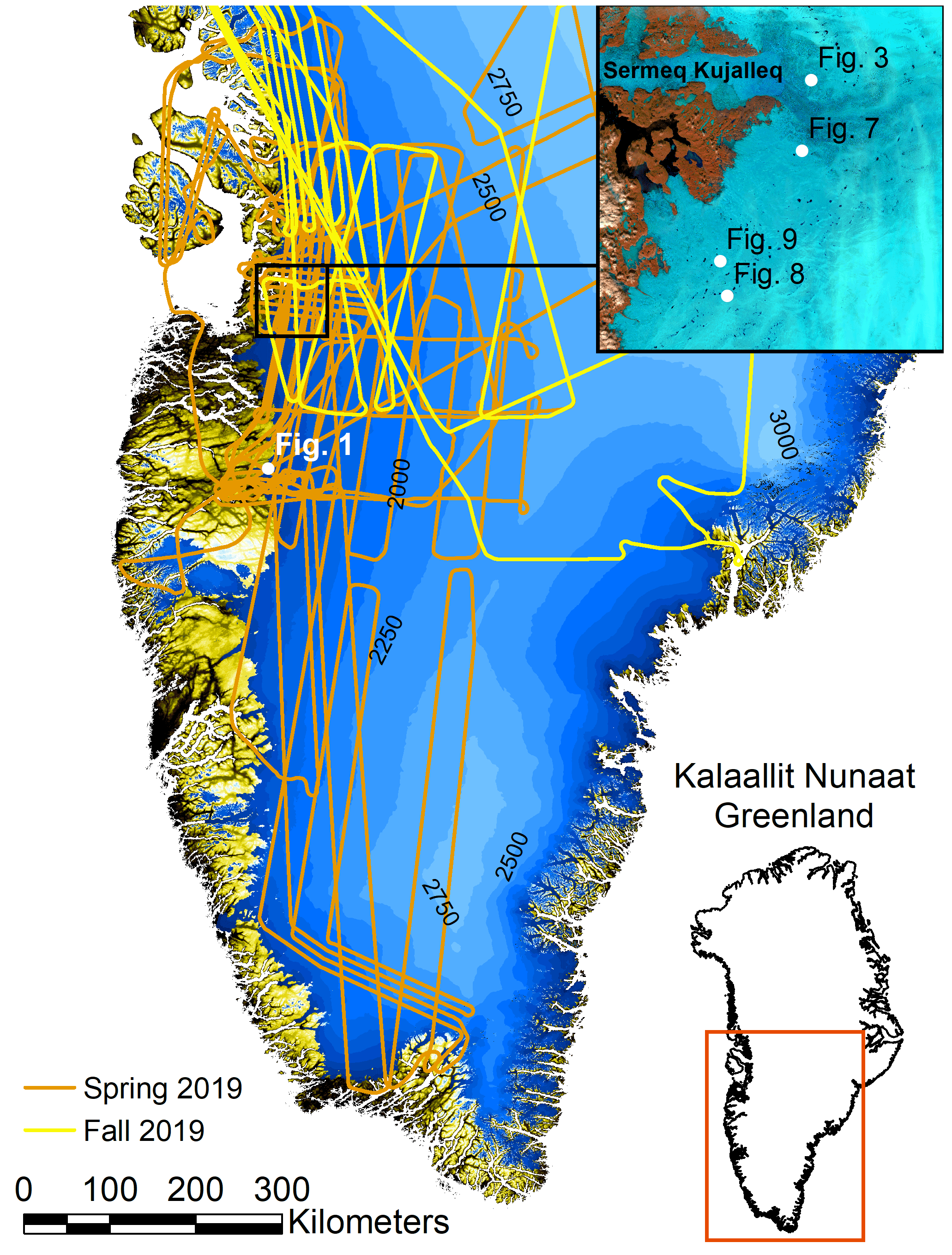
Figure 2Location map with spring and fall 2019 flight lines. Ice surface elevation is shown in blue with a 250 m elevation contour interval. Topography and ice mask data are from the Greenland Ice Mapping Project (GIMP) digital elevation model (Howat et al., 2014; Morlighem, 2021). Inset map over the Sermeq Kujalleq (Jakobshavn Isbræ) region showing figure locations is a Sentinel-2A false color image (bands 11, 8A, and 4) from 17 May 2019.
2.1 Airborne Topographic Mapper (ATM) laser altimeters
The ATM instrument suite contains two conically scanning laser altimeters (lidars) that independently measure the surface elevation along the path of the aircraft at 15∘ and 2.5∘ off-nadir angles (Krabill et al., 2002; MacGregor et al., 2021; Studinger et al., 2020). At a nominal flight elevation of 460 m above ground level (a.g.l.), the swath widths on the ground are 245 and 40 m (MacGregor et al., 2021). The 15∘ wide scanner (ATM T6) transmits at 532 nm wavelength, and the 2.5∘ narrow scanner (T7) transmits at 532 and 1064 nm with co-located green and infrared footprints. Both lasers have a pulse repetition frequency of 10 kHz with a 1.3 ns pulse width (MacGregor et al., 2021; Studinger, 2018). The diameter of the laser footprint on the surface is ∼ 64 cm at 460 m a.g.l.
We use both the Level 1B geolocated point cloud spot elevation measurements for faster detection of supraglacial hydrological features and the much larger Level 1B waveform data product for bathymetry estimates. Table 1 provides a summary of the data sets used.
2.2 ATM natural color imagery
ATM's Continuous Airborne Mapping by Optical Translator (CAMBOT) instrument is a three-channel, natural color, red, green, and blue (RGB) digital camera with 4896 × 3264 pixels and a 28 mm lens. At a nominal flight elevation of 460 m a.g.l., geolocated and orthorectified images span 430 m across track and 290 m along track with a pixel resolution of 7 × 7 cm (MacGregor et al., 2021; Studinger and Harbeck, 2019).
We use both CAMBOT Level 0 raw data (Studinger and Harbeck, 2020) for faster detection of supraglacial hydrological features and the much larger Level 1B geolocated and orthorectified CAMBOT version 2 data product (Studinger and Harbeck, 2019) for analysis of the lidar data. Raw images are collected at 2 Hz, and geolocated data products are provided at 1 Hz, giving sufficient overlap between images at the nominal ground speed of 140 m s−1 for ATM surveys (MacGregor et al., 2021; Studinger and Harbeck, 2019). The footprint-based surface classification described in the next section requires the CAMBOT L1B Version 2 imagery. The geolocated and orthorectified images from the Digital Mapping System (https://nsidc.org/data/iodms1b, last access: March 2022), which are available before the CAMBOT Version 2 imagery was added, do not have the required spatial accuracy over ice sheets for reliable footprint-based surface classification.
A flow diagram summarizing both the image-based processing steps discussed in this section and the process of deriving geolocated water depth estimates, discussed in Sect. 4, is provided in Fig. B3 in the Appendix. We use the normalized difference water index modified for ice (NDWIice) from Yang and Smith (2013) that increases spectral contrast between liquid water and snow and ice surfaces. The NDWIice is defined as
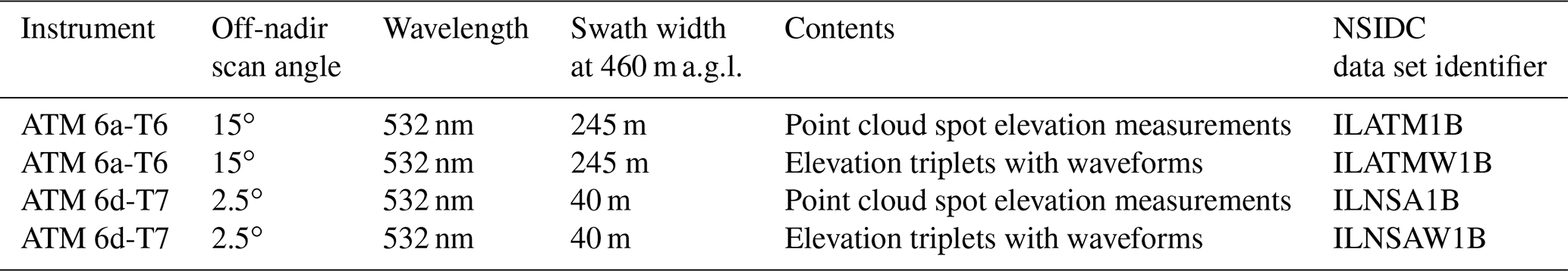
We calculate the NDWIice from CAMBOT RGB images using the blue and red channels. If 10 % of the pixels within a CAMBOT frame exceed an NDWIice threshold of 0.05, we mark that frame as containing a hydrological feature for analysis (Fig. 3).
CAMBOT images are not radiometrically calibrated. CAMBOT is a passive instrument that uses sunlight as the source of illumination. During flight, the camera operator adjusts shutter speed, aperture, and the camera's sensitivity to light (ISO number) to minimize motion blur and optimize exposure over the dynamic range of the camera sensor. The NDWIice threshold used in this paper is an empirical parameter similar to the 10 % threshold of pixels within a CAMBOT frame exceeding the 0.05 NDWIice threshold. Both parameters were determined to be suitable for the spring 2019 campaign and are not absolute thresholds but appear to be stable estimates for the duration of the campaign and the purpose of this paper. It is likely that different campaigns with different light conditions will require adjustment of these thresholds.
We use a Sentinel-2 image mosaic from MacGregor et al. (2020) from August 2019 to delineate the maximum melt and lake extent in 2019 by visual inspection (Fig. 6). We form a spatial mask using this extent to bound the search for hydrological features in the airborne data from May 2019. Whereas meltwater also forms upstream in the catchment areas above the equilibrium line, it primarily pools in lakes and streams below the equilibrium line. We use the approximate elevation of the equilibrium line in the August 2019 Sentinel-2 mosaic as a conservative cut-off elevation mask for identifying hydrological features in airborne data from May 2019. We limit the analysis to CAMBOT images within the melt extent mask and inside the grounded ice mask from Howat et al. (2014) to speed up the feature detection.
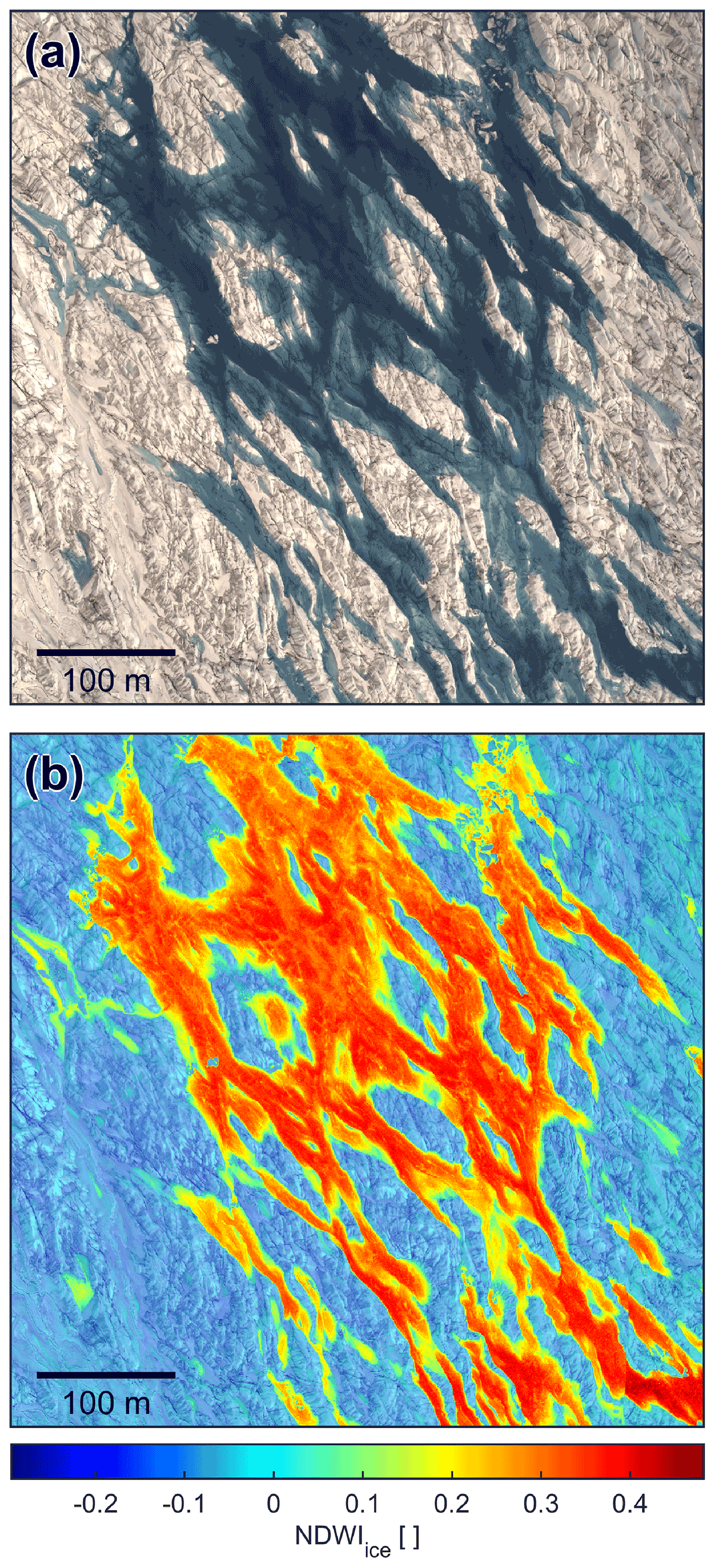
Figure 3(a) Mosaic of three geolocated, orthorectified CAMBOT natural color images of water-filled crevasses on Sermeq Kujalleq (Jakobshavn Isbræ) on 15 May 2019. (b) NDWIice plotted over CAMBOT image mosaic with NDWIice pixels below the detection threshold of 0.05 shown at 50 % opacity. For location see Fig. 2.
Using a simple NDWIice threshold can therefore result in false detections. Dark shadows from elevated topography near the ice margin and shadows in deeply incised crevasses and channels can produce NDWIice values above the detection threshold. More sophisticated, multi-sensor algorithms could be developed to exclude false detections by using, for example, information from the lidar receiver. However, a more complex classification algorithm would be more computationally expensive than the NDWIice method. The bathymetry algorithm described next detects surface and subsurface returns in the lidar data and distinguishes accurately between snow and ice surfaces and hydrological features that have a finite water depth. Therefore, false detections based on NDWIice alone can be eliminated during the lidar analysis; however, they require the presence of a well-defined lake surface from surrounding lidar footprints and cannot be performed on an individual footprint basis. The robustness of the hydrological feature identification is suitable for this paper, since the goal is not to perfectly delineate hydrological features but to identify lidar granules for analysis.
The dielectric contrast between the air–water (lake surface) and the water–ice (lake bottom) interfaces causes reflections of laser energy that can be detected as distinct return pulses. The two-way travel time difference between the lake surface and lake bottom can be used to estimate the depth of hydrological features. The ATM tracking algorithm used for the Level 1B data products is optimized to determine consistent and accurate surface elevations. The ATM tracking algorithm uses 15 % of the maximum amplitude above the baseline as a threshold to determine the centroid of a pulse (Fig. 4a). For overlapping lake surface and bottom return pulses the centroid-based tracker returns an averaged slant range between the surface and bottom of the lake (Fig. 4a). To properly track the surface and bottom returns for overlapping pulses, we use dual-peak Gaussian waveform fitting implemented in a nonlinear regression with seven model parameters. We use MATLAB®'s Signal Processing Toolbox to detect local maxima in the waveforms and use these estimates as initial values as input for the nonlinear regression (Appendix B and Fig. 4b).
Figure 4(a) Centroid estimate (tc) of overlapping surface (S) and bottom (B) return pulses. The centroid-based tracker returns an averaged slant range between the surface and bottom of the lake which in this case is close to the bottom return given the larger amplitude of the bottom return. (b) Gaussian fit of two peaks of overlapping surface (S) and bottom (B) return pulses. The slant range in water between the surface and bottom return pulses t1 and t2 is 33 cm.
For hydrological features, there are several cases that need to be considered to estimate water depth. First, it needs to be determined if a laser shot contains a return pulse from both the surface and the bottom. For some cases, the return from the surface is stronger (Fig. 5a), and for other cases the return from the bottom is stronger (Fig. 5b). For very shallow water depths the surface and bottom returns are typically overlapping (Fig. 5c). Our method is capable of accurately resolving surface and bottom returns in overlapping pulses even if the signal amplitudes are very different (Fig. 5c). For some laser shots there is only a single return which could either be from the lake surface or the much brighter lake bottom. Alternatively, a single return pulse could also be an overlapping surface and bottom return that are so close they appear as a single pulse (Fig. 5d). The algorithm also needs to exclude false pulse detections that are instrument artifacts. The pulses in Fig. 5d are caused by characteristics of the photomultiplier detectors and various other system components such as optical delay fibers and are common in waveform data of airborne and spaceborne lasers (Figs. A2 and A3). The occurrence of these pulses from electronic ringing is consistent in both delay time and percentage of maximum amplitude of the main pulse, and therefore they can reliably be excluded.
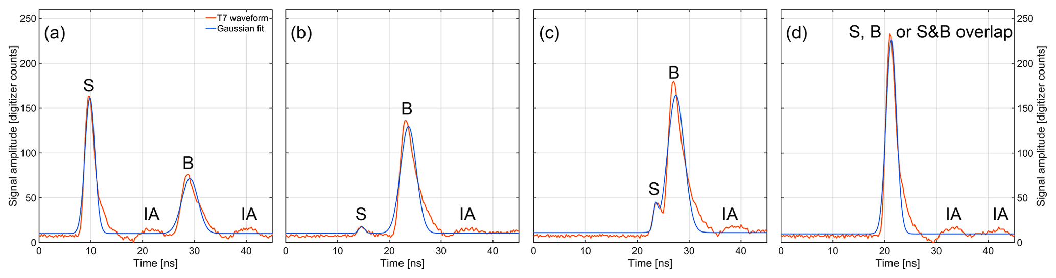
Figure 5Example waveforms of lake return waveforms with Gaussian fits. S marks surface return, B marks bottom return, and IA indicates false return pulses that are caused by instrument artifacts (Fig. A2).
We have evaluated the performance of the nonlinear regression and Gaussian tracker to accurately reproduce the two-way travel time difference as a function of signal-to-noise ratio and pulse separation (Appendix B). A sensitivity analysis of the nonlinear regression was performed by using the mean difference between a prescribed water depth and the depth estimates obtained from linear regression results for 250 000 simulated waveforms with varying signal-to-noise ratios. for each prescribed water depth. Above 0.30 m water depth the difference between the prescribed water depth and the water depth estimated from simulated waveform regressions stabilizes, which we interpret as the reliable detection threshold for the minimum water depth that can be resolved with our approach and instrument system configuration (Fig. B2).
The first step in estimating water depth is to determine the elevation and geolocation of the lake surface return of each laser shot that is consistent with ATM's centroid-based surface elevation tracker used for the Level 1B data products. First, the uncalibrated slant range in air is determined from the two-way travel time difference between the transmit and receive pulse. Then, an intensity-dependent range walk calibration that is determined during the ground test needs to be applied to the uncalibrated ranges to account for the combined effects of delay fibers and other system components on the range estimates. Following that, a range correction needs to be applied to the range estimates due to the atmosphere affecting photon velocity. Scan azimuth and range bias corrections need to be applied as well. All required corrections are provided in the ATM waveform products. The ATM processing flow is detailed in Appendix B and documented in the MATLAB® code published with this paper (https://doi.org/10.5281/zenodo.6341230, Studinger, 2022). The purpose of the approach presented here is not to produce absolute elevation measurements that are accurate and consistent within a campaign and between campaigns but to reliably determine the water depth of supraglacial hydrological features.
Once the elevation and geolocation of the lake surface return have been determined the slant range in water and geolocation of the lake bottom returns are estimated while accounting for the refractive index of water in both geolocation and range. This is done by using Snell's law in vector form in geographic coordinates on the reference ellipsoid. The angle of incidence and geodetic azimuth of the lidar footprint on the lake surface, together with the lake surface elevation, the slant range in water, and the refractive index in air and water, determine the location and elevation of the lidar footprint on the lake bottom.
For laser shots that only have a lake bottom return (e.g., Fig. 5d) the propagation in water needs to be properly accounted for. We first fit a plane through surrounding lake surface elevations and use the resulting elevation of the plane as mean lake surface elevation. We then calculate the intersection of the laser beam transmitted from the aircraft with the mean lake surface using the geodetic azimuth of the laser beam transmitted from the aircraft to the surface target, the off-nadir pointing angle, and the location and elevation of the center of the scan mirror front surface (Fig. A3), which is the fiducial reference point for all two-way travel time estimates. Based on the location of the intersection the slant range and hypothetical two-way travel time between the laser sensor and the intersection of the laser beam with the lake surface can be calculated. Using the hypothetical lidar footprint on the lake surface, the proper location and elevation footprints of laser shots with only lake bottom returns can be calculated.
In general, for waveforms with a lake surface and lake bottom return pulse, the uncertainty of the water depth estimate is primarily a function of the uncertainty of the range estimate of the Gaussian tracker used. We use the data from the T6 and T7 ground tests for this campaign (available at https://doi.org/10.5281/zenodo.6248437, Studinger et al., 2022) to estimate the uncertainty of the Gaussian range estimate to a target with a known distance. The standard deviation of the difference in air between the Gaussian range estimate and the true range to the target is ±0.7 cm when averaged over the entire range of weak pulses just above the detection threshold and heavily saturated pulses. The total uncertainty of the relative range estimate between the surface and the bottom return is the square root of the sum of the squares of the uncertainties of the two range estimates being subtracted and is ±1 cm. For water depth estimates that only have a lake bottom return, additional uncertainty is added that directly scales with the height of the capillary waves on the lake surface.
The primary purpose of this paper is algorithm and method development, and therefore we discuss the bathymetry of only a few select hydrological features here. We have, however, applied the hydrological feature detection algorithm to the entire spring 2019 data set in order to select those examples and begin with a discussion of the example selection and selection criteria.
5.1 Locations of supraglacial hydrological features identified in spring 2019 data: results and discussion
We analyze all CAMBOT Level 0 images from flights between 5 and 16 May 2019 that are below the approximate elevation cutoff for the equilibrium line and within the ice mask. The locations of images with NDWIice exceeding the detection threshold are shown with blue circles in Fig. 6 for central west Greenland. As can be expected, early in the melt season most of the hydrological features are located near the ice margin and at low elevations. We found no compelling evidence for liquid water along our flight lines in southern Greenland in the spring 2019 data. A possible explanation for this is that the ice margin and location of our flight lines are at higher elevations in southern Greenland than they are in central west Greenland and therefore likely exposed to cooler temperatures (Fig. 2). This observation is consistent with the lakes farthest inland being observed in the Sermeq Kujalleq (Jakobshavn Isbræ) area near Ilulissat (Fig. 6) where the ice surface within the Sermeq Kujalleq drainage basin is at lower elevations (Fig. 2) and likely has experienced warmer air temperatures and therefore more melt days than the higher elevations farther south.
We have visually analyzed the images identified as having water surfaces and selected several features that we consider suitable for algorithm and method development. These include a variety of features such as lakes and streams, as well as varying conditions with thin lake ice and surface waves. Lidar data spatial coverage and the depth of lakes are additional criteria used for selection of the below examples. The next section will discuss water depth estimates of these select features.
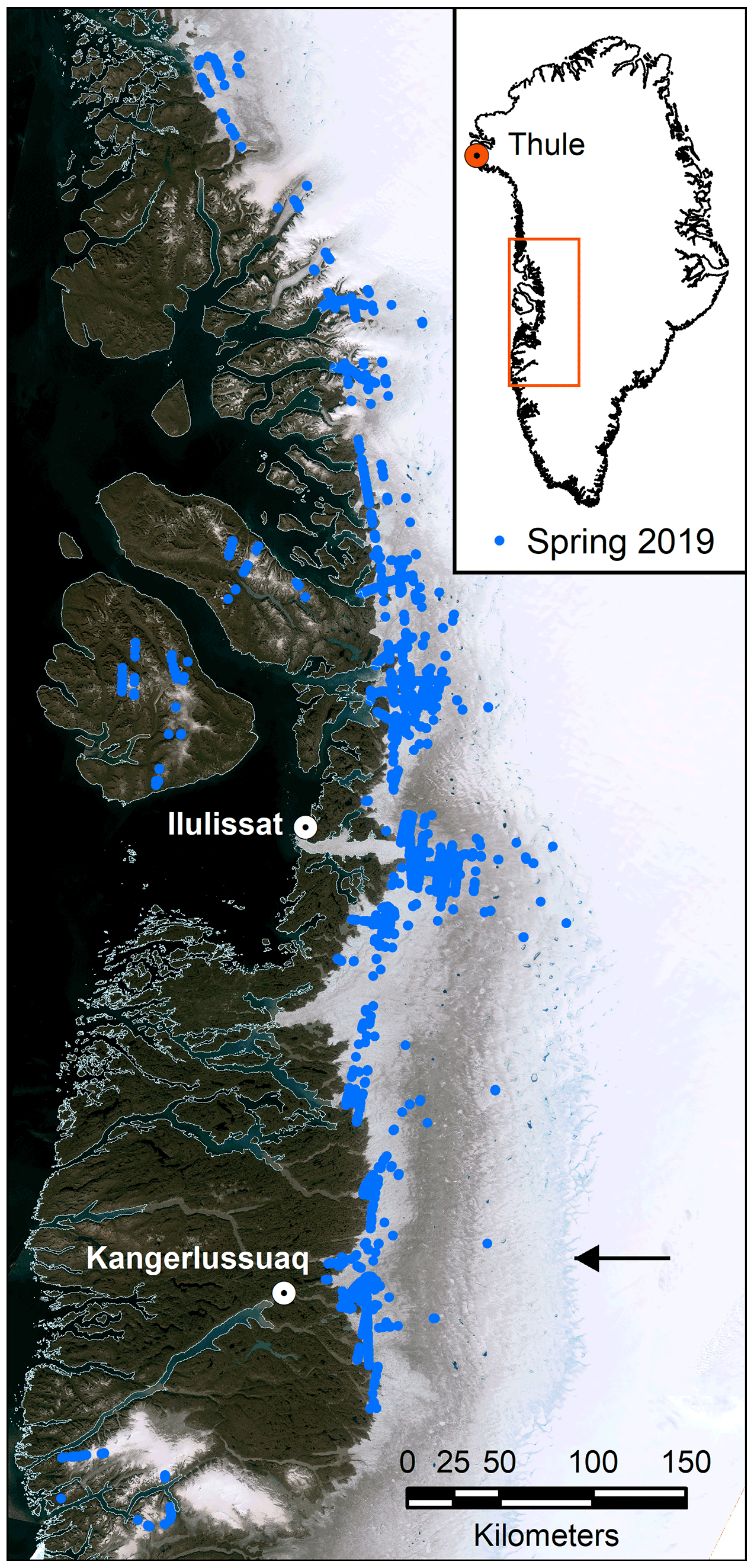
Figure 6Locations of hydrological features in central west Greenland identified in spring 2019 data (blue circles). Background image is a Sentinel-2 image mosaic from MacGregor et al. (2020) from August 2019. The approximate location of the transition between the ablation zone and the accumulation zone (equilibrium line) in August 2019 is indicated by the black arrow.
5.2 Depth estimates of supraglacial hydrological features: results and discussion
The first example, one of the deepest lakes we found, is approximately 140 m wide and 500 m long with complete lidar coverage and a smaller 140 × 40 m lake to the east with partial lidar coverage (Fig. 7). Prior to ATM data acquisition on 6 May 2019 the lake location itself had experienced 6 d of melt since the first recorded onset of melt on 13 April 2019 and 8 d of freezing since then (Fig. A1b). Meltwater that pools in both lakes also forms upstream, but the extent of the catchment area is not known due to a lack of data upstream of the lidar swath. Figure 7a and b illustrate the much denser sampling and level of detail that can be derived from airborne measurements compared to spaceborne measurements. The ICESat-2 data closest in time and space over this lake was acquired on 13 June 2019, 38 d after the ATM pass. Inset map (A) in Fig. 7a shows clearly visible wind-induced waves on the surface of the lake, suggesting that the assumption of a lake surface without waves required for optical depth-based estimates might not be the case for many lakes (Sneed and Hamilton, 2011). Inset map (B) in Fig. 7a shows shadows at the lake bottom from an ice floe at the surface. The length of the shadows could be used together with the elevation and azimuth of the sun at the time of data acquisition to independently estimate the water depth at the edge of the shadow. However, we believe that lidar-based methods are more accurate, in particular since the freeboard of the ice floe is not known without lidar data.
The return signal strength (Fig. 7b) over the lakes and ponds is much weaker than over the snow and ice surfaces seen in the natural-color image mosaic (Fig. 7a) as expected. The return signal strength in Fig. 7b is from the Level 1B point cloud data products (ILATM1B and ILNSA1B, Table 1) and includes lake bottom returns. Furthermore, the wide and narrow scanners are entirely independent lidars, and therefore the absolute return signal strength differs as a result of instrument characteristics and instrument settings during data acquisition. Nevertheless, the correlation between water surfaces visible in the natural-color imagery and relative return signal strength of the lidar data is pronounced. The lower return signal strength also correlates well with NDWIice calculated from natural-color CAMBOT images (Fig. 7b, c). This correlation is also the case for very small ponds marked by circles in Fig. 7b and c. The NDWIice representation (Fig. 7c) reveals narrow meltwater channels connecting the lakes that are difficult to observe in both the natural color and return signal strength data (Fig. 7a, b). The mean lake surface elevation of the small lake east of the main lake is 30 cm above the lake surface of the main lake, implying water from the small lake is flowing downhill into the main lake through the two channels visible in NDWIice data marked by arrows (Fig. 7c).
We use the NDWIice threshold algorithm described in Sect. 3 to assign a surface type (snow and ice, or water) to each lidar footprint for further processing (Fig. 7d). Figure 7e shows the lidar footprint elevations that have been identified as being over either snow and ice or a water surface. The surface returns over the lake show gaps in the northwestern part of the main lake. The gaps are related to the angle of incidence: a combination of the aircraft's pitch and roll angle over the lake segment resulted in a difference in angle of incidence of 9∘ between the northwestern and southeastern parts of the main lake with the southeastern lidar footprints closer to nadir and therefore more likely to trigger recording of a lake surface return. In addition to the aircraft's pitch and roll angle, the geometry of a nutating mirror also results in differences of angles of incidence between forward and aft scan of around 2∘ with the aft scan being closer to nadir. With a flight direction from north to south, Fig. 7e shows that surface returns on the T6 wide scanner are mostly from aft scans as can be expected. The narrow scanner with a 2.5∘ off-nadir scan angle shows almost complete lake surface return coverage.
Figure 7f shows the water depth of the main lake, the small lake to the east, and some of the smaller supraglacial hydrological features such as ponds and channels. Over the main lake, water depths gradually deepen from the shore towards the interior of the lake and reach the maximum depth of 7 m in narrow bottom crevasses (marked by arrows). The ability to resolve these crevasses through water depth measurements illustrates the level of detail that can be derived from airborne measurements. The gradual deepening from the shore to 7 m over the distance of approximately 70 m suggests that the assumption of a homogenous lake bottom that is roughly parallel to the lake surface used for optical depth-based estimates must be used with caution (Sneed and Hamilton, 2011).
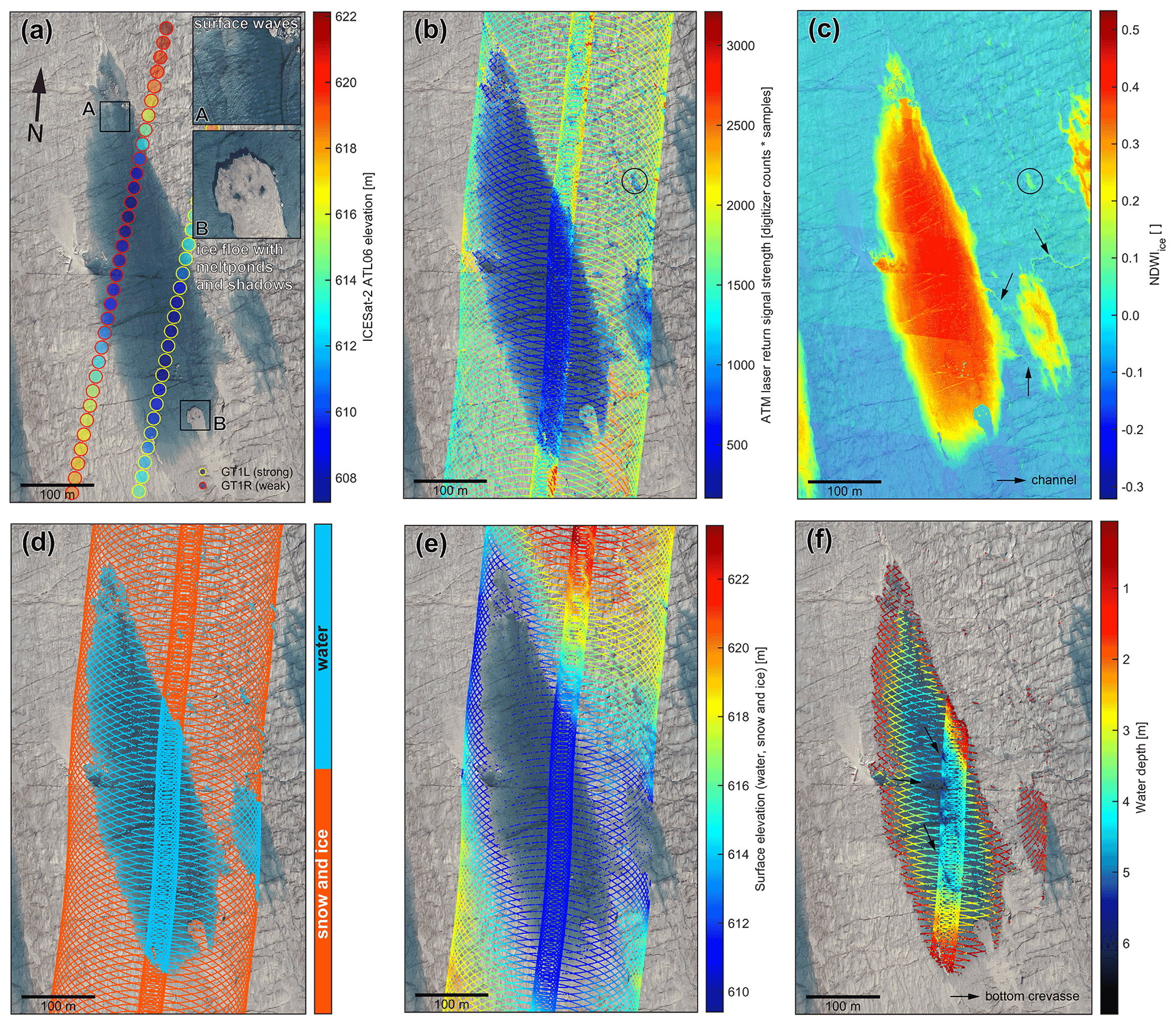
Figure 7(a) Mosaic of five geolocated, orthorectified CAMBOT natural color (red, green, blue) images of a supraglacial lake. ICESat-2 data (Smith et al., 2021) closest in time and space were acquired on 13 June 2019, 38 d after the ATM pass over the lake on 6 May 2019. (b) Return signal strength of the ATM T6 (wide scan) and T7 (narrow scan) laser footprints. The return signal strength is significantly lower over the lake compared to the surrounding snow and ice surface. (c) NDWIice plotted over CAMBOT image mosaic with NDWIice pixels below the detection threshold of 0.05 shown at 50 % opacity. (d) Surface classification of ATM laser footprints based on NDWIice pixels using a classification threshold of 0.05. (e) Surface elevation of laser footprints over snow, ice, and water. (f) Water depth of hydrological features. For location see Fig. 2. Surface temperature and surface melt indicator from MODIS (Hall et al., 2018; Hall and DiGirolamo, 2019) and the number of melt days for this location are shown in Fig. A1b.
The deeper water depths toward the interior of the main lake correlate with higher NDWIice values (Fig. 7c, f). This change in spectral properties with water depth is used in optical depth-based estimates to derive water depths.
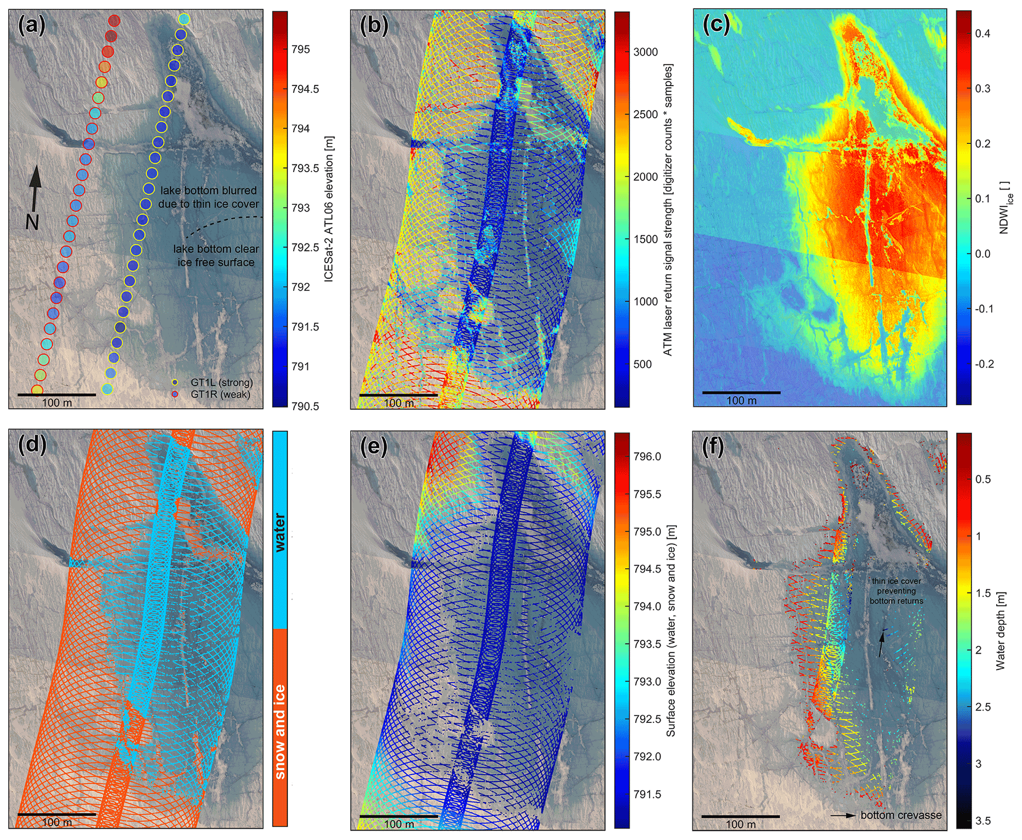
Figure 8(a) Mosaic of five geolocated, orthorectified CAMBOT natural color images of a supraglacial lake. ICESat-2 data were acquired 3 h after the ATM pass over the lake on 15 May 2019. (b) Return signal strength of the ATM T6 and T7 laser footprints. The return signal strength is significantly lower over the lake compared to the surrounding snow and ice surface. (c) NDWIice plotted over CAMBOT image mosaic with NDWIice pixels below the detection threshold of 0.05 shown at 50 % opacity. (d) Surface classification of ATM laser footprints based on NDWIice pixels using a classification threshold of 0.05. (e) Surface elevation of laser footprints over snow and ice. (f) Water depth of hydrological features. For location see Fig. 2. Surface temperature and surface melt indicator from MODIS (Hall et al., 2018; Hall and DiGirolamo, 2019), as well as number of melt days for this location, are shown in Fig. A1c.
The second example (Fig. 8) is a lake with slightly different conditions than the first one. Between the day of the airborne survey on 15 May 2019 and the first reported occurrence of melt on 29 April 2019, this location had experienced 11 d with melt and 6 d without melt (Fig. A1c). The airborne survey was a coordinated ICESat-2 under flight with airborne data acquired just 3 h before ICESat-2 passed over the lake. The lake contains several snow-covered patches of lake ice that are obscuring the view of the lake bottom and prevent enough lidar light to reach the lake bottom necessary to trigger the recording of a bottom return pulse (Fig. 8a). Thin layers of lake ice impose limitations not only for airborne and spaceborne lidar-based water depth estimates but also for any optical depth-based bathymetry estimates. The high-resolution natural color imagery reveals relevant details that currently cannot be identified with spaceborne sensors. On the eastern side of the lake, there is a sharp transition in the visibility of details such as crevasses and other structures on the lake bottom to a blurred lake bottom north of it (Fig. 8a). While not discernible in the natural color imagery, it is likely that the blurring of the lake bottom is caused by a thin layer of clear lake ice. This thin ice cover also acts as a specular reflector for laser light and likely reflects lidar energy away from the detector, thereby causing gaps in bottom returns. This interpretation is supported by the weaker return signal strength over the area with thin ice cover compared to the ice-free water surface south of it (Fig. 8b). Figure 8c shows some of the limitations of using a simple NDWIice detection threshold for surface classification. When exposure time between CAMBOT frames is either automatically or manually adjusted, the brightness of pixels and therefore the NDWIice value of the same feature changes from frame to frame, as can be seen in Fig. 8c. However, the visual correlation with water surfaces in the natural color imagery (Fig. 8a), the lidar return signal strength (Fig. 8b), and the lidar footprint surface classification (Fig. 8d) show that an NDWIice detection threshold is a robust surface classification method for the purpose of this paper.
The water depth within this lake gradually deepens from its western shore towards the interior of the lake before becoming shallower again. The deepest returns are around 3.5 m, but most of the deepest part of the lake lacks bottom returns. As can be seen in Fig. 8e, the loss of bottom returns is not a simple function of water depth alone. Some of the deepest returns are located within a narrow bottom crevasse (marked by an arrow in Fig. 8e) that has no returns in the shallower part around it. A possible explanation for this is that the slope of the sidewalls of the crevasse or channel is closer to the normal of the lidar beam than in the surrounding areas, and therefore lidar light is reflected to the sensor on the aircraft. Also, concave-shaped surfaces, such as those found in crevasses and channels, can have a focusing effect that increases the intensity of the reflected lidar light and increases the likelihood of exceeding the signal strength necessary to trigger recording of a bottom return pulse.
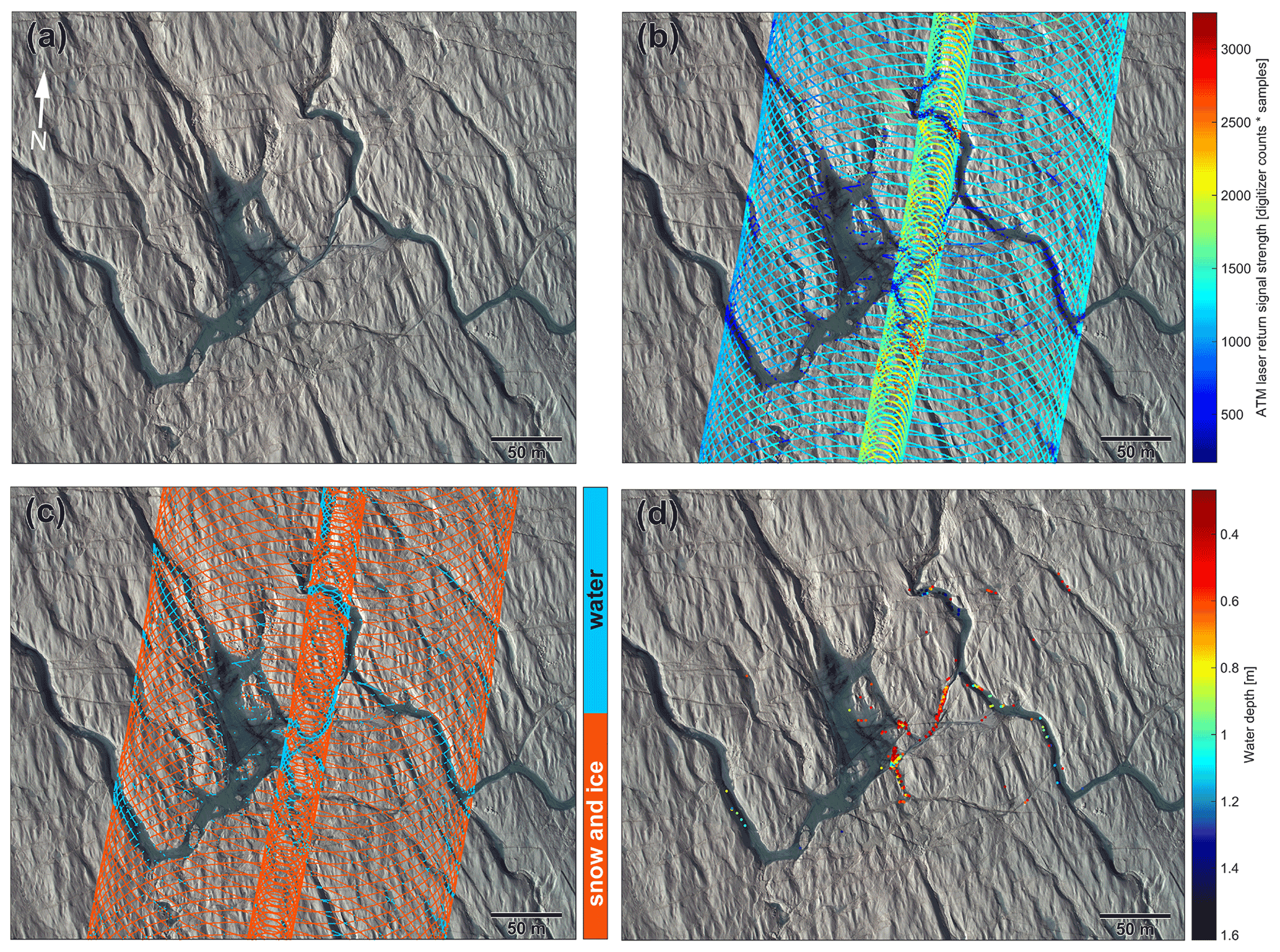
Figure 9(a) Mosaic of two geolocated, orthorectified CAMBOT natural color images of a supraglacial lakes, streams, and channels from 12 May 2019. (b) Return signal strength of the ATM T6 and T7 laser footprints. (c) Surface classification of ATM laser footprints based on NDWIice pixels using a classification threshold of 0.05. (d) Water depth of hydrological features. For location see Fig. 2. Surface temperature and surface melt indicator from MODIS (Hall et al., 2018; Hall and DiGirolamo, 2019), as well as number of melt days for this location, are shown in Fig. A1d.
The third example shows a network of narrow, 5–10 m wide meltwater channels and streams and reflects the most challenging targets for bathymetric imaging found in this study (Fig. 9). Following the first reported melt between 29 April 2019 and the day of the airborne survey, this location had experienced 11 d of melt and 1 d of freezing (Fig. A1d). There are no ICESat-2 footprints within the extent of the data frame shown. In general, we find that channels and streams show a very low number of both surface and bottom returns compared to lakes (Fig. 9). A possible explanation is that these narrow streams flow in topographic channels that provide more protection from surface winds compared to relatively open lakes shown in Figs. 7 and 8. Wind protection hinders generation of surface capillary waves, which are necessary to reflect lidar energy back to the sensor on the aircraft. The presumably flat water surface of these streams acts as a specular reflector directing lidar energy away from the sensor and resulting in very few surface and bottom returns. The deepest returns of around 1.6 m can be seen in a bend of a channel near the northern end of the data frame.
We compared pulse widths of lake surface and lake bottom return pulses of the hydrological features we have discussed, and we found no relationship between pulse width and slant range in water potentially caused by volume scattering in water. In addition to volume scattering in water the slope and roughness of the lake bottom will likely be bigger contributors to pulse widening than volume scattering. The extremely clear water visible in true-color imagery suggests very low turbidity of these water bodies, which in turn should result in very little volume scattering and associated pulse broadening.
ATM's suite of co-located sensors, small laser footprints (64 cm), high shot density, swath coverage, and high-resolution imagery (10 cm) reveals fine-scale hydrological features, such as very narrow meltwater channels and surface waves, that cannot be detected from space. Airborne measurements can also image supraglacial hydrological features at a spatial scale and coverage that cannot be achieved by local measurements from short-range drones, which are often operated out of remote field camps and require line-of-sight communications. The accuracy and resolution from airborne measurements compared to spaceborne sensors provides critical complementary information that can support calibration and validation of spaceborne methods and provide information necessary for high-resolution process studies of the supraglacial hydrological system on the GrIS that currently cannot be achieved from spaceborne observations alone. The minimum water depth that can be resolved with the current algorithm using a 1.3 ns laser pulse sampled at 4 GHz is around 30 cm, and the maximum water depth measured with the ATM optimized for snow and ice elevation measurement was around 7 m. However, this could also reflect the maximum water depth encountered early in the melt season rather than an instrument limitation.
ATM KT19 infrared surface temperatures
The KT19 is an infrared radiation pyrometer that is used to measure infrared radiation wavelengths between 960 and 1150 nm that are used to derive skin temperatures within the field of view of the sensor. At a nominal flight elevation of 460 m a.g.l., the 2∘ field of view of the sensor results in an approximately 15 m measurement footprint on the surface. Measurements are taken at 10 Hz (Studinger, 2019).

Figure A1Surface temperature (black crosses) and surface melt indicator (red and blue circles) from MODIS (Hall et al., 2018; Hall and DiGirolamo, 2019) and mean ATM KT19 infrared surface temperatures (Studinger, 2019) averaged in 60 s windows over the hydrological features with 1σ standard deviation. The windows of operation of the spring and fall 2019 campaigns are indicated by vertical gray areas in all panels. Panel (a) show the times series for the approximate location of the oblique aerial photograph in Fig. 1, panel (b) is for the lake shown in Fig. 7, panel (c) is for the location of the lake shown in Fig. 8, and panel (d) is for the location of the streams and channels shown in Fig. 9.
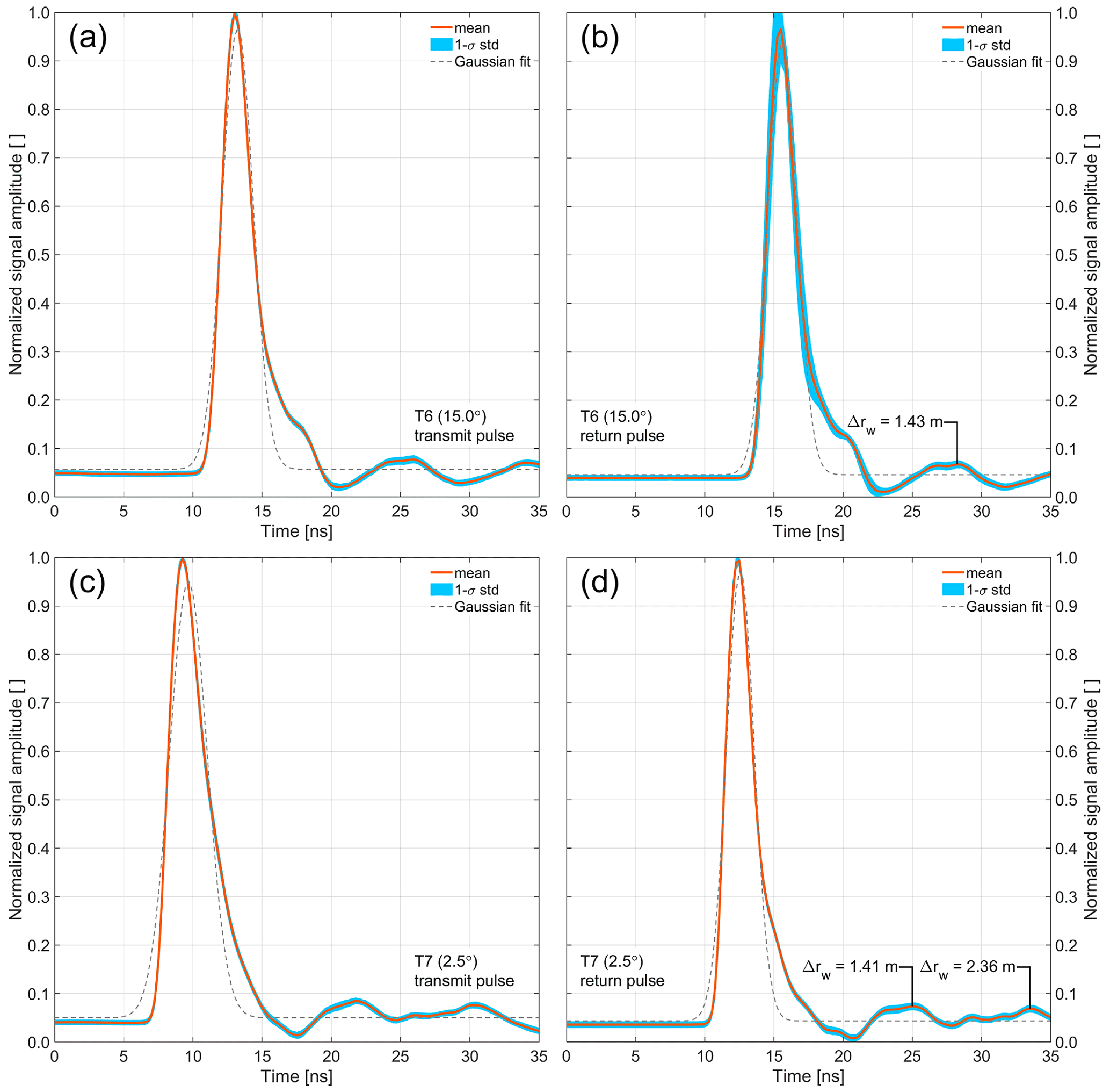
Figure A2Averaged, normalized, unsaturated transmit and return waveforms of the T6 (a, b) and T7 (c, d) transceivers acquired over the airport ramp in Kangerlussuaq, Greenland, on 13 May 2019. The impact of surface slope and surface roughness of the ramp's concrete surface within an ATM laser footprint does not contribute to the shape of the return waveform and can be neglected. The concrete surface has no subsurface penetration for 532 nm laser light. The main peak is followed by smaller artifact peaks, the first of which occurs 12.75 ns after the main peak in T6 and 12.5 ns in the T7 waveforms. The difference between T6 and T7 corresponds to one sample for a digitization rate of 4 GHz (0.25 ns). The second peak in T7 occurs 21 ns after the surface return. The corresponding slant range in water is Δrw. All three peaks have an amplitude of 7 % of the surface return. A total of 28 084 waveforms were stacked for T6, and 48 703 waveforms were stacked for T7. The deviation from a Gaussian shape is the combined result of characteristics of the laser, photomultiplier detectors, and various other system components such as optical delay fibers and are common in waveform data of airborne and spaceborne lidars (Fig. A3).
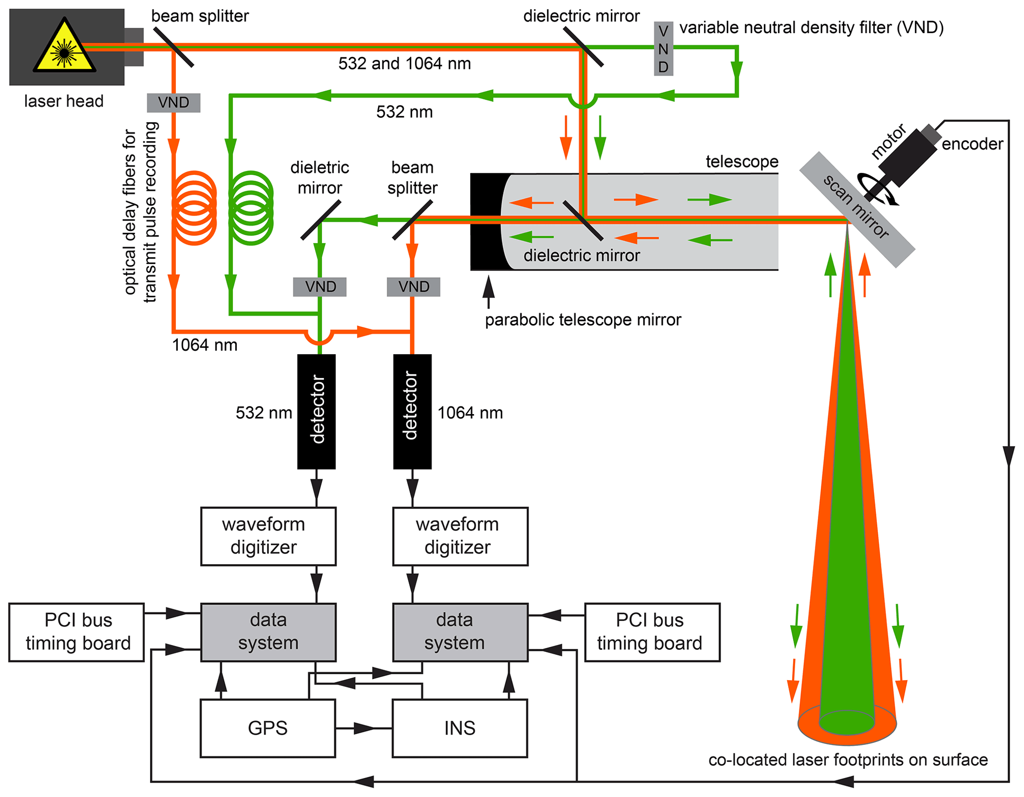
Figure A3Schematic diagram of ATM's dual color T7 transceiver with co-located green (532 nm) and IR (1064 nm) footprints.
This section describes the processing flow for the ATM lidar data used in this paper for estimating surface elevations and water depths. The MATLAB® code is available at https://doi.org/10.5281/zenodo.6341230 (Studinger, 2022).
B1 Geolocation of the laser sensor
The position of the Global Navigation Satellite System (GNSS) antenna on top of the fuselage of the survey aircraft is determined from NAVSTAR Global Positioning System (GPS) and Globalnaya Navigatsionnaya Sputnikovaya Sistema (GLONASS) carrier phase measurements recorded by receivers on the aircraft. These measurements are combined in post-flight processing with similar measurements from multiple static ground stations to determine a kinematic differential solution (DGPS) of the antenna trajectory. The lever arm from antenna to ATM scan mirror provided in the ATM waveform data products includes corrections for aircraft-specific changes in antenna phase centers that are determined for each campaign. The reference point for all lidar measurements is the scan mirror fiducial point (Fig. A3). To determine the location of the scan mirror fiducial point in both space and time, the DGPS solutions are combined with aircraft attitude measurements from a commercial inertial navigation system (INS) on the survey aircraft, often also referred to as inertial measurement unit (IMU), and measurements of the lever arm between the antenna and scan mirror in an aircraft-fixed cartesian coordinate system with the origin in the phase center of the antenna. The coordinate translations and rotations are done in a geocentric ECEF (Earth-centered, Earth-fixed) coordinate system, which are then converted to geographic coordinates for the position of the laser sensor.
B2 Determination of time of flight and uncalibrated raw ranges using a centroid-based tracking algorithm
The two-way travel time difference Δt (i.e., the time of flight) is determined using the centroid of the transmit (ttx) and receive (trx) pulses. The centroid tc of a discrete waveform w(t) is defined as
w(t) is the amplitude recorded by the waveform digitizer (in counts) minus the baseline, which is estimated from the median of the first 21 samples of the waveform. The ATM tracking algorithm used for the data presented in this paper uses 15 % of the maximum amplitude above the baseline as a threshold to determine tstart by interpolating between samples. Similarly, tend is defined as the first interpolated point where w(t) falls below the 15 % threshold. The uncalibrated range runcal between the two centroids of the transmit and receive pulse is
where c is the speed of light in vacuum.
B3 Range calibration determined from ground calibration data
In a pressurized aircraft, the transmitted laser pulse travels thru the aircraft's optical window close to the scan mirror (Fig. A2). Backscatter from both the scan mirror and the aircraft's optical window in the fuselage is close in time to the transmitted laser pulse and partially overlap with the transmit waveform. To record a “clean” transmit waveform the transmit pulse is sampled from behind a translucent beam splitter and subsequently injected into a multimode fiber-optic cable to provide a fixed optical delay that results in temporal separation between the recorded transmit pulse and contamination from backscattered photons from the scan mirror and the aircraft's optical window (Fig. A3). The optical delay fiber and other system components introduce a laser time-of-flight range bias that needs to be determined from ground calibration measurements.
In addition to measuring the instrument's system delay the second purpose of
the ground calibration is to determine the intensity-varying change in range
that is known as range walk. ATM data are collected from a stationary target
at known range while varying the return intensity from signal extinction to
detector saturation. The waveform tracking method used will result in
apparent changes in range from the stationary target, and these data can be
applied as a range correction. The ground test calibration values combine
the system delay and range walk correction and are subtracted from the
uncalibrated ranges to yield the calibrated range estimates (/laser/calrng) in
the airborne waveform files. The ground test data and
MATLAB® code used in this paper for reading the
ground test waveform data are available at https://doi.org/10.5281/zenodo.6248437 (Studinger et al.,
2022).
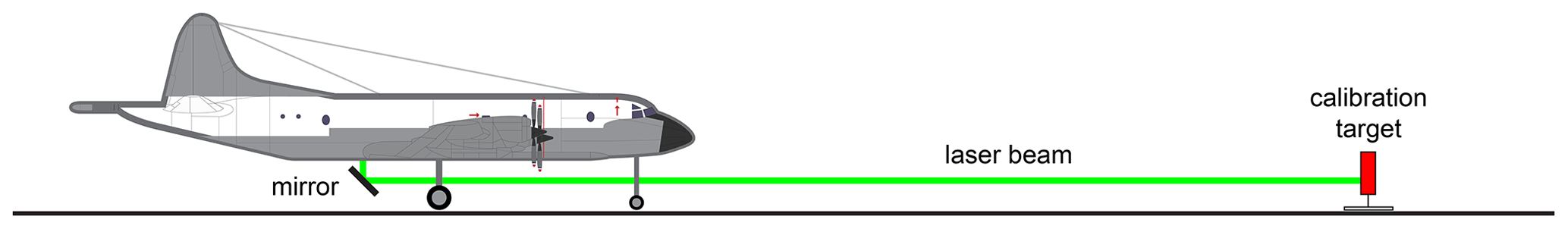
Figure B1Range bias determination (a.k.a. ground test) using a calibration target with a known distance. The range to the calibration target is measured with an electronic distance meter (a.k.a. “total station”) with an accuracy of a few millimeters.
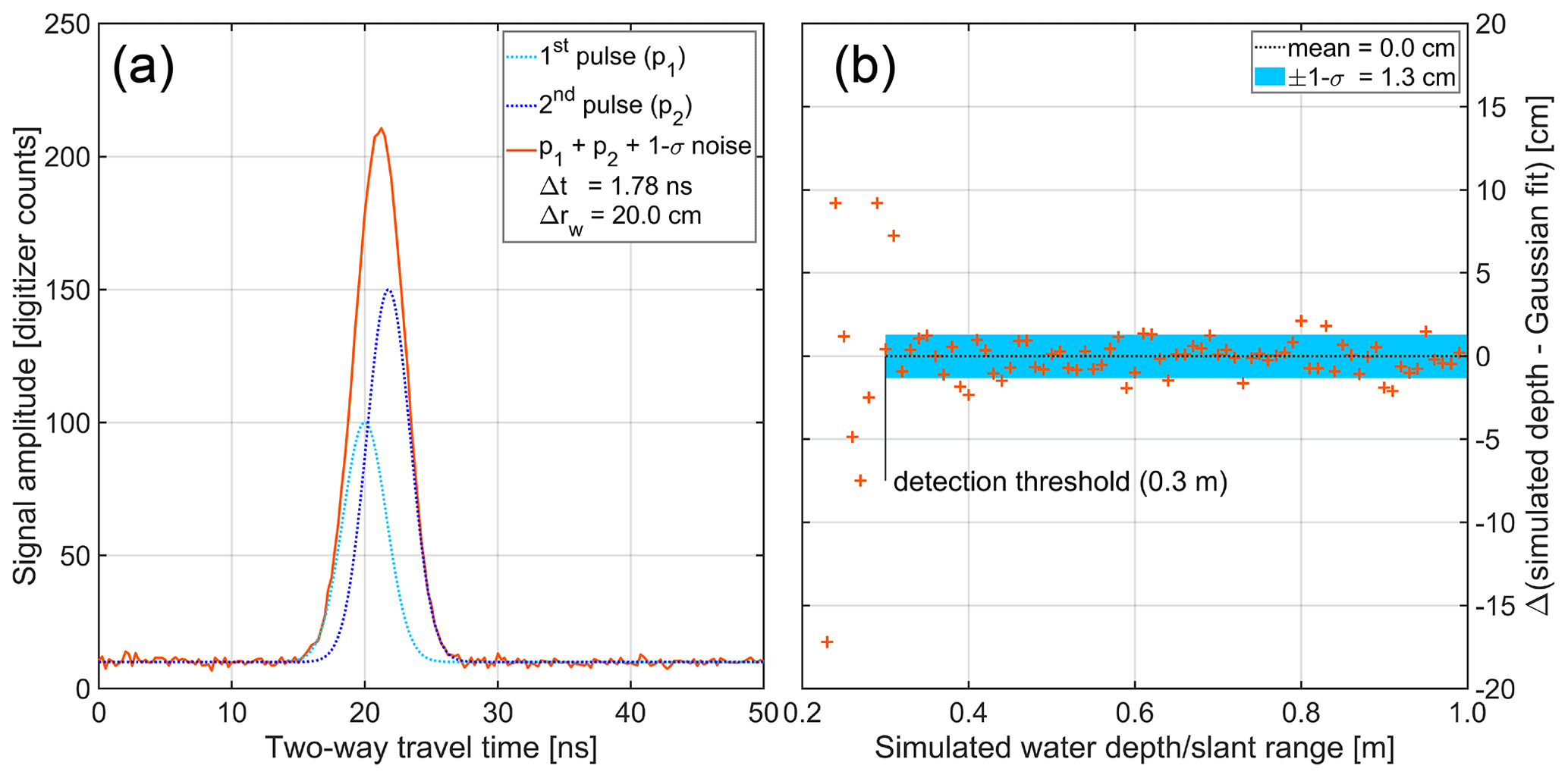
Figure B2(a) Synthetic Gaussian waveforms of overlapping surface and bottom return pulses. The FWHM pulse width is 1.6 ns (1σ), and the mean of the two pulses is separated by Δt=1.78 ns, which corresponds to a slant range Δrw=20 cm in water. The combined waveform has the average ATM T6 and T7 system noise level added. The two pulses are not discernible in the combined waveform. (b) Sensitivity analysis of the nonlinear regression. The mean of difference between the synthetic water depth and the 250 000 nonlinear regressions for each water depth is shown (orange crosses), and the standard deviation (1σ) and mean for water depths greater than the determined detection threshold of 0.30 m are shown.
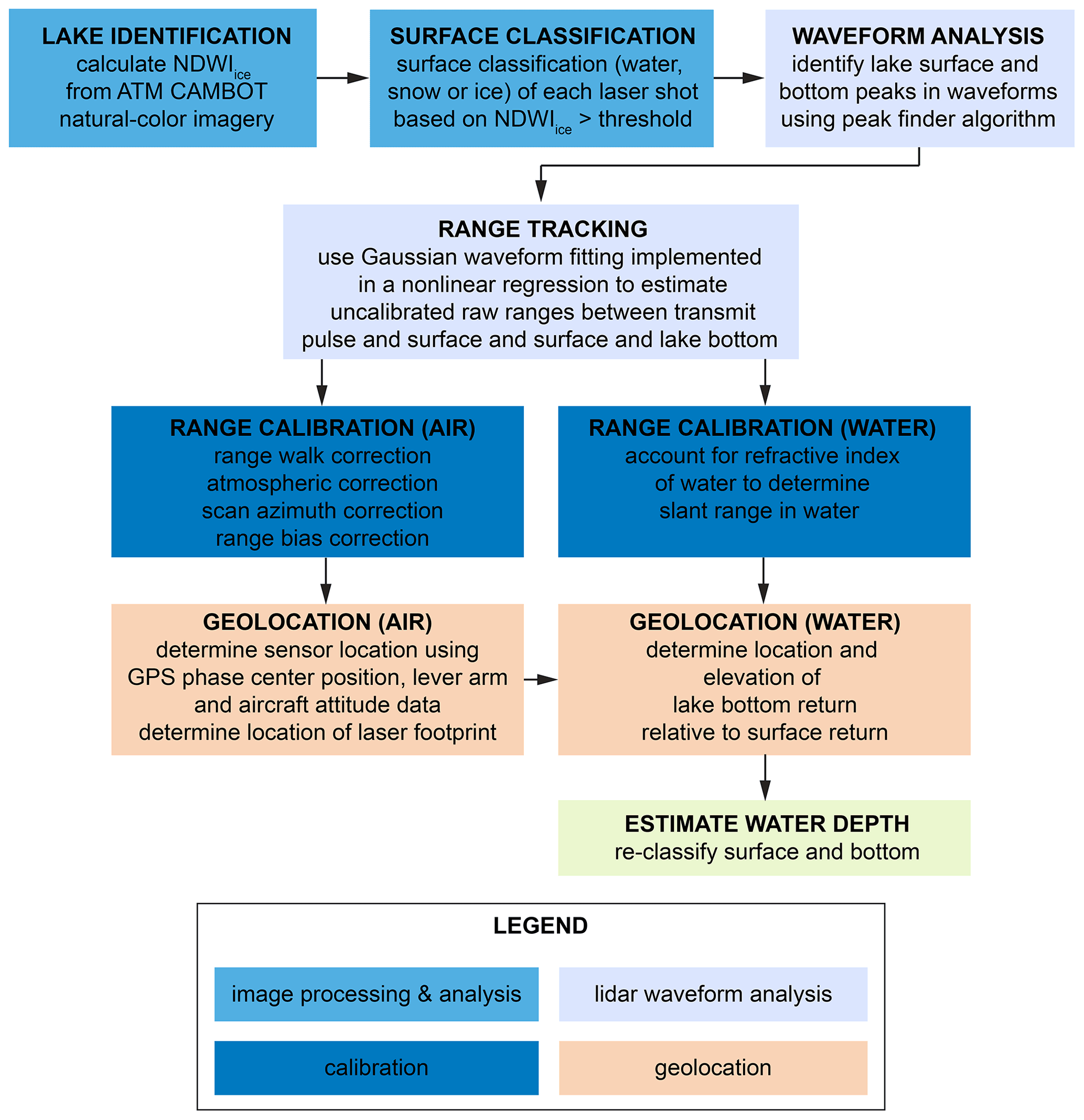
Figure B3Flow diagram summarizing both the image-based processing steps discussed in this section and the process of deriving geolocated water depth estimates from lidar data discussed in Sect. 4.
B4 Determination of mounting biases
Martin et al. (2012) describe the process of estimating the six mounting biases related to range, scan angle, attitude, and position using ramp passes and cross-over analysis. Harpold et al. (2016) describe an alternative approach using the difference between forward and aft scan elevations. These six biases are already applied to the data in the HDF5 waveform files available from NSIDC.
B5 Scan azimuth bias correction
Some campaigns contain scan-azimuth-dependent elevation biases that can
change over the course of a flight or a campaign. The elevation biases are a
function of scan azimuth and are stored in /mounting_parameters/scan_elv_adj. The elevation error
due to azimuth error scales with the aircraft's elevation above ground level. It is determined for the nominal flight elevation (1500 ft or 457 m).
Scaling the correction with elevation is done by multiplying the aircraft's
above ground level with the elevation biases provided in the waveform data and dividing it
by the nominal flight elevation (457 m). The resulting elevation-scaled
values using /mounting_parameters/scan_elv_adj and /aircraft/AGL are subtracted from the elevation
values. The lidar data from the spring 2019 campaign used in this paper did
not require scan azimuth bias corrections.
B6 Atmospheric range correction
The propagation speed of light is lower in a denser medium such as the
atmosphere compared to vacuum. In laser altimetry, this effect is referred
to as atmospheric delay. The density of the atmosphere at the time and
position of the aircraft and the footprint on the surface can be calculated
from parameters provided by global numerical weather models. The density is
primarily a function of the temperature of air, the atmospheric pressure,
and the partial pressure of water vapor and can be used to calculate the
refractive index along the propagation path of a laser beam. The range correction applied due to the atmosphere
affecting photon velocity is provided in /laser/atmos_cor for
each elevation measurement in the HDF5 waveform files and needs to be
applied to the range estimates. The /laser/atmos_cor values
are subtracted from the /laser/calrng slant ranges.
B7 Range bias
The ultimate reference for in-flight data are the ramps, crossings, and
along-track comparisons to produce consistent elevation measurements over
the course of a campaign and between campaigns. Any residual bias thus
determined (typically on the order of a few centimeters) is included in
/mounting_parameters/range_bias, which are
added to the range estimates (not elevation). The /mounting_parameters/range_bias is typically the same for an entire
deployment but can change when there is a hardware change (e.g., fiber
swap, change fiber pickoff location) during a deployment.
B8 Gaussian fit
The lake surface and lake bottom returns are fitted with a dual-peak Gaussian function g2(t) with seven parameters:
where b is the signal baseline (noise floor), a1,2 are the pulse amplitudes, t1,2 are the pulse locations of the pulse maxima and means, and σ1,2 are the 1-sigma (1σ) pulse widths. The nonlinear regression is done using initial values estimated using output from MATLAB®'s Signal Processing Toolbox findpeaks as input for MATLAB®'s Statistics and Machine Learning Toolbox nlinfit function.
B9 Sensitivity analysis
The performance of the nonlinear regression to accurately reproduce the two-way travel time difference is primarily a function of pulse separation. For a 20 cm slant range in water the two-way travel time difference between the surface and bottom return pulses is 1.78 ns (Fig. B2a), which is close to the average pulse width of 1.63 ± 0.71 ns (1σ), or 3.84 ± 1.68 ns (FWHM: full width at half maximum) of the ATM T6 return laser pulse estimated from ground tests using a penetration-free target (Fig. B1). The average return pulse width of T7 has been estimated to be 1.20 ± 0.31 ns (1σ) or 2.82 ± 0.74 ns (FWHM). We also estimated the standard deviation (1σ) of the baseline noise before the arrival of the return pulse from ground tests to be 0.9 ± 0.1 digitizer samples for both T6 and T7. The standard deviation of the electronic noise discernible in the signal baseline is stable over the course of a campaign and does not change. We combine two synthetic Gaussian waveforms simulating the surface and bottom return pulse from a prescribed water depth into a single waveform and add random signal noise with the 1σ standard deviation estimated from the actual lidar data to each waveform for input into our sensitivity analysis. In addition to the baseline noise, we also randomly vary the signal-to-noise level (maximum pulse amplitude above baseline vs. standard deviation of electronic noise) in each simulated waveform with the range possible in the actual lidar data. The minimum amplitude to trigger signal acquisition for the discussed data set is 36 digitizer counts for both T6 and T7 resulting in a possible signal-to-noise ratio range between 29:1 to 248:1 above the baseline for an 8 bit digitizer (7.0 ± 0.2 digitizer counts for T6 and 8.5 ± 0.5 digitizer counts for T7). We have varied the simulated water depths in 0.01 m increments between 0.2 and 1.0 m and created 250 000 simulated waveforms with varying signal-to-noise ratios for each prescribed water depth. We have then estimated the water depth for each waveform and plotted the mean difference between the described water depth and the water depths estimated from each linear regression in Fig. B2b. We have increased the number of regressions for each prescribed water depth until the results were stable and found 250 000 to be a conservative number. There is a noticeable change in the magnitude of scatter of the differences at 0.3 m which we determine to be the minimum depth threshold to be used for our analysis (Fig. B2b).
The MATLAB® code developed for this paper for tracking lake surface and lake bottom returns, analyzing waveforms, geolocating ATM lidar footprints, and calculating water depths is available at https://doi.org/10.5281/zenodo.6341230 (Studinger, 2022).
Chad Greene's MATLAB® function for interpolating GeoTIFF data is available on MATLAB®`s File Exchange website at https://www.mathworks.com/matlabcentral/fileexchange/47899-geotiffinterp (Greene, 2022).
All ATM Operation IceBridge airborne data used in this study are freely available at the National Snow and Ice Data Center at https://nsidc.org/icebridge/portal (last access: March 2022). The ATM waveform data from the two ground tests used here, the true ranges, and MATLAB® code for reading ground test data are available at https://doi.org/10.5281/zenodo.6248437 (Studinger et al., 2022). The ATLAS/ICESat-2 L3A Land Ice Height data (ATL06) are available from NSIDC at https://doi.org/10.5067/ATLAS/ATL06.004 (Smith et al., 2021).
Greenland-wide topography and ice mask data are from the Greenland Ice Mapping Project (GIMP) digital elevation model (Howat et al., 2014; Morlighem, 2021) and are available at NSIDC at https://doi.org/10.5067/VLJ5YXKCNGXO (Morlighem, 2020).
The Sentinel-2 image mosaic from August 2019 from MacGregor et al. (2020) is available through QGreenland at https://qgreenland.org/ (last access: March 2022) or https://doi.org/10.5281/zenodo.5548326 (Moon et al., 2021).
The ice surface temperature and ice surface melt indicator from MODIS (Hall et al., 2018; Hall and DiGirolamo, 2019) are available at NSIDC at https://doi.org/10.5067/7THUWT9NMPDK (Hall and DiGirolamo, 2019).
The Sentinel-2A image used in Fig. 2 is available from the USGS EarthExplorer website at https://doi.org/10.5066/F76W992G (European Space Agency, 2022).
MS led the analysis of the laser altimetry, optical imagery, and integration of results and prepared the manuscript. All authors helped interpret the analysis, develop the methods, and comment on the manuscript.
The contact author has declared that none of the authors has any competing interests.
Publisher’s note: Copernicus Publications remains neutral with regard to jurisdictional claims in published maps and institutional affiliations.
This paper reflects the combined efforts of all ATM team members over many decades of instrument development and field deployments. Jeremy Harbeck and Nathan Kurtz are thanked for developing the ATM CAMBOT L1B Version 2 data product. We thank the Operation IceBridge flight crews that made data collection for this study possible. We thank the editor Louise Sandberg Sørensen and two anonymous reviewers for thoughtful comments that helped improve the manuscript.
This work was funded by NASA’s Internal Scientist Funding Model and the Airborne Science Program.
This paper was edited by Louise Sandberg Sørensen and reviewed by two anonymous referees.
Box, J. E. and Ski, K.: Remote sounding of Greenland supraglacial melt lakes: implications for subglacial hydraulics, J. Glaciol., 53, 257–265, https://doi.org/10.3189/172756507782202883, 2007.
Chu, V. W.: Greenland ice sheet hydrology:A review, Prog. Phys. Geog., 38, 19–54, https://doi.org/10.1177/0309133313507075, 2014.
Corr, D., Leeson, A., McMillan, M., Zhang, C., and Barnes, T.: An inventory of supraglacial lakes and channels across the West Antarctic Ice Sheet, Earth Syst. Sci. Data, 14, 209–228, https://doi.org/10.5194/essd-14-209-2022, 2022.
Das, S. B., Joughin, I., Behn, M. D., Howat, I. M., King, M. A., Lizarralde, D., and Bhatia, M. P.: Fracture Propagation to the Base of the Greenland Ice Sheet During Supraglacial Lake Drainage, Science, 320, 778–781, https://doi.org/10.1126/science.1153360, 2008.
Datta, R. T. and Wouters, B.: Supraglacial lake bathymetry automatically derived from ICESat-2 constraining lake depth estimates from multi-source satellite imagery, The Cryosphere, 15, 5115–5132, https://doi.org/10.5194/tc-15-5115-2021, 2021.
Enderlin, E. M., Howat, I. M., Jeong, S., Noh, M.-J., van Angelen, J. H., and van den Broeke, M. R.: An improved mass budget for the Greenland ice sheet, Geophys. Res. Lett., 41, 866–872, https://doi.org/10.1002/2013gl059010, 2014.
European Space Agency: USGS EROS Archive – Sentinel-2, USGS Earth Resources Observation and Science Center [data set], https://doi.org/10.5066/F76W992G, 2022.
Fair, Z., Flanner, M., Brunt, K. M., Fricker, H. A., and Gardner, A.: Using ICESat-2 and Operation IceBridge altimetry for supraglacial lake depth retrievals, The Cryosphere, 14, 4253–4263, https://doi.org/10.5194/tc-14-4253-2020, 2020.
Flowers, G. E.: Hydrology and the future of the Greenland Ice Sheet, Nat. Commun., 9, 2729, https://doi.org/10.1038/s41467-018-05002-0, 2018.
Greene, C: geotiffinterp, MATLAB Central File Exchange [data set], https://www.mathworks.com/matlabcentral/fileexchange/47899-geotiffinterp, 2022.
Hall, D. K. and DiGirolamo, N. E.: Multilayer Greenland Ice Surface Temperature, Surface Albedo, and Water Vapor from MODIS, Version 1 (MODGRNLD), NASA [data set], https://doi.org/10.5067/7THUWT9NMPDK, 2019.
Hall, D. K., Cullather, R. I., DiGirolamo, N. E., Comiso, J. C., Medley, B. C., and Nowicki, S. M.: A Multilayer Surface Temperature, Surface Albedo, and Water Vapor Product of Greenland from MODIS, Remote Sensing, 10, 555, https://doi.org/10.3390/rs10040555, 2018.
Harpold, R., Yungel, J., Linkswiler, M., and Studinger, M.: Intra-scan intersection method for the determination of pointing biases of an airborne altimeter, Int. J. Remote Sens., 37, 648–668, https://doi.org/10.1080/01431161.2015.1137989, 2016.
Howat, I. M., Negrete, A., and Smith, B. E.: The Greenland Ice Mapping Project (GIMP) land classification and surface elevation data sets, The Cryosphere, 8, 1509–1518, https://doi.org/10.5194/tc-8-1509-2014, 2014.
Krabill, W. B., Abdalati, W., Frederick, E. B., Manizade, S. S., Martin, C. F., Sonntag, J. G., Swift, R. N., Thomas, R. H., and Yungel, J. G.: Aircraft laser altimetry measurement of elevation changes of the greenland ice sheet: technique and accuracy assessment, J. Geodyn., 34, 357–376, https://doi.org/10.1016/s0264-3707(02)00040-6, 2002.
Legleiter, C. J., Tedesco, M., Smith, L. C., Behar, A. E., and Overstreet, B. T.: Mapping the bathymetry of supraglacial lakes and streams on the Greenland ice sheet using field measurements and high-resolution satellite images, The Cryosphere, 8, 215–228, https://doi.org/10.5194/tc-8-215-2014, 2014.
MacGregor, J. A., Fahnestock, M. A., Colgan, W. T., Larsen, N. K., Kjeldsen, K. K., and Welker, J. M.: The age of surface-exposed ice along the northern margin of the Greenland Ice Sheet, J. Glaciol., 66, 667–684, https://doi.org/10.1017/jog.2020.62, 2020.
MacGregor, J. A., Boisvert, L. N., Medley, B., Petty, A. A., Harbeck, J. P., Bell, R. E., Blair, J. B., Blanchard-Wrigglesworth, E., Buckley, E. M., Christoffersen, M. S., Cochran, J. R., Csathó, B. M., De Marco, E. L., Dominguez, R. T., Fahnestock, M. A., Farrell, S. L., Gogineni, S. P., Greenbaum, J. S., Hansen, C. M., Hofton, M. A., Holt, J. W., Jezek, K. C., Koenig, L. S., Kurtz, N. T., Kwok, R., Larsen, C. F., Leuschen, C. J., Locke, C. D., Manizade, S. S., Martin, S., Neumann, T. A., Nowicki, S. M. J., Paden, J. D., Richter-Menge, J. A., Rignot, E. J., Rodríguez-Morales, F., Siegfried, M. R., Smith, B. E., Sonntag, J. G., Studinger, M., Tinto, K. J., Truffer, M., Wagner, T. P., Woods, J. E., Young, D. A., and Yungel, J. K.: The scientific legacy of NASA's Operation IceBridge, Rev. Geophys., 59, e2020RG000712, https://doi.org/10.1029/2020RG000712, 2021.
Martin, C. F., Krabill, W. B., Manizade, S. S., Russell, R. L., Sonntag, J. G., Swift, R. N., and Yungel, J. K.: Airborne Topographic Mapper Calibration Procedures and Accuracy Assessment, NASA Goddard Space Flight Center, Greenbelt, MD, report number NASA/TM-2012-215891, GSFC.TM.5893.2012, https://ntrs.nasa.gov/citations/20120008479 (last access: September 2020), 2012.
Moon, T., Fisher, M., Harden, L., and Stafford, T.: QGreenland (v1.0.2), Zenodo [data set], https://doi.org/10.5281/zenodo.5548326, 2021.
Morlighem, M.: IceBridge BedMachine Greenland, Version 4 (IDBMG4), NASA [data set], https://doi.org/10.5067/VLJ5YXKCNGXO (last access: March 2022), 2020.
Nienow, P. W., Sole, A. J., Slater, D. A., and Cowton, T. R.: Recent Advances in Our Understanding of the Role of Meltwater in the Greenland Ice Sheet System, Current Climate Change Reports, 3, 330–344, https://doi.org/10.1007/s40641-017-0083-9, 2017.
Pitcher, L. H. and Smith, L. C.: Supraglacial Streams and Rivers, Annu. Rev. Earth Pl. Sc., 47, 421–452, https://doi.org/10.1146/annurev-earth-053018-060212, 2019.
Pope, A., Scambos, T. A., Moussavi, M., Tedesco, M., Willis, M., Shean, D., and Grigsby, S.: Estimating supraglacial lake depth in West Greenland using Landsat 8 and comparison with other multispectral methods, The Cryosphere, 10, 15–27, https://doi.org/10.5194/tc-10-15-2016, 2016.
Smith, B., Fricker, H., Gardner, A., Siegfried, M., and Adusumilli, S.: ATLAS/ICESat-2 L3A Land Ice Height, Version 4 (ATL06), NASA [data set], https://doi.org/10.5067/ATLAS/ATL06.004, 2021.
Smith, L. C., Chu, V. W., Yang, K., Gleason, C. J., Pitcher, L. H., Rennermalm, A. K., Legleiter, C. J., Behar, A. E., Overstreet, B. T., Moustafa, S. E., Tedesco, M., Forster, R. R., LeWinter, A. L., Finnegan, D. C., Sheng, Y., and Balog, J.: Efficient meltwater drainage through supraglacial streams and rivers on the southwest Greenland ice sheet, P. Natl. Acad. Sci. USA, 112, 1001–1006, https://doi.org/10.1073/pnas.1413024112, 2015.
Smith, L. C., Yang, K., Pitcher, L. H., Overstreet, B. T., Chu, V. W., Rennermalm, Å. K., Ryan, J. C., Cooper, M. G., Gleason, C. J., Tedesco, M., Jeyaratnam, J., van As, D., van den Broeke, M. R., van de Berg, W. J., Noël, B., Langen, P. L., Cullather, R. I., Zhao, B., Willis, M. J., Hubbard, A., Box, J. E., Jenner, B. A., and Behar, A. E.: Direct measurements of meltwater runoff on the Greenland ice sheet surface, P. Natl. Acad. Sci. USA, 114, E10622–E10631, https://doi.org/10.1073/pnas.1707743114, 2017.
Sneed, W. A. and Hamilton, G. S.: Evolution of melt pond volume on the surface of the Greenland Ice Sheet, Geophys. Res. Lett., 34, L03501, https://doi.org/10.1029/2006GL028697, 2007.
Sneed, W. A. and Hamilton, G. S.: Validation of a method for determining the depth of glacial melt ponds using satellite imagery, Ann. Glaciol., 52, 15–22, https://doi.org/10.3189/172756411799096240, 2011.
Studinger, M.: IceBridge ATM L1B Elevation and Return Strength with Waveforms, Version 1, NASA National Snow and Ice Data Center Distributed Active Archive Center [data set], https://doi.org/10.5067/EZQ5U3R3XWBS, 2018.
Studinger, M.: IceBridge KT19 IR Surface Temperature, Version 2, NASA National Snow and Ice Data Center Distributed Active Archive Center, Boulder, Colorado USA [data set], https://doi.org/10.5067/UHE07J35I3NB, 2019.
Studinger, M.: Airborne Topographic Mapper (ATM) Bathymetry Toolkit (1.0), Zenodo [code], https://doi.org/10.5281/zenodo.6341230, 2022.
Studinger, M. and Harbeck, J. P.: IceBridge CAMBOT L1B Geolocated Images, Version 2, NASA National Snow and Ice Data Center Distributed Active Archive Center [data set], https://doi.org/10.5067/B0HL940D452L, 2019.
Studinger, M. and Harbeck, J. P.: IceBridge CAMBOT L0 Raw Imagery, Version 1, NASA National Snow and Ice Data Center Distributed Active Archive Center [data set], https://doi.org/10.5067/IOJH8A5F48J5, 2020.
Studinger, M., Medley, B. C., Brunt, K. M., Casey, K. A., Kurtz, N. T., Manizade, S. S., Neumann, T. A., and Overly, T. B.: Temporal and spatial variability in surface roughness and accumulation rate around 88∘ S from repeat airborne geophysical surveys, The Cryosphere, 14, 3287–3308, https://doi.org/10.5194/tc-14-3287-2020, 2020.
Studinger, M., Manizade, S., Linkswiler, M., and Yungel, J.: NASA’s Airborne Topographic Mapper (ATM) ground calibration data for the Arctic Spring campaign 2019, Zenodo [data set] , https://doi.org/10.5281/zenodo.6248437, 2022.
Tedesco, M. and Steiner, N.: In-situ multispectral and bathymetric measurements over a supraglacial lake in western Greenland using a remotely controlled watercraft, The Cryosphere, 5, 445–452, https://doi.org/10.5194/tc-5-445-2011, 2011.
van den Broeke, M. R., Enderlin, E. M., Howat, I. M., Kuipers Munneke, P., Noël, B. P. Y., van de Berg, W. J., van Meijgaard, E., and Wouters, B.: On the recent contribution of the Greenland ice sheet to sea level change, The Cryosphere, 10, 1933–1946, https://doi.org/10.5194/tc-10-1933-2016, 2016.
Yang, K. and Smith, L. C.: Supraglacial Streams on the Greenland Ice Sheet Delineated From Combined Spectral–Shape Information in High-Resolution Satellite Imagery, IEEE Geosci. Remote Sens. Lett., 10, 801–805, https://doi.org/10.1109/LGRS.2012.2224316, 2013.
Yang, K. and Smith, L. C.: Internally drained catchments dominate supraglacial hydrology of the southwest Greenland Ice Sheet, J. Geophys. Res.-Earth, 121, 1891–1910, https://doi.org/10.1002/2016JF003927, 2016.
Yang, K., Karlstrom, L., Smith, L. C., and Li, M.: Automated High-Resolution Satellite Image Registration Using Supraglacial Rivers on the Greenland Ice Sheet, IEEE J. Sel. Top. Appl., 10, 845–856, https://doi.org/10.1109/JSTARS.2016.2617822, 2017.
- Abstract
- Introduction
- Data sets
- Image-based methods: automatic identification of supraglacial hydrological features
- Lidar waveform-based methods: estimating lake and stream bathymetry
- Results and discussion
- Conclusions
- Appendix A
- Appendix B
- Code availability
- Data availability
- Author contributions
- Competing interests
- Disclaimer
- Acknowledgements
- Financial support
- Review statement
- References