the Creative Commons Attribution 4.0 License.
the Creative Commons Attribution 4.0 License.
 | 02 Sep 2022
Automated avalanche mapping from SPOT 6/7 satellite imagery with deep learning: results, evaluation, potential and limitations
Elisabeth D. Hafner
Patrick Barton
Rodrigo Caye Daudt
Jan Dirk Wegner
Konrad Schindler
Yves Bühler
Spatially dense and continuous information on avalanche occurrences is crucial for numerous safety-related applications such as avalanche warning, hazard zoning, hazard mitigation measures, forestry, risk management and numerical simulations. This information is today still collected in a non-systematic way by observers in the field. Current research has explored the application of remote sensing technology to fill this information gap by providing spatially continuous information on avalanche occurrences over large regions. Previous investigations have confirmed the high potential of avalanche mapping from remotely sensed imagery to complement existing databases. Currently, the bottleneck for fast data provision from optical data is the time-consuming manual mapping. In our study we deploy a slightly adapted DeepLabV3+, a state-of-the-art deep learning model, to automatically identify and map avalanches in SPOT 6/7 imagery from 24 January 2018 and 16 January 2019. We relied on 24 778 manually annotated avalanche polygons split into geographically disjointed regions for training, validating and testing. Additionally, we investigate generalization ability by testing our best model configuration on SPOT 6/7 data from 6 January 2018 and comparing it to avalanches we manually annotated for that purpose. To assess the quality of the model results, we investigate the probability of detection (POD), the positive predictive value (PPV) and the F1 score. Additionally, we assessed the reproducibility of manually annotated avalanches in a small subset of our data. We achieved an average POD of 0.610, PPV of 0.668 and an F1 score of 0.625 in our test areas and found an F1 score in the same range for avalanche outlines annotated by different experts. Our model and approach are an important step towards a fast and comprehensive documentation of avalanche periods from optical satellite imagery in the future, complementing existing avalanche databases. This will have a large impact on safety-related applications, making mountain regions safer.
- Article
(5579 KB) - Full-text XML
- BibTeX
- EndNote


Information about avalanche occurrences, their location and dimensions is pivotal for many applications such as avalanche warning, hazard zoning, hazard mitigation infrastructure, forestry, risk management and numerical simulations (e.g., Meister, 1994; Rudolf-Miklau et al., 2015; Bebi et al., 2009; Bründl and Margreth, 2015; Christen et al., 2010; Bühler et al., 2022). Currently this information is reported and collected unsystematically by observers and (local) avalanche warning services. In recent years different groups have proposed to use remote sensing to fill that gap and provide spatially continuous, complete maps of avalanche occurrences over some region of interest (Bühler et al., 2009; Lato et al., 2012; Eckerstorfer et al., 2016; Korzeniowska et al., 2017). It has been shown that avalanches can be identified with sufficient reliability from optical data (e.g., Bühler et al., 2019) or synthetic aperture radar (SAR; e.g., Eckerstorfer et al., 2016; Abermann et al., 2019), with varying degrees of completeness depending on the sensor and the size of the avalanches (Hafner et al., 2021).
Both optical and SAR data have inherent advantages and disadvantages which we would like to elaborate on in the following section: for the acquisition of suitable data, SAR is independent of cloud cover, whereas for optical data a clear sky is a crucial prerequisite. Consequently, optical data may only capture avalanche occurrences after a period with activity is over (except for avalanches releasing solely due to the warming during the day), whereas with SAR information may also be retrieved during an avalanche period. Due to that independence from low-visibility weather conditions, and in the case of Sentinel-1 a 12 d repeat cycle at midlatitudes, the temporal resolution is in the best case daily in northern Norway or about every 6 d in central Europe (numbers for two Sentinel-1 satellites acquiring data, currently the temporal resolution is about half as Sentinel-1B has not been acquiring since 23 December 2021). The optical satellite data currently known to be suitable for avalanche mapping need to be ordered specifically and are therefore only available at isolated dates in time. Compared to SAR, optical data are however easier to process and interpret. In our previous work (Hafner et al., 2021) we compared the performance and completeness of SAR Sentinel-1, as well as optical SPOT 6/7 and Sentinel-2, for avalanche mapping. In a detailed analysis of the manual mappings we found the following: the ground sampling distance of 10m makes Sentinel-2 unsuitable for the mapping of avalanches. The mapping from SPOT 6/7 is overall more complete compared to Sentinel-1, which is mostly caused by the inability to confidently map avalanches of size 3 and smaller in Sentinel-1 imagery, a characteristic related to the underlying spatial resolution of approximately 10–15 m for Sentinel-1 and 1.5 m for SPOT 6/7. Depending on the application, practitioners not only want to know when and where an avalanche occurred but also the outlines. When analyzing which part of an avalanche can typically be identified using Sentinel-1 we found (in accordance with, among others, Eckerstorfer et al., 2022) that it is mostly the deposit but may include patches from track and release area. When only using Sentinel-1 data it is therefore not possible to derive the number of avalanche occurrences (possibly several unconnected patches for one avalanche) or the size of the avalanche occurrences (size of patches detected does not usually correspond to avalanche size). Consequently, unless unambiguous with respect to the terrain, the origin and release area of avalanche deposits detected using SAR images remain unknown. In contrast, except for shaded areas, in SPOT 6/7 avalanches can be identified from release zone to deposit in almost all cases. Additionally, research suggests SAR to be a lot less reliable for detecting dry snow avalanches compared to wet snow avalanches (among others Hafner et al., 2021; Eckerstorfer et al., 2022). The above statements made about SPOT 6/7 are transferable to optical data with similar or better spatial and spectral resolution.
To bypass the time-consuming manual mapping, several groups have explored (semi-)automatic mapping approaches. Bühler et al. (2009) used a processing chain that relies on directional, textural and spectral information to automatically detect avalanches in airborne optical data. Lato et al. (2012) and Korzeniowska et al. (2017) applied object-based classification techniques to optical high-spatial-resolution data (0.25–0.5 m). Wesselink et al. (2017) and Eckerstorfer et al. (2019) have introduced and consequently refined an algorithm to automatically detect avalanches in Sentinel-1 SAR imagery via changes in the backscatter between pre- and post-event images. Karbou et al. (2018) also utilized changes in backscatter to identify avalanche debris. For avalanche detection in RADARSAT-2 imagery, Hamar et al. (2016) used supervised classification with a random forest classifier. In contrast, the avalanche mapping from optical satellite data has so far been exclusively done manually (Bühler et al., 2019; Hafner et al., 2021; Abermann et al., 2019).
The deployment of machine learning for remote sensing image analysis has seen a surge in the last decade (Ma et al., 2019). Modern deep learning methods often outperform competing ones in complex image understanding tasks and have been used, for example, to detect rock glaciers (Robson et al., 2020), landslides (Prakash et al., 2021) and crop types in fields (Cai et al., 2018). For avalanches, the use of deep learning has so far focused on Sentinel-1 imagery: Waldeland et al. (2018) applied a pre-trained ResNet (He et al., 2016) for avalanche identification by change detection using manual reference annotations. Bianchi et al. (2021) segmented avalanches with a fully convolutional U-Net (Ronneberger et al., 2015), also relying on manual annotations for training the network. Sinha et al. (2019a) proposed a fully convolutional VGG16 network (Simonyan and Zisserman, 2015) that was trained on, and compared against, an inventory of avalanche field observations. With the same inventory, Sinha et al. (2019b) also alternatively used a variational autoencoder (Kingma and Welling, 2019) for avalanche detection.
In contrast to previous studies, our work is the first to attempt to use deep learning for the detection of avalanches in optical satellite data. This is of major importance as the largest avalanche mapping from remotely sensed imagery to date, with 24 778 single avalanche polygons (Bühler et al., 2019; Hafner and Bühler, 2019, 2021), relied on optical SPOT 6/7 satellite imagery. Furthermore, there have been investigations with external data into the reliability and completeness of mappings from SPOT 6/7 (Hafner et al., 2021). Consequently, an automation of the manual mapping from this imagery would allow for a fast comprehensive documentation of future avalanche periods with background knowledge about how well it works and how much avalanche area approximately is missed. Without an automation it is not feasible to cover large regions quickly. With manual image interpretation (Hafner et al., 2021) it took approximately 1 h to manually delineate avalanches in SPOT images covering a region of ≈27.5 km2. Thus, in this work we develop, describe and apply a deep learning approach for avalanche mapping based on the SPOT 6/7 sensor with the goal to automate the mapping process so as to cover large areas and eventually operate at country-scale. We developed a variant of DeepLabV3+ (Chen et al., 2018) that takes as input SPOT 6/7 images and a digital elevation model (DEM) and outputs spatially explicit raster maps of avalanches. For our DeepLabV3+ variant we made the encoder and decoder deformable (Dai et al., 2017); thereby our convolutional kernels adapt according to the underlying terrain, which is essential in the study of avalanches. In addition to a careful description of the network architecture we evaluate results, compare them to previous work, examine the reproducibility of the manually mapped avalanches and discuss the potential and limitations of our method.
For training and validating our proposed mapping system we utilize SPOT 6/7 top-of-atmosphere reflectance images acquired on 24 January 2018 (referred to as 2018 in the remainder of this paper; Hafner and Bühler, 2019) and 16 January 2019 (referred to as 2019 from now on; Hafner and Bühler, 2021), together with a set of 24 776 avalanche annotations delineated by manual photo-interpretation. In both cases the images were acquired after periods with very high avalanche danger, i.e., the maximum level 5 of the Swiss avalanche warning system (WSL Institute for Snow and Avalanche Research SLF, 2021). SPOT 6/7 images have a ground sampling distance (GSD) of 1.5 m and provide information in four spectral bands, namely red, green, blue and near-infrared (R, G, B, NIR), at a radiometric resolution of 12 bits. The dataset covers an area of ≈12 500 km2 in 2018 and ≈9500 km2 in 2019. These two areas partly overlap. As both were acquired in January, the illumination conditions exhibit little variability between the two years, but they differ in terms of snow conditions: in 2019 the snow line was at a lower altitude, and consequently there was more dry snow, hardly any wet snow and fewer glide snow avalanches. As additional input information we use the Swiss national DEM swissALTI3D. To match the resolution of SPOT imagery, we resample the DEM (original GSD 2 m) to 1.5 m, aligned with SPOT 6/7. Its nominal vertical accuracy is 0.5 m below the treeline (∼2100 m a.s.l.) and 1–3 m above the treeline (swisstopo, 2018). We did not apply atmospheric corrections as our main focus is texture and the absolute spectral values do not matter for avalanche identification.
The 24 776 avalanches were annotated by a single person, an expert, whom we define as somebody very familiar with both satellite image interpretation and avalanches. For the mapping of avalanches the visual identification of crown and release areas, track, and deposit through texture and hue, as well as hints of possible damage, have played a role (for details on the methodology see Bühler et al., 2019). For each mapped avalanche polygon the expert also recorded a score of how well the avalanche was visible, splitting the annotations in three groups: complete, well visible outline; mostly well visible outline; and not completely visible outline, where significant parts had to be inferred with the help of domain knowledge (see also Bühler et al., 2019). Furthermore, we validated a subset of the initial mapping with independent ground- and helicopter-based photographs as reference (Hafner et al., 2021). We found that for manual mapping based on SPOT images the probability of detection (POD; see Eq. (2); the probability of a true avalanche being annotated) is 0.74 for avalanches larger than size 1 (avalanche size is categorised on a scale from 1 to 5, with size 5 the largest and most destructive ones; for more details see WSL Institute for Snow and Avalanche Research SLF, 2021). The positive predictive value (PPV; see Eq. 2; probability of an annotated avalanche having a true counterpart) is 0.88, indicating only a few false positive annotations (again for size ≥2).
Additionally, we used SPOT 7 imagery of the Mattertal, Val d'Hérens and Val d'Herémence in Valais, Switzerland, from 6 January 2018 covering ≈660 km2 to evaluate our model. The data were acquired for test purposes after a period with high avalanche danger, and the 538 avalanches used for validation have been manually mapped with the same methodology as the others used in this work and described in Bühler et al. (2019). The geographical region with additional data overlaps with data acquired on 24 January 2018 but served as test area before and did not go into training or validation (see “Generalitzation Test” areas in Fig. 5). The images suffer from distortion in steep terrain as they were part of a suitability study for avalanche mapping from optical data (for details see Bühler et al., 2019) and orthorectified by the satellite providers using the height information from the Shuttle Radar Topography Mission (SRTM; OpenTopography, 2013).
Many overlapping avalanches exist in the dataset whose boundaries cannot be precisely distinguished from each other even by experts. We thus restrict ourselves to identifying all pixels where avalanches have occurred but do not attempt to group them into individual avalanche events. In terms of image analysis this corresponds to a semantic segmentation task, where each pixel is assigned a class label, avalanche or background, according to the model confidence. Several deep learning models have been developed for solving such problems and have achieved excellent results in various domains, such as U-Net (Ronneberger et al., 2015), HRNetV2 (Sun et al., 2019) and DeepLabV3+ (Chen et al., 2018).
3.1 Model architecture
On their way downwards, avalanches are constrained and guided by the local terrain. In order to accurately map avalanches from the input data, we therefore propose a deep learning architecture that adapts to the underlying terrain model. We build on the state-of-the-art model DeepLabV3+ designed for semantic segmentation and add deformable convolutions that adapt their receptive field size according to the input data, i.e., the terrain model in our case.
DeepLabV3+ is a popular, fully convolutional semantic segmentation model that has been used successfully with a variety of datasets. It features a dilated ResNet (He et al., 2016) encoder as a backbone for feature extraction in combination with the Atrous spatial pyramid pooling module (ASPP). To achieve a wide receptive field able to capture multi-scale context, ASPP employs dilated convolutions at different rates. Before being fed into the decoder, the resulting features are concatenated and merged using a 1×1 convolution. These high-level features are then decoded, upsampled and combined with high-resolution, low-level features from the first encoder layer. For further details about DeepLabV3+, see Chen et al. (2018).
Our adaptions to the standard DeepLabV3+ include deformable kernels (Dai et al., 2017) in the encoder and decoder, as well as a small network with offsets that estimates the appropriate kernel deformations in a data-driven manner and modifies the decoder such that it can process features from all backbone layers (Figs. 1 and 2). These changes add a modest 1.9 million network weights to the 22.4 million weights of the standard DeepLabV3+.
The reasoning behind deformable convolution kernels in the backbone (Fig. 3) is to adapt their receptive fields to the underlying terrain. To obtain deformable convolutions, we introduce an additional 18-channel tensor that encodes the 2D offset of each kernel element at each location; i.e., it enables free-form deformations of the kernel, beyond dilation or rotation. The offsets are not fixed a priori but calculated as a learned function of the DEM, separately for each feature resolution, by a small additional network branch. By replacing the first convolution in each residual block with a deformable one, we are able to explicitly include the terrain shape encoded in the DEM, but without the need to modify other parts of the architecture, so as to benefit from the pretrained weights of the encoder.
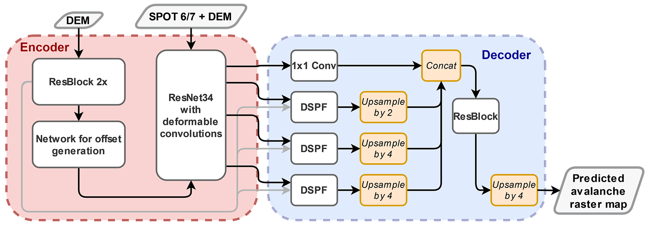
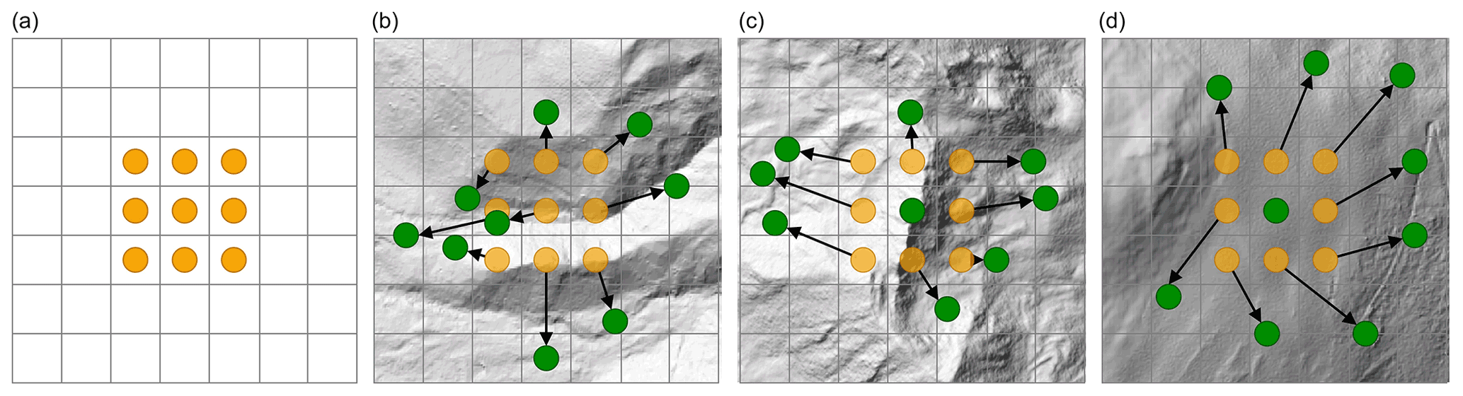
Figure 2For the deformable convolutions, a standard kernel (like the 3×3 as shown in a) will be adapted according to 2D offsets learned from the underlying DEM. The green dots in (b), (c) and (d) exemplarily show possible final positions of the kernel elements; the displacement from the standard kernel is illustrated by the black arrows.
The augmented decoder helps our DeepLabV3+ to propagate features along specific directions, in our case this is the possible downhill flow direction of avalanches which can be extracted from the DEM. Hence, we alter the ASPP such that it aggregates features from all backbone layers and increases the receptive field. The new module, which we call deformable spatial pyramid flow (DSPF, Fig. 4), performs deformable convolutions at different dilation rates. The deformations are again obtained from our small network with offsets, based on the DEM. In order to propagate information along the gradient field, we also model the flow direction of an avalanche in the DSPF module of the decoder.
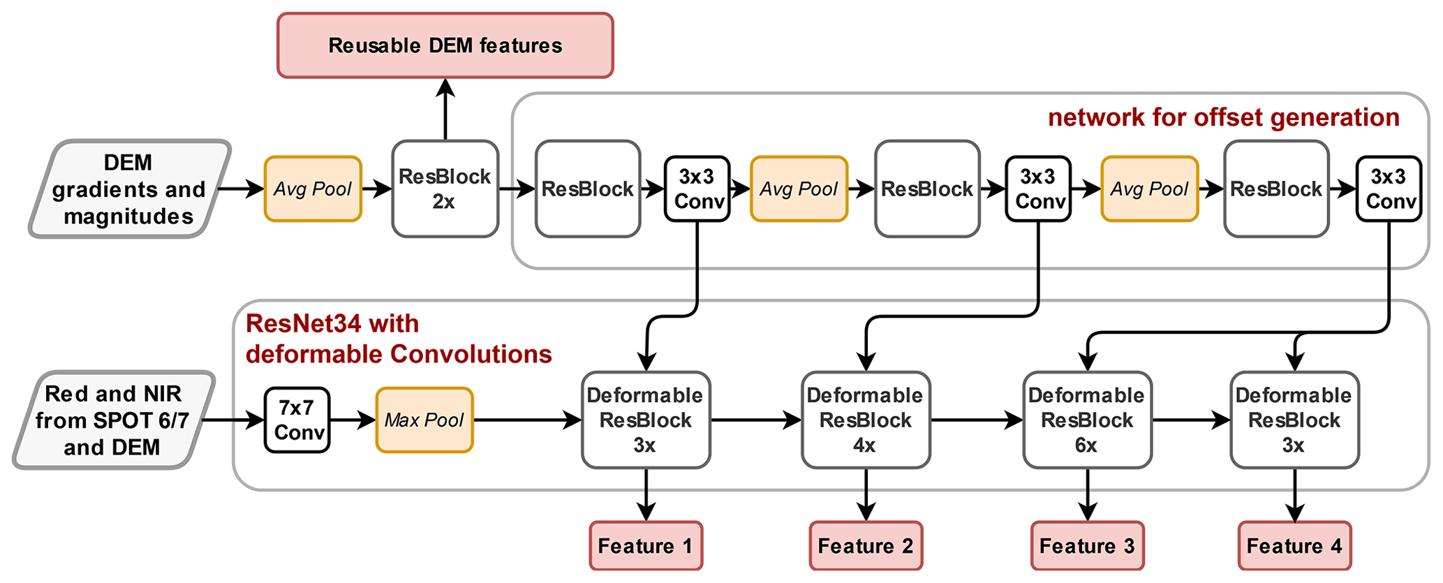
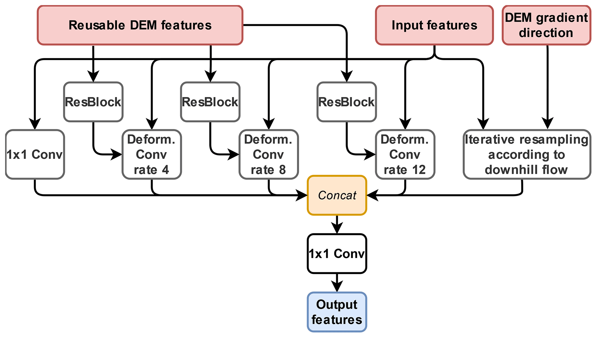
Figure 4Detailed architecture of the deformable spatial pyramid flow (DSPF) used in the decoder of our DeepLabV3+ variant.
3.1.1 Sampling and data split
Given the proposed model architecture and the available computational resources (CPU: 20 Intel Core 3.70 GHz; GPU: 1 NVIDIA GeForce RTX 2080 Ti), we are unable to process an entire orthomosaic at once. Therefore, we process squared image subsets, called patches, of up to 512×512 pixels at training time, which translates into an area of 589 824 m2 at the spatial resolution of SPOT 6/7 imagery. With our model and computational resources we can simultaneously process batches of two image patches per GPU.
For supervised machine learning approaches it is vitally important that all desired classes are present in the patches the model learns from. As classes are usually not evenly distributed, class imbalance is a frequent challenge. Our dataset is very imbalanced: avalanches cover only 11785 of the entire area covered by SPOT 6/7 imagery. Re-balancing of class frequencies is necessary to make sure our model adequately captures the variability of the avalanche class. We use the following pragmatic strategy to ensure a training set that includes relevant examples and with sufficient representation of both classes. First, we iteratively sample patch centers inside manually annotated avalanche polygons while avoiding overlapping patches. In this way, we obtain a set of samples that is not overly imbalanced, with more background pixels than avalanche pixels. These patches form 95 % of our training set. Second, the remaining 5 % are sampled randomly in areas without avalanches to ensure also patches without avalanche pixels are seen during training. This leads to an effective ratio of 1:4 between avalanche and background pixels in the 5185 512×512 patches of the training set.
As the edges of the patches lack context, they were also given smaller weights when calculating the loss function during training, starting 100 pixels from the edge, decreasing the weight linearly to 10 % of the base weight given above at the very edge. For our DeepLabV3+ we additionally used deep supervision as in Simonyan and Zisserman (2015) to help the model converge.
3.1.2 Training
For training and quantitative evaluation, the data were split into mutually exclusive, geographically disjoint regions for training (80 %), validation and hyper-parameter tuning (10 %), and testing (10 %), as depicted in Fig. 5. The test set is located completely in regions acquired either only in 2018 or only in 2019 but not in the overlap between the two acquisitions to prevent memorization (especially of the identical topography).
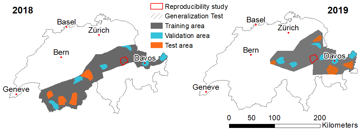
Figure 5Visualization of the disjoint regions for training, validation and testing for both 2018 and 2019. Also shown are the test region for the generalization experiments, where we had additional data from 6 January 2018, and the regions used to study reproducibility of manual avalanche maps.
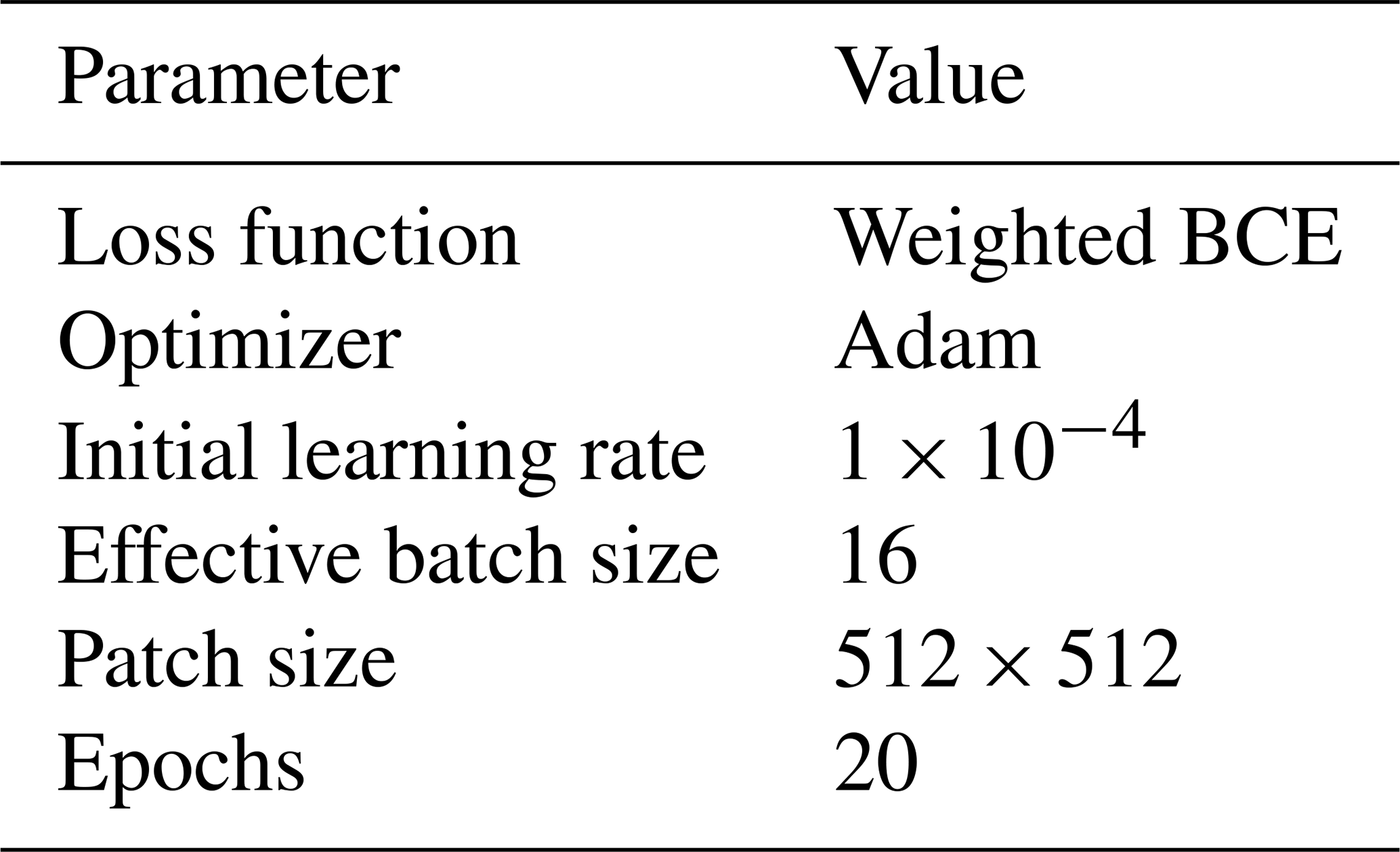
The network is trained by minimizing a weighted binary cross entropy (BCE) loss (see also Sect. 3.1.2), using the Adam optimizer (Kingma and Ba, 2017) for 20 epochs. The base learning rate was initialized to and reduced by a factor of 4 after 10 epochs. A summary of the hyper-parameter settings is given in Table 1.
As a preprocessing step, the input images are normalized channel-wise using the mean and variance values of the entire dataset. Additionally, we flattened the peak in the image histograms caused by the shadow pixels by transforming negative values while keeping positive values unchanged.
Even though our training dataset is large, it covers only two avalanche periods and cannot be expected to account for the whole variety of possible conditions. In order to increase the robustness of the network, we further expand the training set with synthetic data augmentation. We used randomized rotation and flipping for greater topographic variety, mean-shifting and variance-scaling to simulate varying atmosphere and lighting conditions, and patch shifting to increase robustness when only part of an avalanche is visible. To speed up data loading we used batch augmentation (Hoffer et al., 2019), in which the same sample is read only once and used multiple times with different augmentations computed on the fly. To increase the model's performance, we additionally accumulated gradients over two iterations before weights were updated. Thereby an effective batch size of four (2+2) was reached, and the 512×512 pixel patches may be used (see also Sect. 4.2).
As mentioned in Sect. 2 the avalanche polygons come with labels that quantify their visibility in the SPOT data. These labels are used to re-weight their contributions to the BCE loss as follows: pixels on complete, well visible avalanches have weight 2, mostly well visible avalanches, as well as background pixels not on an avalanche, have weight 1, and not completely visible avalanches have weight 0.5.
Predictions are made for a target area specified by vector polygons in the form of shapefiles. To reduce artifacts at the edges of patches, the samples for the predictions overlap by 100 pixels before being cropped. To assess the detection performance of the network, we calculated positive predictive value (PPV, also called precision) and probability of detection (POD, also called recall) on a pixel level, as well as the F1 score. PPV and POD are both based on a standard 2×2 confusion matrix (Trevethan, 2017). As per-pixel metrics take as input a binary mask (avalanche yes or no) and the network yields scores, we thresholded the predictions at 0.5 before calculating statistics and computed the F1 score as
where POD and PPV are defined as
where TP is true positive, FP is false positive, and FN is false negative.
In this paper the presented pixel-wise metrics (POD, PPV and F1 score) represent the average score over all the patches we tested on. As our dataset is imbalanced and the F1 score non-symmetric, we calculated those metrics for both avalanches and the background. Additionally, we wanted to estimate how many avalanches were detected by each model. Consequently, for the object-based metrics we tested two different measures: we counted an avalanche as detected if 50 % or 80 % of all pixels within an avalanche from the manual mapping had a score of 0.5 or higher.
4.1 Results and generalization ability
Results were calculated for the test areas and are reported in Table 2. Compared to the standard DeepLabV3+, our model, when run with the parameters described in Table 1, has a higher POD for avalanches (0.610 vs. 0.587) while having the same PPV. This results in an F1 score of 0.612 for the standard DeepLabV3+ and 0.625 for our version. For the background, the pattern is similar: the POD is slightly better for our method (0.894), compared to the standard DeepLabV3+ (0.888), while the PPV is slightly higher for the standard model (0.900 vs. 0.894). Consequently, the F1 score is very similar as it only differs by one in the third decimal place between our and the standard DeepLabV3+.
For any supervised classification and deep learning methods in particular, the ability to generalize well to new datasets and regions not seen during the training phase is key. To evaluate this, we test our trained model using SPOT 7 imagery from 6 January 2018. The test metrics for predictions on the data from 6 January 2018 were calculated with the standard DeepLabV3+ and the adapted DeepLabV3+. As Table 2 shows, our version generalizes very well (see also Fig. 6); the metrics only differ from tests on the initial dataset in the fourth decimal place. The standard DeepLabV3+, on the other hand, does not generalize so well as the POD, and the detection rates per avalanche are lower than for testing on the initial data.
We also investigated object-based metrics for all model variations: when detection requires 50 % of the avalanche area, the models rightly capture between roughly 58 % and 69 % of all avalanches and between 38 % and 51 % when detection requires 80 % of the area (Table 3). Again the standard DeepLabV3+ performs slightly worse than our adapted DeepLabV3+, especially when run on data from a new avalanche period (6 January 2018). Therefore, our DeeplabV3+ shows better ability to generalize to new and previously unseen data. Overall, the best performance is achieved when considering sunlit avalanche parts only, for both training and testing.
Table 2Segmentation results for the test areas for the standard DeepLabV3+ and our DeepLabV3+, results of predicting on data from a previously unseen avalanche period and variations to our model for the ablation. The metrics shown are the averages from all tested patches. The bold fonts signify the model, data and parameters that were varied compared to what we used as standard in our work.
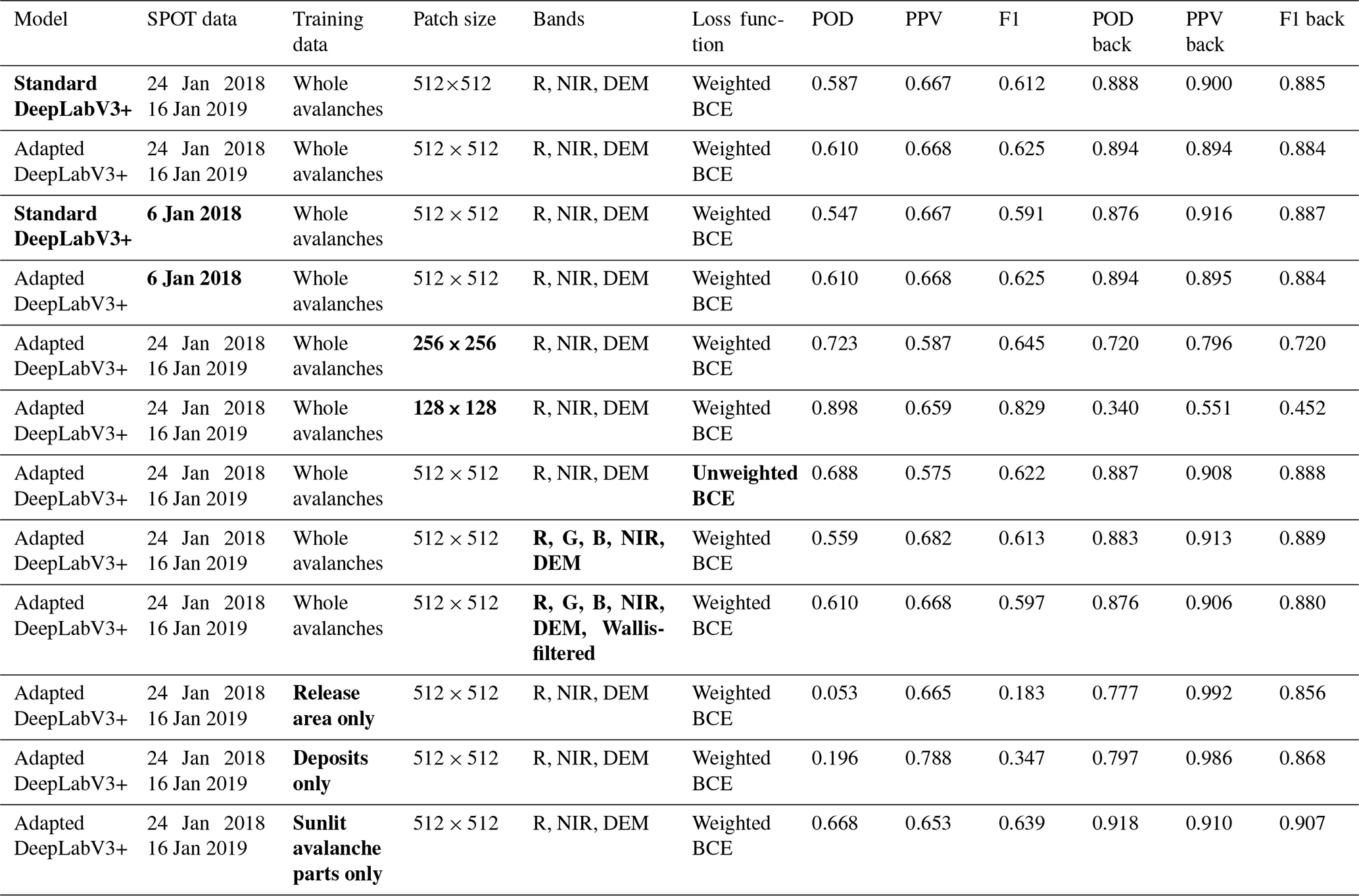
Table 3Object-based metrics for selected model configurations.

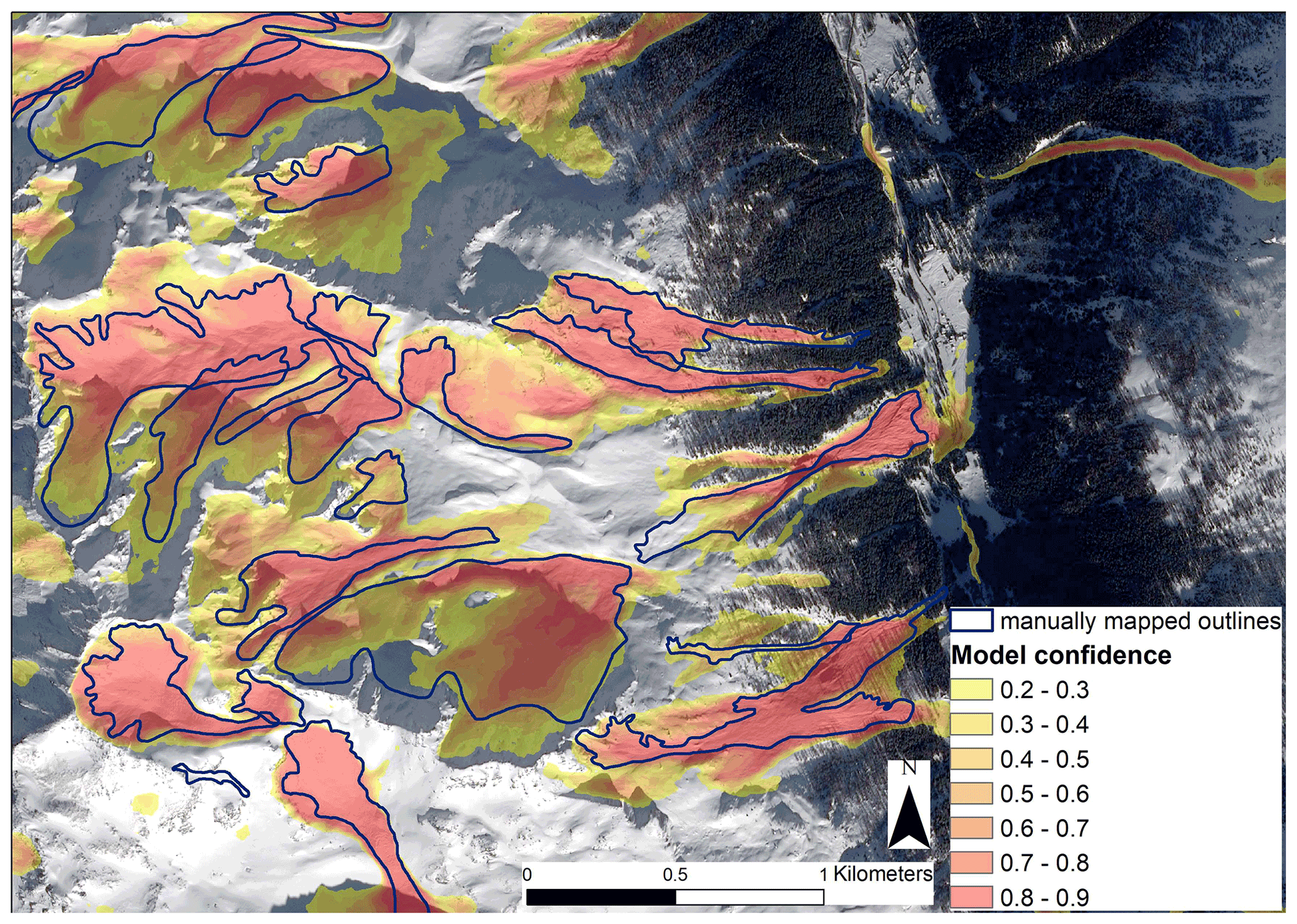
Figure 6An example for the model confidence when predicting on data from a previously unseen avalanche period from 6 January 2018 (SPOT 6 data © Airbus DS 2018). The values closer to 1, in darker hues, indicate places where the model is more confident about the existence of an avalanche. In the illuminated regions those areas almost always overlap with manually mapped avalanches.
4.2 Ablation studies
To understand how our changes to the standard DeepLabV3+ affect performance we varied the model in different ways and trained, tested and compared the performance. These results can be found in Table 2. First, we investigated the influence of the deformable backbone and discovered that including it outperforms the non-deformable backbone configurations of the standard DeepLabV3+. This is the case in our test areas for 2018 and 2019 but also for testing on the avalanche period from 6 January 2018. Secondly, the avalanches in our network have been weighted (see Sect. 3.1.2) according to the quality index assigned by the manual mapper. To quantify the effects of using weights we ran training with unweighted BCE and observed a decrease in POD, a slight increase in PPV and overall a smaller F1 score. Additionally, in our adapted version of DeepLabV3+ we only considered the red and near-infrared from SPOT, as well as the DEM, as input channels. We cannot test the adapted DeepLabV3+ without the DEM as it is explicitly included as an integral part of the network. We analyzed, however, how including all SPOT channels (additionally Blue and Green) and also adding another Wallis filtered channel (to bring out details in the shade) affect network performance (see Table 2). For our model we found that including more channels did not improve the performance; rather training time was longer and metrics worse than with the initial channels.
We hypothesize that the proportion of potential avalanche area and context visible in the patches strongly influences network output. To investigate this, we have trained our model with varying patch sizes: 512×512, 256×256 and 128×128 pixels (corresponding to 768×768, 384×384 and 192×192 m). Quantitative results in Table 2 show the largest patch size performs best considering metrics for both avalanches and background. When comparing them visually (Fig. 7), this is further supported as the predictions on the smallest size are patchy and dispersed over the image, showing the model is unsure about the occurrence of avalanches. With increasing context through a larger patch size though, the model becomes more confident, and the avalanche borders are distinctly visible.
Subsequently, in order to understand what is better for training the network, we trained on avalanche deposits or release areas only. As deposit area, we assumed the lower third (based on elevation) of each manually mapped avalanche, ignoring those avalanches where the deposit had been inferred. For the release areas, we used the zones identified by Bühler et al. (2019), again disregarding those avalanches where the release zone had been inferred and was therefore uncertain. As results in Table 2 show, performance for predicting all avalanches is a lot worse in both cases. We also observe that PPV and POD are significantly higher when the network is trained on deposits only rather than trained only on release areas. This resulted in an increase of 0.146 in F1 score and suggests that the original model might also be learning more from texture-rich avalanche deposits than from release zones.
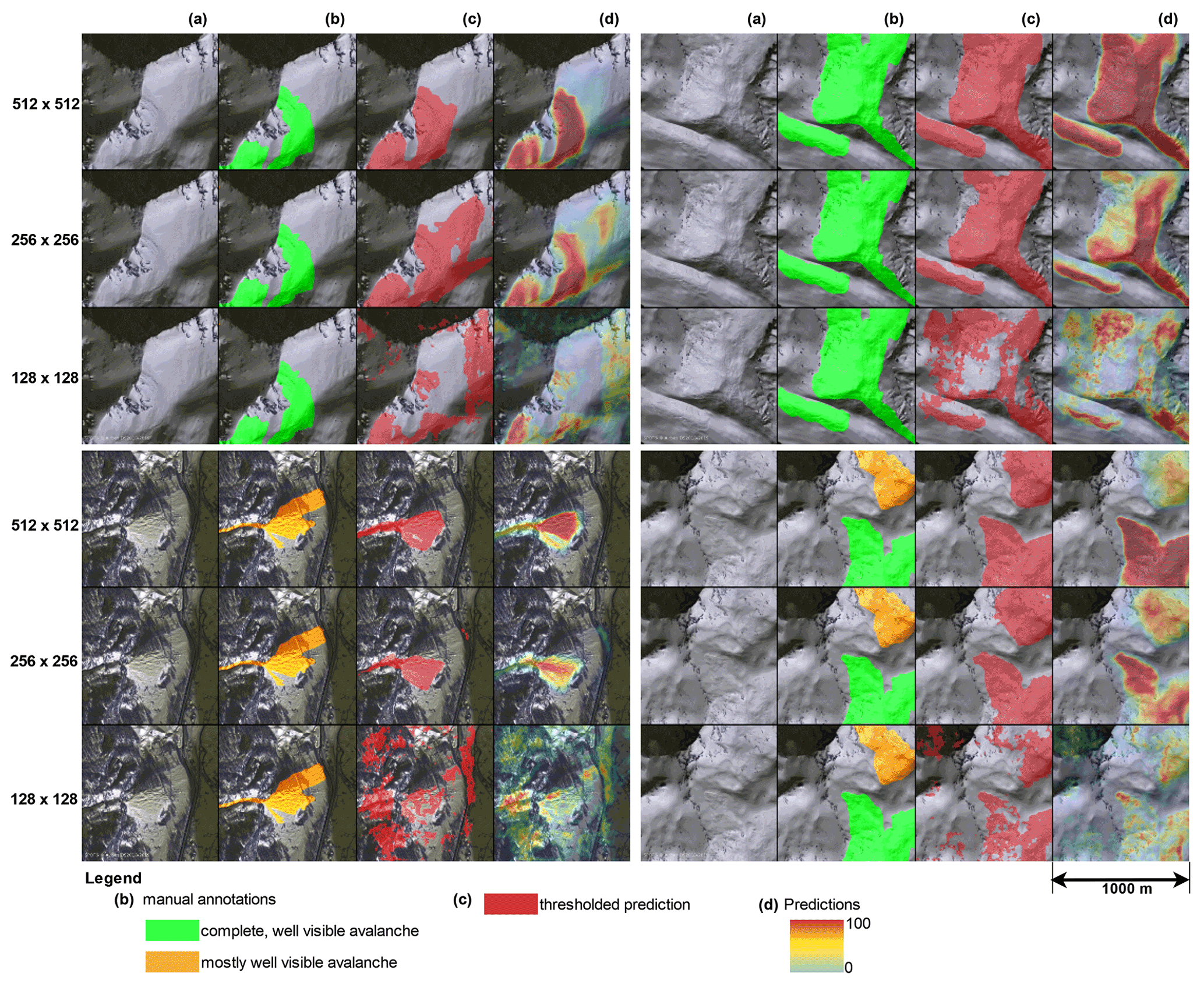
Figure 7Comparison of results for four patches when training the network with different patch sizes. The tiles depict (a) the SPOT 6 image, (b) the manually mapped annotations used as reference, (c) the predictions thresholded at 0.5 and (d) the predicted avalanche probability (SPOT 6 data © Airbus DS 2018). Visual inspections show that the model is a lot more confident the larger the patch size is.
Finally, the experts manually mapping the avalanches generally perceived those in the sun as better visible. Hafner et al. (2021) confirmed that and found the POD to be higher roughly by a factor of 5 for avalanches in fully illuminated terrain compared to those, at the time of image acquisition, in fully shaded terrain. In order to investigate this further, we used a support vector machine (SVM) classifier to calculate a shadow mask for both 2018 and 2019. The mask also includes most forested areas due to their speckled sun–shade pattern. Subsequently, we excluded the avalanche parts located in the shade and trained only with the remaining areas (about one fourth of the avalanche area per year). Calculating the metrics considering only avalanches in illuminated areas, we found an increase of 0.058 in POD, a slight decrease of 0.015 in PPV and consequently an increase in F1 score of 0.014. The object-based metrics (Table 3) are also slightly better when only considering sunlit regions.
4.3 Reproducibility of manually mapped avalanches
To assess the degree of label noise in our dataset, we conducted a reproducibility experiment on the manually mapped avalanches to understand how similar the assessment of a given area by different experts would be. In other fields several comprehensive studies have already been conducted to investigate inter-observer variability, for example, for contouring organs in medical images (Fiorino et al., 1998) or for manual glacier outline identification (Paul et al., 2013). For our investigation five people attempted to replicate the manual mapping with the same methodology as used before and described in detail in Bühler et al. (2019). All five mapping experts are very familiar with satellite imagery and/or avalanches and received the same standardized introductions. The experiment was conducted twice in an area of 90 km2 around Flims, Switzerland, on the 2018 and 2019 SPOT 6/7 imagery (see Fig. 5). The area contains avalanches in the shade and in illuminated terrain, as well as all outline quality classes in the initial mappings (Hafner and Bühler, 2019, 2021). The mapping experts did not see another mapping before having finished theirs.
Table 4F1 scores for the reproducibility investigation: the bold values in the upper-right part of the table represent the scores comparing two expert mappings in illuminated terrain, and the lower-left values are the scores in shaded terrain.
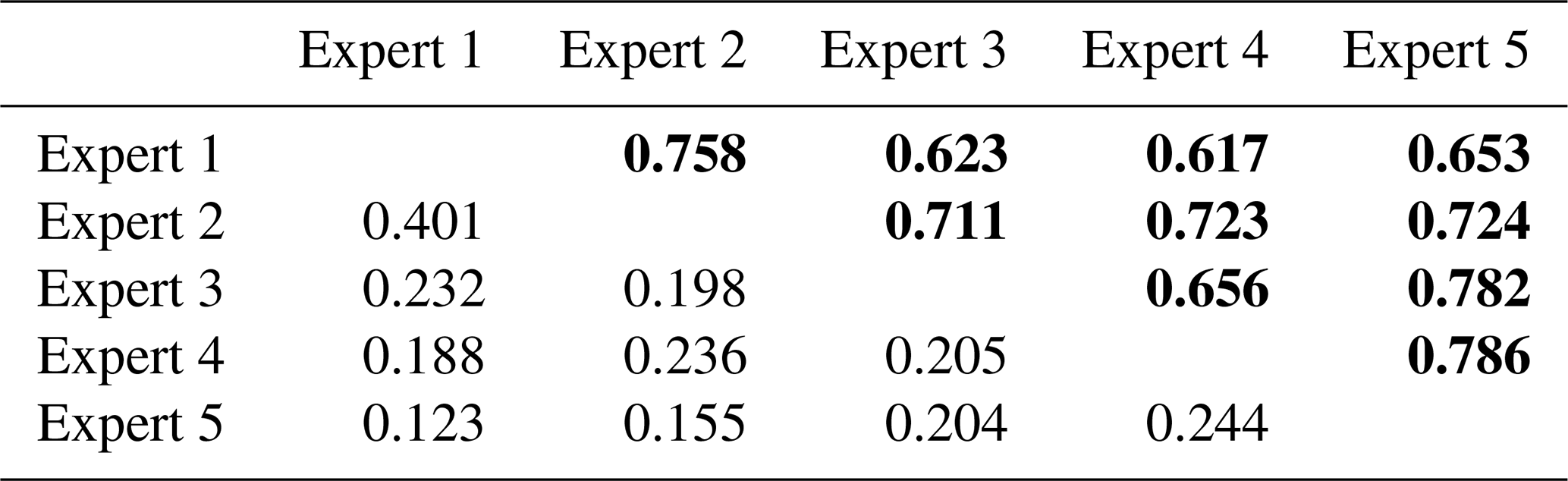
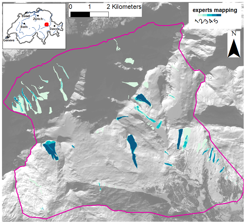
Figure 8Heat map exemplarily illustrating expert agreement on avalanche area for avalanches mapped from SPOT in January 2018 (24 January 2018, SPOT 6 © Airbus DS2018). Agreement in the shade (northern part of the study area) is generally lower than in the sunlit areas to the south. Dark blue indicates very good agreement or in other words marks areas that where identified as an avalanche by all five experts involved. For a more detailed location of the reproducibility study area see Fig. 5.
Calculating F1 score (see Eq. 1) between all experiment mappings, we found an overall F1 score of 0.381 in illuminated and 0.018 in shaded areas (area-wise metrics). Comparing two expert mappings at a time, the values range from 0.617 to 0.786 in the illuminated regions and from 0.123 to 0.401 in the shaded regions of our study area (Table 4). The F1 scores of the expert manual mappings with the initial mapping are in the same range (not shown). The results from 2018 (Fig. 8) illustrate that for some selected avalanches the agreement is very good, while, especially in the shade, there is little agreement among experts on the presence of avalanches.
Reexamining the results from the network now in the light of this experiment, the adapted DeepLabV3+ is equally good as the experts in identifying avalanches. In other words, we cannot expect a computer algorithm to provide better scores than the average F1 score of two mapping experts. Even for the avalanches with the highest agreement, a specific boundary line will usually not match exactly. This makes it hard for any network to learn the localization of boundaries. We do not yet know what exactly causes the differences in avalanche identification between experts. Therefore we plan on conducting a thorough analysis on imagery with different spatial resolutions in the future. This will help us to better understand the inherent mapping uncertainty of avalanches and may give an indication of what performance can be expected if training computational detection algorithms on different optical data.
4.4 Limitations of this study
The three avalanche periods for which we have SPOT imagery all occurred in January. Those images are relatively close to the winter solstice and therefore have a high percentage of shaded area. The amount of shaded area depends very much on the terrain and on the season. Around Davos, Switzerland, for example, 43 % of the area is shaded on the winter solstice but only 7 % 3 months later (both at SPOT 6/7 image acquisition time; Hafner et al., 2021). We know that the quality of the manually annotated avalanches is lower in shaded areas (POD: 0.15 shade, 0.86 illuminated, 0.74 overall; Hafner et al., 2021). Consequently, the training data have lower quality in shaded regions, which makes learning there more difficult for our model and leads to lower model confidence, as well as poorer results. Based on the results when training and testing on sunlit avalanche parts only, however, we see potential for better overall metrics when a smaller portion of the area is shaded closer to the summer solstice. But regardless of how much area is well illuminated, the challenges in the shade remain and make results in those areas less trustworthy. Further research to better understand and tackle that problem is needed.
Additionally, even though 2018 includes wet snow and wet snow avalanches, the snow in January is generally colder and drier than towards the end of the winter. Consequently, we do not know how well our model performs under different snow conditions, for example in spring. Whether our model already generalizes enough or is biased towards high winter conditions and requires retraining with different snow conditions, we could not yet test.
We present a novel deep learning approach for avalanche mapping with deformable convolutions that adapts its notion of the local terrain according to the input digital elevation model (DEM). Experiments at large scale with optical, high-spatial-resolution (1.5 m) SPOT 6/7 satellite imagery show that our approach achieves good performance (F1 score 0.625) and generalizes well to new scenes not seen during the training phase (F1 score 0.625). As reference data for training, validating and testing our model we relied on 24 747 manually mapped and annotated avalanches from two avalanche periods in different years. With our adapted DeepLabV3+ we were able to detect 66% of all avalanches. By varying model parameters and the input data we analyzed the impact of different configurations on the mapping result. We found that weighting the avalanches according to the perceived visibility did result in slightly better metrics than when not weighting them. By training on release areas and deposits only we demonstrated that the network learns more from deposits (Table 2), and by excluding shaded areas from training we showed that in illuminated terrain both training is easier and test results are better (F1 score 0.639). Furthermore, we investigated expert agreement for manual avalanche mapping in a small reproducibility study and found that agreement on avalanche area is substantially lower than expected. Compared to the model, the agreement between experts is in the same range as the adapted DeepLabV3+ performance.
Our work is an important step towards a fast and comprehensive documentation of avalanche periods from optical satellite imagery. This could substantially complement existing avalanche databases, improving their reliability to perform hazard zoning or the planning of mitigation measures. For the future we aim at conducting a more through study investigating expert agreement for manual avalanche identification and its implications for automated avalanche mapping. Additionally, we intend to study the performance of our model on data from different sensors and time periods. Furthermore, we plan on improving results by masking out areas where avalanches cannot occur using, for example, modeled avalanche hazard indication data from Bühler et al. (2022).
The manually mapped avalanche outlines from 24 January 2018 and 16 January 2019 used by us for training, testing and validation are available on EnviDat (Hafner and Bühler, 2019, 2021). The code is available on GitHub: https://github.com/aval-e/DeepLab4Avalanches.git (last access: 22 August 2022) and Zenodo: https://doi.org/10.5281/zenodo.7014498 (Barton and Hafner, 2022).
EDH coordinated the study, performed all initial manual mappings, expanded the neural network code originally implemented by PB and did the statistical analysis. RCD, JDW and KS advised on the machine learning aspects of the project and critically reviewed the associated results. RCD wrote the script for the Wallis filtering. The reproducibility investigation was initiated by KS and coordinated by EDH, and both YB and EDH were part of its mapping team. EDH wrote the manuscript with help from all other authors. EDH and YB originally initiated the automation of avalanche mapping from SPOT.
The contact author has declared that none of the authors has any competing interests.
Publisher's note: Copernicus Publications remains neutral with regard to jurisdictional claims in published maps and institutional affiliations.
We thank Leon Bührle, Benjamin Zweifel and Andreas Stoffel for mapping our reproducibility investigation and Frank Techel for valuable input on its analysis. We are grateful to Edward Bair and the anonymous reviewer for the critical questions, suggestions and comments in their reviews.
This paper was edited by Kang Yang and reviewed by Edward Bair and one anonymous referee.
Abermann, J., Eckerstorfer, M., Malnes, E., and Hansen, B. U.: A large wet snow avalanche cycle in West Greenland quantified using remote sensing and in situ observations, Nat. Hazards, 97, 517–534, https://doi.org/10.1007/s11069-019-03655-8, 2019. a, b
Barton, P. and Hafner, E. D.: aval-e/DeepLab4Avalanches: Code to automatically identify avalanches in SPOT 6/7 imagery (v1.0.0), Zenodo [code], https://doi.org/10.5281/zenodo.7014498, 2022. a
Bebi, P., Kulakowski, D., and Rixen, C.: Snow avalanche disturbances in forest ecosystems – State of research and implications for management, Forest Ecology Manag., 257, 1883–1892, https://doi.org/10.1016/j.foreco.2009.01.050, 2009. a
Bianchi, F. M., Grahn, J., Eckerstorfer, M., Malnes, E., and Vickers, H.: Snow Avalanche Segmentation in SAR Images With Fully Convolutional Neural Networks, IEEE J. Sel. Top. Appl. Earth Obs., 14, 75–82, https://doi.org/10.1109/JSTARS.2020.3036914, 2021. a
Bründl, M. and Margreth, S.: Integrative Risk Management, in: Snow and Ice-Related Hazards, edited by: Haeberli, W. and Whiteman, C., Risks Disast., 2015, 263–301, https://doi.org/10.1016/B978-0-12-394849-6.00009-3, 2015. a
Bühler, Y., Hüni, A., Christen, M., Meister, R., and Kellenberger, T.: Automated detection and mapping of avalanche deposits using airborne optical remote sensing data, Cold Reg. Sci. Technol., 57, 99–106, https://doi.org/10.1016/j.coldregions.2009.02.007, 2009. a, b
Bühler, Y., Hafner, E. D., Zweifel, B., Zesiger, M., and Heisig, H.: Where are the avalanches? Rapid SPOT6 satellite data acquisition to map an extreme avalanche period over the Swiss Alps, The Cryosphere, 13, 3225–3238, https://doi.org/10.5194/tc-13-3225-2019, 2019. a, b, c, d, e, f, g, h, i
Bühler, Y., Bebi, P., Christen, M., Margreth, S., Stoffel, L., Stoffel, A., Marty, C., Schmucki, G., Caviezel, A., Kühne, R., Wohlwend, S., and Bartelt, P.: Automated avalanche hazard indication mapping on a statewide scale, Nat. Hazards Earth Syst. Sci., 22, 1825–1843, https://doi.org/10.5194/nhess-22-1825-2022, 2022. a, b
Cai, Y., Guan, K., Peng, J., Wang, S., Seifert, C., Wardlow, B., and Li, Z.: A high-performance and in-season classification system of field-level crop types using time-series Landsat data and a machine learning approach, Remote Sens. Environ., 210, 35–47, https://doi.org/10.1016/j.rse.2018.02.045, 2018. a
Chen, L., Zhu, Y., Papandreou, G., Schroff, F., and Adam, H.: Encoder-Decoder with Atrous Separable Convolution for Semantic Image Segmentation, CoRR, abs/1802.02611, http://arxiv.org/abs/1802.02611 (last access: 22 August 2022), 2018. a, b, c
Christen, M., Kowalski, J., and Bartelt, P.: RAMMS: Numerical simulation of dense snow avalanches in three-dimensional terrain, Cold Reg. Sci. Technol., 63, 1–14, https://doi.org/10.1016/j.coldregions.2010.04.005, 2010. a
Dai, J., Qi, H., Xiong, Y., Li, Y., Zhang, G., Hu, H., and Wei, Y.: Deformable Convolutional Networks, in: 2017 IEEE International Conference on Computer Vision (ICCV), 764–773, https://doi.org/10.1109/ICCV.2017.89, 2017. a, b
Eckerstorfer, M., Bühler, Y., Frauenfelder, R., and Malnes, E.: Remote sensing of snow avalanches: Recent advances, potential, and limitations, Cold Reg. Sci. Technol., 121, 126–140, https://doi.org/10.1016/j.coldregions.2015.11.001, 2016. a, b
Eckerstorfer, M., Vickers, H., Malnes, E., and Grahn, J.: Near-Real Time Automatic Snow Avalanche Activity Monitoring System Using Sentinel-1 SAR Data in Norway, Remote Sensing, 11, 2863, https://doi.org/10.3390/rs11232863, 2019. a
Eckerstorfer, M., Oterhals, H., Müller, K., Malnes, E., Grahn, J., Langeland, S., and Velsand, P.: Performance of manual and automatic detection of dry snow avalanches in Sentinel-1 SAR images, Cold Reg. Sci. Technol., 198, 103549, https://doi.org/10.1016/j.coldregions.2022.103549, 2022. a, b
Fiorino, C., Reni, M., Bolognesi, A., and Calandrino, R.: Intra- and inter-observer variability in contouring prostate and seminal vesicles: Implications for conformal treatment planning, Radiother. Oncol., 47, 285–292, https://doi.org/10.1016/S0167-8140(98)00021-8, 1998. a
Hafner, E. and Bühler, Y.: SPOT6 Avalanche outlines 24 January 2018, EnviDat [data set], https://doi.org/10.16904/envidat.77, 2019. a, b, c, d
Hafner, E. D. and Bühler, Y.: SPOT6 Avalanche outlines 16 January 2019, EnviDat [data set], https://doi.org/10.16904/envidat.235, 2021. a, b, c, d
Hafner, E. D., Techel, F., Leinss, S., and Bühler, Y.: Mapping avalanches with satellites – evaluation of performance and completeness, The Cryosphere, 15, 983–1004, https://doi.org/10.5194/tc-15-983-2021, 2021. a, b, c, d, e, f, g, h, i, j
Hamar, J. B., Salberg, A.-B., and Ardelean, F.: Automatic detection and mapping of avalanches in SAR images, in: 2016 IEEE International Geoscience and Remote Sensing Symposium (IGARSS), 689–692, https://doi.org/10.1109/IGARSS.2016.7729173, 2016. a
He, K., Zhang, X., Ren, S., and Sun, J.: Deep Residual Learning for Image Recognition, in: 2016 IEEE Conference on Computer Vision and Pattern Recognition (CVPR), pp. 770–778, https://doi.org/10.1109/CVPR.2016.90, 2016. a, b
Hoffer, E., Ben-Nun, T., Hubara, I., Giladi, N., Hoefler, T., and Soudry, D.: Augment your batch: better training with larger batches, arXiv, https://doi.org/0.48550/ARXIV.1901.09335, 2019. a
Karbou, F., Coléou, C., Lefort, M., Deschatres, M., Eckert, N., Martin, R., Charvet, G., and Dufour, A.: Monitoring avalanche debris in the French mountains using SAR observations from Sentinel-1 satellites, International Snow Science Workshop ISSW, Innsbruck, pp. 344–347, 2018. a
Kingma, D. P. and Ba, J.: Adam: A Method for Stochastic Optimization, 2017. a
Kingma, D. P. and Welling, M.: An Introduction to Variational Autoencoders, CoRR, abs/1906.02691, http://arxiv.org/abs/1906.02691 (last access: 22 August 2022), 2019. a
Korzeniowska, K., Bühler, Y., Marty, M., and Korup, O.: Regional snow-avalanche detection using object-based image analysis of near-infrared aerial imagery, Nat. Hazards Earth Syst. Sci., 17, 1823–1836, https://doi.org/10.5194/nhess-17-1823-2017, 2017. a, b
Lato, M. J., Frauenfelder, R., and Bühler, Y.: Automated detection of snow avalanche deposits: segmentation and classification of optical remote sensing imagery, Nat. Hazards Earth Syst. Sci., 12, 2893–2906, https://doi.org/10.5194/nhess-12-2893-2012, 2012. a, b
Ma, L., Liu, Y., Zhang, X., Ye, Y., Yin, G., and Johnson, B. A.: Deep learning in remote sensing applications: A meta-analysis and review, ISPRS J. Photogramm., 152, 166–177, https://doi.org/10.1016/j.isprsjprs.2019.04.015, 2019. a
Meister, R.: Country-wide Avalanche Warning in Switzerland, International Snow Science Workshop ISSW, Snowbird, Utah, USA, 58–71, 1994. a
OpenTopography: Shuttle Radar Topography Mission (SRTM) Global, OpenTopography, https://doi.org/10.5069/G9445JDF, 2013. a
Paul, F., Barrand, N., Baumann, S., Berthier, E., Bolch, T., Casey, K., Frey, H., Joshi, S., Konovalov, V., Le Bris, R., Mölg, N., Nosenko, G., Nuth, C., Pope, A., Racoviteanu, A., Rastner, P., Raup, B., Scharrer, K., Steffen, S., and Winsvold, So. H.: On the accuracy of glacier outlines derived from remote-sensing data, Ann. Glaciol., 54, 171–182, https://doi.org/10.3189/2013AoG63A296, 2013. a
Prakash, N., Manconi, A., and Loew, S.: A new strategy to map landslides with a generalized convolutional neural network, Sci. Rep.-UK, 11, 1–15, 2021. a
Robson, B. A., Bolch, T., MacDonell, S., Hölbling, D., Rastner, P., and Schaffer, N.: Automated detection of rock glaciers using deep learning and object-based image analysis, Remote Sens. Environ., 250, 112033, https://doi.org/10.1016/j.rse.2020.112033, 2020. a
Ronneberger, O., Fischer, P., and Brox, T.: U-Net: Convolutional Networks for Biomedical Image Segmentation, in: Medical Image Computing and Computer-Assisted Intervention – MICCAI 2015, Springer International Publishing, Cham, 234–241, 2015. a, b
Rudolf-Miklau, F., Sauermoser, S., and Mears, A. (Eds.): The technical avalanche protection handbook, Ernst & Sohn, Berlin, ISBN 978-3-433-03034-9, 2015. a
Simonyan, K. and Zisserman, A.: Very Deep Convolutional Networks for Large-Scale Image Recognition, arXiv, https://doi.org/10.48550/arXiv.1409.1556, 2015. a, b
Sinha, S., Giffard-Roisin, S., Karbou, F., Deschatres, M., Karas, A., Eckert, N., Coléou, C., and Monteleoni, C.: Can Avalanche Deposits be Effectively Detected by Deep Learning on Sentinel-1 Satellite SAR Images?, in: Climate Informatics, Paris, France, https://hal.archives-ouvertes.fr/hal-02278230 (last access: 22 August 2022), 2019a. a
Sinha, S., Giffard-Roisin, S., Karbou, F., Deschatres, M., Karas, A., Eckert, N., and Monteleoni, C.: Detecting Avalanche Deposits using Variational Autoencoder on Sentinel-1 Satellite Imagery, in: NeurIPS 2019 Workshop: Tackling Climate Change with Machine Learning NeurIPS workshop, Vancouver, Canada, https://hal.archives-ouvertes.fr/hal-02318407 (last access: 22 August 2022), 2019b. a
Sun, K., Zhao, Y., Jiang, B., Cheng, T., Xiao, B., Liu, D., Mu, Y., Wang, X., Liu, W., and Wang, J.: High-Resolution Representations for Labeling Pixels and Regions, ArXiv, https://doi.org/10.48550/ARXIV.1904.04514, 2019. a
swisstopo: swissALTI3D – Das hoch aufgelöste Terrainmodell der Schweiz, https://www.swisstopo.admin.ch/content/swisstopo-internet/de/geodata/height/alti3d/_jcr_content/contentPar/tabs_copy/items/dokumente/tabPar/downloadlist/downloadItems/846_1464690554132.download/swissALTI3D_detaillierte Produktinfo_DE_bf.pdf (last access: 20 August 2022), 2018. a
Trevethan, R.: Sensitivity, Specificity, and Predictive Values: Foundations, Pliabilities, and Pitfalls in Research and Practice, Front. Pub. He., 5, 307, https://doi.org/10.3389/fpubh.2017.00307, 2017. a
Waldeland, A. U., Reksten, J. H., and Salberg, A.-B.: Avalanche Detection in SAR Images Using Deep Learning, in: IGARSS 2018–2018 IEEE International Geoscience and Remote Sensing Symposium, 2386–2389, https://doi.org/10.1109/IGARSS.2018.8517536, 2018. a
Wesselink, D. S., Malnes, E., Eckerstorfer, M., and Lindenbergh, R. C.: Automatic detection of snow avalanche debris in central Svalbard using C-band SAR data, Polar Res., 36, 1333236, https://doi.org/10.1080/17518369.2017.1333236, 2017. a
WSL Institute for Snow and Avalanche Research SLF (Ed.): Avalanche Bulletin Interpretation Guide, WSL Institute for Snow and Avalanche Research SLF, Edition November 2021, 53 pp., https://www.slf.ch/files/user_upload/SLF/Lawinenbulletin_Schneesituation/Wissen_zum_Lawinenbulletin/Interpretationshilfe/Interpretationshilfe_EN.pdf (last access: 22 August 2022), 2021. a, b