the Creative Commons Attribution 4.0 License.
the Creative Commons Attribution 4.0 License.
 | 26 Jan 2022
Satellite passive microwave sea-ice concentration data set intercomparison using Landsat data
Thomas Lavergne
Leif Toudal Pedersen
Rasmus Tage Tonboe
Louisa Bell
Maybritt Meyer
Luise Zeigermann
We report on results of an intercomparison of 10 global sea-ice concentration (SIC) data products at 12.5 to 50.0 km grid resolution from satellite passive microwave (PMW) observations. For this we use SIC estimated from >350 images acquired in the visible–near-infrared frequency range by the joint National Aeronautics and Space Administration (NASA) and United States Geological Survey (USGS) Landsat sensor during the years 2003–2011 and 2013–2015. Conditions covered are late winter/early spring in the Northern Hemisphere and from late winter through fall freeze-up in the Southern Hemisphere. Among the products investigated are the four products of the European Organisation for the Exploitation of Meteorological Satellites (EUMETSAT) Ocean and Sea Ice Satellite Application Facility (OSI SAF) and European Space Agency (ESA) Climate Change Initiative (CCI) algorithms SICCI-2 and OSI-450. We stress the importance to consider intercomparison results across the entire SIC range instead of focusing on overall mean differences and to take into account known biases in PMW SIC products, e.g., for thin ice. We find superior linear agreement between PMW SIC and Landsat SIC for the 25 and the 50 km SICCI-2 products in both hemispheres. We discuss quantitatively various uncertainty sources of the evaluation carried out. First, depending on the number of mixed ocean–ice Landsat pixels classified erroneously as ice only, our Landsat SIC is found to be biased high. This applies to some of our Southern Hemisphere data, promotes an overly large fraction of Landsat SIC underestimation by PMW SIC products, and renders PMW SIC products overestimating Landsat SIC particularly problematic. Secondly, our main results are based on SIC data truncated to the range 0 % to 100 %. We demonstrate using non-truncated SIC values, where possible, can considerably improve linear agreement between PMW and Landsat SIC. Thirdly, we investigate the impact of filters often used to clean up the final products from spurious SIC over open water due to weather effects and along coastlines due to land spillover. Benefiting from the possibility to switch on or off certain filters in the SICCI-2 and OSI-450 products, we quantify the impact land spillover filtering can have on evaluation results as shown in this paper.
- Article
(5033 KB) - Full-text XML
-
Supplement
(7024 KB) - BibTeX
- EndNote


We carry on the evaluation of sea-ice concentration (SIC) products derived from satellite passive microwave (PMW) observations. In Kern et al. (2019), we presented an evaluation of 10 PMW SIC products at 0 % and 100 % SIC and with respect to sea-ice observations along ship tracks. Another study focused on Arctic summer conditions, investigating the bias between these PMW SIC products and independent SIC and net ice surface fraction estimates based on MODerate resolution Imaging Spectroradiometer (MODIS) observations (Kern et al., 2020b). With this study, we shift our focus more towards intermediate SIC and utilize a much larger and, partly, more accurate reference data set than in the two earlier studies. The evaluation at 0 % SIC in Kern et al. (2019) utilized a few fixed open water locations only. The evaluation at 100 % SIC used near-100 % SIC estimates based on the analysis of freezing-season synthetic aperture radar (SAR) image pairs representing convergent ice motion coinciding with a complete ice coverage and therefore a high probability to encounter near-100 % SIC. Thus, we evaluated the PMW SIC products for one specific set of ice conditions only (winter and near-100 %). Kern et al. (2019) also presented results of an evaluation of PMW SIC against a multi-annual set of standardized manual visual ship-based observations of the ice conditions. These observations are, however, of limited accuracy and of limited representativity because the average accuracy is between 5 % and 10 %, and observations mostly represent sea-ice conditions where it is possible to navigate. In addition, to reduce noise, PMW and ship-based SIC were averaged over all observations along a ship-track within 1 d, representing sea-ice conditions across spatial scales that – in the worst case – vary by an order of magnitude. The averaging resulted in a reduction in the number of valid data pairs from approximately 15 000 to less than 800, i.e., about 400 per hemisphere.
Another aspect is that the accuracy of the hemispheric but also the regional sea-ice area (SIA) computed from PMW SIC estimates strongly depends on their accuracy. PMW SIC values biased high yield an overestimation of the SIA, whereas PMW SIC biased low results in an underestimation of the SIA. This seems not to be critical as long as the trend is correct (e.g., Ivanova et al., 2014) but limits the use of such SIA estimates for quantitative intercomparisons of climate model results against observations (e.g., Burgard et al., 2020). It is definitely important PMW SIC is 100 % where the actual SIC is 100 % to avoid artificially elevated ocean–atmosphere heat fluxes when used as a surface forcing. It is equally important PMW SIC is an accurate estimate of the open water fraction, hence providing 95 % where the actual SIC is 95 % due to leads and openings in the sea-ice cover. In addition, it is desirable to check the performance of PMW SIC products across the entire SIC range in order to have a reliable estimate of the actual ice cover in, for example, the marginal ice zone (MIZ). Here gradients in heat fluxes are often particularly large. A correct definition of and accurate SIC distribution within the MIZ are also crucial should SIC values be used to evaluate numerical models capable to simulate wave–sea ice interaction (e.g., Boutin et al., 2020; Nose et al., 2020). The ship-based SIC observations used in Kern et al. (2019) offer only limited potential to carry out this performance check because of the above-mentioned reasons, the small number of observations falling into the relevant SIC range of, e.g., 20 % to 80 %, and the larger observational error in this SIC range.
Therefore, in this paper we focus on the evaluation of PMW SIC products against a large number of high-resolution binary sea-ice cover maps estimated from satellite observations acquired in the visible frequency range by NASA–USGS Landsat-5, Landsat-7, and Landsat-8. Overall, we used over 350 such Landsat-based maps, corresponding to more than 10 000 25 km×25 km resolution PMW SIC grid cells. We chose Landsat over MODIS because of the substantially finer spatial resolution of the visible channels of Landsat: 30 m compared to MODIS' 250 m. We note in this context that several studies used MODIS visible–near-infrared observations to either evaluate or complement PMW SIC products (e.g., Ludwig et al., 2020; Shi et al., 2021). Another option would have been to use Sentinel-2's MultiSpectral Instrument (MSI) (Drusch et al., 2012). We discarded this option in light of the limited overlap between this satellite mission (Sentinel-2A was launched June 2015) and our PMW SIC data set, but it will be very valuable in the future since it will allow the data set to be extended to areas much further from land and will likely provide an even more accurate evaluation data set.
Utilization of the high-resolution information provided by Landsat as a means for assessing satellite PMW SIC products dates back to the early 1980s when Comiso and Zwally (1982) compared Nimbus-7 Scanning Multichannel Microwave Radiometer (SMMR) SIC with Landsat imagery. Since then a number of studies have used a small number of such images for SIC intercomparison and/or evaluation (e.g., Steffen and Maslanik, 1988; Steffen and Schweiger, 1991; Comiso and Steffen, 2001; Cavalieri et al., 2006; Wiebe et al., 2009; Lu et al., 2018; Zhao et al., 2021). Landsat imagery has also recently been used for quality assessment of SIC estimates from Suomi National Polar-Orbiting Partnership Visible Infrared Imaging Radiometer Suite (NPP VIIRS) observations (e.g., Liu et al., 2016). Common to all these studies is that they used a comparably small number of Landsat scenes, i.e., less than 10, an order of magnitude smaller than the 368 scenes used in this study (see above).
Analysis of visible satellite imagery for SIC estimation is quite straightforward. A threshold-based method discriminating between open water and ice is applied at the native spatial resolution (pixel size: 30 m×30 m) of the Landsat channels in the visible frequency range, assuming that a pixel is covered by either ice or water. Co-locating this high-resolution information of the binary ice–water distribution with the coarse-resolution PMW SIC products and counting ice and water pixels within a PMW SIC product's grid cell provide an adequate independent measure of the SIC. We refer to Sect. 2.2 for more details.
For evaluating the PMW SIC products across the SIC range, we prefer to use visible data instead of SAR data. The main advantages of SAR data would be the larger area covered by a single scene compared to Landsat (about 400 to 500 km in SAR wide-swath mode (WSM) vs. 180 km for Landsat) and their independence from daylight and cloud cover. In fact, many PMW SIC intercomparison studies have already used SAR images (e.g., Comiso et al., 1991; Dokken et al., 2000; Belchansky and Douglas, 2002; Kwok, 2002; Heinrichs et al., 2006; Andersen et al., 2007; Wiebe et al., 2009; Han and Kim, 2018). However, despite the past decade's substantial progress in developing and testing methods to translate SAR images into high-resolution SIC maps (e.g., Cooke and Scott, 2019; Karvonen, 2014, 2017; Komarov and Buehner, 2017, 2019; Leigh et al., 2014; Lohse et al., 2019; Ochilov and Clausi, 2012; Singha et al., 2018; Wang et al., 2016, 2017; Zakhvatkina et al., 2017; Boulze et al., 2020; Malmgren-Hansen et al., 2020; Wang and Li, 2021), some using machine learning approaches, the accuracy of the obtained SIC maps is not always satisfactory. Particularly at intermediate SIC – the main focus of this study – SAR signatures are often ambiguous, resulting in SAR SIC uncertainties too large for our purposes. Furthermore, applications of such methods to derive Southern Ocean SIC from SAR are comparably sparse. Therefore, we do not use SAR-based SIC maps.
We note that also Ice charting services (FMI, DMI, MET Norway, CIS, NATICE, AARI) heavily depend on SAR imagery for production of their ice charts. They thus have a large demand to automate processes of classification and are potentially most advanced in testing automated SAR SIC retrieval (e.g., Cheng et al., 2020). However, ice charts provide SIC ranges within polygons that are highly variable and heterogeneous in size and shape. Several studies used such ice charts for various intercomparison purposes (e.g., Shokr and Markus, 2006; Shokr and Agnew, 2013; Titchner and Rayner, 2014). Some centers providing operational sea-ice information also use such charts for routine quality checking of PMW SIC products. However, for our purpose of evaluating PMW SIC climate data records (CDRs) and similar SIC products, the limitations of such charts in terms of precision and accuracy – particularly in the intermediate SIC range (e.g., Cheng et al., 2020) – exclude their usage in this study.
After this introduction, this paper provides information about the PMW SIC products, the Landsat data set used, and the methods applied to derive SIC from the Landsat images (Sect. 2). We present our results in Sects. 3 and 4, discuss some additional aspects in Sect. 5, and conclude the study in Sect. 6.
2.1 Sea-ice concentration data sets
The 10 different PMW SIC products considered in our study are summarized briefly in Table 1. We refrain from repeating information about the algorithms themselves, tie point selection, application of weather filters, consideration of land spillover effects, and so forth. All this information is provided in detail in Lavergne et al. (2019), Kern et al. (2019, their Appendix 7.1–7.6), and Kern et al. (2020b). The same applies to the fact that four of the products (SICCI-12km, SICCI-25km, SICCI-50km, and OSI-450) allow us to take into account the full SIC distribution at 0 % and 100 %. Such a distribution is the natural result of the SIC retrieval method used in all SIC products considered – except Nasa Team 2 (NT2). This distribution contains negative as well as SIC values above 100 % that are typically truncated, i.e., set to exactly 0 % and 100 %. We refer to Lavergne et al. (2019) and Kern et al. (2019) for more information in this regard.
Table 1Overview of the investigated PMW SIC products. Column “ID (algorithm)” holds the identifier we use henceforth to refer to the data product and which algorithm it uses. For those algorithms for which an AMSR sensor forms part of the name, we refer to AMSR-E or AMSR2, depending on the respective data used; we write AMSR if we refer to products from both satellites. Column “Input data” refers to the input satellite data for the data set, together with the frequencies and respective field-of-view dimensions.

In order to extend the time series of the Comiso bootstrap (CBT) algorithm and the NT2 algorithm using Advanced Microwave Scanning Radiometer aboard Earth Observation Satellite (AMSR-E) data beyond AMSR-E's capabilities to provide daily maps of the polar regions (3 October 2011), we use the respective unified product based on data from the Advanced Microwave Scanning Radiometer aboard GCOM-W1 (Global Change Observation Mission-Water): AMSR2 (Meier et al., 2018). With that we use five products based on AMSR-E and AMSR2 data and five products based on Special Sensor Microwave/Imager (SSM/I) and Special Sensor Microwave Imager and Sounder (SSMIS) data of the period 2002 through 2015. We do not use PMW SIC data from the period October 2011 through July 2012 because of the gap between AMSR-E and AMSR2. All PMW SIC data have daily temporal resolution. The grid type and grid resolution of all data sets is shown in Table 1. We estimate the Landsat SIC (see Sect. 2.2) at the grid resolution of the respective product. We chose the 25 km grid resolution version of the AMSR-E and AMSR2 products because this resolution is closer to the footprint sizes of the involved channels, and this is the resolution of the respective SSM/I and SSMIS versions of these products. We use version 3 of the NOAA/NSIDC SIC CDR (Peng et al., 2013; Meier et al., 2017) even though version 4 has been released (Meier et al., 2021) because we want to be consistent with the two previous papers (Kern et al., 2019, 2020b).
2.2 The Landsat data set
We use Landsat data of the Thematic Mapper (TM) on Landsat-5, the Enhanced Thematic Mapper (ETM) on Landsat-7, and the Operational Land Imager (OLI) on Landsat-8 obtained in level 1c GeoTIFF format from https://earthexplorer.usgs.gov (last accessed: 28 June 2021) for the years 2003–2011 (Landsat-5), 2003 (Landsat-7), and 2013–2015 (Landsat-8). We downloaded only images with a cloud fraction <30 % provided as a search criterion upfront. In the Northern Hemisphere, we use images of the months of March, April, May, and September, i.e., from late winter to spring and at the onset of fall freeze-up; in the Southern Hemisphere we use images of the months of October through March, i.e., from late winter over summer to fall freeze-up. The total number of images acquired is 421; these split into 152, 12, and 227 for Landsat-5, Landsat-7, and Landsat-8, respectively, and partition into 259 images for the Northern Hemisphere and 162 images for the Southern Hemisphere.
2.2.1 Processing
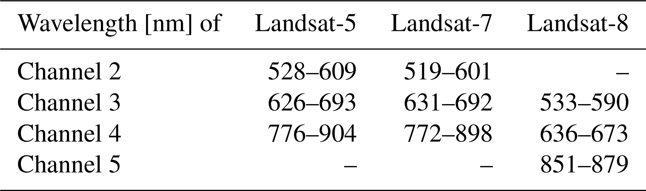
We compute the top of atmosphere (TOA) reflectance for channels 2 to 4 (Landsat-5 and Landsat-7) or channels 3 to 5 (Landsat-8) following Chander et al. (2007, 2009) and USGS (2019). Table 2 provides the wavelengths of these channels (e.g., Chander et al., 2009; Barsi et al., 2014). The solar zenith angle and other parameters required for this computation are either included in the Landsat data files or are taken from Chander et al. (2007, 2009) and the Landsat 8 data users handbook (USGS, 2019). To convert the TOA reflectances to surface reflectances or surface albedo we follow the approaches of Koepke (1989) and Knap et al. (1999). They assume that the TOA reflectance (or planetary reflectance) equals the TOA albedo (or planetary albedo) and that the TOA albedo αTOA is related to the surface albedo αsurface via the simple linear relationship:
The coefficients a and b are a function of the atmospheric conditions, the solar zenith angle, and the wavelength. We follow Koepke (1989) and take values for a and b from his Figs. 1 (KF1) and 2 (KF2). We use KF1 derived for the Advanced Very High Resolution Radiometer (AVHRR) channel 1 for Landsat channels in the wavelength range 500–700 nm. We use KF2 derived for AVHRR channel 2 for Landsat channels in the wavelength range 700–900 nm. We choose those atmospheric conditions that are appropriate for a polar marine atmosphere. For aerosol optical depth we use 0.05, for ozone content we use 0.24 cm NTP (NTP stands for normal temperature and pressure) corresponding to 240 Dobson units, and for water vapor content we use 0.5 g cm−2. Using Eq. (1) we convert TOA albedo into surface albedo values separately for the three channels of the respective Landsat instrument. Subsequently, we compute from these surface albedo values an estimate of the surface broadband shortwave albedo (e.g., Brandt et al., 2005) using the bandwidths of the channels as weights (see Table 2).
Table 2Overview about the wavelengths and bandwidths of the Landsat channels used.
For every broadband surface albedo map, we perform a supervised visual classification into open water, bare/thin ice, and thick/snow-covered ice. For that, we assume the respective surface class covers a Landsat pixel entirely. We assign all dark pixels (with an albedo of, on average, smaller than 0.06) to the open water class. We assign all bright pixels (with an albedo of, on average, larger than 0.45) to the class thick/snow-covered ice; all remaining pixels fall into the class bare/thin ice. We pay more attention separating open water from ice very accurately than distinguishing between bare/thin ice and thick/snow-covered ice. In every Landsat albedo map we search for leads or openings, zoom into these, and perform histogram-equalized slicing to visually identify – based on albedo values and spatial structures – whether the leads or openings selected contain open water. We take the threshold value chosen to separate open water from ice from Pegau and Paulsen (2001). The threshold value chosen to distinguish between bare/thin ice and thick/snow-covered ice is based on Brandt et al. (2005) and Zatko and Warren (2015). They found an albedo of around 0.33 for bare thin ice less than 30 cm thick and of around 0.42 for snow-covered thin ice (5–10 cm thick) with a thin (<3 cm) snow cover. Note that the actual threshold values chosen for a particular Landsat image vary between 0.03 and 0.08 for the open water–ice discrimination and between 0.35 and 0.55 for the bare/thin ice–thick/snow-covered ice discrimination. This variation results from the varying illumination conditions encountered – despite our limitation to Landsat scenes acquired at solar zenith angles <65∘.
Usage of a three-class distribution is motivated by the fact that it has been shown that PMW SIC is often biased low over thin sea ice (e.g., Wensnahan et al., 1993; Cavalieri, 1994; Ivanova et al., 2015). Therefore, in addition to using the Landsat images just for a high-resolution ice–water discrimination, we also use them to derive the fraction of thin ice with the aim to discuss differences between Landsat SIC and PMW SIC in light of a potential impact by thin ice. However, we discarded this aim – but kept the classification results – because during analyses of the Landsat images we encountered ambiguities in surface albedos between snow-covered thin ice and bare thick ice. While there is little ambiguity between open water and ice, except for very thin dark nilas or ice rind (e.g., Zatko and Warren, 2015), resulting in high confidence of pixels classified as either open water or ice, the confidence of pixels classified as bare/thin or thick/snow-covered ice is considerably worse.
2.2.2 Co-location and comparison
For the co-location, we first select a rectangular area within the PMW SIC grid, EASE-2 for the SICCI-2 and OSI-450 products (EPSG: 6930 and 6931) and polar-stereographic true at 70∘ northern or southern latitude (known as NSIDC grid, EPSG: 3411) for the other six products, which encloses the Landsat SIC map. For this we take the geographic corner coordinates of the Landsat SIC map (still at 30 m grid resolution), convert these into Cartesian coordinates, and find those PMW SIC grid cells whose centers have minimum distance (in meters) to these corner coordinates. Beforehand, we also convert PMW SIC grid cell coordinates into Cartesian coordinates and rotate the grid for the Northern Hemisphere PMW SIC products on the NSIDC grid clockwise by 45∘; this is not required for the respective Southern Hemisphere PMW SIC products.
Subsequently, we compute the Landsat SIC by summing over all 30 m pixels classified as ice that fall into the PMW SIC grid cells within the above-defined rectangular area. Because we do this is at the grid resolution of the PMW products, we obtain Landsat SIC maps at 12.5, 25.0, and 50.0 km grid resolution. We compare the resulting gridded Landsat SIC with the respective co-located PMW SIC by computing the mean difference PMW SIC minus Landsat SIC, its standard deviation, the median difference, and deriving a linear regression line and computing the linear correlation coefficient.
Based on a visual quality check of the obtained Landsat SIC maps we discard ∼50 of the processed Landsat scenes from further analysis – mainly because of cloud artifacts but also because a few scenes we obtained twice. Therefore, the resulting lower final number of Landsat SIC maps used is 368: 234 for the Arctic – partitioning into Landsat-5: 134; Landsat-7: 12; and Landsat-8: 88 – and 134 for the Antarctic. The spatial distribution of the Landsat scenes is illustrated in Fig. 1. Note that we focus on data of Landsat-5 and Landsat-8 in this paper.
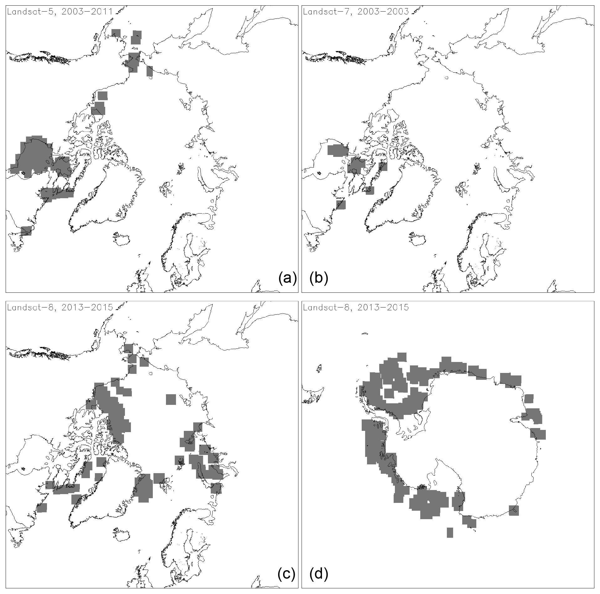
Figure 1Location of the Landsat scenes used. Panels (a–c) Arctic; panel (d) Antarctic. Note that scenes do overlap. The total number of scenes shown is 134 (a), 12 (b), 88 (c), and 134 (d).
2.2.3 Sensitivity analysis
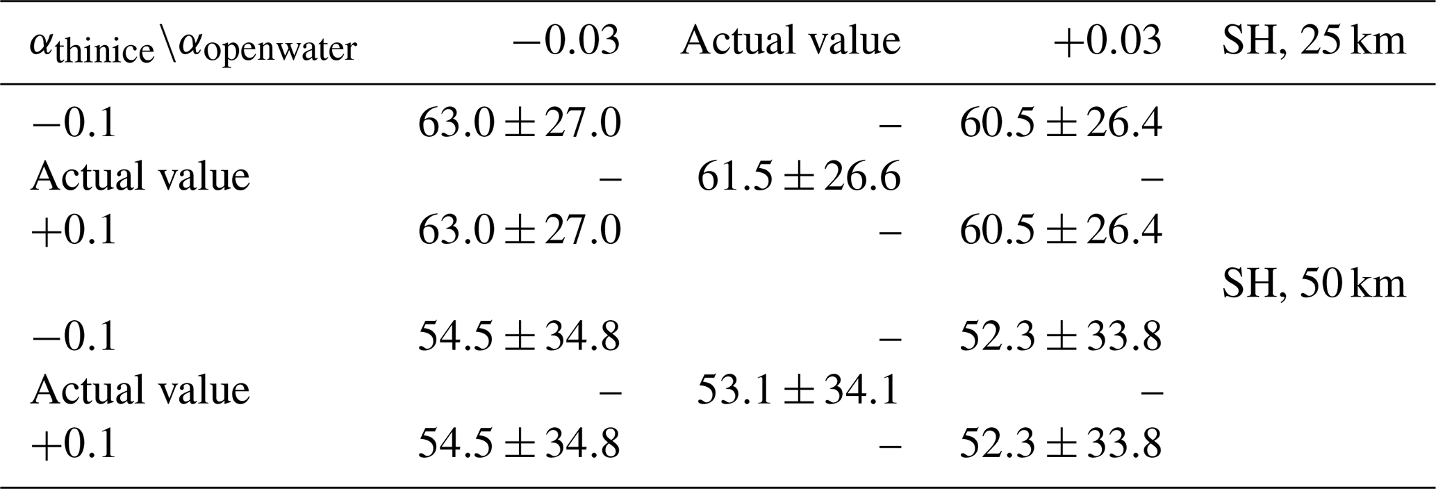
In order to estimate how Landsat SIC depends on the choice of the albedo thresholds used to discriminate open water from ice and bare/thin ice from thick/snow-covered ice, we repeat the classification into the three surface classes using modified thresholds. We vary the albedo value for the open water–ice discrimination by ±0.03; i.e., for an actual albedo value of 0.06 we employ additional threshold values of 0.03 and 0.09. We vary the albedo value for the bare/thin ice–thick/snow-covered ice discrimination by ±0.1; i.e., for an actual albedo value of 0.45 we employ additional threshold values of 0.35 and 0.55. The range of albedo threshold values we choose is motivated by our experience with the supervised classification of the many Landsat scenes under varying illumination conditions. We randomly select 12 Landsat 8 scenes for the Northern Hemisphere and 15 scenes for the Southern Hemisphere. For every image we perform the classification into the three surface classes with the above-mentioned four additional albedo threshold value combinations, compute Landsat SIC on the 25 and 50 km EASE grid, and derive a Landsat scene mean SIC value (Tables 3 and 4). We find that changing the albedo value of the open water–ice discrimination by ±0.03 changes the average Landsat SIC by between 0.7 % and 1.2 % in the Northern Hemisphere and by between 0.8 % and 1.5 % in the Southern Hemisphere. Thus, the sensitivity appears to be independent of the overall SIC which is close to 100 % for the Northern Hemisphere cases (Table 3) but 55 %–60 % for the Southern Hemisphere cases (Table 4). The difference in the sensitivity between grid resolutions of 25 and 50 km is less than 0.2 %.
Table 3Landsat SIC derived using the actual pair of albedo threshold values (“Actual value”) and the four variations of them (see text) averaged for 12 Landsat-8 scenes selected for the Northern Hemisphere (NH) at 25 and 50 km grid resolution. The number to the right of the ± denotes 1 standard deviation. All SIC values are in percent.
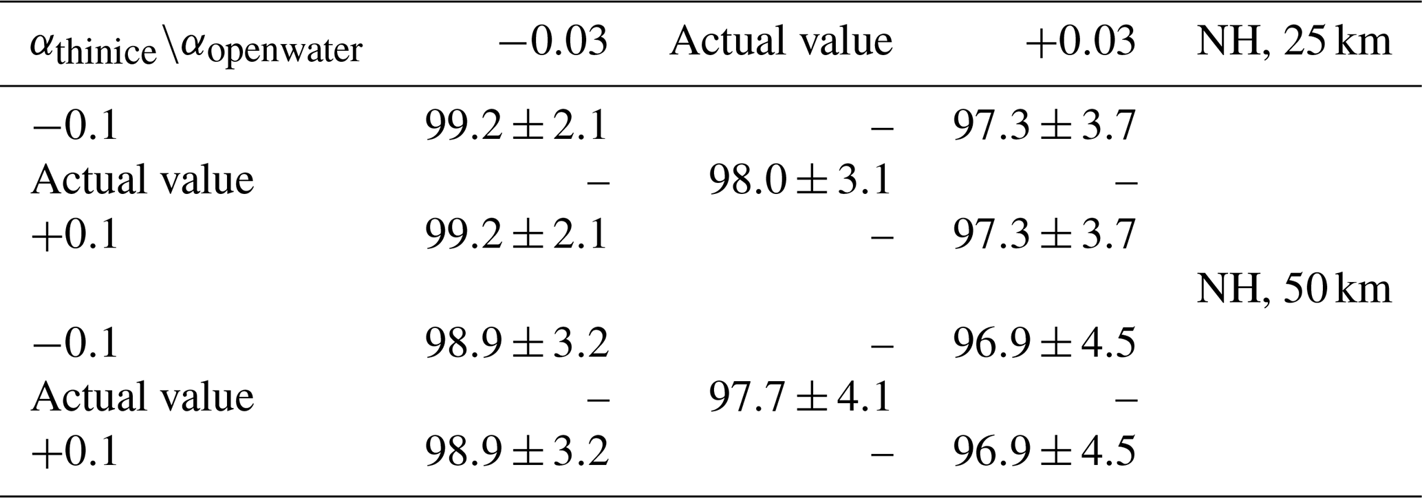
Table 4Landsat SIC derived using the actual pair of albedo threshold values (“Actual value”) and the four variations of them (see text) averaged for 15 Landsat-8 scenes selected for the Southern Hemisphere (SH) at 25 and 50 km grid resolution. The number to the right of the ± denotes 1 standard deviation. All SIC values are in percent.
As expected, changing the albedo value of the bare/thin ice–thick/snow-covered ice discrimination by ±0.1 does not influence the Landsat SIC. However, it influences the Landsat SIC computed at the respective grid resolutions when using Landsat pixels classified as thick/snow-covered ice only (Tables S2 and S3 in the Supplement). We find Landsat SIC of thick ice to vary by between 1.4 % and 2.4 % in the Northern Hemisphere and by between 2.1 % and 2.7 % in the Southern Hemisphere with little difference between the grid resolutions.
2.2.4 Potential biases in Landsat SIC
In our approach, we assume either ice or water to cover a Landsat pixel (30 m×30 m) entirely, not taking into account that ice floes or leads/openings might be smaller than the pixel size, resulting in a mixed ocean–ice pixel. This can introduce a positive bias in the Landsat SIC computed at the grid resolution of the PMW SIC products. For instance, for a Landsat pixel covered just half by thick/snow-covered sea ice, which exhibits a surface albedo of 0.8 under cold conditions, the resulting pixel average albedo would be . With that, such a pixel is classified as bare/thin ice and counts as a pixel with 100 % instead of 50 % sea-ice concentration. Depending on the albedo of the ice, an ice-cover fraction of 0.04 in one Landsat pixel could be sufficient to increase the pixel average albedo above the upper open water–ice discrimination threshold value of 0.09 (see Tables 3 and 4), causing the respective pixel to be classified as 100 % ice.
In order to quantify this positive bias better, it is useful to distinguish between sea-ice conditions during summer and winter and between pack ice and the MIZ, as well as to take into account the dimensions of leads/openings and ice floes. Distributions of lead width and floe size both follow a power law. Leads/openings and ice floes with dimensions smaller than the Landsat pixel size are orders of magnitude more abundant than wide leads/openings (e.g., Tschudi et al., 2002; Marcq and Weiss, 2012) and large ice floes (e.g., Steer et al., 2008; Toyota et al., 2011; Perovich and Jones, 2014).
Based on airborne digital camera visible imagery captured along tracks of Operation Icebridge (OIB) flights several thousands' of kilometers long in the Arctic in April 2010 and in the Antarctic in October 2009 analyzed by Onana et al. (2013) with respect to the lead and open water fraction, we find a SIC bias of less than 0.2 %. This value derived for an open water fraction of ∼1 % falls into the uncertainty range of our approach (see Tables 3 and 4) and represents winter conditions in the pack ice. Based on manual visual analysis of airborne visible imagery obtained in the MIZ in the Greenland Sea in March 1997, we find a SIC bias of the order of 5 % to 10 %. This value is clearly outside the uncertainty range of our approach. The images used here represent an ice cover of ∼70 % SIC comprising closely packed but also broken bands of a few thicker ice floes, pancake ice, and brash and grease ice with little or no new ice formation in the openings – a typical situation at an ice edge located in comparably warm water.
Next, we again take the results of Onana et al. (2013) but assume that the thin ice identified in the OIB digital camera imagery adds to the open water fraction thereby simulating a summer situation. For an open water fraction of then ∼5 %, we estimate a SIC bias of less than 0.8 %, which is still within the uncertainty range of our approach. However, this low positive bias during summer would only apply to a situation where ice floes are still packed closely together, e.g., by herding of ice floes (e.g., Toyota et al., 2016), and where gaps between the ice floes from additional openings created by the melt process are filled by brash ice and/or slush. While this is a situation that might be encountered during summer (Steer et al., 2008; Lu et al., 2008), it is not necessarily typical. In summer, it can be more common to encounter isolated floes. Depending on the size of the floes and their distribution across a 25 km grid cell with, e.g., 50 % SIC, we find the bias to range between less than 2 % to 50 % in the two most extreme cases. We refer to the Supplement to this subsection, where we describe in more detail how we obtain estimates of the positive bias caused by the combination of the finite resolution of the Landsat sensor and our classification approach for both winter and summer conditions at the scale of a 25 km PMW SIC product grid.
According to the high-resolution optical images used to infer the floe size distribution (Steer et al., 2008; Toyota et al., 2011, 2016) and similar studies (e.g., Paget et al., 2001; Lu et al., 2008; Zhang and Skjetne, 2015), the ice cover often comprises a large spectrum of floes. The larger and largest floes at the upper end of the floe-size distribution form the major fraction of the sea-ice area (in square kilometers) (e.g., Paget et al., 2001; Steer et al., 2008). A small number of large floes results in a smaller number of mixed ocean–ice Landsat pixels than a large number of smaller floes. Hence, where larger floes dominate, our Landsat SIC estimate is less biased than where small floes dominate. The effect of the ocean swell, the dominating force for fracturing ice floes according to, e.g., Toyota et al. (2016), is larger close to the ice edge than further inside the ice pack. Therefore, a larger number of smaller floes exists along the ice edge, suggesting a larger bias in our Landsat SIC near the ice edge than inside the ice pack. Without further independent information about the actual ice cover, we are not able to quantify this bias accurately.
Thus, for high-concentration winter conditions and for those cases during summer when ice floes are closely packed and openings between the floes are covered with brash ice and slush, the bias in Landsat SIC derived at the spatial scale of the PMW SIC products falls within the retrieval uncertainty range of our approach (see Tables 3 and 4). The bias could fall outside the uncertainty range near the ice edge during winter when sea ice drifts into comparably warm waters that inhibit ice formation in newly created openings; here biases as high as 10 % in a single PMW grid cell could occur. The bias could also fall outside the uncertainty range during summer; here biases between 5 % and 20 % in single PMW grid cells might occur depending on proximity to the ice edge and hence floe-size distribution and depending on conditions favoring/inhibiting herding of ice floes into bands.
In the following, we present and discuss results obtained in the Northern Hemisphere and Southern Hemisphere. We preferred to not merge the results of Landsat-5 and Landsat-8 in the Northern Hemisphere because with that we have a relatively natural discrimination between cases dominated by first-year ice (Landsat-5) and cases dominated by mixed first-year–multiyear ice or multiyear ice (Landsat-8) (see Fig. 1).
3.1 Northern Hemisphere
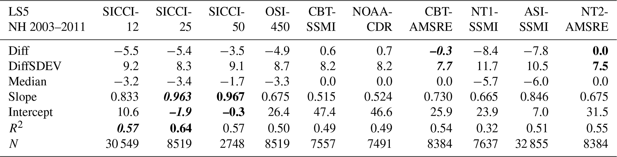
Out of the 10 products, SICCI-25km, SICCI-50km, ASI-SSMI, and SICCI-12km offer the best linear agreement with Landsat SIC for first-year-ice-dominated cases as expressed, e.g., by the location of mean and median PMW SIC (red symbols) in Fig. 2 and the values of slope, intercept, and correlation coefficient listed in Table 5. CBT-SSMI, CBT-AMSRE, NOAA-CDR, and NT2-AMSRE have the smallest overall mean difference and zero median (Table 5). These four products exhibit, however, a considerable tail of near-100 % PMW SIC values stretching across almost the entire Landsat SIC range, pointing towards overestimation of Landsat SIC. ASI-SSMI and NT1-SSMI SIC exhibit the overall largest underestimation of Landsat SIC among the 10 products (Table 5).
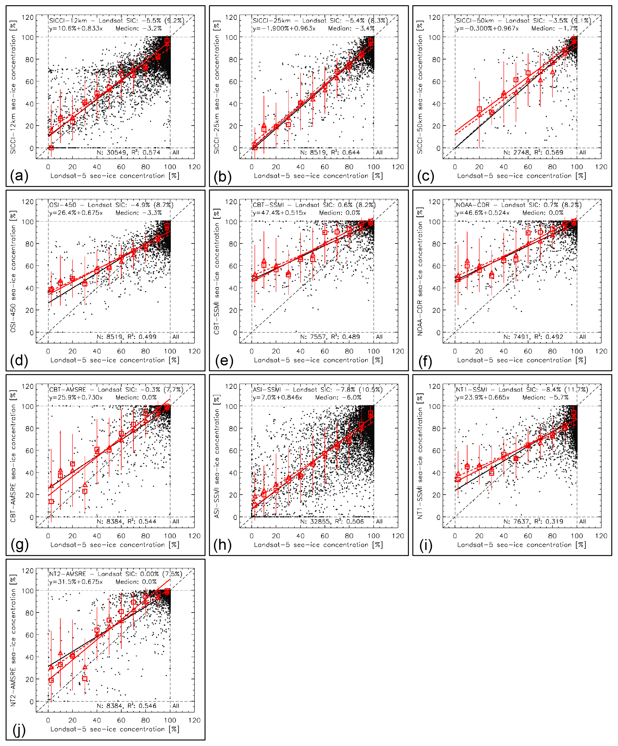
Figure 2Scatterplots of PMW SIC (y axis) versus Landsat SIC (x axis) for all 10 products for the first-year-ice-dominated cases from 2003–2011 in the Northern Hemisphere (Landsat-5). Black dots are individual data pairs, the solid black line is the linear regression, and the dashed black line is the identity line. Red triangles denote the mean PMW SIC computed for Landsat SIC ranges 0 %–5 %, 5 %–15 %, 15 %–25 %, …, 85 %–95 %, 95 %–100 %, red bars denote 1 standard deviation of these mean values, and the dashed red line is the respective linear regression line. Red squares denote the median PMW SIC for the same Landsat SIC ranges, and the solid red line is the respective linear regression line. The overall mean and median difference PMW SIC minus Landsat SIC, its standard deviation, and the equation of the linear regression through the individual data pairs are shown at the top and the number N of data pairs and the squared linear correlation coefficient at the bottom of each panel.
Table 5Summary of the statistical parameters displayed in Fig. 2. Diff, DiffSDEV, and Median (all in percent SIC) are the mean difference PMW SIC minus Landsat (LS) SIC, its standard deviation, and the median difference, Slope and Intercept (in percent SIC) are the coefficients of the linear regression, and R2 and N are the squared linear correlation coefficient and number of data pairs, respectively. Numbers in bold and bold italic font denote the respective “best” and “second best” value, respectively, e.g., largest and second largest values of R2 and lowest and second lowest values of Diff, Intercept, and the difference of unity minus slope.
For cases with mixed first-year–multiyear or multiyear ice, SICCI-25km and SICCI-50km offer best linear agreement with Landsat SIC (Fig. 3). Most other products have a less convincing linear relationship. Like for first-year ice, CBT-SSMI, CBT-AMSR2, NOAA-CDR, and NT2-AMSR2 have the smallest mean difference for mixed first-year–multiyear or multiyear ice (Fig. 3, Table 6). However, particularly at higher Landsat SIC these products show many data pairs above the identity line, and the linear regressions through the mean and median PMW SIC (dashed and solid red lines) are also located above the identity line – in contrast to, e.g., SICCI-25km and SICCI-50km.
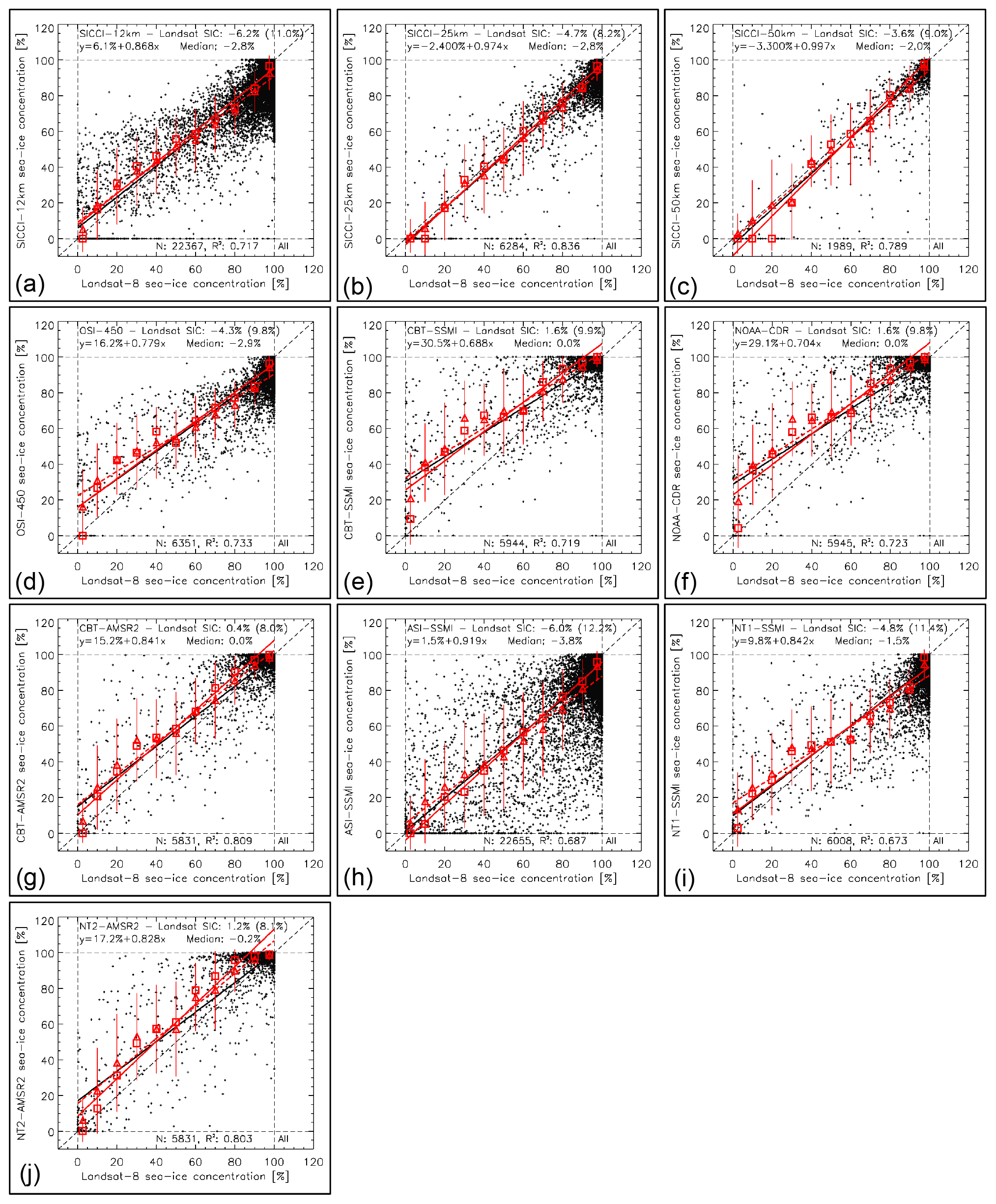
Figure 3Scatterplots of PMW SIC (y axis) versus Landsat SIC (x axis) for all 10 products for mixed first-year–multiyear or multiyear ice cases from 2013 to 2015 in the Northern Hemisphere (Landsat-8). See Fig. 2 for a description of symbols, lines, and text.
Table 6Summary of statistical parameters shown in Fig. 3. See Table 5 for an explanation of the parameters given.
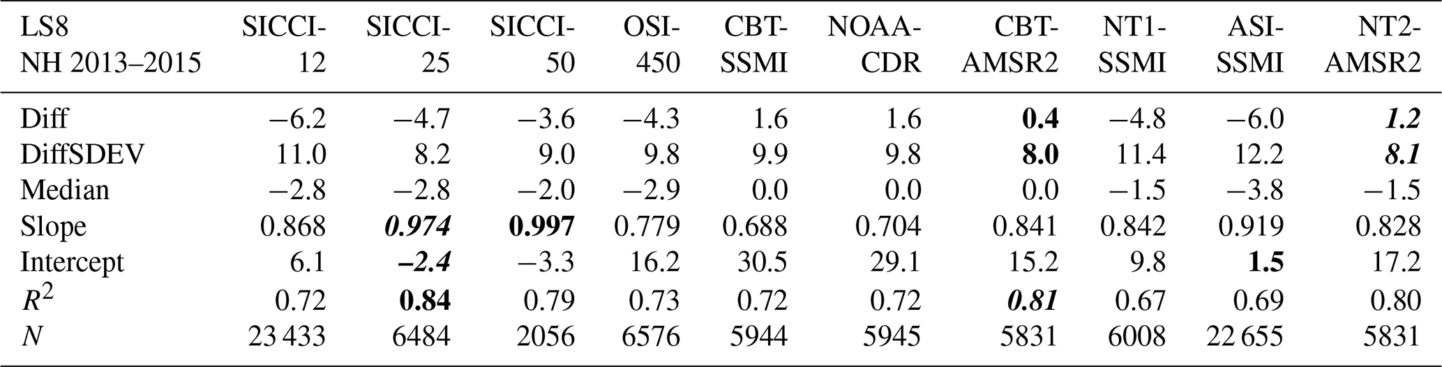
The linear agreement between PMW SIC and Landsat SIC improves in general for all 10 products for mixed first-year–multiyear or multiyear ice cases (Fig. 3, Table 6) compared to first-year ice (Fig. 2, Table 5). This improvement is comparably large for OSI-450 (slope increases by ∼0.10) and NT2-AMSR (slope increases by ∼0.15) but quite small for SICCI-25km and SICCI-50km because slopes are close to unity already. Hence, despite the larger magnitude of overall mean and median SIC differences, of all 10 products SICCI-25km and SICCI-50km provide SIC estimates for first-year ice that are almost as accurate as those for mixed first-year–multiyear ice or multiyear ice. This could be one consequence of the self-optimizing hybrid SICCI-2 and OSI-450 algorithm (Lavergne et al., 2019) and of the way ice tie points are chosen in comparison to the other products (e.g., Kern et al., 2020b).
3.2 Southern Hemisphere
In the Southern Hemisphere, slope and location of the linear regression lines, as well as of the mean and median PMW SIC values (red symbols), are more similar between the 10 products (Fig. 4, Table 7). The linear agreement is fairly good for SICCI-2 products, CBT-AMSR2, and ASI-SSMI. Like in the Northern Hemisphere, SICCI-25km and SICCI-50km reveal the best linear agreement with Landsat SIC, but SICCI-50km appears to be negatively biased. This bias is associated with a large number of PMW SIC values of 0 % at non-zero Landsat SIC which is also reflected by the mean and median PMW SIC (compare Fig. 4c with Fig. 3c). We discuss this issue and the observation that all products except CBT-SSMI, NOAA-CDR, and CBT-AMSR2 exhibit SIC values below about 10 %–15 %, while these three products lack values in the PMW SIC range between 0 % and ∼15 % in Sect. 5.3.
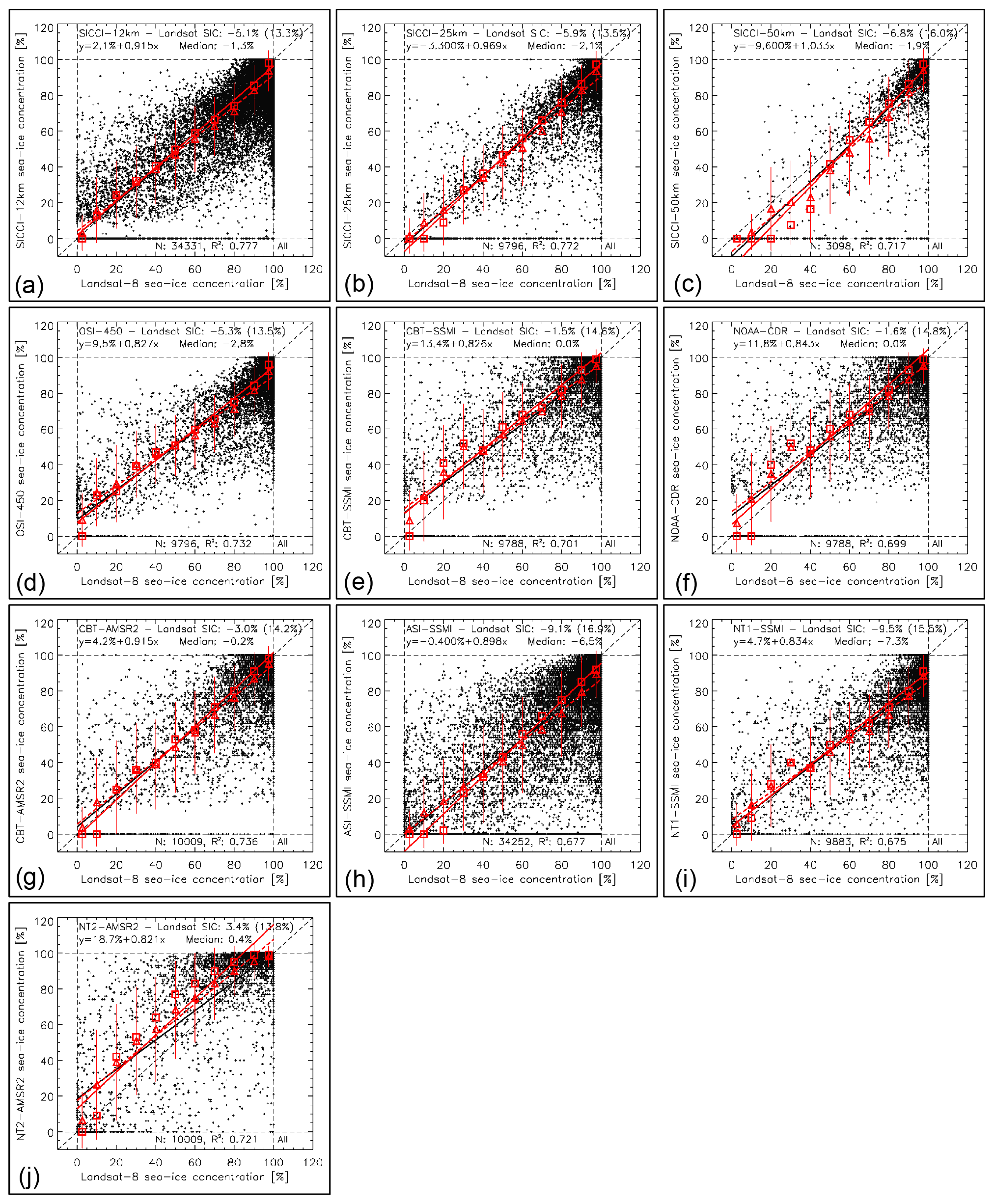
Figure 4Scatterplots of PMW SIC (y axis) versus Landsat SIC (x axis) for all 10 products for 2013–2015 in the Southern Hemisphere. See Fig. 2 for a description of symbols, lines, and text.
Table 7Summary of statistical parameters shown in Fig. 4. See Table 5 for an explanation of the parameters given.
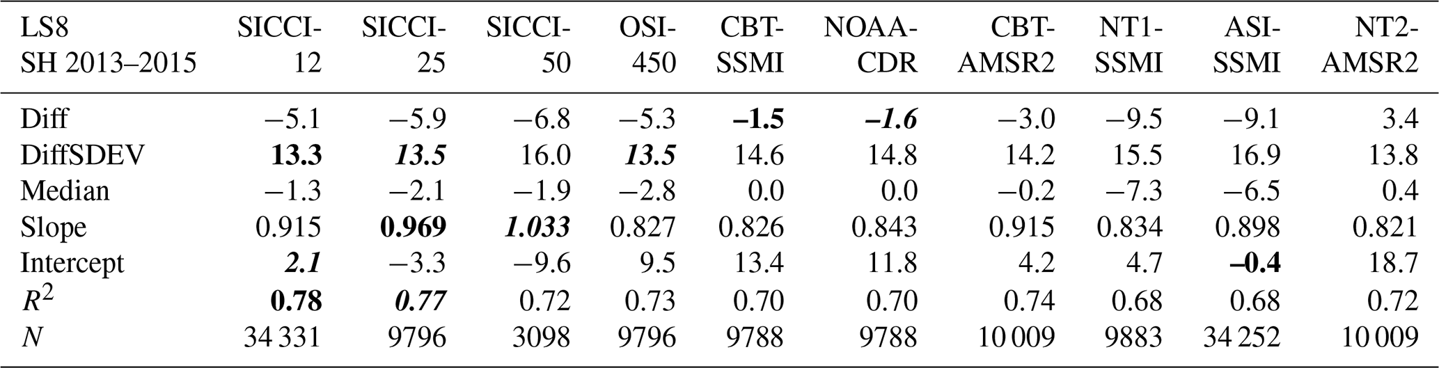
Like in the Northern Hemisphere (Table 6), the magnitude of the SIC difference is smallest for NT2-AMSR2, NOAA-CDR, CBT-SSMI, and CBT-AMSR2 and largest for NT1-SSMI and ASI-SSMI. Of all 10 products, NT2-AMSR2 (Fig. 4j) offers the most asymmetric SIC distribution and a considerable overestimation of Landsat SIC in the range between ∼40 % and ∼90 %, also expressed by median SIC > mean SIC for all Landsat SIC bins above 25 % (Fig. 4j). NT2-AMSR2 is the only product with a substantial positive overall mean difference of 3.4 %; even the median difference is >0 % (Table 7).
3.3 Hemispheric similarities and differences
Overall, agreement between PMW SIC and Landsat SIC differs between the two hemispheres. For all products, we find a substantially larger scatter of SIC values around the identity line in the Southern Hemisphere (Sect. 3.2) than the Northern Hemisphere (Sect. 3.1). On the one hand, this larger scatter in the Southern Hemisphere could be the result of a considerably larger number of Landsat scenes of cases with low SIC, naturally resulting in a larger spread of the SIC. In addition, the majority of the Landsat scenes in the Southern Hemisphere reflect late-spring/summer conditions. During such conditions, snow metamorphism due to melt and melt–refreeze cycles substantially change the sea-ice surface emissivity on daily timescales and sub-grid-cell-size spatial scales (e.g., Willmes et al., 2014), causing a larger scatter in SIC. Another factor impacting the sea-ice emissivity is flooding at the interface between the sea ice and the snow cover formation, causing considerable variations in basal snow layer wetness and salinity on similar spatiotemporal scales. On the other hand, we are dealing with an unknown amount of overestimation of the actual sea-ice concentration by our Landsat SIC during summer melt due to mixed ocean–ice Landsat pixels (Sect. 2.2.4). We refer to Sects. 4.3, 5.1 and 5.2 for more discussion on this issue.
In general, we find the scatter is larger for products with finer grid resolution, e.g., SICCI-12km and ASI-SSMI, than for the coarser-grid-resolution products. The larger number of valid SIC pairs of the high-resolution products result in more scatter due to the inherent retrieval noise even though the capability to resolve smaller-scale SIC variations is better for the fine-resolution than for the coarser-resolution products (see Sect. 5.1). In addition, a mismatch in the location of, for example, a 10 km scale patch of ice between a Landsat scene and a PMW SIC product has a substantially larger influence on the SIC difference at 12.5 than at 25 or 50 km grid resolution. The fact that oversampling is much larger at 12.5 than at 50 km plays a role here also. Even using simulated brightness temperatures one gets a large spread between a reference SIC and the PMW SIC due to resolution mismatch (see, e.g., Tonboe et al., 2016). We discuss the effect of different footprint sizes and grid resolutions (see Table 1) in more detail in Sect. 5.1.
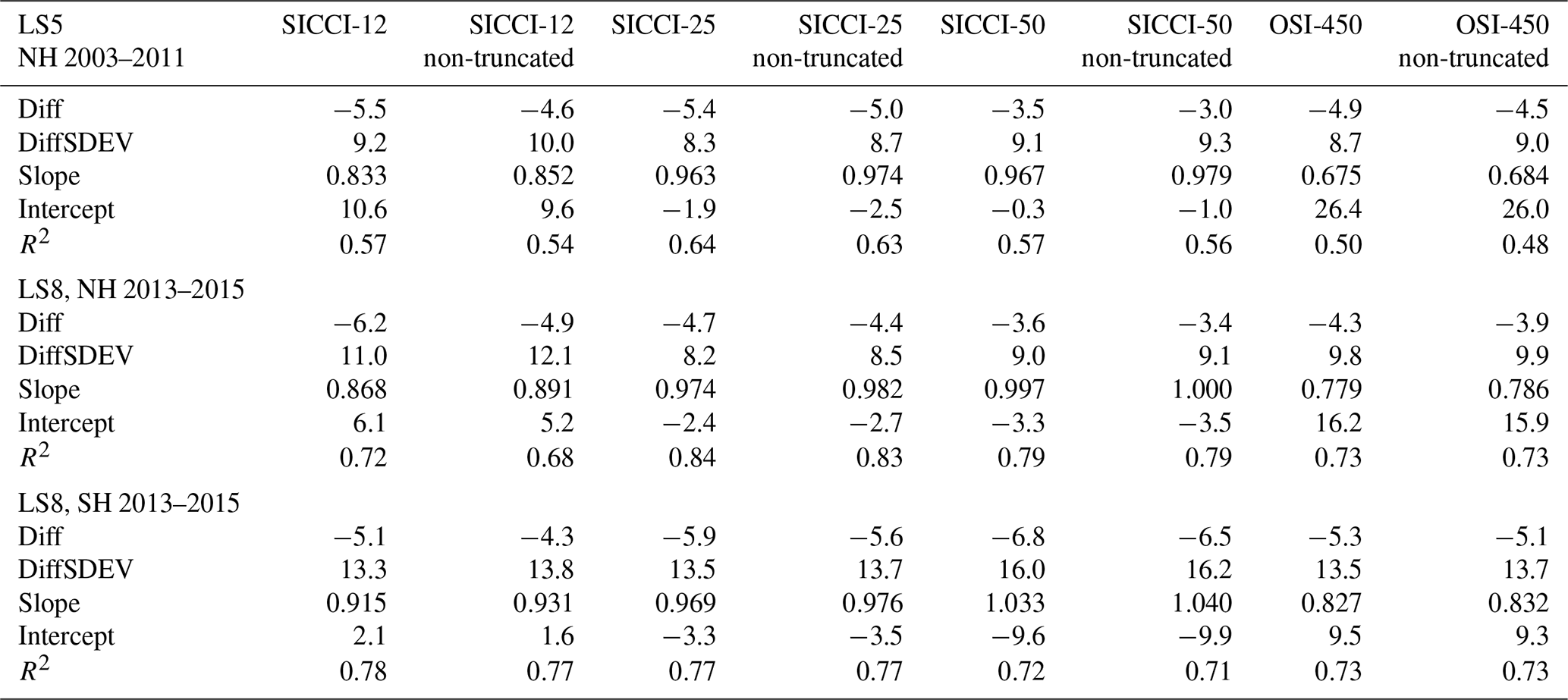
SICCI-2 products and OSI-450 provide access to SIC values above 100 % and below 0 % that are naturally retrieved due to the brightness temperature distribution around the ice and water tie points used. Kern et al. (2019) found that incorporation of these so-called off-range or non-truncated SIC values provides a more accurate estimate of accuracy, i.e., difference to the true SIC value, and precision, i.e., standard deviation of this difference. Table 8 reveals that independent of the ice type, the magnitude of the mean difference decreases, while the slope of the linear regression increases, becoming closer to unity in most cases, in agreement with Kern et al. (2019). Of particular interest in this regard are high-concentration cases discussed in more detail in Sect. 4.2 but also the effect of the truncation at 0 % in the context of filters used to mitigate spurious SIC values (see Sect. 5.3).
Table 8Comparison of statistical parameters listed in Tables 5–7 in both hemispheres for SICCI-2 and OSI-450 products using truncated or non-truncated (near-100 % SIC) PMW SIC data. See Table 5 for an explanation of the parameters given. Top (LS5, NH 2003–2011) is for first-year-ice-dominated cases, middle (LS8, NH 2013–2015) is for mixed first-year–multiyear and multiyear ice cases, both Northern Hemisphere, and bottom (LS8, SH 2013–2015) is for the Southern Hemisphere. The overall median differences do not change and are not listed again.
In the previous section, we showed results independent of the ice regime (see below) – except for a general discussion of the observed differences between predominantly first-year ice (Landsat-5) and a mixture of first-year–multiyear or multiyear ice (Landsat-8). This section deals with our comparison between PMW SIC and Landsat SIC for the following ice regimes: “ice edge”, “leads and openings” meaning cases with leads and coastal polynyas or openings, “heterogeneous ice” meaning cases with irregularly shaped openings in the ice pack, “freeze-up”, “high-concentration ice”, and “melt conditions” (see Table S1 in the Supplement). We show in more detail results of the last three ice regimes. Freeze-up cases are characterized by a comparably large fraction of new and thin ice, an ice type for which some of the SIC products investigated here are already known to be negatively biased from preliminary work based on Soil Moisture and Ocean Salinity (SMOS) thin ice thickness observations (Ivanova et al., 2015). We elaborate on their findings using an alternative data set. Investigating high-concentration cases in more detail aids in a better understanding of saturation effects near 100 % caused by truncating PMW SIC at 100 %, expanding on the work of Kern et al. (2019) and refining our knowledge of SIC precision and accuracy for high-concentration regions and hence application potential of the products for surface heat flux computations. Finally, melt conditions – even without melt ponds – represent a multitude of different snow and sea-ice conditions causing enhanced variability in the sea-ice microwave emissivity (e.g., Willmes et al., 2014), which in turn can result in biases in PMW SIC products of both signs in the Arctic (Kern et al., 2016, 2020b). Here we have the opportunity to better quantify such biases especially for the Antarctic. For all remaining regimes, we show examples in Figs. S3–S8 in the Supplement and include their results of the statistical comparison into our summary figures (Figs. 11 and 12) but refrain from a detailed discussion. For regimes “ice edge” and “leads and openings” such a discussion would require a comprehensive investigation of open water and land spillover filters (see Sect. 5.3) which is beyond the scope of this paper. For regime “heterogeneous ice”, application of a more accurate evaluation SIC data set seems to be advisable given the identified shortcomings of the one used (see Sect. 2.2.4) before going into more detail.
4.1 Freeze-up
These are cases when according to the date, geographic location, and information in the Landsat scene freeze-up has commenced. We select Landsat scenes containing a considerable fraction of new and thin ice; these are acquired in September and February/March in the Northern Hemisphere and Southern Hemisphere, respectively. We have only a few such cases in both hemispheres (see Table S1). We expect PMW SIC underestimates Landsat SIC (LSIC) – particularly for young and thin ice with a thickness <0.2 m (e.g., Ivanova et al., 2015). Figure 5 illustrates the conditions for a Landsat-8 scene close to Greenland in the Fram Strait on 15 September 2015. The classified Landsat-8 image (Fig. 5, top left) reveals a mix of large ice floes – presumably second-year or older ice – and meandering patches of smaller floes embedded into a matrix of mostly gray and a few dark pixels; the gray pixels are supposed to represent bare/thin sea ice and the dark pixels open water. All products agree well with Landsat SIC in the topmost part of the scene over high-concentration ice. PMW SIC maps of 6 of the 10 products (SICCI-2 products, OSI-450, NT1-SSMI, and ASI-SSMI) reveal an overall SIC distribution similar to Landsat SIC. For the remaining four products, the SIC difference maps show widespread overestimation of LSIC by PMW SIC expressed by positive (red) values. Contrary to expectations, we do not observe negative SIC differences for the entire greyish area of the Landsat-8 scene.
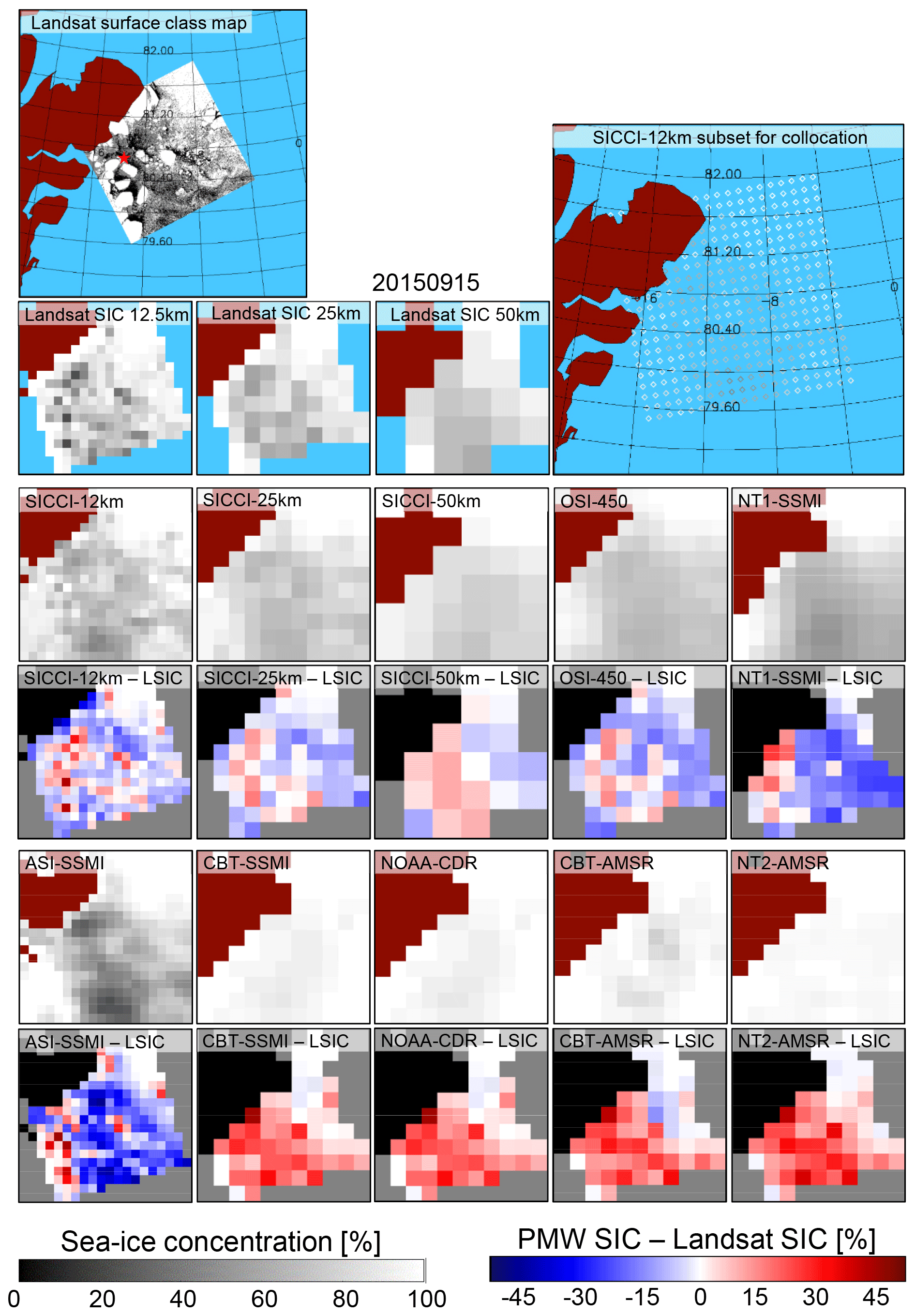
Figure 5Landsat SIC, PMW SIC, and the difference PMW SIC minus Landsat SIC (LSIC) for all 10 products for a freeze-up case in the Fram Strait on 15 September 2015. The Landsat surface class map at the top left shows the following: white: thick/snow-covered ice; gray: bare/thin ice; black: open water. The red star marks the location of Henrik Krøyer Holme station (see text). White and gray pixels are used to compute maps of gridded LSIC at 12.5, 25, and 50 km, respectively (blue: outside Landsat image). A subset of SICCI-12km SIC grid cells shown at the top right illustrates the array used for the collocation. Panels in the remaining four rows show PMW SIC and PMW SIC minus LSIC for all 10 products. Land is flagged brown in the SIC panels and black in the SIC difference panels; it differs between the PMW products. The land masks in the two bigger maps at the top come from the plotting routine used. LSIC maps use the land masks of the SICCI-2 products.
The main reason for this observation is the actual ice condition. Very likely the greyish area represents a mixture of sub-pixel-size, i.e., less than 30 m×30 m, ice floes and brash ice formed from disintegrated thicker ice floes and young/new sea ice. On the one hand, the sub-pixel-size floes and the brash ice are thicker than young/new sea ice. These forms of sea ice exhibit different surface properties and hence microwave emissivity than young/new thin sea ice. For such a mixture of ice types, it is particularly difficult to retrieve an accurate SIC with any of the algorithms used in the 10 products. Ice tie points do not adequately represent these ice conditions. On the other hand, for the greyish area the Landsat SIC could likely be too high because of mixed ocean–ice Landsat pixels (see Sect. 2.2.4 and the respective Supplement section). What appears to be 100 % thin ice might be just 50 % thick ice. However, observations conducted at Henrik Krøyer Holme station ( N, W; see star in Fig. 5, top left panel) on 15 September 2015 and the preceding days indicate freezing conditions with air temperatures between −5 and −13 ∘C (https://www.dmi.dk, last access: 29 June 2021). Therefore, it is quite likely, new/thin ice covers most open water patches, and any overestimation of Landsat SIC due to sub-pixel-size open water patches is rather small. Thus, the complex sea-ice conditions encountered appear to be a valid explanation for the observed differences. Contributing factors are also the different footprint sizes and grid resolutions that cause heterogeneous sub-grid surface conditions to be mixed differently (see the panels for the three SICCI products in Fig. 5) and an unaccounted weather influence. An apparent underestimation of the SIC (see, e.g., ASI-SSMI) could be caused by actual weather conditions being less severe, i.e., smaller atmospheric water vapor content, than are included inherently in the open water tie point used (see also Kaleschke et al., 2001).
Figure 6 illustrates a freeze-up case in Pine Island Bay, Amundsen Sea, Southern Ocean, on 12 March 2014. The classified Landsat-8 scene features a predominant coverage with new/young ice, some open water towards the coast, and little thick/snow-covered ice and few icebergs in the open bay. Landsat SIC is mostly around 90 %; only a few grid cells with low SIC exist close to the coast at 12.5 and 25 km grid resolution. A total of 9 of the 10 PMW SIC products reveal considerably lower SIC values, with SICCI-25km, OSI-450, NT1-SSMI, and ASI-SSMI exhibiting particularly large widespread negative differences with magnitude >40 %. An exception is NT2-AMSR2 exhibiting the highest PMW SIC of all 10 products and overall the smallest differences. It is the only product, though, which also exhibits positive differences, i.e., an overestimation of Landsat SIC by up to 20 %.

Figure 6Landsat SIC, PMW SIC, and the difference PMW SIC minus Landsat SIC for all 10 products for a scene near the coast during freeze-up in Pine Island Bay, Amundsen Sea, Southern Ocean, on 12 March 2014. The red star in the top left map marks the location of the Pine Island Glacier Automatic Weather Station (see text). Some of the white patches near the coast in this map are actually glacier ice not adequately flagged by the land mask. See Fig. 5 for more details.
The widespread underestimation of Landsat SIC by almost all products agrees very well with the findings of Ivanova et al. (2015), albeit a bit large in magnitude. The new ice encountered in our example comprises a comparably large fraction of frazil, grease, and/or small pancake ice compared to nilas and gray/gray-white ice in Ivanova et al. (2015). Because Pine Island Glacier Automatic Weather Station (see star in top left map of Fig. 6) reported air temperatures between −11 and −21 ∘C on 12 March 2014 and the 3 preceding days (Mojica Moncada et al., 2019), the gray pixels in this Landsat scene very likely represent new/thin sea ice formed locally. However, we cannot fully exclude an overestimation of Landsat SIC by sub-pixel-size open water patches between streaks of new ice formed being classified as thin ice instead of open water (see Sect. 2.2.4 and respective Supplement section); for the conditions encountered this positive bias in Landsat SIC should be less than 5 % and maximum 10 %. The existence of such a positive bias combined with the different ice type encountered compared to Ivanova et al. (2015) could explain why the observed underestimation of Landsat SIC for most of the PMW SIC products is larger in magnitude than expected.
Table 9 summarizes our results of the freeze-up cases for which we expect, overall, an underestimation of Landsat SIC, i.e., a negative bias, due to a notable fraction of new/thin ice (see Ivanova et al., 2015). In the Northern Hemisphere, performance of the products differs a lot. We find positive biases for CBT-SSMI, CBT-AMSR2, NOAA-CDR, and NT2-AMSR2 and large negative biases for the remaining products. SICCI-25km offers the best linear agreement with Landsat SIC. In the Southern Hemisphere, a number of products have a regression line slope close to unity, a small intercept, and a squared linear correlation coefficient >0.8. Most importantly, however, all products – except NT2-AMSR2 – on average underestimate Landsat SIC in agreement with Ivanova et al. (2015).
Table 9Summary of statistical results obtained for three freeze-up cases in the Northern Hemisphere (NH) and for 11 freeze-up cases in the Southern Hemisphere (SH) using Landsat 8 data. See Table 5 for an explanation of the parameters given.

4.2 High-concentration ice
These are cases when the Landsat scene indicates either a closed ice cover without any leads or openings or an almost closed ice cover with few refrozen leads or openings, resulting in near-100 % Landsat SIC. In the ideal case, we expect PMW SIC is close to 100 %. Figure 7 illustrates such a case for 4 April 2015 in the Beaufort Sea, Arctic Ocean. Landsat SIC is 100.0 %. All 10 PMW SIC products exhibit quite high sea-ice concentrations – particularly SICCI-50km, NOAA-CDR, and NT2-AMSR2. However, the difference maps clearly reveal a (very) small and negative bias for all PMW products. This bias is largest in magnitude for SICCI-12km and ASI-SSMI and smallest in magnitude for NT2-AMSR2.
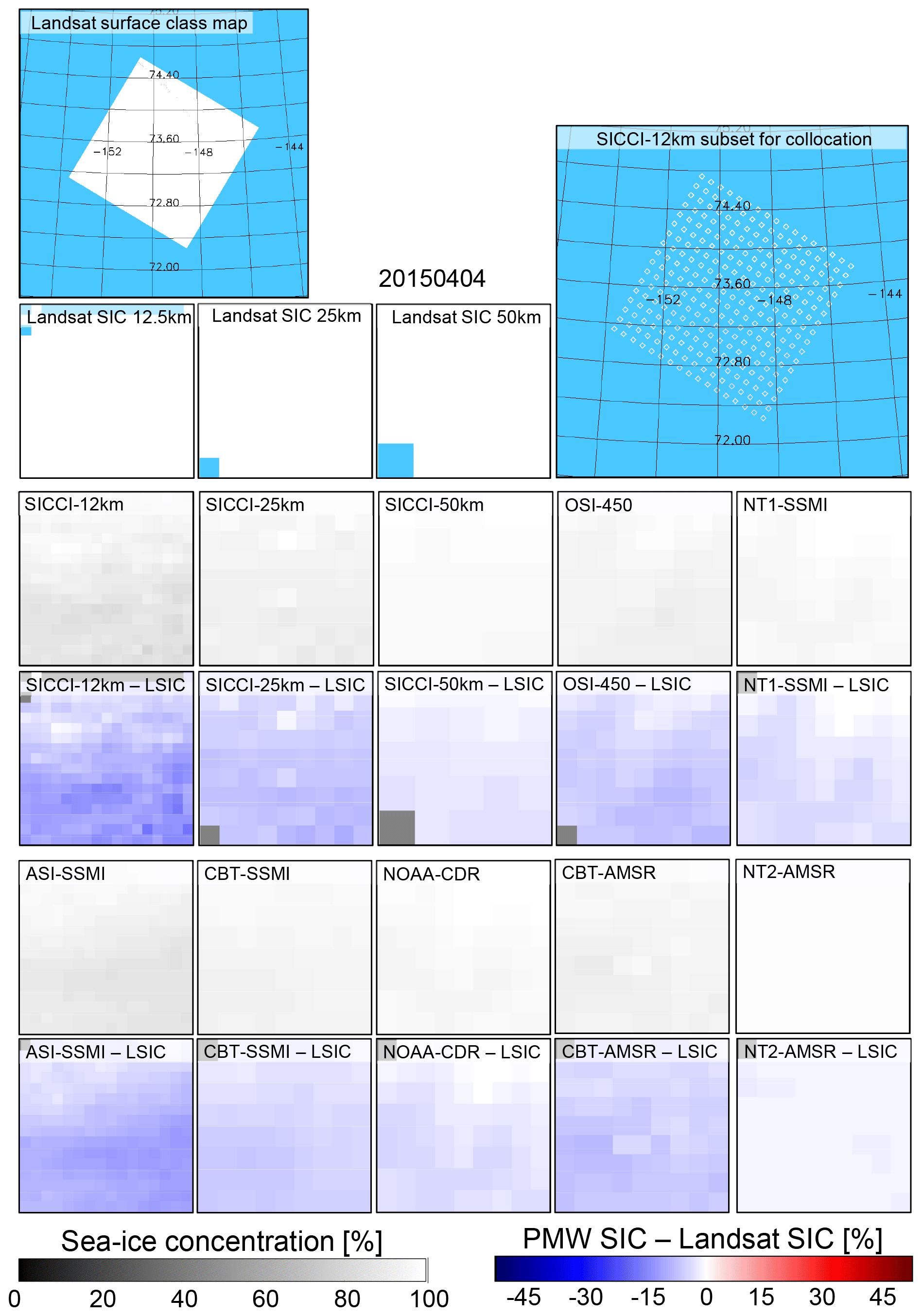
Figure 7Landsat SIC, PMW SIC, and the difference PMW SIC minus Landsat SIC for all 10 products for a high-concentration scene in the Beaufort Sea, Arctic Ocean, on 4 April 2015. See Fig. 5 for a description of the maps shown.
Table 10 summarizes the results obtained for, in total, 40 high-concentration cases in the Northern Hemisphere: 28 first-year-ice-dominated scenes (Landsat-5) and 12 scenes of mixed first-year–multiyear or multiyear ice cases (Landsat-8). We find the largest biases for SICCI-12km and ASI-SSMI independent of ice type. Except for CBT-AMSR and NT2-AMSR, all products exhibit a larger bias for first-year ice cases than mixed first-year–multiyear or multiyear ice cases. We hypothesize that the different biases between PMW and Landsat SIC for these near-100 % cases are caused by the different capabilities of the respective algorithms to derive an accurate SIC independent of ice type – as stated already in Sect. 3.1. NT1-SSMI and ASI-SSMI appear to have the largest difficulties with the different ice types encountered because their biases vary most. CBT-SSMI, CBT-AMSR, NOAA-CDR, and NT2-AMSRE have a median difference of 0.0 % independent of ice type – similar to Tables 5 and 6. For SICCI-2 products and OSI-450, median differences are smaller in magnitude than for all ice and approach zero for the mixed first-year–multiyear or multiyear ice cases.
Table 10Summary of statistical results obtained in the Northern Hemisphere for 28 cases with first-year ice (top, LS5, NH 2003–2011) and for 12 cases with mixed first-year–multiyear or multiyear ice (bottom, LS8, NH 2013–2015). See Table 5 for an explanation of the parameters shown. For SICCI-2 and OSI-450 products, we include in all rows but “N” values based on non-truncated (near 100 %) SIC data to the right of the “/”. We omit slope and intercept because SIC data pairs cluster at 100 %.
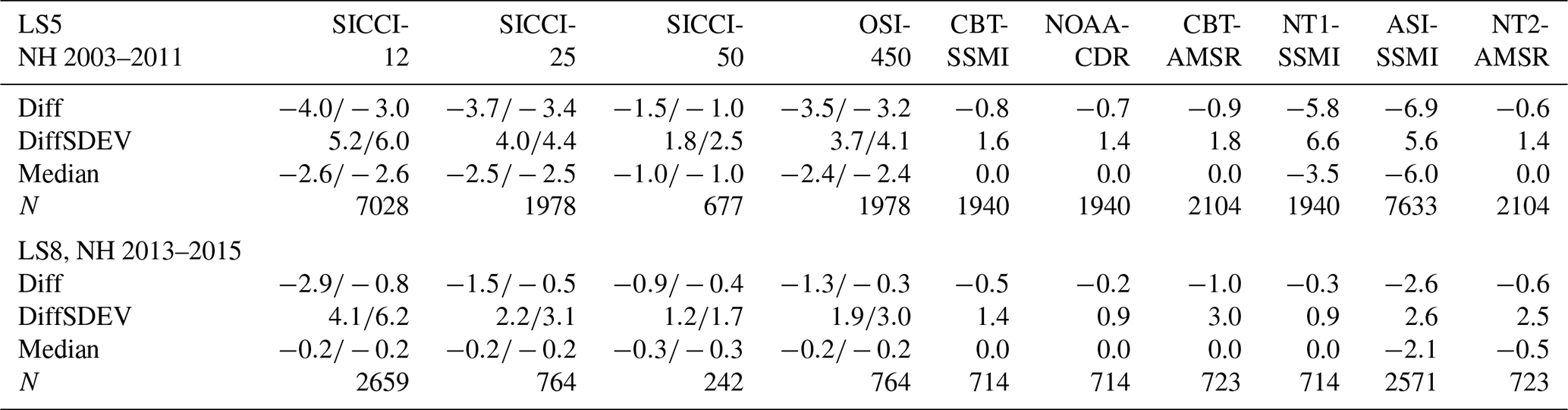
Using non-truncated SIC of SICCI-2 products and OSI-450 (see also Table 8) reduces the magnitude of the bias by between 0.5 % for SICCI-50km and 2.1 % for SICCI-12km for the mixed first-year–multiyear or multiyear ice cases (LS8) and less than that for the first-year ice cases. As expected, the standard deviation of the bias increases using non-truncated SIC. The other six PMW products set SIC values >100 % to 100 % or do not permit a simple retrieval of such SIC values (NT2-AMSR, but see Ivanova et al., 2015) and would therefore have a different bias and a larger standard deviation than shown in Table 10 (see Kern et al., 2019). Of the SICCI-2 and OSI-450 products, SICCI-50km provides the smallest bias and the smallest standard deviation of this bias: % in line with Kern et al. (2019) who reported a bias of % for non-truncated SICCI-50km SIC.
Figure 8 illustrates a high-concentration case in the Weddell Sea, Southern Ocean, on 12 March 2015. A total of 6 of the 10 PMW SIC products show almost 100 % sea-ice concentration and almost zero bias. We only find notable deviations from 100 % concomitant with a small negative bias for ASI-SSMI, CBT-SSMI, CBT-AMSR2, and SICCI-12km. For our four high-concentration cases in the Southern Ocean (Table 11), we find the largest overall bias for ASI-SSMI. Most products reveal a bias of magnitude 0.3 % or smaller.
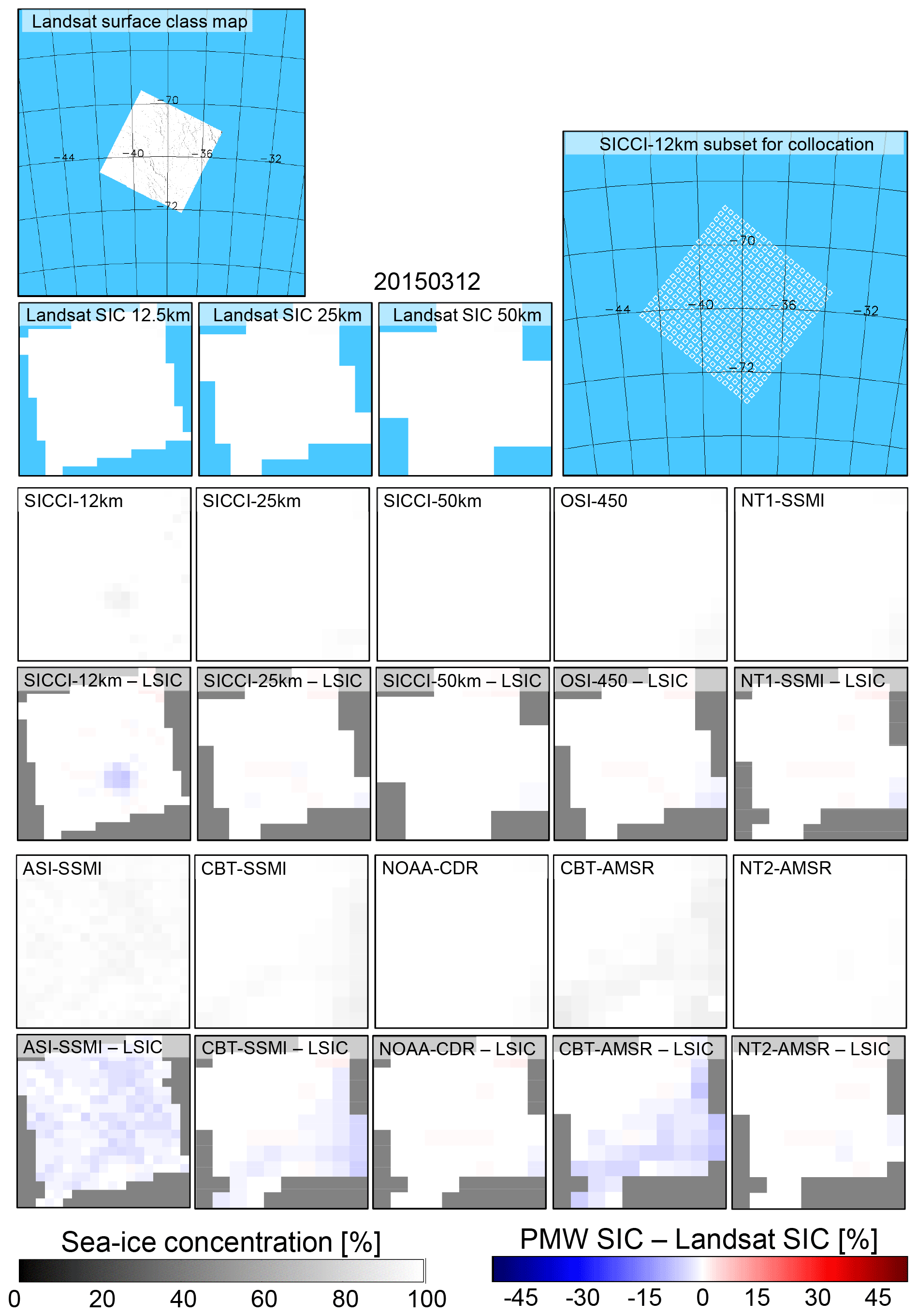
Figure 8Landsat SIC, PMW SIC, and the difference PMW SIC minus Landsat SIC for all 10 products for a high-concentration scene in the Weddell Sea, Southern Ocean, on 12 March 2015. See Fig. 5 for a description of the maps shown.
Table 11Summary of statistical results obtained for the four high-concentration cases in the Southern Hemisphere. See Table 5 for an explanation of the parameters shown. For SICCI-2 and OSI-450 products, we include in rows “Diff”, “DiffSDEV”, and “Median” values obtained using non-truncated SIC to the right of the “/”.
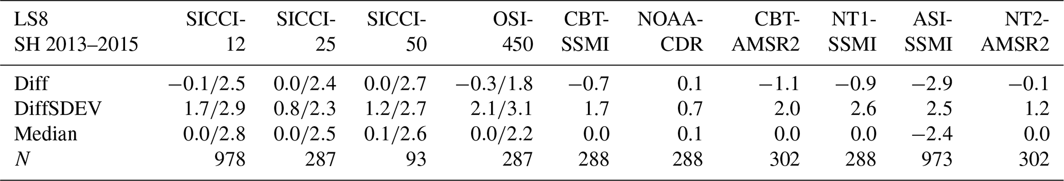
Using non-truncated SICCI-2 and OSI-450 SIC results in positive biases, ranging between 1.8 % for OSI-450 and 2.7 % for SICCI-50km (Table 11, values to the right of the “/”). This amounts to an increase in the mean SICCI-2 and OSI-450 SIC for these cases by ∼2.5 %. This increase is larger than in the Northern Hemisphere (compare Table 10). We explain this with a comparably large fraction of PMW SIC>100 % for our small high-concentration case data set of the Southern Hemisphere (4) compared to the Northern Hemisphere (40). Three of the four high-concentration cases identified in the Southern Ocean are from the months of November and December, a time of the year when melt onset and melt–refreeze cycles cause higher variability in the ice emissivity. One of the likely impacts is a notable fraction of PMW SIC>100 % (see Fig. S1 in the Supplement). The same applies in a different way to the case shown in Fig. 8, the only late-fall/early winter case out of these four cases. The overall Landsat SIC of this scene is 99.9 %; that of an adjacent scene is 98.9 % (not shown). Sea-ice and snow properties in late-fall/early winter are often quite variable as well and can cause an elevated spread of the retrieved PMW SIC around 100 %, resulting in a substantial fraction of SIC values >100 %. For instance, the overall SICCI-25km SIC is 101.9 % for the scene shown in Fig. 8 and 103.1 % for the adjacent scene (not shown).
4.3 Melt conditions
For melt-condition cases, we select Landsat scenes by means of the calendar date. In the Northern Hemisphere, we consider the time period 15 May to 31 May; in the Southern Hemisphere, we use the time period 15 November to 28 February. We do not include Landsat scenes subject to melt ponding on sea ice, e.g., during the months of June through August; this topic is covered in Kern et al. (2020b).
In the Northern Hemisphere (Table 12), we find positive and comparably small biases for CBT-SSMI, CBT-AMSR2, NOAA-CDR, and NT2-AMSR2 and negative biases for all other products. We find the best quality of the linear agreement between PMW SIC and Landsat SIC for SICCI-25km, followed by SICCI-50km and SICCI-12km. According to Kern et al. (2020b), the second half of May is characterized by an upswing in the number and magnitude of SIC values >100 % for SICCI-2 and OSI-450 products (see Fig. S2 in the Supplement). Using non-truncated SIC of these products reduces the mean bias by 1.0 % for SICCI-12km, 0.5 % for SICCI-25km, and 0.3 % for OSI-450 and further improves the already good linear agreement. For SICCI-50km, results remain almost unchanged. We explain the difference in the response between SICCI-50km and SICCI-12km by the greater sensitivity of the higher frequency channels used by SICCI-12km to early stages of melt encountered at that time of the year.
Table 12Summary of statistical results obtained for 15 melt-condition cases (without melt ponds) in the Northern Hemisphere. See Table 5 for an explanation of the parameters shown. Numbers added to the right of the “/” for SICCI-2 and OSI-450 products denote the results obtained using non-truncated SIC.
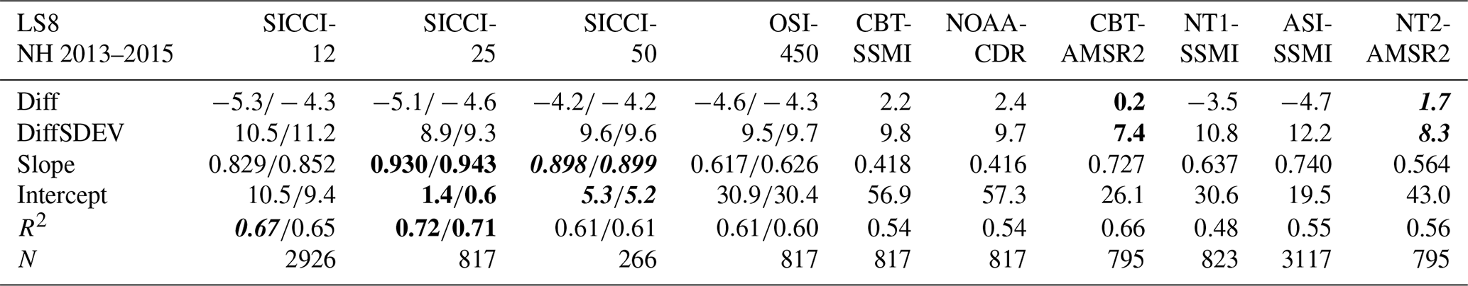
Figure 9 illustrates a typical case of late-summer melt conditions in the Ross Sea, Southern Ocean. The classified Landsat-8 image shows a heterogeneous mixture of black, gray, and white pixels. The gray pixels denote a mixture of open water and thicker ice, possibly brash ice, sea ice with a wet or even flooded snow cover, or bare relatively thick ice from which the snow has been washed off. New/young ice is unlikely according to 6 hourly forecasts of the Antarctic Mesoscale Prediction System (AMPS), revealing near-surface temperatures around −1 ∘C on 27 January 2014 and between −3 and −5 ∘C on 28 and 29 January 2014 (http://polarmet.osu.edu/AMPS/, last access: 29 June 2021), indicating that freeze-up has not yet commenced.

Figure 9Landsat SIC, PMW SIC, and difference PMW SIC minus Landsat SIC for all 10 products for a melt-condition case in the Ross Sea, Southern Ocean, on 29 January 2014. See Fig. 5 for more description of the maps shown.
PMW SIC distributions match well with Landsat SIC, which is >70 % for a considerable fraction of the map, but for most products PMW SIC is considerably smaller. Negative biases dominate and are widespread (30 % to 50 % in magnitude). Striking is the similarity between LSIC 12.5 km and ASI-SSMI and between LSIC 25 km and SICCI-25km, as well as CBT-AMSR2. Also striking is the similarity between OSI-450, NT1-SSMI, CBT-SSMI, and NOAA-CDR. These similarities indicate that different native spatial resolutions, TB sampling intervals, and grid spacings of SSM/I and SSMIS on the one hand and AMSR-E and AMSR2 on the other hand can cause a substantial difference in the agreement with LSIC especially when ice conditions are as heterogeneous as in this example (see Sect. 5.1).
Overall, we find negative biases for 9 of the 10 products in the Southern Hemisphere (Table 13). These are smallest in magnitude for CBT-SSMI and NOAA-CDR (<1 %), and largest for NT1-SSMI, ASI-SSMI, and SICCI-50km. NT2-AMSR2 stands out as the only product with a positive bias of 5 % (see also Sect. 5.2). SICCI-25km and SICCI-50km again provide the best linear agreement with Landsat SIC (Table 13). Results for SICCI-2 products and OSI-450 improve when using non-truncated SIC (see also Fig. S1). In contrast to the Northern Hemisphere (see Table 12, Fig. S2), also SICCI-50km reveals a reduction in the bias and increase in the linear regression line slope. We attribute this to the presence of advanced melt conditions and the different melt-induced snow and ice properties in the Southern Hemisphere comprising a larger fraction of coarse-grained snow due to prolonged melt–freeze cycles and a generally drier snow surface, at least for the high-concentration parts of the sea-ice cover.
Table 13Summary of statistical results obtained for 45 melt-condition cases in the Southern Hemisphere. See caption of Table 5 for an explanation of the parameters given. Numbers added to the right of the “/” for SICCI-2 products and OSI-450 denote results obtained using non-truncated SIC.

On the one hand, the negative biases (Fig. 9, Table 13) agree well with results of earlier comparisons between Southern Hemisphere summer PMW SIC estimates and ship-based observations of the sea-ice cover (e.g., Worby and Comiso, 2004; Ozsoy-Cicek et al., 2009). These studies hypothesized that underestimation of the actual sea-ice concentration in PMW SIC products is primarily caused by wet, flooded sea ice exhibiting a similar surface emissivity as open water and hence looking like open water in PMW imagery. On the other hand, an unknown fraction of these negative biases could be caused by our Landsat SIC estimates being biased high because of the reasons laid out in Sect. 2.2.4 and the respective Supplement section.
5.1 A note on grid resolutions
SICCI-25km and SICCI-50km SIC have a grid resolution close to the actual algorithm resolution largely determined by the native resolution of the lowest-frequency channel used (see field-of-view dimensions in Table 1). This is not the case for, e.g., CBT-SSMI or OSI-450. Actually, we find a relatively poor performance of OSI-450 in comparison to SICCI-25km (see Tables 5–7) – albeit the retrieval algorithm is exactly the same. We hypothesize that the coarser native resolution of the satellite data used for OSI-450 provides one of the main explanations for this observation. SICCI-25km uses AMSR-E and AMSR2 brightness temperatures observed at spatial resolutions (footprint sizes) between 14 km×8 km (AMSR2: 12 km×7 km) and 27 km×16 km (AMSR2: 22 km×14 km) (see Table 1). In contrast, OSI-450 uses SSM/I and SSMIS brightness temperatures observed at footprint sizes between 37 km×28 km and 69 km×43 km. In addition, the relevant channels are sampled spatially every 10 km for AMSR-E and AMSR2 and every 25 km for SSM/I and SSMIS. Therefore, spatial brightness temperature variations caused, e.g., by variations in the open water fraction can be identified at a finer spatial scale by AMSR-E and AMSR2 than by SSM/I and SSMIS at the same frequency. The grid spacing at which OSI-450 and other SIC products relying on SSM/I and SSMIS 19 and 37 GHz channels are provided is not the actual resolution of the estimated SIC. Surface information is smeared in the SSM/I and SSMIS data much more. A similar observation applies to CBT-SSMI and CBT-AMSR. The latter provides SIC at a grid resolution closer to the algorithm resolution than CBT-SSMI; consequently, CBT-AMSR SIC agrees closer to Landsat SIC than CBT-SSMI SIC (see Tables 5, 6, and 7 and compare panels e and g in Figs. 2, 3, and 4). We are confident that, besides the differences between the algorithms themselves, a substantial fraction of the observed difference in the agreement with Landsat SIC is caused by the spatial representation of the true sea-ice concentration, which differs due to the above-mentioned differences in satellite data used as input.
Our results confirm the stated impact of the native spatial resolution on potential biases between PMW SIC and Landsat SIC very well. For instance, out of the 10 products, ASI-SSMI and SICCI-12km both incorporating high-frequency, fine-spatial-resolution imagery channels provide the third and fourth best linear fits in the Northern Hemisphere (Tables 5 and 6) and the third and fifth best linear fits in the Southern Hemisphere. SICCI-12km actually performs best out of the four SICCI-2 and OSI-450 products in the Southern Hemisphere (Table 7). Our Landsat data set of the Southern Hemisphere contains more cases of ice regimes (see Sect. 4) with variable open water fractions such as “heterogeneous ice”, “leads/openings”, “freeze-up”, and “ice edge” than the one of the Northern Hemisphere (see Table S1). Because a SIC product at finer spatial resolution is capable of depicting such variable open water fractions better and of observing the full SIC range more adequately, it seems reasonable to have a better linear agreement between Landsat SIC and, e.g., SICCI-12km SIC in the Southern Hemisphere than the Northern Hemisphere (compare Figs. 3 and 4 with respect to low SIC).
However, ASI-SSMI does not show better results in the Southern Hemisphere than the Northern Hemisphere when compared to, e.g., NT1-SSMI or SICCI-2 products. ASI-SSMI utilizes near-90 GHz brightness temperatures only, while SICCI-12km combines near-90 GHz with 19 GHz brightness temperatures. Atmospheric effects known to cause biases in near-90 GHz PMW SIC products (Kern, 2004; Ivanova et al., 2015) therefore have less impact on SICCI-12km than ASI-SSMI SIC. In addition, all SICCI-2 products utilize atmospherically corrected brightness temperatures, while ASI-SSMI utilizes uncorrected brightness temperatures. The fact that most of our Landsat scenes in the Southern Hemisphere represent atmospheric conditions during summer melt and hence at a comparably higher water vapor load than in the Northern Hemisphere fits into this picture. While atmospheric effects are efficiently mitigated for SICCI-12km in both hemispheres, these are larger for ASI-SSMI in the Southern Hemisphere than the Northern Hemisphere.
5.2 Hemispheric differences versus Landsat SIC bias
At this point, we look at the difference between the PMW SIC minus Landsat SIC values obtained in the Northern Hemisphere and the Southern Hemisphere from a different perspective. Ice conditions represented by our Landsat SIC data set comprise more cases with melt conditions and at the ice edge in the Southern Hemisphere (see Table S1). These conditions are likely particularly subject to the positive bias in Landsat SIC due to mixed pixels described in Sect. 2.2.4 and the respective Supplement section. Therefore, we can expect that the positive SIC difference is, on average, larger in the Southern Hemisphere than the Northern Hemisphere. We compare the differences listed in Tables 5, 6, and 7 and find the following. OSI-450, SICCI-12km, and SICCI-25km exhibit small changes in the SIC differences between +0.8 % and −0.8 %. NT2-AMSR reveals a positive change of +2.8 %. All other products show a negative change by between −2.2 % and −3.2 %. This change of ∼3 % in the SIC difference between the Northern Hemisphere and the Southern Hemisphere is of the correct sign and of an order of magnitude that we deem to be a realistic estimate of the difference in the mentioned positive Landsat SIC bias between the hemispheres. What does this mean? For example, for a PMW grid cell covered by an actual SIC of 95 %, due to the positive bias, Landsat SIC might be 97 % in the Northern Hemisphere and 100 % in the Southern Hemisphere. A PMW SIC algorithm tuned equally well for the ice conditions in the respective hemisphere would provide 95 % in both hemispheres. Compared to Landsat SIC this results in a negative difference of −2 % in the Northern Hemisphere and of −5 % in the Southern Hemisphere, i.e., the difference becomes more negative by ∼3 %. In contrast, the difference NT2-AMSR SIC minus Landsat SIC becomes more positive, increasing from +0.6 % in the Northern Hemisphere to +3.4 % in the Southern Hemisphere. When only considering the melt-condition cases the overall difference increases from +1.7 % to +5.1 % (Tables 12 and 13). Without further independent evaluation data to better assess the accuracy of our Landsat SIC data, we cannot draw a quantitative conclusion here. However, the increase in the positive value of the difference PMW SIC minus Landsat SIC between the Northern Hemisphere and the Southern Hemisphere observed for NT2-AMSR is opposite to our well-motivated suggestion that Landsat SIC values are biased higher in the Southern Hemisphere than the Northern Hemisphere.
5.3 A note on the effect of filters
In this subsection, we comment on the observation that in the scatterplots of the Northern Hemisphere (Figs. 2 and 3) particularly the SICCI-2 products but also OSI-450, CBT-AMSR, and NT2-AMSR exhibit a relatively large number of cases with PMW SIC=0 % and Landsat SIC>0 %. In addition, we find an unexpectedly large number of comparably low PMW SIC values ( %) at Landsat %, especially for SICCI-50km (Figs. 2c and 3c). In the scatterplots of all products in the Southern Hemisphere (Fig. 4) we observe a large number of cases with PMW SIC=0 % and Landsat SIC>0 %.
We hypothesize this observation is linked to the various filters applied. Examples of such filters are the weather or open water filter (OWF) and the land spillover filter (LSO). The OWF reduces the number of erroneous SIC values resulting from unaccounted atmospheric influences, for example high cloud liquid water contents. OWF is effective along the ice edge and the adjacent open water. One common realization of the OWF is to set PMW SIC=0 % once brightness temperature gradient ratios sensitive to the atmospheric influence exceed a certain threshold (e.g., Wensnahan et al., 1993; Spreen et al., 2008; Lavergne et al., 2019). Such filters might cut off true SIC values (Andersen et al., 2006). The SICCI-2 and OSI-450 algorithm employs a modified version of such an OWF (Lavergne et al., 2019; Kern et al., 2019). The LSO reduces the number of erroneous SIC values along coastlines resulting from unaccounted spillover of the (higher) land surface brightness temperature into the (lower) open water brightness temperature. The LSO is particular effective during summer. It has also an influence during the freezing season for situations where the coastline is only fringed by a quite narrow sea-ice cover, for example, during fall freeze-up in the Hudson Bay and along the Siberian coast or during winter/spring along the coast of Greenland facing the Irminger Sea. One realization of the LSO is a statistical approach, in which the SIC of grid cells adjacent to the coast is corrected, i.e., set to 0 % or interpolated to a more adequate value, based on SIC values within a certain neighborhood (e.g., Cavalieri et al., 1999). The SICCI-2 and OSI-450 algorithm employs a novel attempt. Here the method of Maass and Kaleschke (2010) is used to correct for the land spillover already at brightness temperature level; the “classical” LSO filtering of Cavalieri et al. (1999) is still included, though (Lavergne et al., 2019). Note that the OWF sets PMW SIC to zero; the LSO reduces the PMW SIC to lower values but not necessarily to zero.
The SICCI-2 and OSI-450 products offer the full SIC distribution around 0 % and around 100 % SIC and the opportunity to reverse-engineer the effect of flags, i.e., switch the effect of certain flags on or off. Therefore, we are able to investigate the impact of the OWF and the LSO on our comparison results, an investigation not possible for the six other products. We choose ice regime “leads/openings” in the Southern Hemisphere in the years 2013–2015 and look, as an example for such an investigation, at the impact of the two above-mentioned filters on SICCI-50km SIC (Fig. 10). We switch off these flags together with the near-100 % SIC flag to work with a more realistic SIC distribution at the high-concentration end. We do not find even one PMW SIC=0 % case in the fully non-truncated, i.e., no filters applied, SIC scatterplot (Fig. 10b) – in contrast to the fully truncated SIC (Fig. 10a). Accordingly, the overall SIC difference reduces in magnitude from 7.5 % to 4.3 % when going from fully truncated to fully non-truncated; the standard deviation of the difference reduces from 15.0 % to 11.1 %.

Figure 10Scatterplots of SICCI-50km SIC (y axis) versus Landsat SIC (x axis) for ice regime “leads/openings” in the Southern Hemisphere in the years 2013–2015. Black dots are individual data pairs, the solid black line is the linear regression, and the dashed black line is the identity line. Red triangles denote the mean PMW SIC computed for Landsat SIC ranges 0 %–5 %, 5 %–15 %, 15 %–25 %, …, 85 %–95 %, 95 %–100 %, the red bars denote 1 standard deviation of these mean values, and the red line is the respective linear regression line. The overall difference PMW SIC minus Landsat SIC, its standard deviation, and the equation for the linear regression using the individual data pairs are given at the top and the number N of data pairs and the squared linear correlation coefficient at the bottom of each panel. (a) Fully truncated SIC, all filters applied; (b) fully non-truncated SIC, no filters applied; (c) truncated/non-truncated SIC, GT100 and OWF applied; (d) truncated/non-truncated SIC, GT100 and LSO applied. Blue circles mark SICCI-50km SIC values set to 0 % by the OWF; orange circles mark SICCI-50km SIC values changed by the LSO (solid circle: SIC set to 0 %; broken circle: SIC reduced).
If we switch off the OWF, i.e., include the originally retrieved SIC values for those grid cells where the OWF is applied, we get a number of SIC data pairs concentrated between Landsat SIC (0 %–20 %) and SICCI-50km (0 %–30 %) that can be clearly associated with the OWF (compare Fig. 10c with panels a and d). The magnitude of the difference decreases by only 0.5 %, while the standard deviation stays the same. There is still a comparably large number of cases with SICCI-50km SIC=0 % or at least relatively low (<30 %), concomitant with Landsat SIC>50 %. If we instead switch off the LSO, i.e., include the originally retrieved SIC values for those grid cells where the LSO is applied, we find that almost all of the above-mentioned cases of low or equal to 0 % SICCI-50km SIC can be traced back to substantially higher SIC values (Fig. 10d). The magnitude of the difference changes considerably from 7.5 % (see above) to 4.9 % if keeping only the LSO filtered grid cells; the standard deviation of the difference reduces from 15.0 % (see above) to 11.2 %. This reduction in the spread of values around the identity line is clearly also evident in the respective scatterplots (Fig. 10): the standard deviation of the Landsat SIC 10 % bin average SICCI-50km SIC (red vertical bars) is much smaller in panel (d) than panel (a).
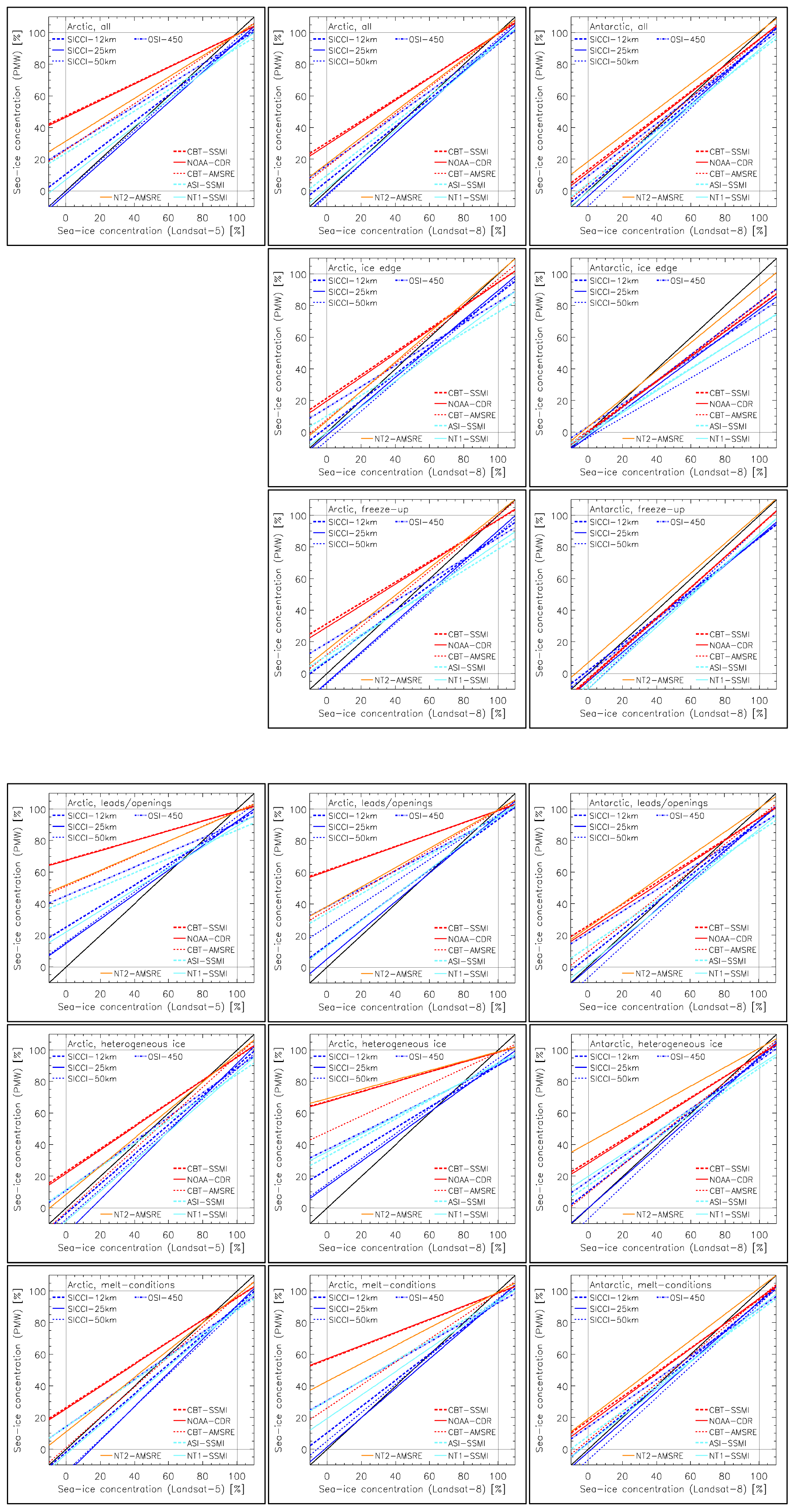
Figure 11Summary of all linear regression lines obtained for the comparison between Landsat SIC and PMW SIC for all ice regimes – except high-concentration ice. Columns denote, from left to right, Landsat-5 Arctic (i.e., first-year ice), Landsat-8 Arctic (i.e., mixed first-year–multiyear ice and multiyear ice), and Landsat-8 Antarctic. Ice regimes are sorted per row from top to bottom. Different colors and line styles denote different products as indicated. The solid black line denotes the identity line. Note “AMSRE” refers to both AMSRE (Landsat-5) and AMSR2 (Landsat-8).
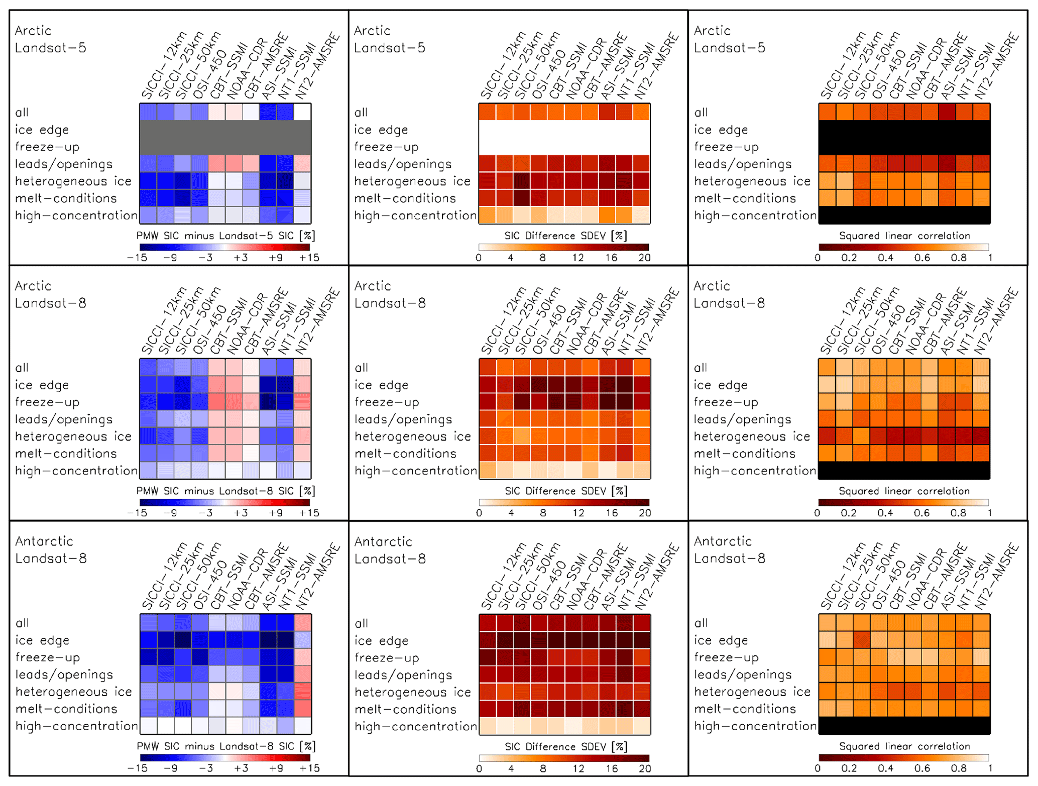
Figure 12Illustration of the statistical parameters of the comparison between Landsat SIC and PMW SIC for all ice regimes. Rows denote, from top to bottom, first-year ice Arctic (Landsat-5), mixed first-year–multiyear ice and multiyear ice Arctic (Landsat-8), and all ice Antarctic (Landsat-8). Columns denote, from left to right, accuracy (difference PMW SIC minus Landsat SIC), precision (standard deviation of the SIC difference), and squared linear correlation coefficient. The uni-colored rows denote cases left out either because these ice regimes are not populated (topmost row of panels) or because the retrieval of parameters did not make sense (squared linear correlation for ice regime “high concentration”). Note “AMSRE” refers to both AMSRE (Landsat-5) and AMSR2 (Landsat-8).
We observe a similar tendency for all other ice regimes where the LSO is applied, e.g., “freeze-up” or “melt conditions”, in the Southern Hemisphere and in the Northern Hemisphere, and for SICCI-25km and SICCI-12km as well (see Tables S4 and S5 in the Supplement). However, we find far fewer SIC data pairs subject to LSO filtering for OSI-450; hence the effect of switching on or off the LSO is comparably small. We hypothesize that this could be explained by the different native resolution of the satellite data used, the different sampling, and the different grid cell size and spacing (see Sect. 5.1). However, testing this hypothesis is beyond the scope of this paper. For the SICCI-2 SIC products, we can confirm the hypothesis that the comparably large number of PMW SIC=0 % or % across basically the entire SIC range (see Figs. 2, 3, and 4, panels a–c) can be explained by the application of an LSO resulting in an elevated number of cases with PMW SIC < Landsat SIC. This provides a viable explanation for unexpectedly large SIC differences observed for SICCI-50km along coastlines, particularly of Greenland or the eastern Antarctic, reported in Kern et al. (2019, their Figs. 8c and 11c). Whether this is due to the land spillover correction at the brightness temperature level (Maass and Kaleschke, 2010) or the statistical filtering (Cavalieri et al., 1999) remains to be investigated. We clearly see it as an advantage to be able to switch off filters and in a reverse-engineering way investigate the impact of these filters for SICCI-2 and OSI-450 products. Application of the LSO can produce an artificially large number of SIC values near or at 0 % that agree less well with the Landsat SIC than the originally retrieved SIC values – as we demonstrate for the SICCI-2 and OSI-450 products. As a consequence, results of an evaluation including a considerable number of near-coastal grid cells need to be interpreted carefully. The number of artificially low SIC values resulting from the LSO for the other six PMW SIC products is unknown as is their impact on the evaluation results shown in this paper.
In this paper, we present results of an evaluation of 10 passive microwave (PMW) SIC products against SIC estimates derived from more than 350 clear-sky Landsat visible images acquired in the Northern Hemisphere during mostly late winter and spring (March through May) and in the Southern Hemisphere during spring, summer, and early fall (October through March). We estimate Landsat SIC at the grid resolution of the PMW SIC products using results of supervised classification of Landsat broadband albedo maps into ice and water at 30 m pixel resolution. The comparison between PMW and Landsat SIC is carried out based on all valid collocated SIC map pairs but also based on subsets of these pairs defining certain ice regimes. These ice regimes are “high concentration”, “freeze-up”, “ice edge”, “leads/openings”, “heterogeneous ice”, and “melt conditions”. Our comparison uses statistical parameters such as the mean difference between PMW and Landsat SIC and its standard deviation, the median difference, and parameters describing the linear agreement: slope and intercept of a linear regression and the linear regression coefficient. We summarize these parameters in Figs. 11 and 12 and make the following conclusions:
-
It is important to take an integrated view of the statistical parameters because, for instance, a small overall bias is not necessarily associated with a good linear agreement across the entire SIC range, and a perfect linear agreement with a slope close to unity and a high correlation could be associated with a large overall bias.
-
It is also important to take into account the expected influences of, e.g., melt conditions (Sect. 4.3) and fraction of new/thin ice (Sect. 4.1), as well as sub-pixel-size ocean–ice mixture (Sect. 2.2.4), on both PMW SIC and Landsat SIC.
-
SICCI-25km and SICCI-50km SIC offer overall the best linear agreement to Landsat SIC as demonstrated in Fig. 11 and the right column of Fig. 12, right column. This is illustrated as well by mean and median PMW SIC values computed for Landsat SIC bins aligned very well along the identity line (Figs. 2–4), with exceptions being explainable by filters applied in the products (see Sect. 5.3). The magnitude of the difference PMW SIC minus Landsat SIC is, however, larger than for the two CBT products and NOAA-CDR, almost without exception (Fig. 12, left column).
-
CBT-SSMI, CBT-AMSR, NOAA-CDR, and NT2-AMSR offer the smallest overall magnitude of the difference PMW SIC minus Landsat SIC (Fig. 12, left column). Except for CBT-AMSR2 in the Southern Hemisphere, mean and median PMW SIC values align less well along the identity line than for SICCI-25km and SICCI-50km in Figs. 2–4. The linear agreement is considerably worse than for SICCI-25km and SICCI-50km (Fig. 11 and right column of Fig. 12).
-
NT2-AMSR is the only product overestimating Landsat SIC in the Southern Hemisphere – overall but also for almost all ice regimes. This is problematic in view of the potential positive bias of Landsat SIC for ice conditions with an elevated number of mixed ocean–ice Landsat pixels (see Sect. 2.2.4), e.g., ice regimes “melt conditions”, “ice edge”, and “freeze-up”.
All products provide SIC data truncated to the range 0 % to 100 %, albeit all algorithms, except NT2-AMSR, use a SIC retrieval procedure which in principle provides a full SIC distribution around the end-members 0 % and 100 %. Only the SICCI-2 products and OSI-450 allow consideration of the full SIC distribution. While our main results are derived with the truncated SIC distribution, we demonstrate that, without exception, using the full SIC distribution reduces the mean difference and enhances the quality of the linear agreement between PMW SIC and Landsat SIC which is already superior for SICCI-25km and SICCI-50km. It is important to consider this observation when comparing the results obtained with the 10 products against each other in order to avoid misinterpretation. While we obtain the smallest SIC differences for CBT-SSMI, CBT-AMSR, NOAA-CDR, and NT2-AMSR, these are likely to change using the full SIC distribution. This applies in particular to ice regimes “high-concentration” (Sect. 4.2) and “melt conditions” but also to the full set of SIC data pairs (denoted “all” in Fig. 12). The impact this difference in the comprehensiveness of the SIC products has on our evaluation results prevents us from making a ranking between the SIC products.
This paper is limited to clear-sky visible imagery. It is hence impossible to evaluate the performance of the SIC products under the full set of possible weather conditions influencing SIC retrieval, i.e., surface wind speed and atmospheric water vapor and cloud liquid water content. Our results likely cover a certain range of surface wind speeds and atmospheric water vapor contents which we, however, did not quantify, e.g., by means of atmospheric reanalysis data, to stay focused. Obviously, this would be an issue worth pursuing in a forthcoming study for which SIC estimates based on SAR data have to be used. These might allow us to assess PMW SIC quality also under higher loads of atmospheric water vapor content and, more importantly, clouds. Such a study could then focus in particular on an improved accuracy assessment of the PMW SIC in the marginal ice zone and along the ice edge. In such regions, our approach to derive Landsat SIC likely results in the highest positive biases – between a few percent to, in the worst case, 20 % for single PMW grid cells – due to mixed ocean–ice Landsat pixels classified as ice. Such a study would also be an excellent opportunity to evaluate the weather filters currently employed in the SIC products. In order to have a meaningful sample, such a study would require an equally extensive data set of SAR images interpreted into well-evaluated SIC estimates. This calls for continued development of reliable and consistent SIC estimates from SAR and thorough evaluation of SAR SIC products in both hemispheres.
Except SICCI-12km all sea-ice concentration products are publicly available under the following references: SICCI-25km (https://doi.org/10.5285/f17f146a31b14dfd960cde0874236ee5; Pedersen et al., 2017a), SICCI-50km (https://doi.org/10.5285/5f75fcb0c58740d99b07953797bc041e; Pedersen et al., 2017b), OSI-450 (https://doi.org/10.15770/EUM_SAF_OSI_0008 and https://osi-saf.eumetsat.int/products/osi-430-b-complementing-osi-450; OSI SAF, 2017a, b), ASI-SSMI (Kern et al., 2020a), NOAA-CDR, NT1-SSMI, and CBT-SSMI (https://doi.org/10.7265/N59P2ZTG; Meier et al., 2017), and CBT-AMSR and NT2-AMSR (https://doi.org/10.5067/TRUIAL3WPAUP; Meier et al., 2018). The SICCI-12km product is available upon request from Thomas Lavergne. The classified Landsat images are available from https://doi.org/10.25592/uhhfdm.9181 (Kern, 2021).
The supplement related to this article is available online at: https://doi.org/10.5194/tc-16-349-2022-supplement.
SK wrote the manuscript. TL, LTP, and RTT contributed to the concept and work presented in the paper and also assisted in the writing. SK performed the data analysis together with LB, MM, and LZ. SK conducted the intercomparison with contributions in the interpretation of the results from TL, LTP, and RTT.
The contact author has declared that neither they nor their co-authors have any competing interests.
Publisher's note: Copernicus Publications remains neutral with regard to jurisdictional claims in published maps and institutional affiliations.
The publication contributes to the Cluster of Excellence “CLICCS – Climate, Climatic Change, and Society” and to the Center for Earth System Research and Sustainability (CEN) of the University of Hamburg. We are very grateful for the very helpful comments given by two anonymous reviewers and by the scientific editor Chris Derksen.
The work presented here was funded by EUMETSAT (through the 3rd Continuous Developments and Operation Phase of OSI SAF) and ESA (through the Climate Change Initiative Sea_Ice_cci project). The ESA Climate Change Initiative (CCI+) Sea Ice Phase 1 activity (contract no. 4000126449/19/I-NB) contributed to the article processing charges of this paper.
This paper was edited by Chris Derksen and reviewed by two anonymous referees.
Andersen, S., Tonboe, R. T., Kern, S., and Schyberg, H.: Improved retrieval of sea ice total concentration from spaceborne passive microwave observations using Numerical Weather Prediction model fields: An intercomparison of nine algorithms, Remote Sens. Environ., 104, 374–392, 2006.
Andersen, S., Pedersen, L. T., Heygster, G., Tonboe, R. T., and Kaleschke, L.: Intercomparison of passive microwave sea ice concentration retrievals over the high concentration Arctic sea ice, J. Geophys. Res., 112, C08004, https://doi.org/10.1029/2006JC003543, 2007.
Barsi, J. A., Kenton, L., Kvaran, G., Markham, B. L., and Pedelty, J. A.: The spectral response of the Landsat-8 operational land imager, Remote Sens., 6, 10232–10251, https://doi.org/10.3390/rs61010232, 2014.
Belchansky, G. I. and Douglas, D. C.: Seasonal comparisons of sea ice concentration estimates derived from SSM/I, OKEAN, and RADARSAT data, Remote Sens. Environ., 81, 67–81, 2002.
Boulze, H., Korosov, A., and Brajard, J.: Classification of sea ice types in Sentinel-1 SAR using convolutional neural networks, Remote Sens., 12, 2165–2184, https://doi.org/10.3390/rs12132165, 2020.
Boutin, G., Lique, C., Ardhuin, F., Rousset, C., Talandier, C., Accensi, M., and Girard-Ardhuin, F.: Towards a coupled model to investigate wave–sea ice interactions in the Arctic marginal ice zone, The Cryosphere, 14, 709–735, https://doi.org/10.5194/tc-14-709-2020, 2020.
Brandt, R. E., Warren, S. G., Worby, A. P., and Grenfell, T. C.: Surface Albedo of the Antarctic sea ice zone, J. Climate, 18, 3606–3622, 2005.
Burgard, C., Notz, D., Pedersen, L. T., and Tonboe, R. T.: The Arctic Ocean Observation Operator for 6.9 GHz (ARC3O) – Part 1: How to obtain sea ice brightness temperatures at 6.9 GHz from climate model output, The Cryosphere, 14, 2369–2386, https://doi.org/10.5194/tc-14-2369-2020, 2020.
Cavalieri, D. J.: A microwave technique for mapping thin sea ice, J. Geophys. Res., 99, 12561–12572, 1994.
Cavalieri, D. J., Gloersen, P., and Campbell, W. J.: Determination of Sea Ice Parameters with the NIMBUS 7 SMMR, J. Geophys. Res., 89, 5355–5369, 1984.
Cavalieri, D. J., Crawford, J., Drinkwater, M., Emery, W. J., Eppler, D. T., Farmer, L. D., Goodberlet, M., Jentz, R., Milman, A., Morris, C., Onstott, R., Schweiger, A., Shuchman, R., Steffen, K., Swift, C. T., Wackerman, C., and Weaver, R. L.: NASA sea ice validation program for the DMSP SSM/I: final report. NASA Technical Memorandum 104559, National Aeronautics and Space Administration, Washington, D. C., 126 pp., 1992.
Cavalieri, D. J., Parkinson, C. L., Gloersen, P., Comiso, J. C., and Zwally, H. J.: Deriving long-term time series of sea ice cover from satellite passive-microwave multisensor data sets, J. Geophys. Res., 104, 15803–15814, https://doi.org/10.1029/1999JC900081, 1999.
Cavalieri, D. J., Markus, T., Hall, D. K., Gasiewski, A. J., Klein, M., and Ivanoff, A.: Assessment of EOS Aqua AMSR-E Arctic sea ice concentrations using Landsat-7 and airborne microwave imagery, IEEE T. Geosci. Remote, 44, 3057–3069, https://doi.org/10.1109/TGRS.2006.878445, 2006.
Chander, G., Markham, B. L., and Barsi, J. A.: Revised Landsat-5 Thematic Mapper Radiometric Calibration, IEEE Geosci. Remote S., 4, 490–494, 2007.
Chander, G., Markham, B. L., and Helder, D. L.: Summary of current radiometric calibration coefficients for Landsat MSS, TM, ETM+, and EO-1 ALI sensors, Remote Sens. Environ., 113, 893–903, 2009.
Cheng, A., Casati, B., Tivy, A., Zagon, T., Lemieux, J.-F., and Tremblay, L. B.: Accuracy and inter-analyst agreement of visually estimated sea ice concentrations in Canadian Ice Service ice charts using single-polarization RADARSAT-2, The Cryosphere, 14, 1289–1310, https://doi.org/10.5194/tc-14-1289-2020, 2020.
Comiso, J. C.: Characteristics of arctic winter sea ice from satellite multispectral microwave observations, J. Geophys. Res., 91, 975–994, 1986.
Comiso, J. C.: Enhanced sea ice concentrations and ice extents from AMSR-E data, J. Rem. Sens. Soc. Japan, 29, 199–215, 2009.
Comiso, J. C. and Nishio, F.: Trends in the sea ice cover using enhanced and compatible AMSR-E, SSM/I, and SMMR data, J. Geophys. Res., 113, C02S07, https://doi.org/10.1029/2007JC004257, 2008.
Comiso, J. C. and Steffen, K.: Studies of Antarctic sea ice concentrations from satellite data and their applications, J. Geophys. Res., 106, 31361–31385, 2001.
Comiso, J. C. and Zwally, H. J.: Antarctic sea ice concentrations inferred from Nimbus 5 ESMR and Landsat imagery, J. Geophys. Res., 87, 5836–5844, https://doi.org/10.1029/JC087iC08p05836, 1982.
Comiso, J. C., Wadhams, P., Krabill, W. B., Swift, R. N., Crawford, J. P., and Tucker III, W. B.: Top/bottom multisensory remote sensing of Arctic sea ice, J. Geophys. Res., 96, 2693–2709, https://doi.org/10.1029/90JC02466, 1991.
Comiso, J. C., Cavalieri, D. J., Parkinson, C. L., and Gloersen, P.: Passive microwave algorithms for sea ice concentration: A comparison of two techniques, Remote Sens. Environ., 60, 357–384, 1997.
Comiso, J. C., Cavalieri, D. J., and Markus, T.: Sea ice concentration, ice temperature, and snow depth, using AMSR-E data, IEEE T. Geosci. Remote, 41, 243–252, https://doi.org/10.1109/TGRS.2002.808317, 2003.
Cooke, C. L. V. and Scott, K. A.: Estimating sea ice concentration from SAR: Training convolutional neural networks with passive microwave data, IEEE T. Geosci. Remote, 57, 4735–4747, https://doi.org/10.1109/TGRS.2019.2892723, 2019.
Dokken, S. T., Håkansson, B., and Askne, J.: Inter-comparison of Arctic sea ice concentration using RADARSAT, ERS, SSM/I and In-Situ Data, Can. J. Remote Sens., 26, 521–536, https://doi.org/10.1080/07038992.2000.10874793, 2000.
Drusch, M., Del Bello, U., Carlier, S., Colin, O., Fernandez, V., Gascon, F., Hoersch, B., Isola, C., Laberinti, P., Martimort, P., Meygret, A., Spoto, F., Sy, O., Marchese, F., and Bargellini, P.: Sentinel-2: ESA's optical high-resolution mission for GMES operational services, Remote Sens. Environ., 120, 25–36, https://doi.org/10.1016/j.rse.2011.11.026, 2012.
Ezraty, R., Girard-Ardhuin, F., Piollé, J.-F., Kaleschke, L., and Heygster, G.: Arctic and Antarctic sea ice concentration and Arctic sea ice drift estimated from special sensor microwave data – Users's Manual, Version 2.1, IFREMER, Brest, France, February 2007.
Han, H. and Kim, H.-C.: Evaluation of summer passive microwave sea ice concentrations in the Chukchi Sea based on KOMPSAT-5 SAR and numerical weather prediction data, Remote Sens. Environ., 209, 343–362, https://doi.org/10.1016/j.rse.2018.02.058, 2018.
Heinrichs, J. F., Cavalieri, D. J., and Markus, T.: Assessment of the AMSR-E sea ice concentration product at the ice edge using RADARSAT-1 and MODIS imagery, IEEE T. Geosci. Remote, 44, 3070–3080, https://doi.org/10.1109/TGRS.2006.880622, 2006.
Ivanova, N., Johannessen, O. M., Pedersen, R. T., and Tonboe, R. T.: Retrieval of Arctic sea ice parameters by satellite passive microwave sensors: A comparison of eleven sea ice concentration algorithms, IEEE T. Geosci. Remote, 52, 7233–7246, https://doi.org/10.1109/TGRS.2014.2310136, 2014.
Ivanova, N., Pedersen, L. T., Tonboe, R. T., Kern, S., Heygster, G., Lavergne, T., Sørensen, A., Saldo, R., Dybkjær, G., Brucker, L., and Shokr, M.: Inter-comparison and evaluation of sea ice algorithms: towards further identification of challenges and optimal approach using passive microwave observations, The Cryosphere, 9, 1797–1817, https://doi.org/10.5194/tc-9-1797-2015, 2015.
Kaleschke, L., Lüpkes, C., Vihma, T., Haarpaintner, J., Bochert, A., Hartmann, J., and Heygster, G.: SSM/I sea ice remote sensing for mesoscale ocean-atmosphere interaction analysis, Can. J. Remote Sens., 27, 526–537, 2001.
Karvonen, J.: A sea ice concentration estimation algorithm utilizing radiometer and SAR data, The Cryosphere, 8, 1639–1650, https://doi.org/10.5194/tc-8-1639-2014, 2014.
Karvonen, J.: Baltic sea ice concentration estimation using SENTINEL-1 SAR and AMSR2 microwave radiometer data, IEEE T. Geosci. Remote, 55, 2871–2883, https://doi.org/10.1109/TGRS.2017.2655567, 2017.
Kern, S.: A new method for medium-resolution sea ice analysis using weather-influence corrected Special Sensor Microwave/Imager 85 GHz data, Int. J. Remote Sens., 25, 4555–4582, 2004.
Kern, S.: Landsat surface type over water from supervised classification of surface broadband albedo estimates (Version 2021_fv0.01), Universität Hamburg [data set], https://doi.org/10.25592/uhhfdm.9181, 2021.
Kern, S., Rösel, A., Pedersen, L. T., Ivanova, N., Saldo, R., and Tonboe, R. T.: The impact of melt ponds on summertime microwave brightness temperatures and sea-ice concentrations, The Cryosphere, 10, 2217–2239, https://doi.org/10.5194/tc-10-2217-2016, 2016.
Kern, S., Lavergne, T., Notz, D., Pedersen, L. T., Tonboe, R. T., Saldo, R., and Sørensen, A. M.: Satellite passive microwave sea-ice concentration data set intercomparison: closed ice and ship-based observations, The Cryosphere, 13, 3261–3307, https://doi.org/10.5194/tc-13-3261-2019, 2019.
Kern, S., Kaleschke, L., Girard-Ardhuin, F., Spreen, G., and Beitsch, A.: Global daily gridded 5 d median-filtered, gap-filled ASI Algorithm SSMI-SSMIS sea ice concentration data, Integrated Climate Date Center (ICDC), CEN, University of Hamburg, Germany [data set], available at: https://www.cen.uni-hamburg.de/en/icdc/data/cryosphere/seaiceconcentration-asi-ssmi.html (last access: 9 December 2021), 2020a.
Kern, S., Lavergne, T., Notz, D., Pedersen, L. T., and Tonboe, R.: Satellite passive microwave sea-ice concentration data set inter-comparison for Arctic summer conditions, The Cryosphere, 14, 2469–2493, https://doi.org/10.5194/tc-14-2469-2020, 2020b.
Knap, W. H., Brock, B. W., Oerlemans, J., and Willis, I. C.: Comparison of Landsat TM-derived and ground-based albedos of Haut Glacier d'Arolla, Switzerland, Int. J. Remote Sens., 20, 3293–3310, 1999.
Koepke, P.: Removal of Atmospheric Effects from AVHRR albedos, J. Appl. Meteorol., 28, 1341–1348, 1989.
Komarov, A. S. and Buehner, M.: Automated detection of ice and open water from dual-polarization RADARSAT-2 images for data assimilation, IEEE T. Geosci. Remote, 55, 5755–5769, https://doi.org/10.1109/TGRS.2017.2713987, 2017.
Komarov, A. S. and Buehner, M.: Improved retrieval of ice and open water from sequential RADARSAT-2 images, IEEE T. Geosci. Remote, 57, 3694–3702, https://doi.org/10.1109/TGRS.2018.2886685, 2019.
Kwok, R.: Sea ice concentration estimates from satellite passive microwave radiometry and openings from SAR ice motion, Geophys. Res. Lett., 29, 1311, https://doi.org/10.1029/2002GL014787, 2002.
Lavergne, T., Sørensen, A. M., Kern, S., Tonboe, R., Notz, D., Aaboe, S., Bell, L., Dybkjær, G., Eastwood, S., Gabarro, C., Heygster, G., Killie, M. A., Brandt Kreiner, M., Lavelle, J., Saldo, R., Sandven, S., and Pedersen, L. T.: Version 2 of the EUMETSAT OSI SAF and ESA CCI sea-ice concentration climate data records, The Cryosphere, 13, 49–78, https://doi.org/10.5194/tc-13-49-2019, 2019.
Leigh, S., Wang, Z., and Clausi, D. A.: Automated ice-water classification using dual polarization SAR satellite imagery, IEEE T. Geosci. Remote, 52, 5529–5539, https://doi.org/10.1109/TGRS.2013.2290231, 2014.
Liu, Y., Key, J., and Mahoney, R.: Sea and freshwater ice concentration from VIIRS on Suomi NPP and the future JPSS satellites, Remote Sens., 8, 523–542, https://doi.org/10.3390/rs8060523, 2016.
Lohse, J., Doulgeris, A. P., and Dierking, W.: An optimal decision-tree design strategy and its application to sea ice classification from SAR imagery, Remote Sens., 11, 1574–1588, https://doi.org/10.3390/rs11131574, 2019.
Lu, J., Heygster, G., and Spreen, G.: Atmospheric correction of sea-ice concentration retrieval for 89 GHz AMSR-E observations, IEEE J. Sel. Top. Appl., 11, 1442–1457, https://doi.org/10.1109/JSTARS.2018.2805193, 2018.
Lu, P., Li, Z. L., Zhang, Z. H., and Dong, X. L.: Aerial observations of floe size distributions in the marginal ice zone of summer Prydz Bay, J. Geophys. Res., 113, C02011, https://doi.org/10.1029/2006JC003965, 2008.
Ludwig, V., Spreen, G., and Pedersen, L. T.: Evaluation of a new merged sea-ice concentration dataset at 1 km resolution from thermal infrared and passive microwave satellite data in the Arctic, Remote Sens., 12, 3183–3210, https://doi.org/10.3390/rs12193183, 2020.
Maass, N. and Kaleschke, L.: Improving passive microwave sea ice concentration algorithms for coastal areas: applications to the Baltic Sea, Tellus A, 62, 393–410, https://doi.org/10.1111/j.1600-0870.2010.00452.x, 2010.
Malmgren-Hansen, D., Pedersen, L. T., Aasbjerg Nielsen, A., Brandt Kreiner, M., Saldo, R., Skriver, H., Lavelle, J., Buus-Hinkler, J., and Harnvig Krane, K.: A convolutional neural network architecture for sentinel-1 and AMSR2 data fusion, IEEE T. Geosci. Remote, 59, 1890–1902, https://doi.org/10.1109/TGRS.2020.3004539, 2020.
Marcq, S. and Weiss, J.: Influence of sea ice lead-width distribution on turbulent heat transfer between the ocean and the atmosphere, The Cryosphere, 6, 143–156, https://doi.org/10.5194/tc-6-143-2012, 2012.
Markus, T. and Cavalieri, D. J.: An enhancement of the NASA Team sea ice algorithm, IEEE T. Geosci. Remote, 38, 1387–1398, 2000.
Markus, T. and Cavalieri, D. J.: The AMSR-E NT2 sea ice concentration algorithm: its basis and implementation, J. Rem. Sens. Soc. Japan, 29, 216–225, 2009.
Meier, W. N. and Windnagel, A.: Sea ice concentration – climate algorithm theoretical basis document, NOAA Climate Data Record Program CDRP-ATBD-0107 Rev. 7 (03/06/2018), available at: https://www.ncdc.noaa.gov/cdr/oceanic/sea-ice-concentration (last access: 19 February 2020), 2018.
Meier, W. N., Fetterer, F., Savoie, M., Mallory, S., Duerr, R., and Stroeve, J.: NOAA/NSIDC Climate Data Record of Passive Microwave Sea Ice Concentration, Version 3, NSIDC: National Snow and Ice Data Center, Boulder, Colorado USA [data set], https://doi.org/10.7265/N59P2ZTG, 2017.
Meier, W. N., Markus, T., and Comiso, J. C.: AMSR-E/AMSR2 Unified L3 Daily 25.0 km Brightness Temperatures, Sea Ice Concentration, Motion & Snow Depth Polar Grids, Version 1, Boulder, Colorado, USA, NASA National Snow and Ice Data Center Distributed Active Archive Center [data set], https://doi.org/10.5067/TRUIAL3WPAUP, 2018.
Meier, W. N., Fetterer, F., Windnagel, A. K., and Stewart, S.: NOAA/NSIDC Climate Data Record of Passive Microwave Sea Ice Concentration, Version 4. Boulder, Colorado USA. NSIDC: National Snow and Ice Data Center https://doi.org/10.7265/efmz-2t65, 2021.
Mojica Moncada, J. F. and Holland, D.: Automatic Weather Station Pine Island Glacier, U. S. Antarctic Program (USAP) Data Center, https://doi.org/10.15784/601216, 2019.
Nose, T., Waseda, T., Kodaira, T., and Inoue, J.: Satellite-retrieved sea ice concentration uncertainty and its effect on modelling wave evolution in marginal ice zones, The Cryosphere, 14, 2029–2052, https://doi.org/10.5194/tc-14-2029-2020, 2020.
Ochilov, S. and Clausi, D. A.: Operational SAR sea-ice image classification, IEEE T. Geosci. Remote, 50, 4397–4408, https://doi.org/10.1109/TGRS.2012.2192278, 2012.
Onana, V.-De-P., Kurtz, N. T., Farrell, S. L., Koenig, L. S., Studinger, M., and Harbeck, J. P.: A sea-ice lead detection algorithm for use with high-resolution airborne visible imagery, IEEE T. Geosci. Remote, 51, 38–56, https://doi.org/10.1109/TGRS.2012.2202666, 2013.
OSI SAF: Global Sea Ice Concentration Climate Data Record v2.0 – Multimission, EUMETSAT SAF on Ocean and Sea Ice [data set], https://doi.org/10.15770/EUM_SAF_OSI_0008, 2017a.
OSI SAF: Global Sea Ice Concentration Interim Climate Data Record 2016–onwards (v2.0, 2017), OSI-430-b [data set], https://osi-saf.eumetsat.int/products/osi-430-b-complementing-osi-450 (last access: 17 September 2021), 2017b.
Ozsoy-Cicek, B., Xie, H., Ackley, S. F., and Ye, K.: Antarctic summer sea ice concentration and extent: comparison of ODEN 2006 ship observations, satellite passive microwave and NIC sea ice charts, The Cryosphere, 3, 1–9, https://doi.org/10.5194/tc-3-1-2009, 2009.
Paget, M. J., Worby, A. P., and Michael, K. J.: Determining the floe-size distribution of East Antarctic sea ice from digital aerial photographs, Ann. Glaciol., 33, 94–100, 2001.
Pedersen, L. T., Dybkjær, G., Eastwood, S., Heygster, G., Ivanova, N., Kern, S., Lavergne, T., Saldo, R., Sandven, S., Sørensen, A., and Tonboe, R. T.: ESA Sea Ice Climate Change Initiative (Sea_Ice_cci): Sea Ice Concentration Climate Data Record from the AMSR-E and AMSR-2 instruments at 25 km grid spacing, version 2.1, Centre for Environmental Data Analysis [data set], 5 October 2017, https://doi.org/10.5285/f17f146a31b14dfd960cde0874236ee5, 2017a.
Pedersen, L. T., Dybkjær, G., Eastwood, S., Heygster, G., Ivanova, N., Kern, S., Lavergne, T., Saldo, R., Sandven, S., Sørensen, A., and Tonboe, R. T.: ESA Sea Ice Climate Change Initiative (Sea_Ice_cci): Sea Ice Concentration Climate Data Record from the AMSR-E and AMSR-2 instruments at 50 km grid spacing, version 2.1, Centre for Environmental Data Analysis, 5 October 2017, Centre for Environmental Data Analysis [data set], https://doi.org/10.5285/5f75fcb0c58740d99b07953797bc041e, 2017b.
Pegau, W. S. and Paulson, C. A.: The albedo of Arctic leads in summer, Ann. Glaciol., 33, 221–224, 2001.
Peng, G., Meier, W. N., Scott, D. J., and Savoie, M. H.: A long-term and reproducible passive microwave sea ice concentration data record for climate studies and monitoring, Earth Syst. Sci. Data, 5, 311–318, https://doi.org/10.5194/essd-5-311-2013, 2013.
Perovich, D. K. and Jones, K. F.: The seasonal evolution of sea ice floe size distribution, J. Geophys. Res.-Oceans, 119, 8767–8777, https://doi.org/10.1002/2014JC010136, 2014.
Shi, Q., Su, J., Heygster, G., Shi, J., Wang, L., Zhu, L., Lou, Q., and Ludwig, V.: Step-by-step validation of Antarctic ASI AMSR-E sea-ice concentrations by MODIS and an aerial image, IEEE T. Geosci. Remote, 59, 392–403, https://doi.org/10.1109/TGRS.2020.2989037, 2021.
Shokr, M. and Agnew, T. A.: Validation and potential applications of Environment Canada Ice Concentration Extractor (ECICE) algorithm to Arctic ice by combining AMSR-E and QuikSCAT observations, Remote Sens. Environ., 128, 315–332, https://doi.org/10.1016/j.rse.2012.10.016, 2013.
Shokr, M. and Markus, T.: Comparison of NASA Team2 and AES-York ice concentration algorithms against operational ice charts from the Canadian Ice Service, IEEE T. Geosci. Remote, 44, 2164–2175, https://doi.org/10.1109/TGRS.2006.872077, 2006.
Singha, S., Johansson, M., Hughes, N., Hvidegaard, S. M., and Skourup, H.: Arctic sea ice characterization using spaceborne fully polarimetric L-, C-, and X-band SAR with validation by airborne measurements, IEEE T. Geosci. Remote, 56, 3715–3734, https://doi.org/10.1109/TGRS.2018.2809504, 2018.
Spreen, G., Kaleschke, L., and Heygster, G.: Sea ice remote sensing using AMSR-E 89 GHz channels, J. Geophys. Res., 113, C02S03, https://doi.org/10.1029/2005JC003384, 2008.
Steer, A., Worby, A. P., and Heil, P.: Observed changes in sea-ice floe size distribution during early summer in the western Weddell Sea, Deep-Sea Res. Pt. II, 55, 933–942, https://doi.org/10.1016/j.dsr2.2007.12.016, 2008.
Steffen, K. and Maslanik, J. A.: Comparison of Nimbus 7 scanning multichannel microwave radiometer radiance and derived sea ice concentrations with Landsat imagery for the north water area of Baffin Bay, J. Geophys. Res., 93, 10769–10781, https://doi.org/10.1029/JC093iC09p10769, 1988.
Steffen, K. and Schweiger, A.: NASA team algorithm for sea ice concentration retrieval from Defense Meteorological Satellite Program special sensor microwave imager: comparison with Landsat satellite data, J. Geophys. Res., 96, 21971–21987, 1991.
Titchner, H. A. and Rayner, N. A.: The Met Office Hadley Centre sea ice and sea surface temperature data set, version 2: 1. Sea Ice concentrations, J. Geophys. Res.-Atmos., 119, 2864–2889, https://doi.org/10.1002/2013JD020316, 2014.
Tonboe, R. T., Eastwood, S., Lavergne, T., Sørensen, A. M., Rathmann, N., Dybkjær, G., Pedersen, L. T., Høyer, J. L., and Kern, S.: The EUMETSAT sea ice concentration climate data record, The Cryosphere, 10, 2275–2290, https://doi.org/10.5194/tc-10-2275-2016, 2016.
Toyota, T., Haas, C., and Tamura, T.: Size distribution and shape properties of relatively small sea-ice floes in the Antarctic marginal ice zone in late winter, Deep-Sea Res. Pt. II, 58, 1182–1193, https://doi.org/10.1016/j.dsr2.2010.10.034, 2011.
Toyota, T., Kohout, A., and Fraser, A. D.: Formation processes of sea ice floe size distribution in the interior pack and its relationship to the marginal ice zone off East Antarctica, Deep-Sea Res. Pt. II, 131, 28–40, https://doi.org/10.1016/j.dsr2.2015.10.003, 2016.
Tschudi, M. A., Curry, J. A., and Maslanik, J. A.: Characterization of springtime leads in the Beaufort/Chukchi Seas from airborne and satellite observations during FIRE/SHEBA, J. Geophys. Res., 107, 8034, https://doi.org/10.1029/2000JC000541, 2002.
Wang, L., Scott, K. A., Xu, L., and Clausi, D. A.: Sea ice concentration estimation during melt from dual-pol SAR scenes using deep convolutional neural networks: A case study, IEEE T. Geosci. Remote, 54, 4524–4533, https://doi.org/10.1109/TGRS.2016.2543660, 2016.
USGS: Landsat 8 (L8) Data Users Handbook, LSDS-1574, Version 5.0, November 2019, Department of the Interior, U.S. Geological Survey, EROS, Sioux Falls, South Dakota, 2019.
Wang, L., Scott, K. A., and Clausi, D. A.: Sea ice concentration estimation during freeze-up from SAR imagery using a convolutional neural network, Remote Sens., 9, 408–427, https://doi.org/10.3390/rs9050408, 2017.
Wang, Y.-R. and Li, X.-M.: Arctic sea ice cover data from spaceborne synthetic aperture radar by deep learning, Earth Syst. Sci. Data, 13, 2723–2742, https://doi.org/10.5194/essd-13-2723-2021, 2021.
Wensnahan, M., Maykut, G. A., Grenfell, T. C., and Winebrenner, D. P.: Passive microwave remote sensing of thin sea ice using principal component analysis, J. Geophys. Res., 98, 12453–12468, https://doi.org/10.1029/93JC00939, 1993.
Wiebe, H., Heygster, G., and Markus, T.: Comparison of the ASI ice concentration algorithm with Landsat-7 ETM+ and SAR imagery, IEEE T. Geosci. Remote, 47, 3008–3015, https://doi.org/10.1109/TGRS.2009.2026367, 2009.
Willmes, S., Nicolaus, M., and Haas, C.: The microwave emissivity variability of snow covered first-year sea ice from late winter to early summer: a model study, The Cryosphere, 8, 891–904, https://doi.org/10.5194/tc-8-891-2014, 2014.
Worby, A. P. and Comiso, J. C.: Studies of the Antarctic sea ice edge and ice extent from satellite and ship observations, Remote Sens. Environ., 92, 98–111, https://doi.org/10.1016/j.rse.2004.05.007, 2004.
Zakhvatkina, N., Korosov, A., Muckenhuber, S., Sandven, S., and Babiker, M.: Operational algorithm for ice–water classification on dual-polarized RADARSAT-2 images, The Cryosphere, 11, 33–46, https://doi.org/10.5194/tc-11-33-2017, 2017.
Zatko, M. C. and Warren, S. G.: East Antarctic sea ice in spring: spectral albedo of snow, nilas, frost flowers and slush, and light-absorbing impurities in snow, Ann. Glaciol., 56, 53–64, https://doi.org/10.3189/2015AoG69A574, 2015.
Zhang, Q. and Skjetne, R.: Image processing for identification of sea-ice floes and the floe size distributions, IEEE T. Geosci. Remote, 53, 2913–2924, https://doi.org/10.1109/TGRS.2014.2366640, 2015.
Zhao, X., Chen, Y., Kern, S., Qu, M., Ji, Q., Fan, P., and Liu, Y.: Sea ice concentration derived from FY-3D MWRI and its accuracy assessment, IEEE T. Geosci. Remote, 60, 4300418, https://doi.org/10.1109/TGRS.2021.3063272, 2022.