Large-scale snow data assimilation using a spatialized particle filter: recovering the spatial structure of the particles

Data assimilation is an essential component of any hydrological forecasting system. Its purpose is to incorporate some observations from the field when they become available in order to correct the state variables of the model prior to the forecasting phase. The goal is to ensure that the forecasts are initialized from state variables that are as representative of reality as possible, and also to estimate the uncertainty of the state variables. There are several data assimilation methods, and particle filters are increasingly popular because of their minimal assumptions. The baseline idea is to produce an ensemble of scenarios (i.e. the particles) using perturbations of the forcing variables and/or state variables of the model. The different particles are weighted using the observations when they become available. However, implementing a particle filter over a domain with large spatial dimensions remains challenging, as the number of required particles rises exponentially as the domain size increases. Such a situation is referred to as the “curse of dimensionality”, or a “dimensionality limit”. A common solution to overcome this curse is to localize the particle filter. This consists in dividing the large spatial domain into smaller portions, or “blocks”, and applying the particle filter separately for each block. This can solve the above-mentioned dimensionality problem because it reduces the spatial scale at which each particle filter must be applied. However, it can also cause spatial discontinuities when the blocks are reassembled to form the whole domain. This issue can become even more problematic when additional data are assimilated. The purpose of this study is to test the possibility of remedying the spatial discontinuities of the particles by locally reordering them.

We implement a spatialized particle filter to estimate the snow water equivalent (SWE) over a large territory in eastern Canada by assimilating local SWE observations from manual snow surveys. We apply two reordering strategies based on (1) a simple ascending-order sorting and (2) the Schaake shuffle and evaluate their ability to maintain the spatial structure of the particles. To increase the amount of assimilated data, we investigate the inclusion of a second data set (SR50), in which the SWE is indirectly estimated from automatic measurements of snow depth using sonic sensors. The two reordering solutions maintain the spatial structure of the individual particles throughout the winter season, which significantly reduces the spatial random noise in the distribution of the particles and decreases the uncertainty associated with the estimation. The Schaake shuffle proves to be a better tool for maintaining a realistic spatial structure for all particles, although we also found that sorting provides a simpler and satisfactory solution. The assimilation of the secondary data set improved SWE estimates in ungauged sites when compared with the deterministic model, but we noted no significant improvement when both snow courses and the SR50 data were assimilated.

1 Introduction

The accumulation and melting of snow dominate the hydrology of Nordic and mountainous regions (Doesken and Judson, 1997; Barnett et al., 2005; Hock et al., 2006). In these regions, accurate information about the snow water equivalent (SWE) is crucial for streamflow forecasting (Li and Simonovic, 2002) and reservoir management (Schaefli et al., 2007). Over large territories or catchments, the spatial distribution of SWE can be assessed using remote sensing (Goïta et al., 2003) or snow modelling (Marks et al., 1999; Ohmura, 2001; Essery et al., 2013). The advantages of snow modelling include the possibility to generalize over large territories and ensure complete temporal coverage with a resolution determined by the user. However, as with any kind of model, snow modelling is subject to uncertainty and inaccuracy stemming from errors in the inputs or the model structure itself (structural uncertainty). The origin of structural uncertainty includes both epistemic uncertainty and one's perceptual model (Beven, 2012). Those factors, in addition to tradition (or “legacy”; see, for instance, Addor and Melsen, 2019) influence one's choice of model algorithmic structure, level of complexity and process description (e.g. Clark et al., 2011).

Given that SWE is a cumulative variable, these errors obviously increase in importance throughout the winter, making SWE estimates highly uncertain at the beginning of the melting season. Nonetheless, a correct assessment of the spatial distribution of SWE over large domains is often required for diverse applications, including flood forecasting in large catchments. Therefore, any data assimilation technique for snow that can be applied to such a large spatial domain with satisfactory results is of very high practical importance for operational hydrology, as it could potentially improve flood forecasting and reservoir management.

Data assimilation can be used to limit the accumulation of uncertainty and error from input data and models. The general idea is to correct the state variables of the model using the observations when they become available. Several elaborate data assimilation schemes have been proposed in the literature to deal with these limitations, including optimal interpolation (Burgess and Webster, 1980), ensemble Kalman filtering (Evensen, 2003) and particle filtering (Gordon et al., 1993; Moradkhani et al., 2005). The latter relies on fewer hypotheses than the other schemes in relation to the nonlinearity and non-normality of the uncertainty distributions of the model's input variables, state variables and outputs. The particle filter (PF) is based on the simulation and weighting of different scenarios (particles) rather than modifying the state variables of the model; thus, the physical consistency of state variables is ensured and the disruption of cross-correlations between state variables is avoided. These scenarios are generated within the range of uncertainty of the input data and/or the model structure. Assessing or defining the range of uncertainty for each variable is not a trivial task, but it is also not unique to the particle filter (see, for instance, Thiboult and Anctil, 2015). The particles are weighted using the observations when they become available. These weights can be used to build the distribution of the variable of interest (model output).

A common limitation of the PF is the risk of particle degeneracy. After a certain number of time steps, the evolution of most particles brings them so far from the observation that they are associated with a weight close to zero. This can be seen as an impoverishment of the filter with fewer and fewer useful particles. At some point, a single particle concentrates all the weight, and a distribution can no longer be built. This degeneracy can be avoided using some kind of particle resampling; the particles with the lowest weights are discarded, whereas the better ones are duplicated. Several resampling algorithms have been proposed in the literature, such as those of Gordon et al. (1993); Douc and Cappe (2005); Leisenring and Moradkhani (2011).

The PF has been successfully used for the local (onsite) assimilation of snow data (Leisenring and Moradkhani, 2011; Magnusson et al., 2017). The application of PF over large territories, however, remains challenging. The number of particles must grow exponentially with the dimension of the observed space to avoid filter degeneracy (Snyder et al., 2015). This “curse of dimensionality” (Bengtsson et al., 2008) is a severe drawback for the application of the PF over large spatial domains with a consequent number of observations.

Several procedures have been proposed to overcome the curse of dimensionality. A first approach, known as error inflation (Larue et al., 2018), consists of increasing the error associated with the observation to make the filter more tolerant. Cluzet et al. (2021) proposed a generalization of this approach to apply it over large domains. The most common approach to overcome the curse of dimensionality is localization (Farchi and Bocquet, 2018). This family of methods assumes that points separated by a sufficiently large distance are independent. Then, given this independence, the assimilation is performed locally; that is to say, only observations close enough to a given site of interest are considered. This can be achieved with techniques such as a spatially limited block (where the space is divided into fixed spatial tiles) or localization radius (where observations are selected in a site-specific manner for each site of interest). In this way, the impact of each observation is limited in space, and the assimilation is performed on several subregions with lower spatial dimensions.

Recent work involving spatialization of the PF for assimilating SWE over large spatial domains includes that of Cluzet et al. (2021), who developed the k-local framework to select the appropriate data set to be assimilated for each site of interest; this selection is based on the cross-correlation between ensemble values at the site of interest and observation sites. Poterjoy (2016) introduced a Bayesian updating of particles near observation sites while preserving particles located far from observations. This method for locally updating the particle is similar to the covariance localization used in ensemble Kalman filtering. Cantet et al. (2019) proposed a spatialized particle filter using the localization approach. They used spatially structured perturbations to generate the particles, computed the weights of the particles locally for each observation site, and then interpolated the weights in space. The underlying assumption of their method is that for any spatially coherent particle (i.e. model simulation), sites that are close to each other in space should be characterized by similar weights. The method was successfully applied to the assimilation of SWE data from manual snow surveys in the snow module of the HYDROTEL model (Turcotte et al., 2007) over the province of Quebec in eastern Canada. The spatialized particle filter from Cantet et al. (2019) is now fully operational for SWE assimilation in the context of flood forecasting in Quebec. This approach is then considered the baseline from an operational perspective in Quebec.

Although localization is an effective means of circumventing the curse of dimensionality, this approach can create physically unrealistic spatial discontinuities because of the local resampling implemented independently at different sites and because of the resulting noise (Farchi and Bocquet, 2018). This can occur when a global particle is formed (post-resampling) with a given particle on block a and with a different particle on the adjacent block b. The appearance of these discontinuities can be mitigated by improving the resampling algorithm. For instance, Farchi and Bocquet (2018) proposed the use of the optimal transport theory to minimize the movements of local particles during resampling. Such a technique aims to prevent the appearance of discontinuities. Nevertheless, when resampling must be performed frequently, it cannot prevent every discontinuity. Rather than (or in addition to) preventing the discontinuities, it is possible to mitigate them. Such a process can be called particle gluing. Some authors suggest smoothing out the discontinuities by space averaging the resampled fields (Penny and Miyoshi, 2016). This appears to be an effective but rather subjective way to remove the discontinuities, as this smoothing is not related to the underlying spatial structure of the physical variable. A solution for gluing the particles back together and solving the spatial discontinuities becomes necessary when the number of observation sites or the temporal frequency of the observations increases. Whereas being able to assimilate more data is always appealing to better capture the spatial and temporal variability of the snowpack properties, a greater amount of resampling is expected when more observations are used to evaluate the particles of the PF. Unfortunately, a greater number of resampling iterations is likely to create new spatial discontinuities.

In Cantet et al. (2019), only the data from manual snow surveys were assimilated in the snow model. The fact that this type of measurement is not available continuously in time reduces the risk of spatial discontinuities appearing because of resampling. However, a large number of SR50 sonic sensors, which measure snow depth at an hourly frequency, have been deployed across Quebec since 2000. Furthermore, Odry et al. (2020) recently proposed a machine-learning model to evaluate SWE from snow depth, temperature, and precipitation indicators in Quebec. On the one hand, there is potential added value in including multiple types of snow data in the particle filter. Those advantages include the addition of new observation sites, but also a finer consideration of the temporal variation of the snowpack (snowfall, detection of the beginning of the snowmelt, …). On the other hand, including data that is available continuously and performing data assimilation more frequently increase the risk of a spatial discontinuity appearing.

In a context where snow observations are increasingly automated, it becomes crucial to remedy the curse of dimensionality. Here we present an innovative means of gluing the particles of a localized particle filter back together using the Schaake shuffle (Clark et al., 2004). The Schaake shuffle was introduced to rebuild the spatial structure in forecasted ensemble meteorological fields. It uses a set of spatial observations of the variable to reorganize the members of an ensemble cell by cell over a spatial grid to bring their spatial structures closer to the observations. It is an actual shuffling of the members, and there is no alteration in the distribution of the local ensemble. Considering that a localized setting of the particle filter is necessary to overcome the curse of dimensionality, and considering that spatial discontinuities can arise from this localized setting, we hypothesize that the Schaake shuffle can be used within a localized particle filter to glue the resampled particles back together and restore the spatial correlation. To rebuild the short-range correlation among the particles using an alternative and simpler solution, we also implement a simple sorting, in ascending order, of the particles' SWE.

To verify this hypothesis, we propose to use the spatial particle filter developed by Cantet et al. (2019) and to implement the Schaake shuffle after each resampling of the particles. For comparison purposes, we use a study area that includes that of Cantet et al. (2019) and the same model. The reference set of the Schaake shuffle is simulated over a historical period using a deterministic run of the model without any assimilation, as no reliable spatial observation of snow is available for this region.

The availability of SR50 data provides a great opportunity to test both particle reordering when the amount of data is increased and the ability of our approach to assimilate other types of data that have different uncertainties in the spatial particle filter (SPF). In this context, and as a secondary objective of this study, we also hypothesize that the assimilation of this secondary SWE data set improves the estimates of SWE compared with the deterministic simulation and that the addition of data in the assimilation scheme improves the overall quality of the SWE estimates at ungauged sites.

The next section describes the study area and the data. The methodology is outlined in a third section, and the results and related discussion are presented in the fourth part.

2 Experimental setup

2.1 Study area and snow data

Quebec is a province in eastern Canada. For most catchments, the hydrology of rivers within the province is largely influenced by the marked accumulation of snow during the winter, with an annual maximum peak flow occurring during the spring freshet. For this reason, the Quebec government has put much effort into monitoring and simulating SWE across the province. Our research forms part of this strategy.

Historically, SWE monitoring has occurred through manual snow surveys using standard federal snow samplers. The measurements are undertaken manually at various sites along predetermined snow lines at differing temporal frequencies (monthly to bi-weekly). This sampling strategy provides information regarding SWE, snow depth and snow bulk density.

Since the beginning of the 2000s, automated snow sensors have been installed across Quebec. These automatic sonic sensors (SR50) measure snow depth continuously at hourly time steps. Although the temporal continuity of these snow depth series is a clear advantage, the absence of information regarding SWE is a drawback. This limitation is overcome by deriving daily time series of SWE from the SR50 data using an artificial neural network model developed for this purpose and trained and validated against the manual snow survey data set (Odry et al., 2020). Because this is an indirect estimation of SWE, it is assumed that this second SWE data set is characterized by greater uncertainty than the data from the manual snow surveys. To be able to make use of both data sets, we focus on the 2011–2015 period, for which both data sets have a relatively high and more stable number of SR50 sensors.

All snow data used in this research were provided by the Réseau de surveillance du climat du Québec (MELCC, 2019), operated by the Quebec Ministère de l'Environnement et de la Lutte contre les Changements Climatiques (MELCC), from the other private and public sector members of the Réseau météorologique coopératif du Québec (RMCQ) and from their partners outside Quebec. The spatial distribution of observation sites is presented in Fig. 1.

Figure 2 provides the observed SWE values from the entire manual snow survey data set averaged by month or by year for the individual sites and the whole area. This information has to be used with caution, as the number of observations per site and year as well as the date of observations can change throughout the period. Nevertheless, it is possible to appreciate that the maximum SWE value is reached in March for most stations (i.e. the south of the province), but only in April for stations with the largest SWE values (i.e. the northern part of the province). No general trend is visible in the evolution of the monthly average. Nevertheless, it is possible to see that the mean April SWE used to be higher in the 1970s, which is a known reality in Quebec hydrology.

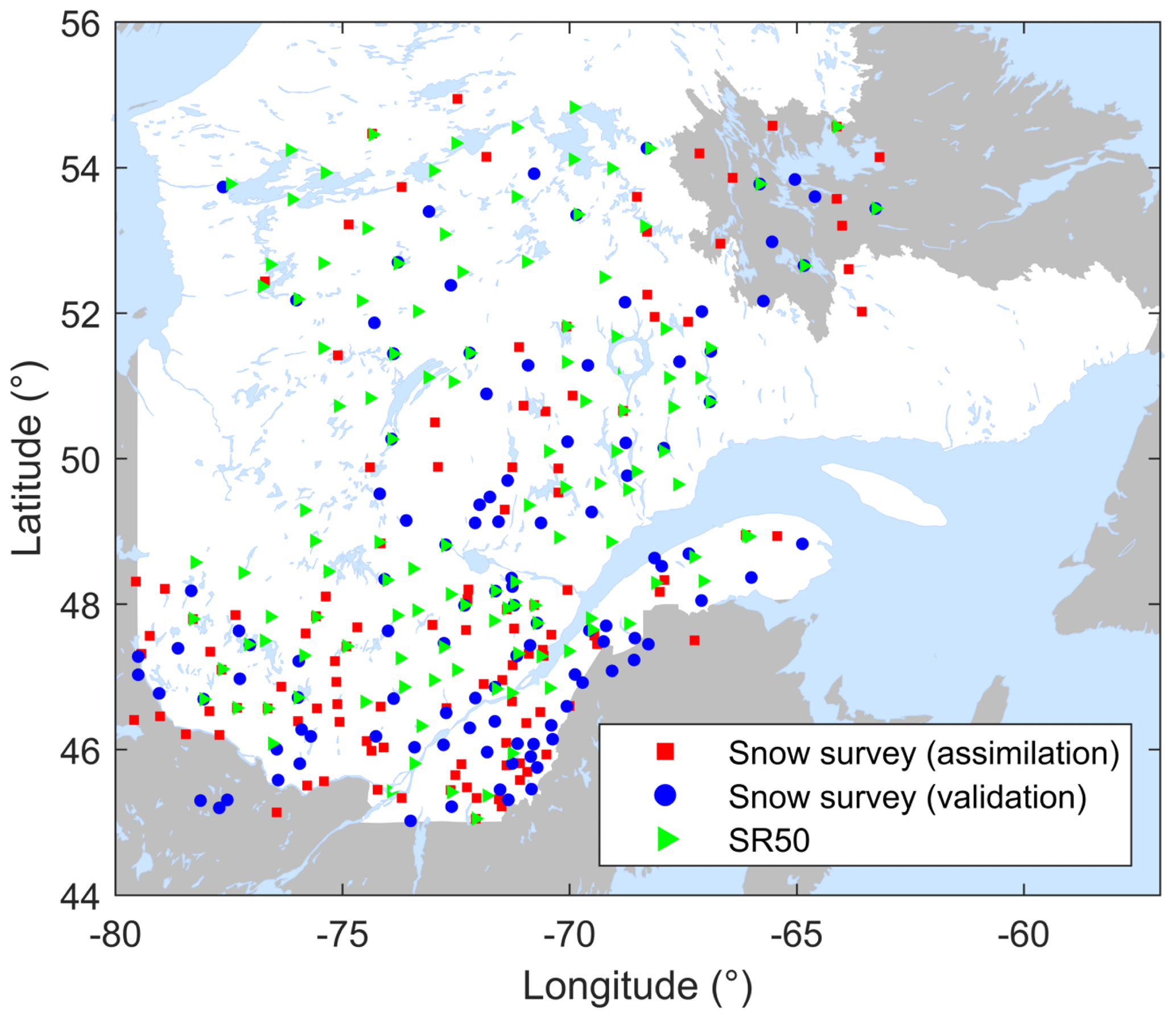
Figure 1 Snow observation sites in and around Quebec (Canada).

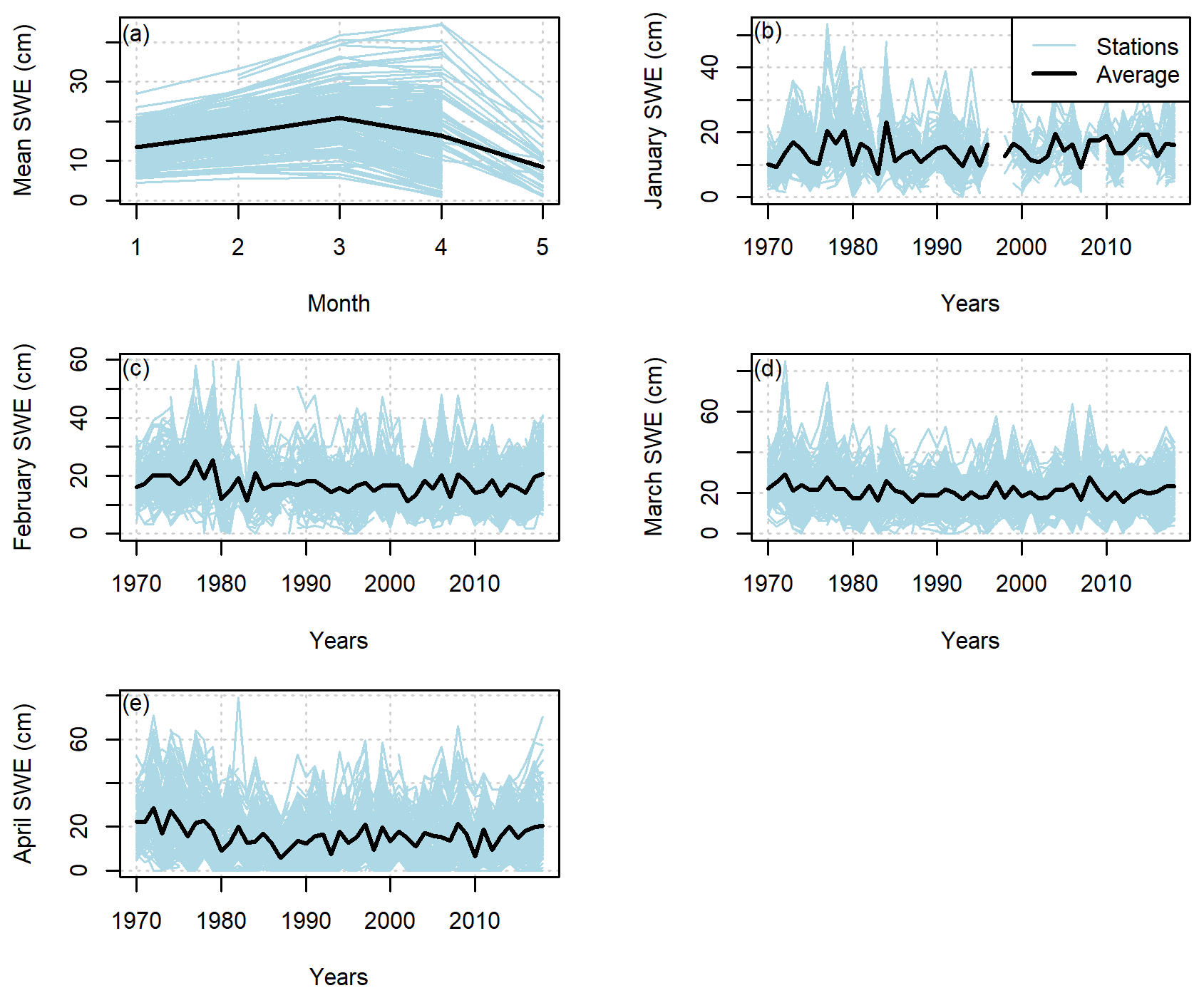
Figure 2 Averaged SWE observations in the study area between 1961 and 2018 (a) over the entire year, (b) in January, (c) in February, (d) in March and (e) in April.

This research focuses on a portion of the province located south of 53^∘ N, where most of the population is concentrated. Northern Quebec differs markedly from the more southern region in terms of the amount of available snow data and snow characteristics; therefore, its inclusion would require a separate study.

2.2 Snow model and meteorological forcing

We use the HYDROTEL snowpack model (HSM) in this study (Turcotte et al., 2007), which is used operationally for real-time SWE estimation at the MELCC. HSM is a temperature-index-based model and therefore provides a simplified representation of the water and energy budgets of the snowpack. It is a rather simple snow model that only requires daily precipitation and minimum and maximum temperatures as inputs. The implementation and parameterization of the model are those proposed by Cantet et al. (2019). More detailed specifications about the model structure and physics can be found in Turcotte et al. (2007).

To force the HSM, daily grids of precipitation and minimum and maximum temperatures are used. They are produced by the MELCC by kriging in situ measurements from local meteorological ground stations (Bergeron, 2015) on a regular 0.1^∘ resolution grid. Along with the interpolated variables, the corresponding kriging variances are also produced. They cover the entire 1961–2018 period.

3 Methodology

3.1 Spatialized particle filter

The particle filter implemented in this study is the one developed and tested by Cantet et al. (2019). This method was developed to assimilate at-site snow data into a large-scale modelling framework. The main feature is to generate particles characterized by a realistic temporal and spatial correlation so that each particle can be seen as a reasonable scenario. The observations are then used to weight the different particles when and where they are available. In this context, it is hypothesized that the weights should be spatially correlated, given that the particles are also spatially correlated. In a second step, the weights estimated at observation sites are interpolated in space. To avoid filter degeneracy, Cantet et al. (2019) implemented the sampling importance resampling algorithm from Gordon et al. (1993).

The spatialized particle filter proposed by Cantet et al. (2019) differs from more traditional approaches such as the ones described by Farchi and Bocquet (2018). In Cantet et al. (2019), the likelihood of the particles is evaluated locally at each observation site. The likelihood is then multiplied by the prior weights to derive the posterior weights. The posterior weights at observation sites are then interpolated in space. In the traditional localized approach, the likelihood is evaluated over a certain area (a block or radius around an observation), and the posterior weights are directly derived for this area by multiplying the prior by the likelihood. However, the interpolation step in the approach of Cantet et al. (2019) could tend to make it less selective and to keep a particle as long as an observation provides it with a sufficiently high weight.

Following Cantet et al. (2019), we generated 500 particles using perturbations of the meteorological input data and the predicted SWE. Perturbations of the precipitation and temperature inputs should represent the uncertainty associated with the forcing. Given that these inputs are created through a spatial interpolation, they are perturbed using an additive noise following Gaussian distribution for which the variance is set to the interpolation variance. The simulated SWE is perturbed with a multiplicative uniform noise proposed by Clark et al. (2008) and used in Leisenring and Moradkhani (2011); this perturbation process represents the structural uncertainty associated with the snow model. The temporal correlation of the noise is maintained using the formulation (Evensen, 1994)

$$\begin{array}{}\text{(1)}& s_t=\mathit{\alpha }{s}_{t-\mathrm{1}}+\sqrt{\mathrm{1}-{\mathit{\alpha }}^{\mathrm{2}}}{\mathit{\eta }}_t,\text{with}{s}_{\mathrm{0}}\sim \mathcal{N}(\mathrm{0},\mathrm{1}),\end{array}$$

where s_t is the random noise at time t, α represents the temporal correlation and is set at 0.95, and η_t is a random white noise following a standard normal distribution.

The spatial correlation of the noise is built up using the exponential model (Uboldi et al., 2008)

$$\begin{array}{}\text{(2)}& r=\exp {\displaystyle \frac{-d^{\mathrm{2}}}{L^{\mathrm{2}}}},\end{array}$$

where r is the spatial correlation between two points separated by a distance d, and L is the range of the correlation, set at 200 km (Cantet et al., 2019).

In our study, local particle filters are implemented at the observation sites. The weight of a given particle at an observation site at a specific time when an observation is available depends on the likelihood of the measured SWE value given the SWE associated with this particle. This likelihood is represented by a Gaussian process:

$$\begin{array}{}\text{(3)}& y_t|x_t^i\sim \mathcal{N}(y_t-x_t^i,{\mathit{\sigma }}^{\mathrm{2}}),\end{array}$$

where y_t represents the observed SWE at time t, $x_t^i$ is the SWE simulated by the ith particle, and σ is the standard deviation of the Gaussian process, which is related to the uncertainty associated with each type of SWE observation and is expressed in SWE units. For manual snow surveys, σ should represent both the uncertainty of the measurement itself and the error of the spatial representativeness, i.e. how well a local measurement can represent the SWE averaged over a grid cell. σ is tuned to $a\times (\mathrm{0.1}\times y_t+\mathrm{1})$, where a is a unitless parameter set at 3 for the snow survey observations (by trial and error by Cantet et al., 2019) and is to be determined for the SR50. In the case of the SWE estimated from the SR50 snow depth measurements, σ should also represent the structural uncertainty of the artificial neural network model (Odry et al., 2020) used to estimate SWE. Moreover, although manual snow surveys average 10 measurements along a 100–300 m snow line, SR50 sensors provide a purely at-point measurement. As a consequence, the error for the spatial representativeness should be larger for SR50 than for manual snow surveys.

Under these assumptions, when a given observation becomes available at time t, the weight $x_t^i$ associated with the ith particle at the observation site can be updated to

$$\begin{array}{}\text{(4)}& w_t^i={\displaystyle \frac{w_{t-\mathrm{1}}^{i}p\left(y_t\right|x_t^i)}{\sum _{i=\mathrm{1}}^{N_{\mathrm{P}}}{w}_{t-\mathrm{1}}^{i}p\left(y_t\right|x_t^i)}},\end{array}$$

where N_P is the number of particles. One can notice that the weight of a particle at a given time step depends on the weight at the previous time step. Therefore, the assimilation of continuous data with a time correlation can lead to the assimilation of the same information several times and can cause too much weight to be given to this information. Here, it is chosen that the SR50 should be assimilated at a weekly frequency. In operational real-time simulations, the model is restarted each day from 7 days in the past to include all observations obtained over that 1-week period. It would thus be possible to assimilate only the most recent SR50 observation and have an assimilation frequency of close to weekly.

At a given time step, the weights are updated for any newly available observation using Eq. (4). The weights at the observation sites are spatially interpolated using a simple inverse distance-weighted method to estimate the weights for each grid cell. This process makes it possible to include different observations obtained inside the same grid cell.

Once the weights have been updated and interpolated, it is possible to investigate the risk of filter degeneracy. Degeneracy occurs when a few particles concentrate all the weight. For each observation site and grid cell, $N_t^{\mathrm{eff}}$, the effective sample size at time t, is computed as

$$\begin{array}{}\text{(5)}& N_t^{\mathrm{eff}}={\displaystyle \frac{\mathrm{1}}{\sum _{i=\mathrm{1}}^{N_{\mathrm{P}}}(w_t^i{)}^{\mathrm{2}}}}.\end{array}$$

If the effective sample size falls below the 0.8N_P threshold (Magnusson et al., 2017), the particles are then locally resampled. It is important to highlight that whereas the particles are generated with a spatial structure, they are evaluated and resampled locally. The resampling is performed using the SIR algorithm (Gordon et al., 1993) and consists of deleting the particles with the lowest weights and duplicating those with the largest weights. The objective of this resampling is to obtain a set of particles associated with equal weights of $\frac{\mathrm{1}}{N_{\mathrm{P}}}$ that describe the same distribution as the weighted particles before resampling. Through this process, the filter retains a large number of meaningful particles while the posterior distribution of SWE is marginally affected (the resampling algorithm should be selected to limit the impact on the posterior distribution). Moreover, the SWE values and other state variables of the different particles are not modified.

Although the resampling aims to preserve the filter from degeneracy, it is also responsible for the risk of spatial discontinuity, as it is performed independently for each site and grid cell. The risk of discontinuity is managed using a reordering of the particles.

3.2 Recovering the spatial structure by reordering the particles

We implemented two alternative procedures to maintain the spatial structure of each particle despite resampling: the Schaake shuffle, proposed by Clark et al. (2004), and a simple sorting of the particles at each site. The use of any of these strategies in the context of particle filtering constitutes the novelty of this piece of research.

The Schaake shuffle is a reordering method that aims to recover the space–time structure in an ensemble of precipitation or temperature forecast fields. In the original application of the Schaake shuffle, the spatial structure of the ensemble members is lost during a downscaling procedure. The idea behind the Schaake shuffle is to rank the members of the ensemble and match these ranks with those of past observations selected randomly from similar dates in the historical records. Although the Schaake shuffle was not initially developed to be applied to the field of snow or data assimilation, there is no technical difficulty in transferring its application from an ensemble of meteorological forecasts to a set of particles describing a snowpack.

For a given time and location, let X be the vector (of length N_P) of SWE values for all the particles. A vector of equal size Y is built from the historical record at the same location and a similar date. Considerations about the construction of Y are provided in the following sections. The vectors χ and γ are the sorted versions of X and Y, respectively:

$$\begin{array}{}\text{(6)}& {\displaystyle }\mathit{X}=(x_{\mathrm{1}},x_{\mathrm{2}},\mathrm{\dots },x_{N_{\mathrm{P}}}),\text{(7)}& {\displaystyle }\mathit{\chi }=(x_{\left(\mathrm{1}\right)},x_{\left(\mathrm{2}\right)},\mathrm{\dots },x_{\left(N_{\mathrm{P}}\right)}),\text{where}{x}_{\left(\mathrm{1}\right)}\le x_{\left(\mathrm{2}\right)}\le \mathrm{\dots }\le x_{\left(N_{\mathrm{P}}\right)},\text{(8)}& {\displaystyle }\mathit{Y}=(y_{\mathrm{1}},y_{\mathrm{2}},\mathrm{\dots },y_{N_{\mathrm{P}}}),\text{(9)}& {\displaystyle }\mathit{\gamma }=(y_{\left(\mathrm{1}\right)},y_{\left(\mathrm{2}\right)},\mathrm{\dots },y_{\left(N_{\mathrm{P}}\right)}),\text{where}{y}_{\left(\mathrm{1}\right)}\le y_{\left(\mathrm{2}\right)}\le \mathrm{\dots }\le y_{\left(N_{\mathrm{P}}\right)}.\end{array}$$

Moreover, B is taken as the vector of indices describing the positions of the elements of γ in the original vector Y. That is to say, the ith element of B describes where to find the ith element of γ in Y. Finally, if Z is the reordered version of X, then

$$\begin{array}{}\text{(10)}& \mathit{Z}=(z_{\mathrm{1}},z_{\mathrm{2}},\mathrm{\dots },z_{N_{\mathrm{P}}}),\end{array}$$

with

$$\begin{array}{}\text{(11)}& {\displaystyle }{z}_q=x_{\left(r\right)},\text{(12)}& {\displaystyle }q=\mathit{B}\left[r\right],\end{array}$$

and

$$\begin{array}{}\text{(13)}& r=\mathrm{1},\mathrm{\dots },N_{\mathrm{P}}.\end{array}$$

This reordering must be applied at each site or grid cell. A more detailed procedure and a visual example are provided in (Clark et al., 2004).

As it appears in Eqs. (7)–(13), the main limitation to the application of the Schaake shuffle is the availability of historical records for the construction of vector Y. It is necessary to have records covering each site (observation sites and grid cells) and for them to be of sufficient length to be able to draw N_P values from similar periods for each site. Given that an extensive data set does not exist for the SWE in Quebec, we propose to use a record of simulations made using the HSM in its deterministic configuration without assimilation. This selection relies on the assumption that the model without data assimilation can correctly estimate the spatial structure of the SWE. This is a fairly strong assumption; nevertheless, in the absence of a spatially distributed SWE product covering the whole study area for a long period of time, and considering that the spatial structure in the HSM deterministic simulation is controlled by the meteorological inputs and not a pre-imposed spatial structure, this choice is considered reasonable. One can notice that the actual SWE values in the historical records are not used in the Schaake shuffle; only their respective rank is used to reorder the particles, so the estimation errors and biases from the model are not of prime importance. In our application, the vector Y is constructed from a reference set of simulations produced with a deterministic run of the HSM for the years 1961 to 2004. It is assumed that the overall spatial structure of the SWE remains the same during this period. This assumption is difficult to verify as there is no spatial observation of the SWE covering the whole area and period, but Fig. 2 does not show any strong tendency over the period. Following Clark et al. (2004), only values associated with a date within a window of ±7 d around the assimilation date (but with different years) are used. The vector Y is built by randomly drawing 500 values from the 660 available records.

As a simpler alternative to the Schaake shuffle, we also implemented a sorting of the particles. In this case, at each site, all 500 particles are sorted in ascending order of SWE value. The idea is to rebuild the correlation between the sets of particles in neighbouring sites in the sense of the rank correlation. Although the sorting procedure is much simpler to implement and does not require any reference record, it also removes the possibility to consider each particle as a reasonable snow scenario at a large scale. Compared to the Schaake shuffle, the sorting can be seen as a way of trading the large-scale structure for a short-scale one.

3.3 Validation procedure and metrics

To evaluate the impacts of the different reordering strategies on the spatial structure of the particles and the final SWE estimation, we use experimental variograms. These plots provide the evolution of the variance between the sites as a function of the separation distance. Because the variograms are only computed for a single date, the Pearson correlation between the 500 SWE values (from each particle) at two nearby sites is also used and computed at each time step so that the temporal evolution of the spatial structure can also be assessed. When investigating the spatial structure, all snow survey sites are used for assimilation.

To assess the ability of the overall method to estimate the SWE, we compute two deterministic scores, the root mean squared error (RMSE) and the mean bias error (MBE), as well as two ensemble-based scores: the continuous ranked probability score (CRPS, Matheson and Winkler, 1976) and the skill-to-spread ratio (Fortin et al., 2014). The CRPS considers two, sometimes competing, aspects of ensemble quality. The first aspect is resolution. An ensemble has a good resolution (or sharpness) when it discriminates events. For instance, a climatological ensemble that covers the whole range of possibilities has no resolution. A deterministic simulation series that follows the observed series very closely has an excellent resolution. The second aspect is reliability. Reliable ensembles display exactly the right amount of variability. For instance, a 95 % confidence interval computed from the daily ensemble is reliable if it contains the observation 95 % of the time on average. The RMSE is a measure of accuracy, which is related to the resolution. If two different series of ensemble simulations have the same level of resolution (similar RMSEs) but very different reliability values, the more reliable one will obtain a lower (better) CRPS.

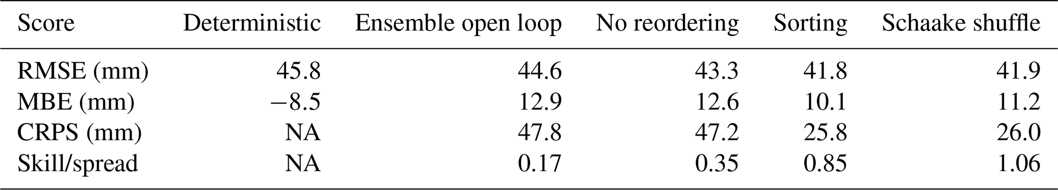
The metrics are summarized in Table 1. As the purpose of the spatialized particle filter is mainly to produce estimates at ungauged sites, only 50 % of the manual snow survey sites are used for the assimilation; the other half are kept as a validation subset. This sub-sampling strategy is presented in Fig. 1. All provided scores are computed only on the validation subset.

Table 1 Performance metrics.

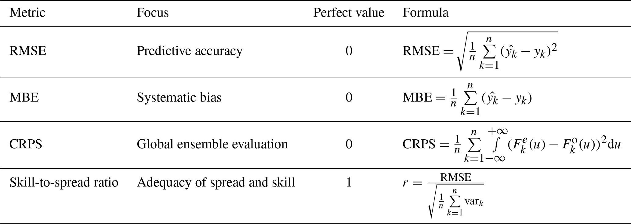
n is the number of points, x_k and $\widehat{x_k}$ are respectively the estimated and observed SWE values, var_k is the variance of the particles of the kth point, $F_k^e$ is the cumulative distribution function described by the weighted particles of the kth point, and $F_k^{\mathrm{o}}$ is the Heaviside function associated with the observation.

4 Results and discussion

4.1 Spatial structure of the particles

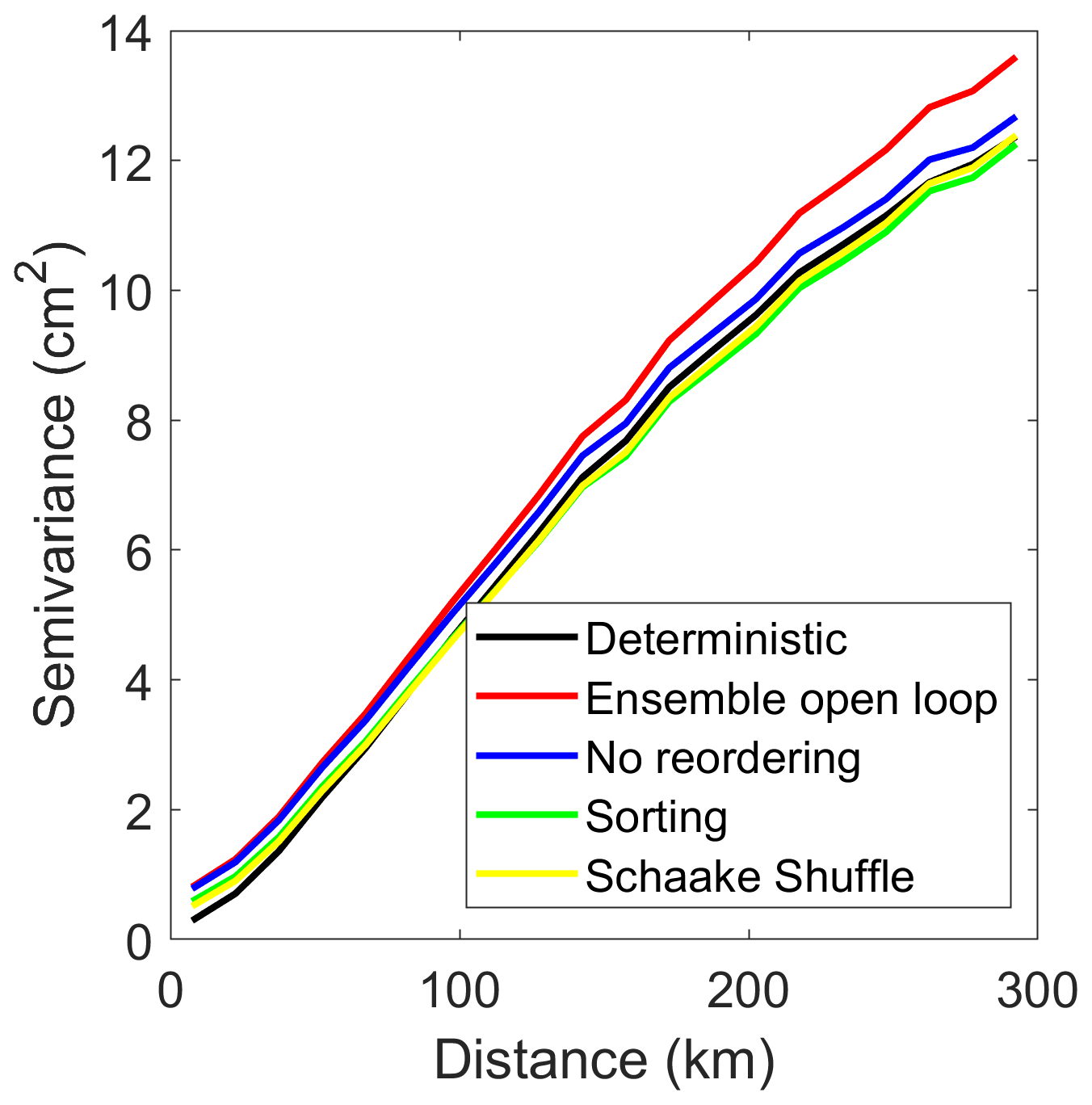
The variograms of the estimated SWE for 28 February 2012, for the different configurations (deterministic run, ensemble open loop, assimilation without reordering, assimilation with sorting of the particles, and assimilation with the Schaake shuffle) are provided in Fig. 3. We selected 28 February because February is considered to be the last month of the accumulation season in Quebec. The deterministic run corresponds to the deterministic simulation of the HSM without any assimilation, whereas the three other curves correspond to the weighted average of the 500 particles. The five variograms are very similar, which demonstrates that the different assimilation strategies lead to final SWE estimates that are comparable to the deterministic run of the HSM, with similar spatial structures. This similarity is a desired behavior, as the spatial structure should be guided by the snow model and its meteorological forcings. In particular, Fig. 3 demonstrates that particle reordering does not affect the overall spatial structure of the final SWE estimate.

The variograms in Fig. 3 have a semi-variance of below 1 cm² for separation distances close to 0. The semi-variance that corresponds to a null distance (also called the nugget effect) is important, as it describes the spatial roughness or local noise. The presence of spatial discontinuities would create a noticeable nugget effect. As expected, the deterministic model is characterized by the lowest nugget effect (around 0 cm²), which means an absence of local random noise. In addition, it is interesting to note that the assimilation without reordering has the largest nugget effect, with a value around 1 cm². This large nugget effect can be a symptom of some noise affecting the correlation between neighbouring sites. Finally, the ensemble open loop displays the largest long-distance semi-variance, which is a result of a larger dispersion of the particles. This is expected in the absence of data assimilation. Despite those small differences, we conclude that the different configurations result in comparable spatial structures.

Figure 3 Variograms of the estimated snow water equivalent (SWE) on 28 February 2012.

The maps corresponding to the variograms in Fig. 3 are provided in Fig. 4. The five maps exhibit a similar spatial pattern, although the map from the deterministic simulation (panel a) is the most distinct from the other ones. This was expected because no assimilation is involved in this simulation. The deterministic simulation also provides a smoother map compared with the other three, which is compatible with what is observed in the variograms. The overall similarity of the different maps was expected, considering that they are characterized by similar variograms. Figure 4 evidences that the assimilation process as well as the different reordering methods do not impact the spatial structure of the final SWE estimate. This behaviour was expected, since the overall structure is driven by the forcing data and the spatially correlated perturbations. Figure 4 shows that the reordering process does not affect the overall spatial structure of the estimated SWE.

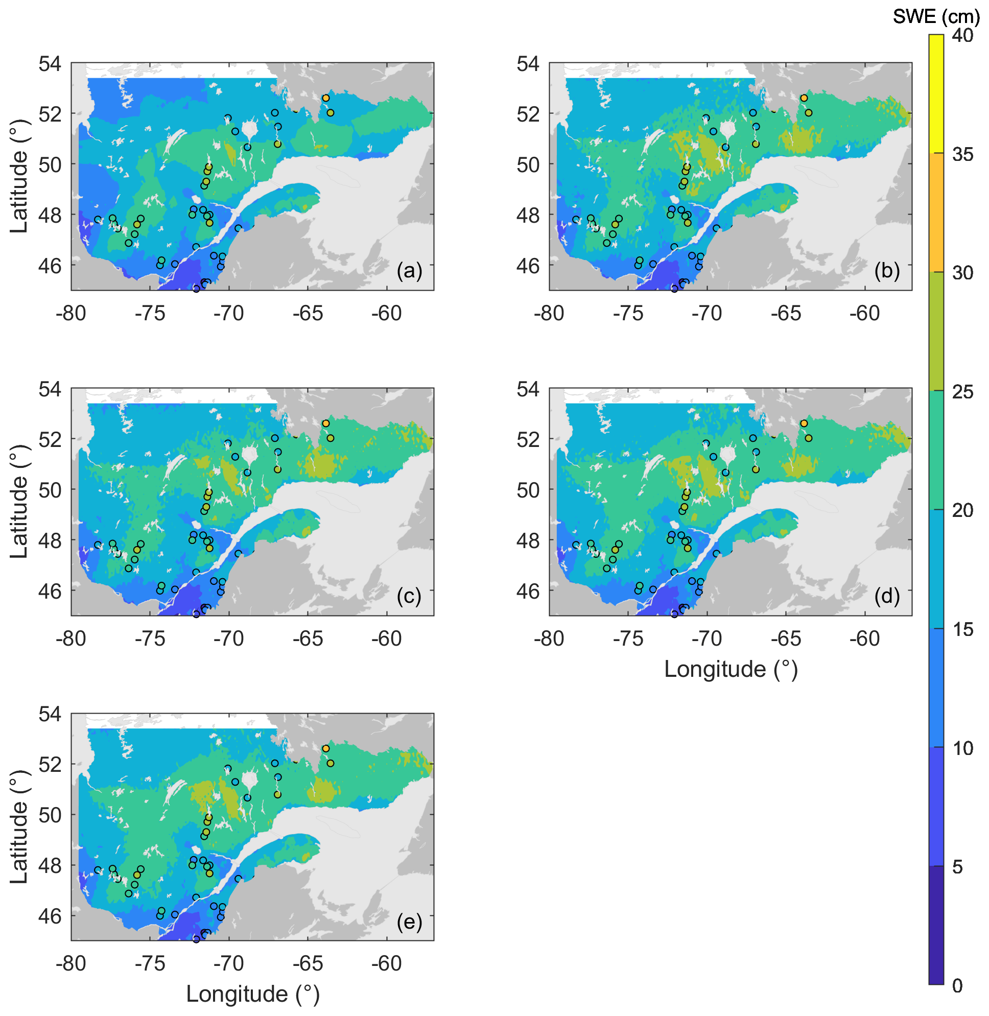
Figure 4 Estimated snow water equivalent (SWE) maps for 28 February 2012: (a) deterministic run, (b) ensemble open loop, (c) no reordering, (d) sorting and (e) Schaake shuffle; points represent the locations of the available snow surveys on this day.

Nevertheless, although it is important to assess the spatial structure of the final SWE estimates, the spatialized particle filter relies on the assumption that the weights of the particles can be interpolated in space. Therefore, the spatial structure of each particle must be preserved. To verify this, we plotted the variograms of the 500 particles for the three reordering options: no reordering, sorting the particles in ascending order and the Schaake shuffle (Fig. 5). In Fig. 5, the thin grey curves represent the variograms of individual particles, whereas the bold coloured lines are identical to those in Fig. 3. Note that the vertical axes do not share the same scale. Moreover, the maps corresponding to two particles (number 250 and number 500) are provided in Fig. 6 to illustrate the link between the variograms and the overall spatial structure. First, for both the ensemble open loop and the assimilation without reordering (Fig. 5a and b), it is clear that the individual spatial structure of each particle is different from the weighted average. More specifically, all particles are characterized by a much larger nugget effect, ranging from approximately 100 to around 600 cm². Therefore, there is significant short-range random variability. This nugget effect can also be observed in Fig. 6a and b as well as c and d, where the maps display a very granular aspect. The fact that individual particles exhibit an important nugget effect whereas their weighted average does not exhibit this effect indicates that a large amount of random noise is associated with each particle, which is in disagreement with the underlying assumptions of the spatialized particle filter.

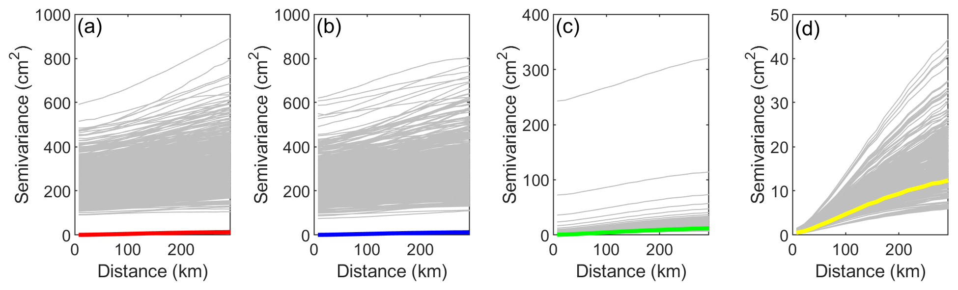
Figure 5 Variograms of the particles for the different reordering strategies for 28 February 2012: (a) ensemble open loop; (b) no reordering, (c) sorting and (d) Schaake shuffle. Solid lines represent the variograms of the estimated SWE as displayed in Fig. 3, and grey lines represent the variograms of individual particles.

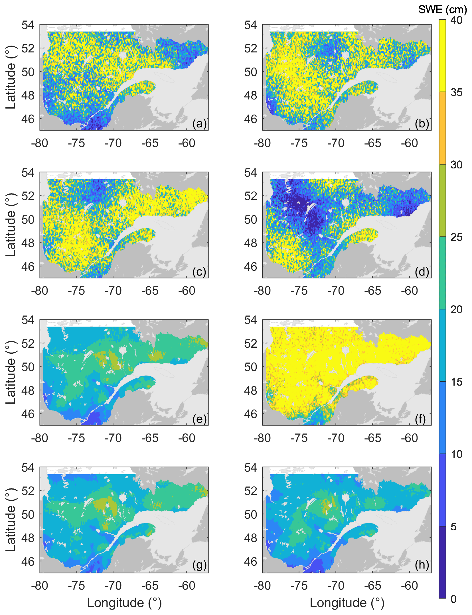
Figure 6 Snow water equivalent (SWE) for two particles on 28 February 2012: particle #250 (a, c, e, g) and particle #500 (b, d, f, h); ensemble open loop (a, b), no reordering (c, d), sorting (e, f) and Schaake shuffle (g, h).

Figure 5c shows the variograms of the individual particles when the particles are sorted in ascending order following each resampling. This sorting attenuates the random noise associated with individual particles very effectively. Following this sorting, most particles fall around the final estimate. Nevertheless, some still exhibit a very large nugget effect. This granularity is associated with the accumulation of small random differences between neighbouring cells throughout the winter. Even though the perturbations (in precipitation, temperature and SWE) are spatially correlated, they are not perfectly identical. This nugget effect on individual particles dissipates when the particles are averaged, as seen in Figs. 3, 4 and 5. Upon reordering the particles in ascending order, we expected that some of those particles would display a disturbed spatial structure. Panels e and f of Fig. 6 provide more insight regarding this expectation. The maps represent the states of two individual particles (#250 and #500) for a given moment in time. The two particles present very different patterns. This difference was expected, as particle #250 is located in the middle of the ensemble, whereas particle #500 gathers all the highest SWE values. Such differences illustrate that when particles are sorted in ascending order, the individual particles cannot be considered potential SWE map scenarios anymore. Sorting can rebuild the short-range correlation, which is necessary overall for the spatialized particle filter, but that same sorting can jeopardize the long-range correlation and the general spatial pattern.

Reordering the particles with the Schaake shuffle appears to be a better option to fix the spatial structure of the particles. Figure 5d illustrates that all particles have a near-zero nugget effect, and their variograms lie around that of the final estimate. This is compatible with the idea that the particles are alternative SWE scenarios, each providing a reasonable spatial structure. The same conclusions can be drawn from Fig. 6h and g.

As a summary, Figs. 5 and 6 demonstrate that the individual particles are characterized by a nonrealistic spatial structure in the ensemble open loop and when the assimilation is performed without any reordering. In both cases, the particles are characterized a strong nugget effect, which is also associated with granular SWE maps. This behaviour is incompatible with the underlying assumptions of the spatialized particle filter. On the contrary, the two reordering methods result in more realistic spatial structures for the individual particles. However, simply sorting the particles in ascending order produces some problematic particles. Only the Schaake shuffle is able to maintain an acceptable spatial structure for all individual particles.

To evidence the temporal evolution of the spatial structure, we refer to Fig. 7, which shows the evolution of the correlation coefficient between the sets of particles at two given neighbouring sites for winter 2011–2012. In this figure, the vertical dotted lines represent assimilation dates. Due to the proximity of the two sites, a strong correlation between both sets of particles is to be expected, as the SWE is correlated in space at a short distance in reality.

Figure 7 also shows the results for data assimilation without any resampling, in order to assess the impact of resampling on the spatial structure. Correlation decreases continuously with time for the assimilation without resampling (nor reordering) and without reordering. The main difference between those two options is a sudden drop in correlation values in late February for the case of resampling without reordering. This drop is associated with a resampling. Whereas resampling can be associated with a large and immediate drop in correlation because of a disassociation of particles at different sites, resampling cannot explain the continuous decrease in correlation. This decrease can be explained, however, by the cumulative nature of the snowpack and the perturbations. In this study and following Cantet et al. (2019), precipitation, temperature and SWE itself are perturbed independently. The perturbations are generated with a spatial structure, meaning that perturbations applied to neighbouring sites are strongly correlated but are not identical. The simulated snowpack accumulates these differences throughout the winter, thus explaining the continuous decrease in correlation. Therefore, it appears that the assumption used to justify the interpolation of particle weights is not supported after a certain number of time steps without reordering, and resampling only aggravates the problem.

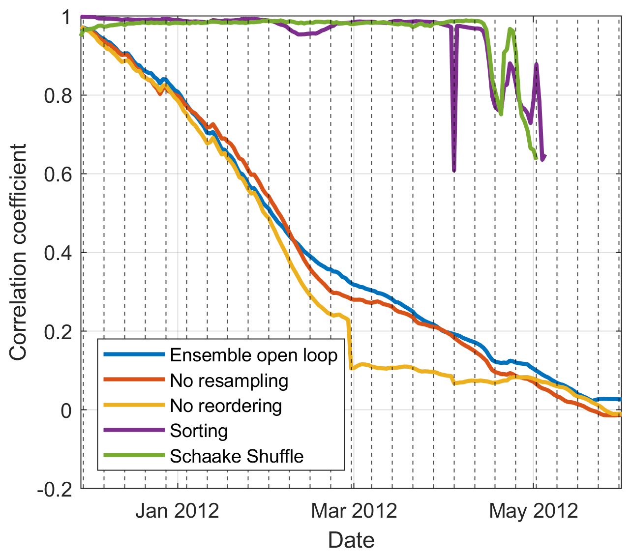
Figure 7 Evolution of the correlation between between two adjacent grid cells over the winter of 2011–2012.

In Fig. 7, the two reordering strategies maintain a very high correlation between neighbouring sites. Some momentary correlation losses are observed in April, which can be associated with the disappearing snow (some grid cells and particles have no snow).

As a consequence, it appears that both reordering strategies can maintain the spatial structure of the particles. In the present context, such reordering is necessary to verify the underlying assumption of the spatial particle filter and to ensure that the weights of the particles can be interpolated meaningfully. From a more general point of view, reordering the particles appears to be an effective way to deal with the spatial discontinuities created by the resampling step of the particle filter. Reordering by sorting the particles in ascending order is easy to implement, as it does not require any additional data set, but in this case, the individual particles cannot be seen as scenarios that each have a reasonable long-range correlation. In contrast, the Schaake shuffle preserves the idea of each particle representing a potential realistic scenario. Consequently, because the spatialized particle filter relies largely on spatially structured perturbations and particles, the Schaake shuffle appears to be a better solution. Nonetheless, the Schaake shuffle requires a long spatialized record to build the reference set. Here, we demonstrate that a simulated deterministic run can be used as a pseudo-historic climatology of SWE if we assume that the model can simulate a realistic spatial structure. Still, in situations where a reference set cannot be acquired or created, reordering particles by sorting them in ascending order can be an acceptable alternative to maintain the short-range correlation of the particles.

4.2 Snow water equivalent estimation

In this and the following sections, all scores are computed solely on the validation subset (see Fig. 1); the SWE data from the validation sites are never assimilated. The calculated scores are intended to show the ability of the spatialized PF to estimate SWE in ungauged sites.

Figure 8 presents the cumulative distributions of the different performance metrics over the validation sites when only manual snow surveys are assimilated. Table 2 provides the scores averaged over all the sites in the validation sample. The shift from the deterministic to the ensemble open-loop configuration as well as the data assimilation noticeably reduce the RMSE (panel a) and the MBE (panel b) relative to the deterministic run simulation. The ensemble open-loop simulation is characterized by as much bias as the simulations with data assimilation, but the ensemble open-loop simulation obtains a higher (worse) RMSE. Nonetheless, the three assimilation and reordering strategies show comparable values of RMSE and MBE. There seems to be only a slight decrease in RMSE when using the Schaake shuffle. Differences are more noticeable for ensemble-based performance metrics. First and foremost, Fig. 8c exhibits a large decrease in CRPS when using one of the reordering methods. As the RMSE values are comparable, this improvement of the CRPS is necessarily associated with a narrowing of the posterior distribution described by the particles. This result can be linked with the reduced amount of random noise associated with the reordering of the particles (see Sect. 4.1). A reduction in ensemble spread is also apparent in Fig. 8d. Because the skill (evaluated using the RMSE) is not sensitive to the reordering, the increase in the skill-to-spread ratio can only be explained by a reduction of the spread. The ratio is also systematically higher with the Schaake shuffle than with the sorting, meaning that the Schaake shuffle makes the spread of the ensemble of particles even narrower. In the case of simple sorting, 80 % of the sites have a ratio below 1; thus, the particles are over-dispersive. The situation improves slightly with the use of the Schaake shuffle. As expected, the ensemble open-loop simulation is characterized by the worst ensemble scores. In the absence of assimilation, the particles are free to evolve, and the dispersion of the ensemble becomes very large.

Figure 8 shows that the gain in deterministic error reduction from particle reordering is very limited. Nevertheless, reordering the particles greatly improves the ensemble scores, which means that the posterior distribution of the particles is a better estimate of the actual uncertainty. Considering that data assimilation techniques in hydrology are mainly used for forecast applications, better quantification of the uncertainty is a very important achievement. According to those results, the simple sorting of the particles appears to be as effective as the more elaborate Schaake shuffle at maintaining the spatial structure of the particles.

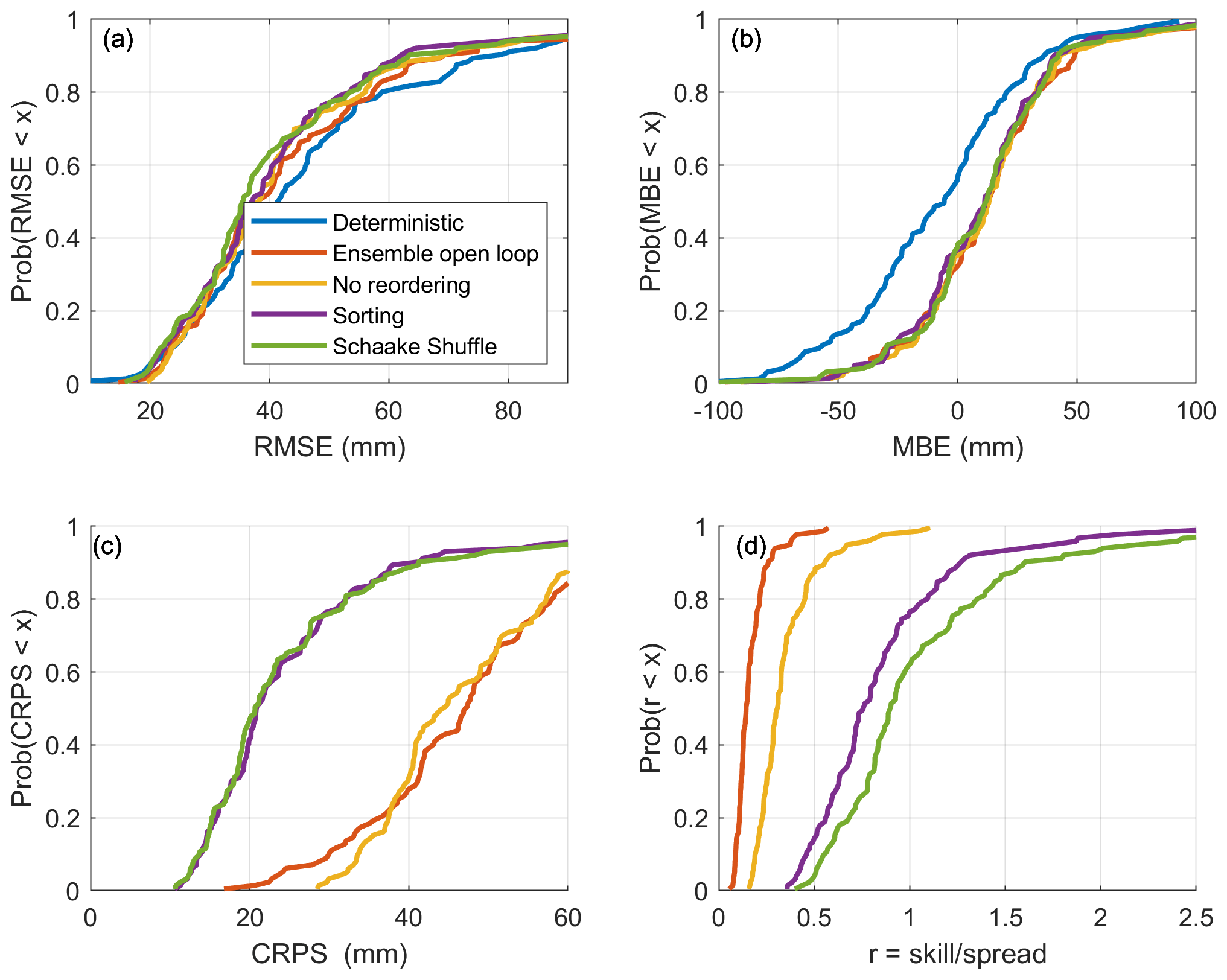
Figure 8 Cumulative distributions of the scores calculated for the 50 % validation snow courses.

Table 2 Scores averaged over the 50 % validation snow courses.

4.3 Inclusion of the data from the SR50 sensors within the assimilation scheme

The inclusion of the data from SR50 sensors in the experiment aims at improving the spatio-temporal coverage of the territory in terms of observations. This new dataset includes new observation sites and continuous time series. The first step before including the SR50 data is to estimate the uncertainty associated with the indirect observations. The total uncertainty is composed of the measurement uncertainty, the depth-to-SWE conversion error, and the spatial representativeness error. Here, the spatial representativeness error represents the difference between the local in situ observation and the simulated value, which is averaged over a 0.1^∘ resolution grid cell.

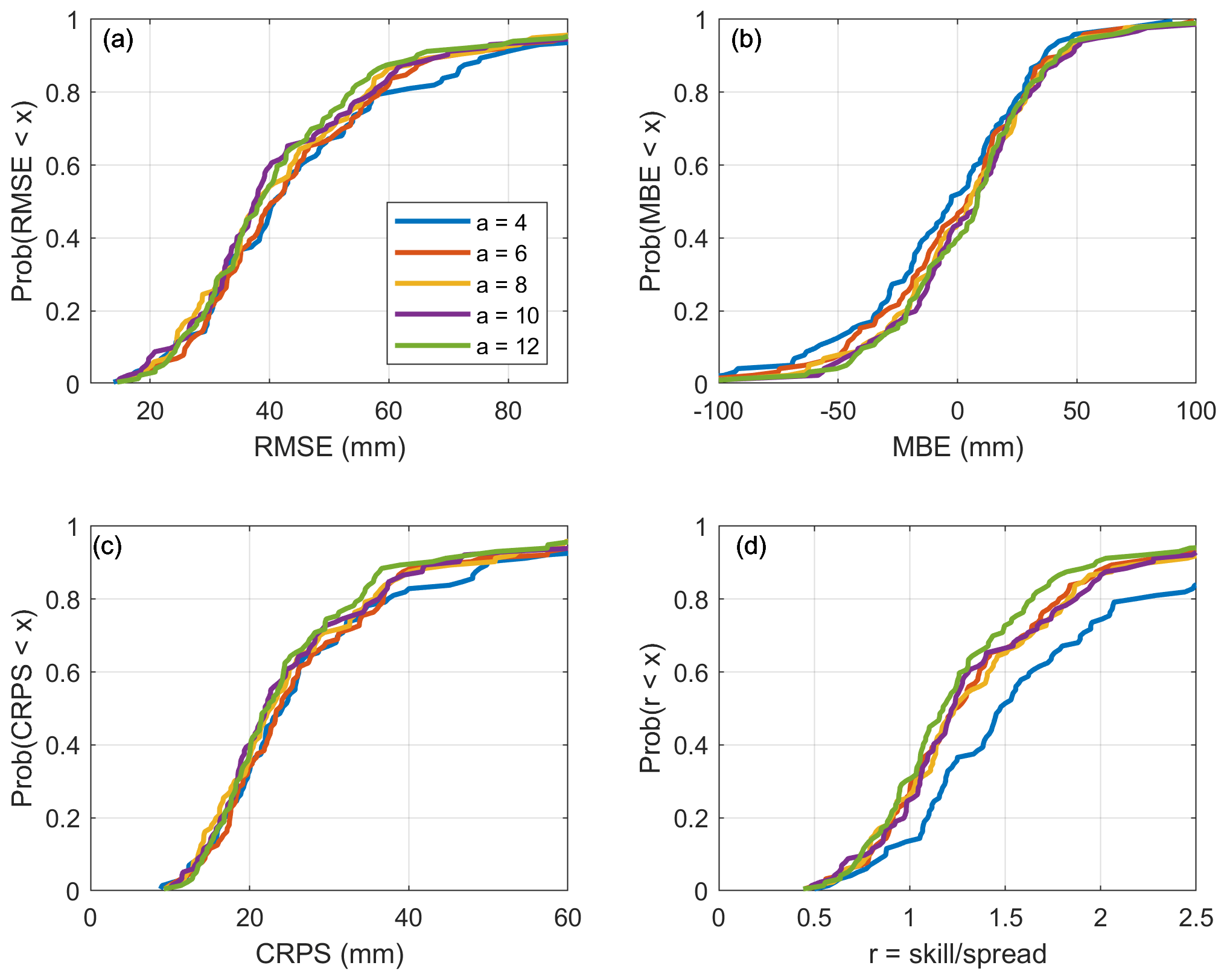
Figure 9 Cumulative distributions of the scores for the validation sites when assimilating SR50 data, according to the applied uncertainty model.

We assume that the uncertainty associated with the SR50 data follows the specifications provided in Sect. 3.1. Figure 9 displays the cumulative distributions of the performance metrics at validation sites when only the SR50 data are assimilated for different a values. The first observation is that the lowest (worst) scores are achieved for an a value of 4. Higher (better) scores are attained at higher a values, which confirms that the uncertainty associated with the SR50 must be greater than that of the snow surveys. It also appears that if a is greater than 4, there are no large differences in the distributions of RMSE, MBE or CRPS. Thus, the performance is not very sensitive to the a value as long as this is sufficiently high (greater than 4). In Fig. 9d, the skill-to-spread ratio increases with the a value of the uncertainty associated with the SR50 observations. This result indicates that greater uncertainty for these observations creates a larger spread of the particles, which is expected, as a higher observation uncertainty provides greater flexibility to the particles around the observation and gives more weight to the prior distribution. Here, in the end, and considering the observations above, we selected an a value of 10 for the SR50 data as a reasonable compromise.

Figure 10 displays the cumulative distributions of the performance metrics over the validation sites according to the type of data that is assimilated: snow surveys only, SR50 only, or both. First, all assimilation schemes significantly reduce the RMSE (panel a) for most sites compared to the deterministic run. These results, similar to those of Cantet et al. (2019), demonstrate that the spatialized particle filter can assimilate local observations and use them to improve the global estimation of SWE. In panel b, the assimilation schemes increase the MBE values at all sites relative to those of the deterministic simulation, which confirms that assimilation tends to correct the underestimation of the deterministic simulation. When comparing the dependence of the RMSE (panel a) and that of the CRPS (panel c) on the type of data that are assimilated, improved results are obtained when only the snow surveys are assimilated. The assimilation of SR50 observations only or both types of observations simultaneously yields comparable performance, although it is still higher (better) than that of the deterministic run. Thus, in the absence of snow surveys, it is possible and even desirable to assimilate estimated SWE data from SR50 observations to improve the simulation of SWE. Nonetheless, at this point, the validation process reaches its limitations. In our study, 50 % of the snow survey sites are used in validation; therefore, it is assumed that these observations represent the actual amount of SWE. Nevertheless, the model simulates the SWE over a grid having a 0.1^∘ resolution, so local observations may not be representative. Moreover, SR50 sensors and snow survey sites tend not to be installed in the same environment; SR50 sensors are generally installed as parts of ground meteorological stations, which are located in more open environments, as per the World Meteorological Organization's guidelines (World Meteorological Organization, 2018), whereas snow surveys are almost always conducted in a forested environment. According to the official guidelines, a radius of 3 m around each sampling point must be cleared from trees and other vegetation. Therefore, while manual snow survey sampling points are not directly under the canopy, they are protected from the wind. Consequently, the validation of snow survey sites only may produce a bias. Finally, in Fig. 10d, we note that the type of assimilated data has a large effect on the skill-to-spread ratio. The assimilation of SR50 data greatly increases the ratio compared with the assimilation of snow surveys alone, whereas the assimilation of both types of data produces the highest values of the skill-to-spread ratio. Given that the level of skill (RMSE in panel a) cannot explain this difference, the assimilation of SR50 data only or of both types of data therefore decreases the ensemble spread. These results may be explained by the amount of assimilated data, as the greater the number of observations assimilated, the more the particles are constrained. The numbers of assimilated snow survey sites and SR50 sites are similar, but even with a weekly frequency, the number of observations is much higher for SR50, which explains the decrease in spread. Obviously, the number of observations is even higher when assimilating both types of observations.

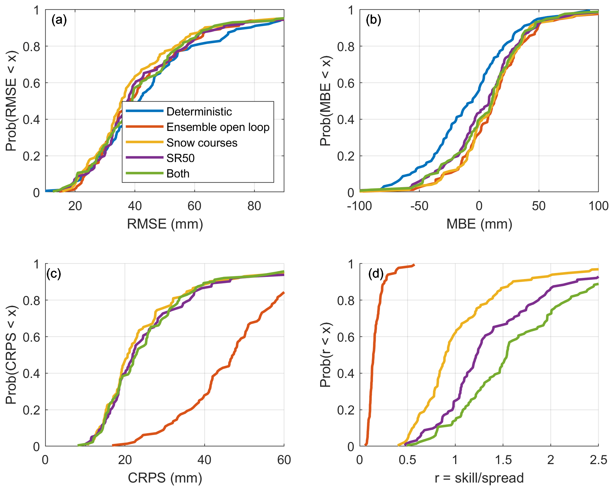
Figure 10 Cumulative distributions of the scores for the validation sites according to the nature of the assimilated data.

5 Conclusions

In this study, we propose an improvement of the spatialized particle filter introduced by Cantet et al. (2019). By reordering the particles of the filter, it was possible to slightly reduce the RMSE associated with SWE estimation at validation sites as well as to greatly improve the CRPS, which means that the uncertainty associated with SWE estimation at an ungauged site is significantly reduced. In a more general context, particle reordering is a good remedial solution to solve spatial discontinuity problems arising from resampling and localization when applying a particle filter to large spatial areas. Particle reordering may then be a new solution to the curse of dimensionality for particle filtering. To confirm this result, integration of the reordering procedures into different kinds of localized particle filters should be considered. While it has been shown that the spatialized particle filter described in this paper improved SWE estimation and provided better uncertainty estimates than previous versions or the open loop simulation, it would be beneficial to undertake a more general comparison of different localized particle filters (such as the ones described by Farchi and Bocquet, 2018 or Cluzet et al., 2021).

The reordering of particles using the Schaake shuffle technique or a sorting procedure can help maintain the spatial structure of the particles within the ensemble. The Schaake shuffle appears to be more effective at recreating the overall spatial structure of all particles. This solution makes it more reasonable to assume that it is possible to interpolate the weights of the particles in space; this is the basic assumption behind the spatialized particle filter. In cases where a sufficiently long reference record cannot be acquired, reordering by sorting the particles can provide a good alternative.

This research was also an opportunity to test the possibility of assimilating SWE estimates derived from automatic snow depth observations (SR50) and an ensemble of artificial neural networks (Odry et al., 2020). We demonstrated that the assimilation of this additional data set alone outperforms the deterministic simulation. This observation confirms the relevance of this new SWE data set. However, the assimilation of both SR50 data and snow surveys did not improve the simulation when compared with the assimilation of only the manual snow surveys. We attribute this result to the lower quality of the SWE estimates from SR50 and also to the validation process itself, which involves preserving a portion of snow survey sites for validation. Nevertheless, the exercise demonstrated the possibility of assimilating different types of data together in the spatialized particle filter, using the uncertainty associated with each type of snow observation to weight its relative influence. In this context, the current ongoing deployment in Quebec of automatic sensors capable of measuring the SWE (rather than snow depth) by using natural gamma radiation constitutes a great opportunity. Not only could this third source of information be assimilated into the particle filter, but, alternatively, it could also be used as an improved validation set, as these new gamma-ray-based sensors provide sub-daily observations, and the added value of the SR50 data in terms of temporal representativeness may be better captured. The ability of the spatialized particle filter to assimilate different types of data could also be compared to other operational assimilation frameworks such as the one described by Zhang and Yang (2016).