Ultrasonic and seismic constraints on crystallographic preferred orientations of the Priestley Glacier shear margin, Antarctica

Crystallographic preferred orientations (CPOs) are particularly important in controlling the mechanical properties of glacial shear margins. Logistical and safety considerations often make direct sampling of shear margins difficult, and geophysical measurements are commonly used to constrain the CPOs. We present here the first direct comparison of seismic and ultrasonic data with measured CPOs in a polar shear margin. The measured CPO from ice samples from a 58 m deep borehole in the left lateral shear margin of the Priestley Glacier, Antarctica, is dominated by horizontal c axes aligned sub-perpendicularly to flow. A vertical-seismic-profile experiment with hammer shots up to 50 m away from the borehole, in four different azimuthal directions, shows velocity anisotropy of both P waves and S waves. Matching P-wave data to the anisotropy corresponding to CPO models defined by horizontally aligned c axes gives two possible solutions for the c-axis azimuth, one of which matches the c-axis measurements. If both P-wave and S-wave data are used, there is one best fit for the azimuth and intensity of c-axis alignment that matches the measurements well. Azimuthal P-wave and S-wave ultrasonic data recorded in the laboratory on the ice core show clear anisotropy of P-wave and S-wave velocities in the horizontal plane that match that predicted from the CPO of the samples. With quality data, azimuthal increments of 30^∘ or less will constrain well the orientation and intensity of c-axis alignment. Our experiments provide a good framework for planning seismic surveys aimed at constraining the anisotropy of shear margins.

1 Introduction

Ice streams and glaciers are localised regions of high ice flow velocity inside otherwise mostly stationary ice masses of Antarctica and Greenland (Truffer and Echelmeyer, 2003) and play a key role in the mass balance of polar ice masses. As a result of high-velocity flow, the margins of these streaming ice bodies undergo strain as they are in contact with stationary ice or rock. Crystallographic preferred orientation (CPO) patterns observed inside glacier margins indicate a very high degree of crystal alignment in the horizontal direction (Jackson and Kamb, 1997; Monz et al., 2021; Gerbi et al., 2021; Thomas et al., 2021). These results are consistent with observations from shear deformation experiments of ice where c-axis maxima are always aligned perpendicularly to the shear plane (Bouchez and Duval, 1982; Qi et al., 2019; Journaux et al., 2019).

The presence of a CPO results in anisotropic mechanical properties and so influences the viscous behaviour of ice significantly (Azuma and Goto-Azuma, 1996; Budd et al., 2013; Faria et al., 2014; Hudleston, 2015). Shear margins of glaciers therefore can affect the character of ice flow in ice streams due to their distinct mechanical properties (Minchew et al., 2018; Hruby et al., 2020; Drews et al., 2021). The advection of the shear margins during the flow of ice from land to sea can result in bands of strongly deformed ice that transect ice shelves (LeDoux et al., 2017) and can potentially affect the stability of ice shelves. Modelling suggests that remnant CPO resultant in shear margins can be present 10 000 years after advection downstream (Lilien et al., 2021).

A better understanding of CPO patterns in glacier shear margins is therefore highly desirable to accurately determine their mechanical properties. Ice core drilling, the primary direct information source for CPO, is however rarely performed on fast-flowing ice because of difficulties in access and on-site safety. Geophysical studies, e.g. seismic (Bentley, 1971; Blankenship and Bentley, 1987; Picotti et al., 2015; Vélez et al., 2016) or radar (Matsuoka et al., 2003; Jordan et al., 2020; Ershadi et al., 2022) surveys, provide an alternative way of constraining bulk CPO. Ideally, geophysical work should be combined with drilling to recover ice samples for microstructure analysis and so enable a cross-calibration of CPO constraints.

A continuous ice core of 58 m length was drilled and recovered in December 2019 and January 2020 (Thomas et al., 2021) in a lateral shear margin of the Priestley Glacier, located in Victoria Land, Antarctica; see Fig. 1a. There is no firn layer on the glacier; however a snow cover of approximately 0.4 m was present at the time of drilling. At the site the glacier is ∼1000 m thick and 8 km wide (Frezzotti et al., 2000). Ice flow velocities are measured to increase from ∼45 m yr⁻¹ close to the glacier margin to ∼130 m yr⁻¹ towards the centre (Mouginot et al., 2019; Thomas et al., 2021), resulting in strong shear, with shear strain rates at the site calculated to be $\mathrm{6}\times {\mathrm{10}}^{-\mathrm{10}}$ s⁻¹ (Still et al., 2022; Thomas et al., 2021). Core samples were analysed for CPO using electron backscatter diffraction (EBSD) measurements (Thomas et al., 2021), and a strong horizontal clustering of c axes was observed throughout the entire length of the core. The core orientation was carefully preserved during drilling, which enabled azimuthal orientation of the CPO. The horizontal c-axis cluster orientation varies between approximately perpendicular to ice flow to 130^∘ clockwise (looking down) of the ice flow direction.

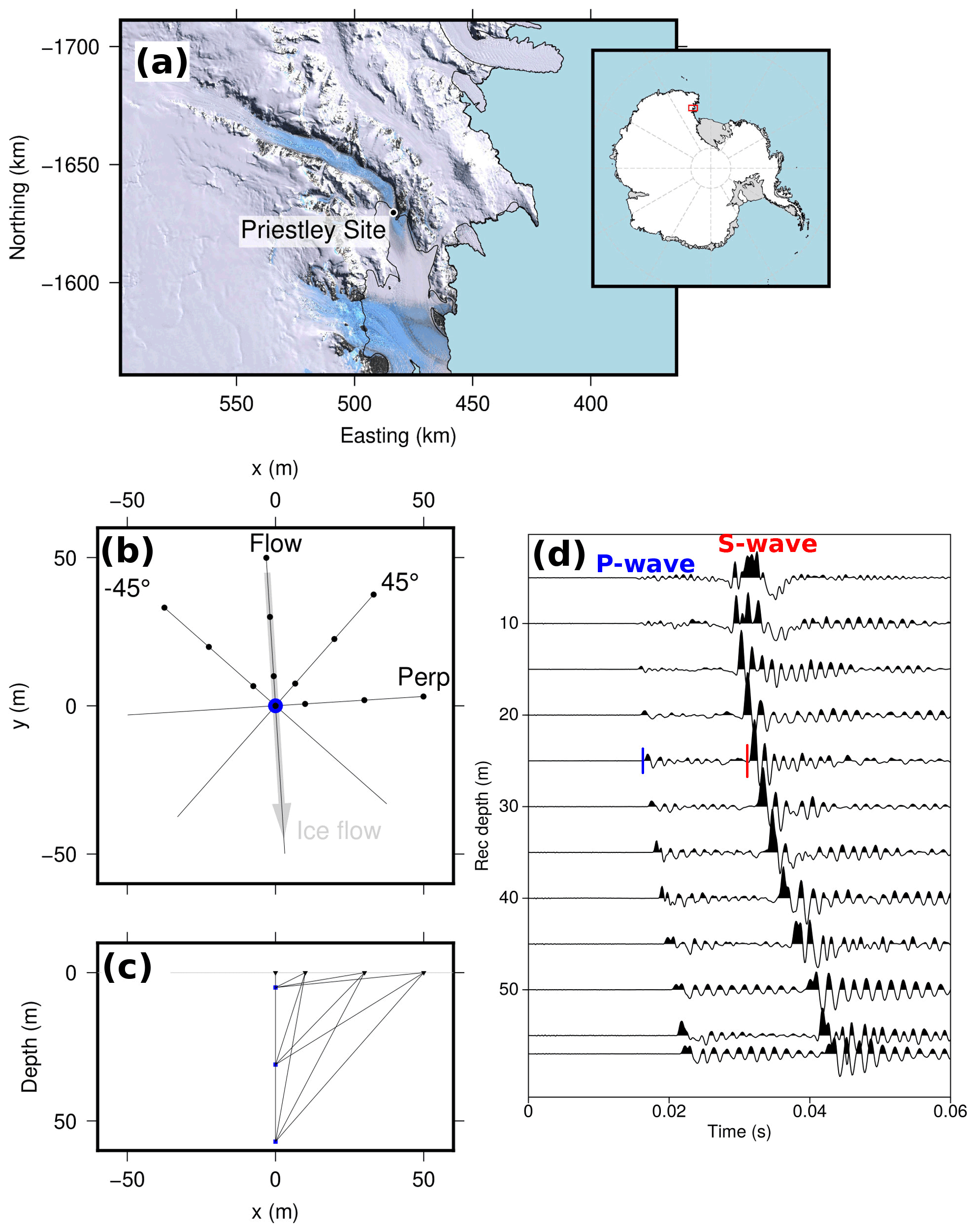
Figure 1 (a) Regional map of the Priestley Glacier site. Coordinates are given by the polar stereographic projection with latitude of true scale at $-\mathrm{71}{}^{\circ }$ S. Landsat image courtesy of USGS. (b) Map view illustration of VSP geometry. Black markers show shotpoint locations; the borehole location is shown in blue. (c) Cross-section illustration of VSP geometry showing the surface shotpoints in black and three borehole seismometer positions in blue. Lines connecting sources and receivers indicate seismic ray paths. (d) Vertical component traces of borehole seismometer for shots at 50 m offset along the 45^∘ profile. Example P- and S-wave arrival time picks are shown at 25 m depth as vertical blue and red lines.

After completion of drilling and core retrieval, the open borehole was used to conduct a vertical-seismic-profile (VSP) experiment to constrain seismic properties of the near-surface glacier ice, with a particular focus on seismic anisotropy. To complete the link between seismic anisotropy of the ice volume around the borehole and CPO measurements from the core, multi-azimuthal ultrasonic velocity measurements (Langway et al., 1988; Hellmann et al., 2021) were made on core samples in the laboratory. The anisotropy of single ice crystals displays hexagonal symmetry; i.e. wave velocity is only dependent on the angle between the propagation direction and c axis, with the fast P-wave propagation direction parallel to the c axis (Gammon et al., 1983). Seismic P- and S-wave velocities at different propagation angles relative to the c axis of a single crystal are shown in Fig. 2.

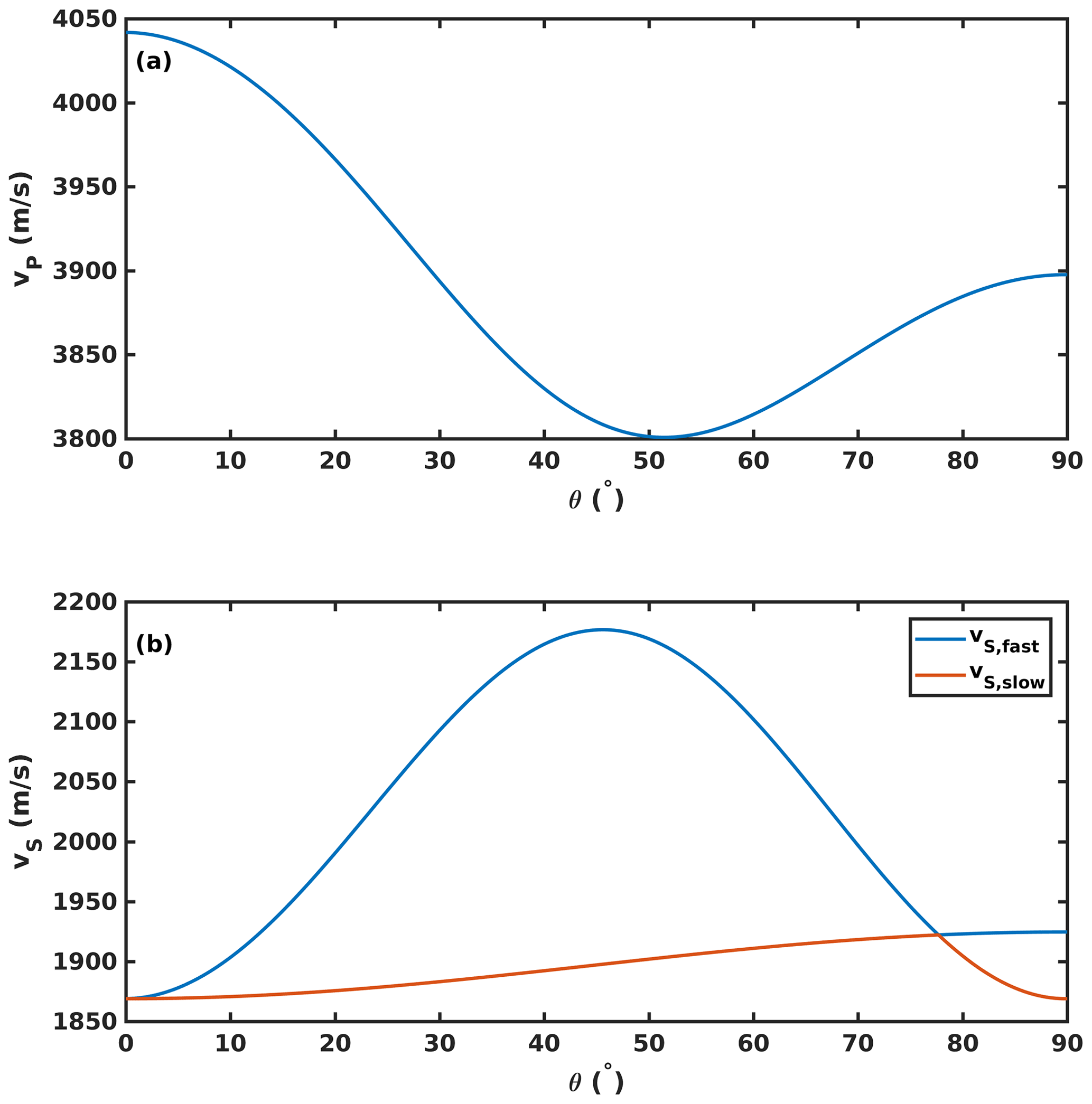
Figure 2 Seismic phase velocities for a single crystal dependent on angle θ to the c axis, calculated with values for the elastic constants from adiabatic single-crystal artificial water ice at −16 ^∘C from Gammon et al. (1983) using the MTEX toolbox (Mainprice et al., 2011). (a) P-wave velocity v_P. (b) S-wave velocities v_S.

This is the first study of the horizontal-cluster CPO type observed in shear margins with seismic methods. Analyses of seismic, ultrasonic and measured CPO datasets are combined to assess the potential of active-source seismic surveys for the constraint of shear margin anisotropy.

2 Analysis of a vertical seismic profile

2.1 Data acquisition

A VSP dataset was recorded at the Priestley drill site using a three-component borehole seismometer (built by ESS Earth Sciences, Victoria, Australia) with a pneumatic clamping system which was installed at depths z between 5 and 57 m below the glacier surface. The suspension cable, to the centre of the seismometer, remained close to the centre of the hole at the surface for all seismometer depths, indicating true verticality of the borehole. Signals from a hammer-and-plate source were recorded using a Geometrics Geode for a walkaway-VSP geometry along four profiles with different azimuths, where shots were placed at offsets x of 0 m (“zero-offset” geometry), 10, 30 and 50 m from the top of the borehole. Profile names (“Flow”, “Perp”, “45^∘”, “$-\mathrm{45}{}^{\circ }$”) indicate their orientation relative to the glacier flow direction (see Table 1). The survey geometry is illustrated in Fig. 1b. The depth increments of the borehole seismometer along the four profiles are shown in Table 1.

Table 1 Multi-azimuth VSP survey parameters.

Geode data recording for each shot in the field was initiated by a Geometrics switch trigger taped to the sledgehammer handle. Quality control of traces in the field found that this trigger type produces inconsistent zero times; i.e. repeat shots for a given source–receiver pair exhibit different arrival times. To enable the determination of absolute velocities, the recorded signal from surface geophones, collocated at the shotpoints, was used to define shot times. The Geode was set to record 100 ms before the hammer switch trigger signal to enable recording of the full first-arrival signal on the shotpoint surface geophone. Manual picking of the first-arrival time on the shotpoint surface geophone trace gives the time of hammer impact and so the true source time. Total recording length was 2 s with a sampling rate of 8000 Hz. Shot and geophone locations were cleared of all snow cover to ensure direct contact of source and receivers with the hard ice surface. Several repeat shots were recorded at all shotpoints along a given profile for one seismometer depth before the instrument was lowered to the next depth. After all shots for all seismometer depths were completed for a profile, surface geophones were moved to the next profile position.

Polarisation patterns indicate a ringing effect of the pneumatic borehole seismometer, where phase arrivals are followed by a tail of mono-frequent oscillations (see traces in Fig. 1d). The oscillations are distributed along all three seismometer components, even after separation of P- and S-wave signals through component rotation into ray coordinates (Wüstefeld et al., 2010). This noise in the phase arrival signals impedes investigating polarisation patterns, such as S-wave splitting, as a constraint on seismic anisotropy (Lutz et al., 2020).

2.2 Multi-azimuth VSP travel times

P- and S-wave first-arrival signals were recorded with a high signal-to-noise ratio, and phase arrival times can be clearly identified. Picking of seismic phase arrivals is performed manually for each shot to determine travel times: one first-arrival pick is made on the surface geophone trace at the shot location in addition to picks of P- and S-wave arrivals on the borehole seismometer traces. The P- and S-wave travel time t is then calculated as the difference between the picked arrival time on the borehole seismometer and the picked source time on the surface geophone.

Observed P-wave travel times along the seismic profiles are presented in Fig. 3a–d. The zero-offset P-wave travel times in Fig. 3a can be approximated by a constant velocity model (v_P=3850 m s⁻¹, solid line). This highlights that there is little velocity variation due to heterogeneity in the shallow glacier ice.

Differences in travel times between the profiles become apparent for shots at offsets ≥30 m and below seismometer depths of ∼25 m. The Flow and $-\mathrm{45}{}^{\circ }$ profiles show consistently earlier P-wave arrivals than the Perp and 45^∘ profiles.

Observed S-wave travel times are presented in Fig. 3f–h for shots from the four walkaway VSPs. Signal-to-noise ratios from zero-offset shots were found to be insufficient to allow picking of S-wave arrivals, likely a consequence of the radiation patterns of a plate seismic source which produces no S-wave energy in the vertical direction. The first indication of S-wave arrivals was picked consistently; travel times are therefore interpreted to be representative of the fast S-wave velocity v_S1. Systematic travel time differences between profiles are observed particularly for shots from a 50 m offset, where the $-\mathrm{45}{}^{\circ }$ profile shows the earliest arrival times over almost the entire depth range. Only for seismometer depths below 50 m are travel times from the Perp profile measured at the same time as or earlier than travel times from along the $-\mathrm{45}{}^{\circ }$ profile. The Flow and 45^∘ profiles show similar travel times that are slower than the travel times along the other profiles.

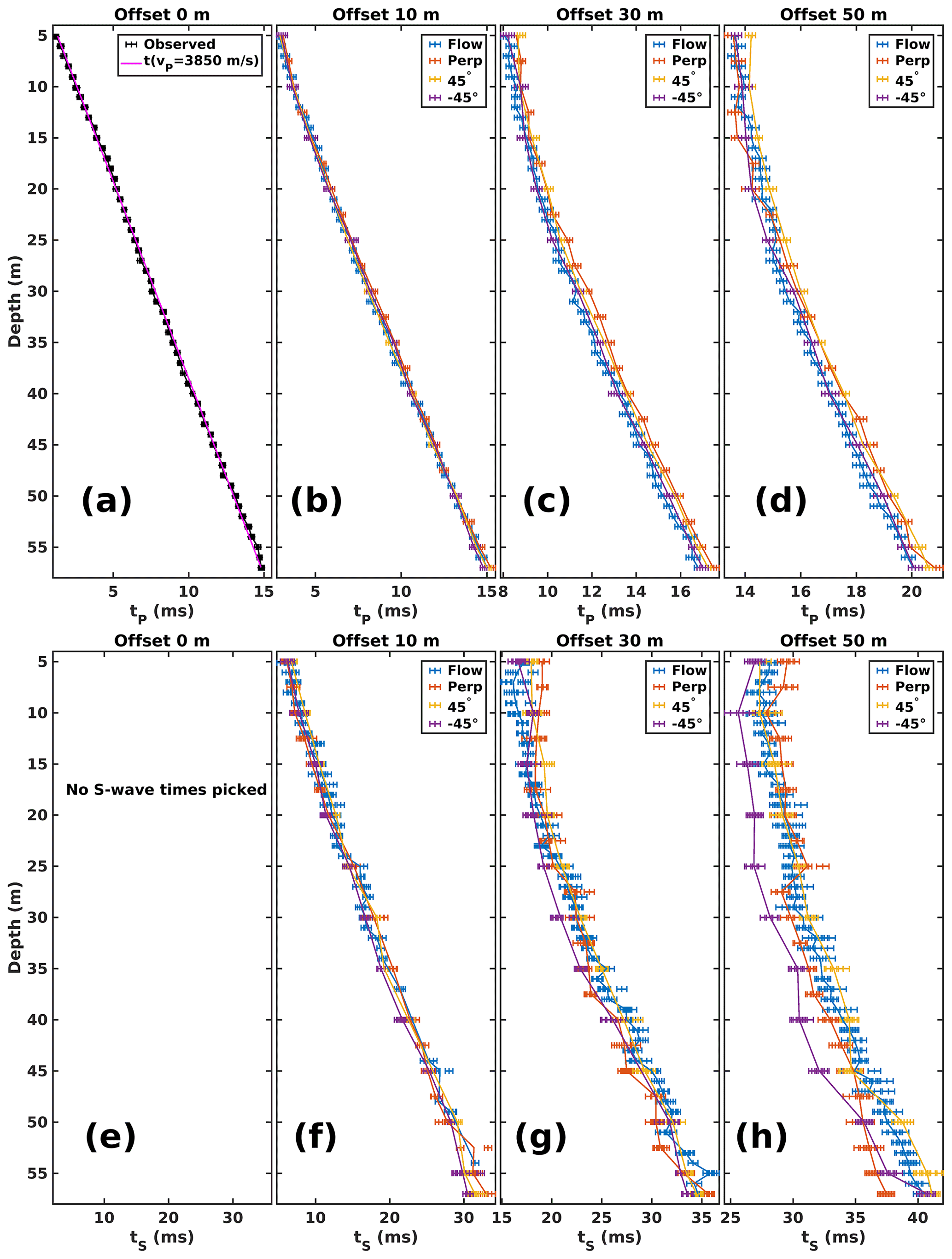
Figure 3 VSP travel times observed along the four shot profiles. (a) P-wave travel times for shots from 0 m offset. (b) P-wave travel times for shots from 10 m offset. (c) P-wave travel times for shots from 30 m offset. (d) P-wave travel times for shots from 50 m offset. (e) No S-wave travel times were picked from 0 m offset shots due to a poor signal-to-noise ratio. (f) S-wave travel times for shots from 10 m offset. (g) S-wave travel times for shots from 30 m offset. (h) S-wave travel times for shots from 50 m offset.

2.3 Velocity calculation

Seismic velocities are calculated from the presented travel times for different depths z, offsets x and azimuths in Fig. 3:

$$\begin{array}{}\text{(1)}& {\displaystyle }v={\displaystyle \frac{\sqrt{x^{\mathrm{2}}+z^{\mathrm{2}}}}{t}}.\end{array}$$

The calculation is based on the assumption of straight ray paths between the shot and receiver, which is regarded as a valid approximation for a site location on hard ice without snow cover. The seismic waves travel entirely in ice, and no large velocity gradients that could result in significant ray path bending are therefore expected (Gusmeroli et al., 2013). The zero-offset travel times in Fig. 3a exhibit no apparent indications of velocity gradients since they can be approximated by a constant vertical P-wave velocity. We therefore assume the ice volume sampled by the VSP experiment to be characterised by a homogeneous, constant-CPO layer. The incidence angle θ from the vertical direction is defined as

$$\begin{array}{}\text{(2)}& {\displaystyle }\mathit{\theta }=\arctan \left({\displaystyle \frac{x}{z}}\right).\end{array}$$

Velocity uncertainties Δv are calculated from uncertainty estimates for P-wave travel time Δt_P=0.125 ms, S-wave travel time Δt_S=1 ms, offset Δx=0.2 m and depth Δz=0.1 m.

$$\begin{array}{}\text{(3)}& \mathrm{\Delta }v={\displaystyle \frac{x\mathrm{\Delta }x+z\mathrm{\Delta }z}{t\cdot \sqrt{x^{\mathrm{2}}+z^{\mathrm{2}}}}}+{\displaystyle \frac{\mathrm{\Delta }t\cdot \sqrt{x^{\mathrm{2}}+z^{\mathrm{2}}}}{t^{\mathrm{2}}}}\end{array}$$

Observations with relative uncertainty $\mathrm{\Delta }v/v>\mathrm{0.05}$ are discarded from further analysis.

3 Analysis of ultrasonic experiments

Ultrasonic experiments were performed inside a freezer at the temperature $-\mathrm{23}\pm \mathrm{2}$ ^∘C on a subset of samples from the continuous ice core. Samples were lathed to the shape of a highly regular cylinder. Travel time measurements were made perpendicularly to the core axis in multiple azimuths to measure ultrasonic velocities in the horizontal direction of the glacier ice. Olympus ultrasonic P- or S-wave transducers were spring-loaded against the cylinder surface, on opposing sides of the cylinder (Fig. 4a and b). S-wave transducers were used for excitation and recording of S waves with polarisations in the vertical (parallel to the long core axis) and horizontal (perpendicular to the long core axis) direction. Coupling of transducers to the ice core samples was ensured through the use of synthetic high-performance low-temperature grease.

Travel time measurements across the ice core were made in azimuthal increments of 10^∘ covering the full core diameter, resulting in N=36 measurements per transducer arrangement and core. A fiducial line that was made in the field to provide geographic reference of the core orientation served as the 0^∘ reference on individual samples. The fiducial line was made perpendicularly to the glacier flow direction on the surface (Thomas et al., 2021). New fiducial lines were started wherever a core break could not be fitted together, and the relative orientations of the lines were reconstructed using the core CPO (Thomas et al., 2021). Measurements are on core sections 003 from a depth of ∼2.5 m (diameter $d=\mathrm{100.6}\pm \mathrm{0.3}$ mm), 007 from a depth of ∼6.0 m (diameter $d=\mathrm{99.9}\pm \mathrm{0.3}$ mm) and 010 from a depth of ∼8.5 m (diameter $d=\mathrm{100.3}\pm \mathrm{0.3}$ mm). The in situ temperature at the sample depths was observed to be between $\approx -\mathrm{7}$ and $\approx -\mathrm{15}$ ^∘C (Thomas et al., 2021). Ultrasonic measurements made at these warmer temperatures did not result in any measurable effect on seismic anisotropy. Since warmer temperatures caused problems with transducer coupling to the ice cores, the initially described freezer temperature setting at $-\mathrm{23}\pm \mathrm{2}$ ^∘C was used for the ultrasonic experiments.

The ultrasonic source signal pulse was created by a JSR Ultrasonics DPR300 pulser unit and shows a dominant frequency f≈1 MHz, resulting in a dominant wavelength of λ≈3.8 mm in the ice. Recording of the source and receiver signal was performed on separate oscilloscope channels by a PicoScope digital oscilloscope with a sampling interval t_S=0.8 ns. Signals were recorded directly by the oscilloscope without the use of amplifiers. The source signal was used to trigger signal recording by exceedance of an amplitude threshold. A signal length of 100 µs after triggering is recorded.

3.1 Processing

At each azimuth 64 individual waveforms were recorded. The mean amplitude and linear trend are removed from these individual traces before they are stacked to increase the signal-to-noise ratio. The stacked traces are tapered and filtered with a bandpass filter with corner frequencies f₁ = 50 KHz and f₂=5 MHz and normalised for plotting.

Waveforms recorded on sample 007 are shown in Fig. 4c–e. The core orientation angle in these plots is relative to the fiducial marker on the core sample. Recorded waveforms using the P-wave transducers are shown in Fig. 4c. A rotational symmetry with periodicity of 180^∘ is present, which confirms a consistent and reliable excitation and recording of P-wave signals for all azimuths around the core.

Waveforms recorded using S-wave transducers set for vertical vibration are shown in Fig. 4d, indicating a clear periodicity of 180^∘ and are predominantly indicative of the slow S-wave velocity v_S2.

Waveforms from S-wave transducers set for horizontal vibration are shown in Fig. 4e. Here, four local maxima in velocity are observed for the full range of azimuths. This arrangement of transducers enables the measurement of fast S-wave velocity v_S1 at most azimuths.

Figure 4 (a) Side view of ultrasonic rig with slots for different transducer orientations highlighted. (b) Map view of ultrasonic rig. Transducers are set for vertical vibration. (c) Multi-azimuth signal traces using P-wave transducers on sample 007. (d) Multi-azimuth signal traces using S-wave transducers set for vertical vibration on sample 007. (e) Multi-azimuth signal traces using S-wave transducers set for horizontal vibration on sample 007.

3.2 P-wave and S-wave ultrasonic velocity results

Arrival times t of the direct P- and S-wave phases are picked by hand on the stacked traces and used to calculate ultrasonic velocities $v=d/t$. Successful measurements of v_P, v_S1 and v_S2 are made at all azimuths and samples, which constitute an unprecedented characterisation of ultrasonic velocity anisotropy in high detail. Velocity uncertainties are calculated from diameter uncertainty Δd=0.3 mm and picking uncertainty Δt=0.1 µs.

Ultrasonic P- and S-wave velocities of the three core sections studied are shown in Fig. 5a–c. The velocities are presented in the kinematic reference frame, where the angles relative to the fiducial lines on individual samples are transformed to give the orientation relative to glacier flow at the site (Thomas et al., 2021). The azimuth given in the plots presents the angle from the flow-parallel VSP in Fig. 1b in a clockwise direction.

The largest P- and S-wave velocities are observed in sample 007; sample 003 shows the lowest velocities, and intermediate velocities are measured in sample 010. A variation in seismic velocities with the azimuth is present in all samples. Shapes of the velocity curves are very similar for the three individual samples; however the observed velocities of 003 are shifted by an angle of $\approx \mathrm{20}{}^{\circ }$ relative to the curves of 007 and 010.

Ultrasonic v_P measurements were also made along the core axis, sampling the vertical direction at the temperature $-\mathrm{23}\pm \mathrm{2}$ ^∘C. Sample velocities of $v_{\mathrm{P},\mathrm{vert},\mathrm{003}}$ = 3838 ± 20 m s⁻¹, $v_{\mathrm{P},\mathrm{vert},\mathrm{007}}$ = 3822 ± 15 m s⁻¹ and $v_{\mathrm{P},\mathrm{vert},\mathrm{010}}=\mathrm{3842}\pm \mathrm{18}$ m s⁻¹ again highlight near-constant velocity with depth implicit in the zero-offset VSP P-wave travel times (Fig. 3a). The range of vertical v_P is shown in Fig. 5a. The observation that vertical v_P is faster than horizontal v_P for most azimuths is inconsistent with the expected velocities for a horizontal-cluster CPO, and no definite explanation for this observation is available at this point. Potential additional influences on velocities could be given by populations of “oddly” oriented grains (Thomas et al., 2021) that show orientations in the horizontal plane but outside of the c-axis cluster. They could therefore reduce the maximum v_P along the cluster axis but not affect v_P in the vertical direction. Anisotropy related to preferred bubble shape or aligned cracks, both observed in the uppermost ≈10 m of the ice core (Thomas et al., 2021), could also play a role.

An attempted measurement of v_S in the vertical direction failed because no clear ultrasonic S-wave signals that allowed travel time picking could be recorded in this geometry.

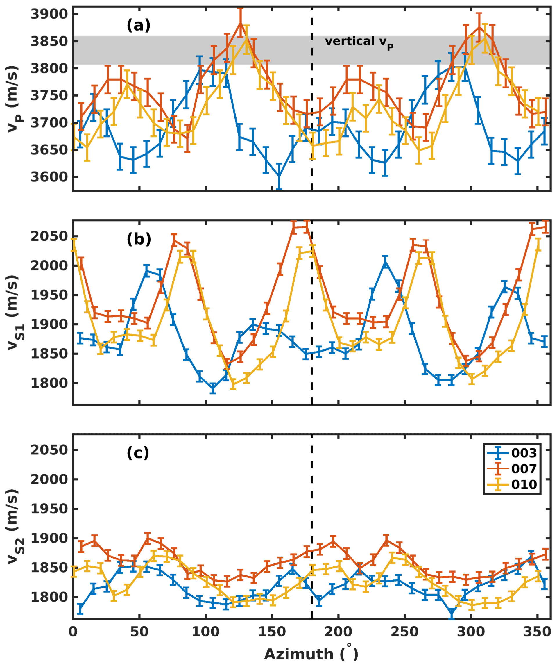
Figure 5 Ultrasonic multi-azimuth velocities for different core sections relative to the macroscopic glacier flow direction (0^∘). (a) P-wave velocity v_P. The grey-shaded box shows the range of measured vertical ultrasonic v_P. (b) Fast S-wave velocity v_S1. (c) Slow S-wave velocity v_S2.

4 CPO modelling

The observed high degree of seismic anisotropy in VSP seismic and multi-azimuth ultrasonic data is consistent with the observation of strong CPO in the retrieved core samples from the site. EBSD measurements on core samples constrain the CPO to be characterised by a strong clustering of c axes in the horizontal plane (Thomas et al., 2021). The availability of constraints from sample microscopic analysis and geophysical data at the Priestley Glacier site is therefore suitable for a calibration of seismic properties to the known CPO. The observed P- and S-wave velocity anisotropies from VSP and multi-azimuth ultrasonic observations are compared to models of polycrystal elasticity connected to CPOs comprising horizontally clustered c axes. In general, when interpreting geophysical data, no CPO constraints are available and a range of different CPO geometries have to be tested to match observations (Diez and Eisen, 2015; Maurel et al., 2015; Lutz et al., 2020). We skip this step and focus entirely on the influence of survey geometry and suitability of P- and S-wave velocity information for constraining ice CPO.

4.1 Horizontal-cluster CPO

CPO models are created using the MTEX toolbox for MATLAB (Mainprice et al., 2011), consisting of 1000 clustered c axes with the cluster symmetry axis in the horizontal direction. A geometrical description of this horizontal-cluster CPO forward model can be given by a diffused cluster with the symmetry axis in the horizontal plane. The model parameters of this cluster geometry are defined by the azimuth φ of the cluster symmetry axis and the cluster width angle α. An illustration of this CPO type is presented in Fig. 6 in an upper-hemisphere stereographic projection.

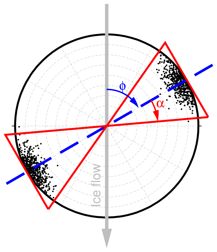
Figure 6 Upper-hemisphere stereographic projection c-axis orientations of an example horizontal-cluster CPO model with illustration of model parameters: cluster orientation φ and opening angle α.

Seismic properties of individual crystals are characterised by the elasticity tensor C in Eq. (4) of synthetic ice at −16 ^∘C by Gammon et al. (1983) and density ρ=919.1 kg m⁻³. For any given set of CPO model parameters φ and α, synthetic seismic velocities associated with the CPO are calculated after forming the Voigt–Reuss–Hill average elastic properties (Hill, 1952; Mainprice, 2007).

$$\begin{array}{}\text{(4)}& \begin{array}{rl}& C=\\ & \left[\begin{array}{cccccc}\mathrm{13.913}& \mathrm{7.026}& \mathrm{5.801}& \mathrm{0}& \mathrm{0}& \mathrm{0}\\ \mathrm{7.026}& \mathrm{13.913}& \mathrm{5.801}& \mathrm{0}& \mathrm{0}& \mathrm{0}\\ \mathrm{5.801}& \mathrm{5.801}& \mathrm{15.059}& \mathrm{0}& \mathrm{0}& \mathrm{0}\\ \mathrm{0}& \mathrm{0}& \mathrm{0}& \mathrm{3.011}& \mathrm{0}& \mathrm{0}\\ \mathrm{0}& \mathrm{0}& \mathrm{0}& \mathrm{0}& \mathrm{3.011}& \mathrm{0}\\ \mathrm{0}& \mathrm{0}& \mathrm{0}& \mathrm{0}& \mathrm{0}& \mathrm{3.4435}\end{array}\right]\text{ GPa}\end{array}\end{array}$$

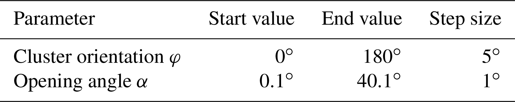
Model parameters φ and α are systematically varied in regular step sizes, and all combinations within the individual parameter ranges presented in Table 2 are explored. Synthetic seismic properties are compared to observations for each model realisation.

Table 2 Horizontal-cluster CPO model parameters.

4.2 Model misfit calculation

The ability of a CPO model to explain measured seismic anisotropy is assessed by introduction of a misfit between synthetic forward-modelled seismic properties and observations. We found that CPO-predicted seismic velocities are consistently faster than observed velocities, an effect which can be attributed to the absence of grain boundary effects (Sayers, 2018) or air bubbles (Hellmann et al., 2021) in synthetic CPOs. The elasticity tensor by Gammon et al. (1983) was derived using oscillations in gigahertz (GHz) frequencies; therefore dispersion is another potential factor to introduce differences between modelled and observed seismic or ultrasonic velocities with hertz (Hz) to kilohertz (kHz) frequencies. A normalisation is introduced to address these described effects on absolute velocities, and we focus entirely on modelled and observed anisotropic velocity variations rather than absolute velocities, studying the variation in velocities relative to the mean velocity. This definition of seismic anisotropy δv is given in Eq. (5), where $\overline{v}$ is the mean wave velocity of all observations.

$$\begin{array}{}\text{(5)}& \mathit{\delta }v=\left({\displaystyle \frac{v}{\overline{v}}}-\mathrm{1}\right)\cdot \mathrm{100}\end{array}$$

We consider the elasticity data from Gammon et al. (1983) to provide high accuracy of relative velocity variation. Therefore we have chosen to rely upon these data, and no other published elasticities of ice are investigated to match the observed anisotropy as has been done in previous studies which have compared absolute measured and synthetic velocities (Diez et al., 2015; Picotti et al., 2015). A misfit χ_raw is calculated by Eq. (6) between measured (δv) and synthetic (δv_M) velocity variations. N is the number of velocity observations.

$$\begin{array}{}\text{(6)}& {\mathit{\chi }}_{\mathrm{raw}}\left(v\right)=\sqrt{{\displaystyle \frac{\mathrm{1}}{N}}\sum _{i=\mathrm{1}}^N{\left(\mathit{\delta }{v}_i-\mathit{\delta }{v}_{M,i}\right)}^{\mathrm{2}}}\end{array}$$

Misfits χ_raw(v) are calculated individually for the v_P, v_S1 and v_S2 observations and all synthetic CPO models. The χ(v_P), χ(v_S1) and χ(v_S2) misfits are then calculated through division by the largest misfit of all models.

$$\begin{array}{}\text{(7)}& \mathit{\chi }\left(v\right)={\mathit{\chi }}_{\mathrm{raw}}\left(v\right)/\text{max}\left({\mathit{\chi }}_{\mathrm{raw}}\right(v\left)\right)\end{array}$$

In addition, misfit averages are defined as

$$\begin{array}{ll}{\displaystyle }& {\displaystyle }\mathit{\chi }\left(v_{\mathrm{P}}\right)+\mathit{\chi }\left(v_{\mathrm{S}\mathrm{1}}\right)=\\ \text{(8)}& {\displaystyle }& {\displaystyle }{\displaystyle \frac{\mathrm{1}}{\mathrm{2}}}\left({\displaystyle \frac{{\mathit{\chi }}_{\mathrm{raw}}\left(v_{\mathrm{P}}\right)}{\text{max}\left({\mathit{\chi }}_{\mathrm{raw}}\right(v_{\mathrm{P}}\left)\right)}}+{\displaystyle \frac{{\mathit{\chi }}_{\mathrm{raw}}\left(v_{\mathrm{S}\mathrm{1}}\right)}{\text{max}\left({\mathit{\chi }}_{\mathrm{raw}}\right(v_{\mathrm{S}\mathrm{1}}\left)\right)}}\right),{\displaystyle }& {\displaystyle }\mathit{\chi }\left(v_{\mathrm{P}}\right)+\mathit{\chi }\left(v_{\mathrm{S}\mathrm{1}}\right)+\mathit{\chi }\left(v_{\mathrm{S}\mathrm{2}}\right)=\\ \text{(9)}& {\displaystyle }& {\displaystyle }{\displaystyle \frac{\mathrm{1}}{\mathrm{3}}}\left({\displaystyle \frac{{\mathit{\chi }}_{\mathrm{raw}}\left(v_{\mathrm{P}}\right)}{\text{max}\left({\mathit{\chi }}_{\mathrm{raw}}\right(v_{\mathrm{P}}\left)\right)}}+{\displaystyle \frac{{\mathit{\chi }}_{\mathrm{raw}}\left(v_{\mathrm{S}\mathrm{1}}\right)}{\text{max}\left({\mathit{\chi }}_{\mathrm{raw}}\right(v_{\mathrm{S}\mathrm{1}}\left)\right)}}+{\displaystyle \frac{{\mathit{\chi }}_{\mathrm{raw}}\left(v_{\mathrm{S}\mathrm{2}}\right)}{\text{max}\left({\mathit{\chi }}_{\mathrm{raw}}\right(v_{\mathrm{S}\mathrm{2}}\left)\right)}}\right).\end{array}$$

4.3 CPO model fit using VSP velocities

The model misfit of the VSP data is calculated using N_P=1354 and N_S1=1036 velocity observations. Figure 7a shows the model misfits based on P-wave velocities χ(v_P). The best-fitting model is indicated by the red dot. This model CPO is shown in Fig. 7d. Figure 7b and e show S-wave misfits χ(v_S1) and the corresponding best-fitting CPO model. The misfit average χ(v_P)+χ(v_S1) is presented in Fig. 7c, with its best-fitting CPO model presented in Fig. 7f. Parameters of the best-fitting CPO models based on VSP observations are provided in Table 3. Parameter uncertainties are taken from the range of models that produce the minimum 1 % of misfits.

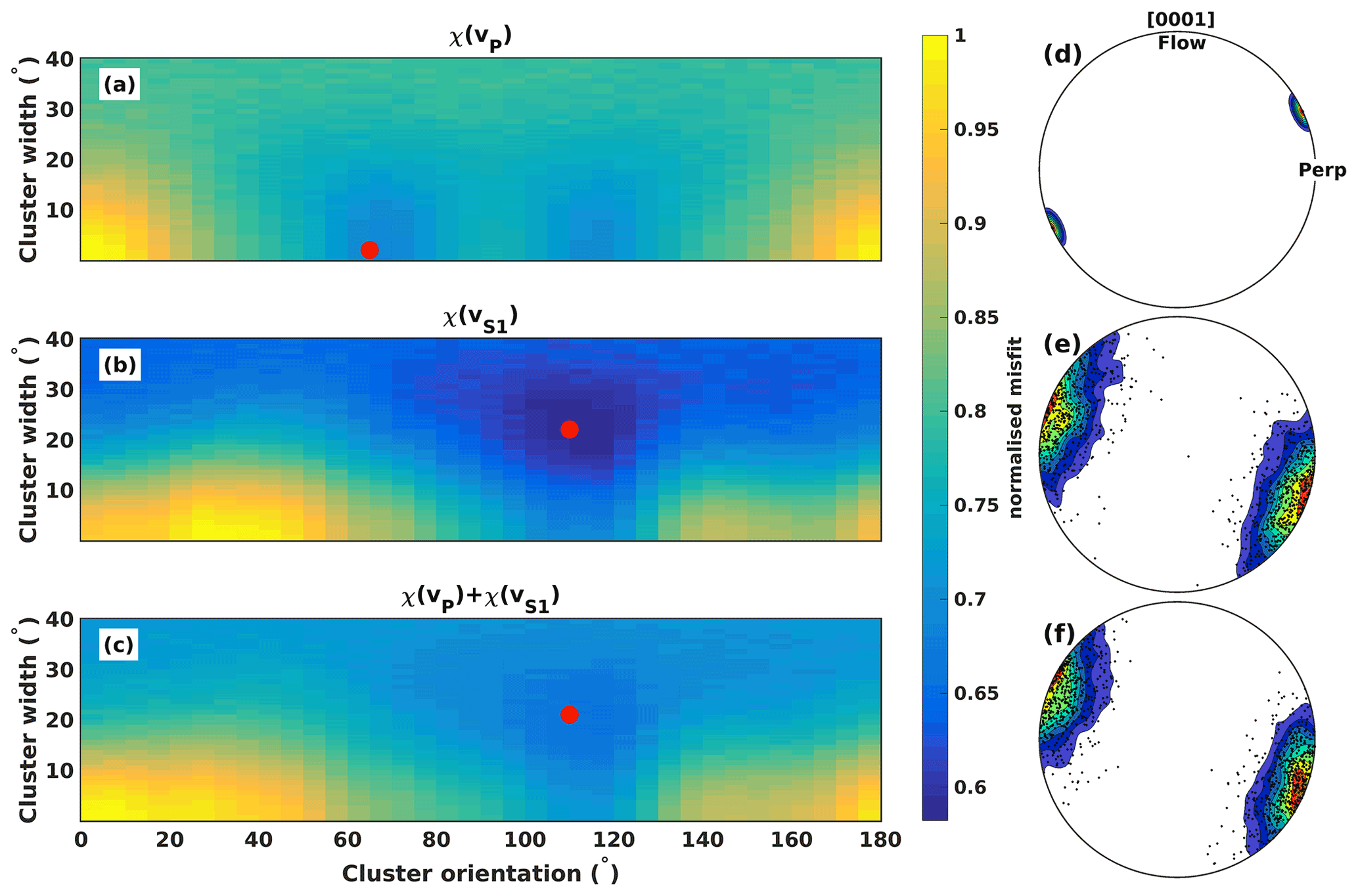
Figure 7 (a) Misfit surface considering only P-wave velocities. (b) Misfit surface considering only S-wave velocities. (c) Misfit surface considering P- and S-wave velocities. (d) Best-fitting CPO model result considering only P-wave velocities. Contour lines indicate c-axis density in an upper-hemisphere stereographic projection. Labels indicate the orientation of the Flow and Perp profile shots in the VSP survey (compare Fig. 1b). (e) Best-fitting CPO model result considering only S-wave velocities. (f) Best-fitting CPO model result considering P- and S-wave velocities.

Table 3 Best-fitting CPO model parameters and uncertainties informed by VSP data.

Figure 8 shows the observed P-wave anisotropy δv_P (symbols) along the four survey profiles together with predicted anisotropy from the CPO models presented in Table 3 (dashed lines). The observed variation in velocities with incidence angle is consistent across all seismometer depths, strengthening the assumption that no change in CPO with depth is present within the investigated ice volume. Modelled anisotropies generally match observations within uncertainties along the Flow, Perp and $-\mathrm{45}{}^{\circ }$ profiles. It is notable that the three different models exhibit very similar seismic properties along these profiles, although the CPO model informed by χ(v_P) in Fig. 7d shows a fundamentally different geometry than the CPO models shown in Fig. 7e and f. The $-\mathrm{45}{}^{\circ }$ profile shows a larger difference between the models with a steady decrease in δv_P predicted by the models informed by χ(v_S1) and χ(v_P)+χ(v_S1), while the χ(v_P) CPO model suggests a decrease in δv_P to incidence angles of $\sim \mathrm{40}{}^{\circ }$, followed by increasing δv_P towards larger incidence angles. The difference between data and models is largest along this profile; however the observed δv_P values support the steady decrease in P-wave velocity between the vertical (0^∘) and horizontal incidence (90^∘) that is suggested by the χ(v_S1) and χ(v_P)+χ(v_S1) CPO models.

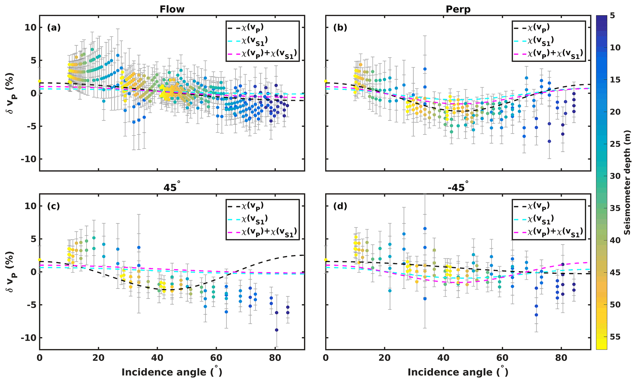
Figure 8 Multi-azimuth P-wave observed velocity anisotropy (symbols) and model results (dashed lines) along the different profiles. Symbol colour shows sensor depths. (a) Flow profile; (b) Perp profile; (c) 45^∘ profile; (d) $-\mathrm{45}{}^{\circ }$ profile.

Fast S-wave anisotropy δv_S1 observations are shown in Fig. 9 alongside the modelled anisotropy. Measured velocities exhibit a variation with incidence angle which is consistent across all seismometer depths. Again, observations and models are all in general agreement on the Flow and Perp profile, albeit with an observed decrease in δv_S1 on the Perp profile for incidence angles $\ge \mathrm{60}{}^{\circ }$ which is not satisfyingly matched by any model. The most significant differences are seen along the 45^∘ and $-\mathrm{45}{}^{\circ }$ profile: here only the models informed by χ(v_S1) and χ(v_P)+χ(v_S1) match observations, and the model informed by χ(v_P) is strongly mismatched.

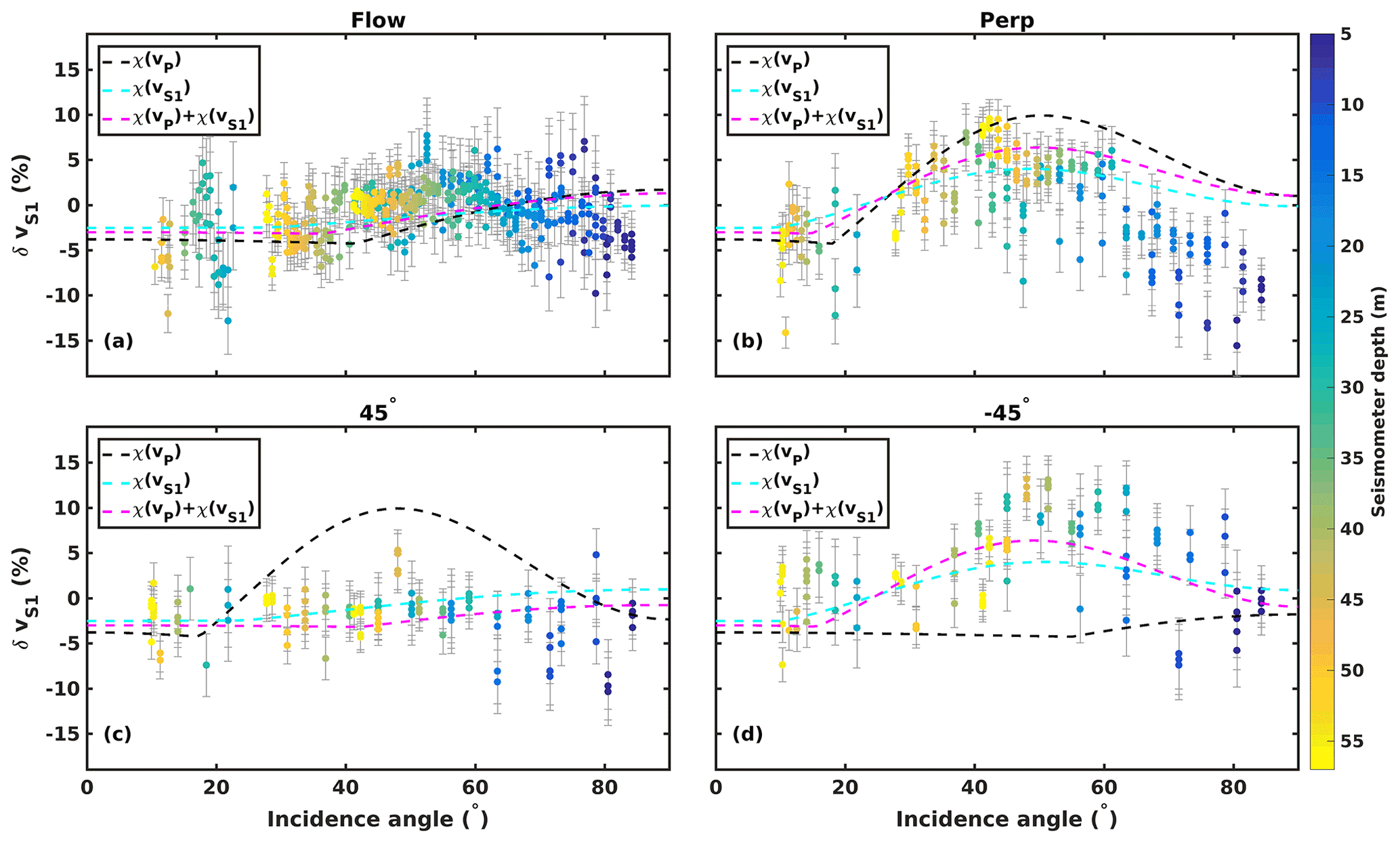
Figure 9 Multi-azimuth S-wave observed velocity anisotropy (symbols) and model results (dashed lines) along the different profiles. Symbol colour shows sensor depths. (a) Flow profile; (b) Perp profile; (c) 45^∘ profile; (d) $-\mathrm{45}{}^{\circ }$ profile.

4.4 CPO model fit using ultrasonic velocities

Misfits χ of the horizontal-cluster CPO are calculated from the multi-azimuth observations of v_P, v_S1 and v_S2 on the core samples 003, 007 and 010.

Figure 10 shows misfits χ of the different velocities for sample 003, where the red mark indicates the best-fitting model. The individual misfits in Fig. 10a–c and the sum of all misfits in Fig. 10d show best-fitting models with a consistent cluster orientation and a small scatter in reconstructed cluster opening angles. The shape of the areas of lowest misfit shows that cluster orientation can be constrained with higher confidence than cluster width. An overview of CPO model parameters informed by the ultrasonic measurements is provided in Table 4. The misfit informed by v_S1 in Fig. 10b shows a local minimum at an orientation that is $\sim \mathrm{90}{}^{\circ }$ offset from the best-fitting model. This reflects the shape of the measured v_S1 variation with the azimuth, which shows approximately 90^∘ periodicity, whereas v_P and v_S2 show 180^∘ periodicity (see Fig. 5). The sum of all misfits (Fig. 10d) is regarded as providing the most reliable constraint on model fit. Here, the local minimum present in χ(v_S1) is attenuated, which resolves the ambiguity in the CPO model constraint.

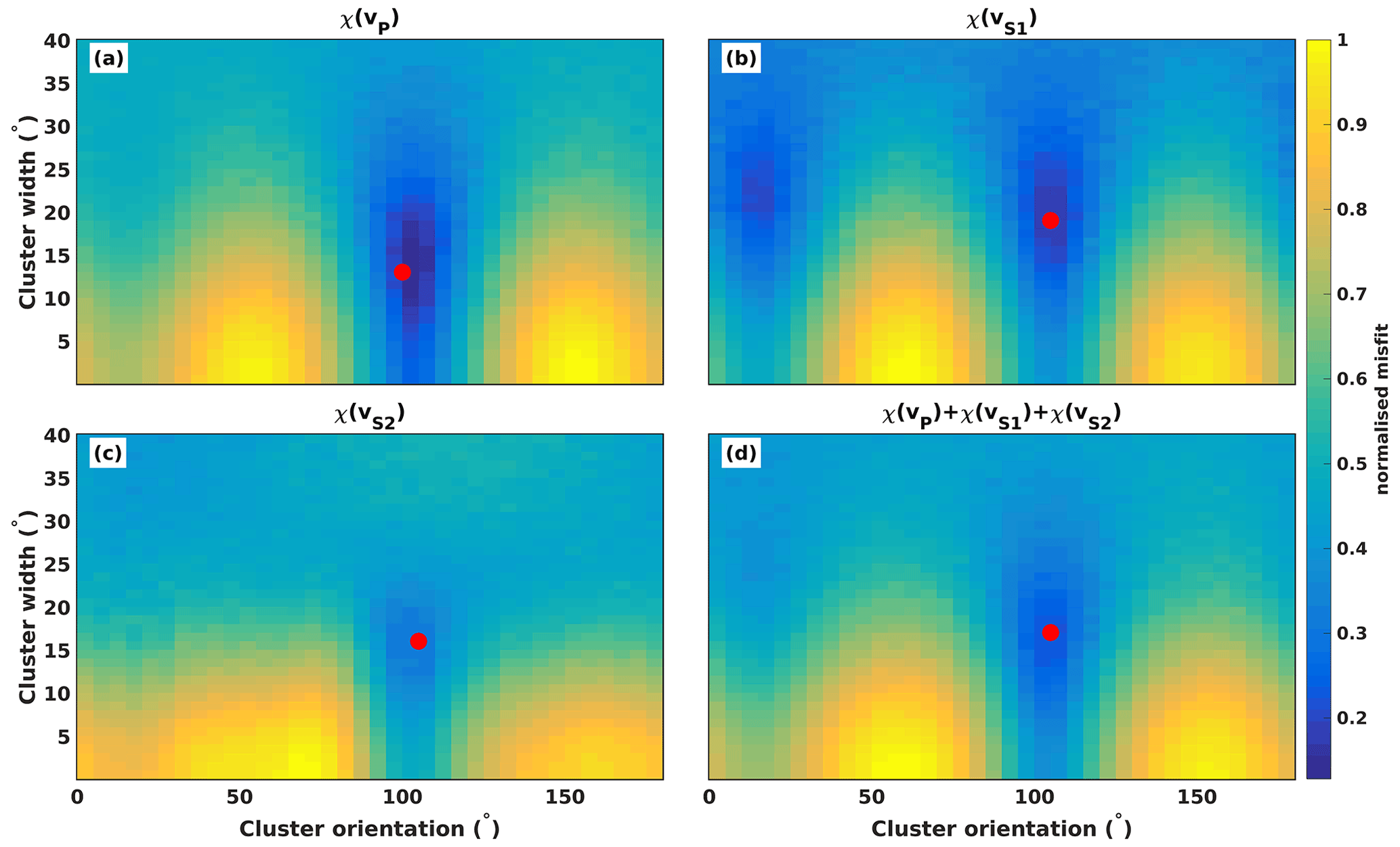
Figure 10 Misfit surfaces of seismic velocities showing fit to model parameters of the horizontal-cluster CPO for sample 003: (a) χ(v_P), (b) χ(v_S1), (c) χ(v_S2) and (d) $\mathit{\chi }\left(v_{\mathrm{P}}\right)+\mathit{\chi }\left(v_{\mathrm{S}\mathrm{1}}\right)+\mathit{\chi }\left(v_{\mathrm{S}\mathrm{2}}\right)$.

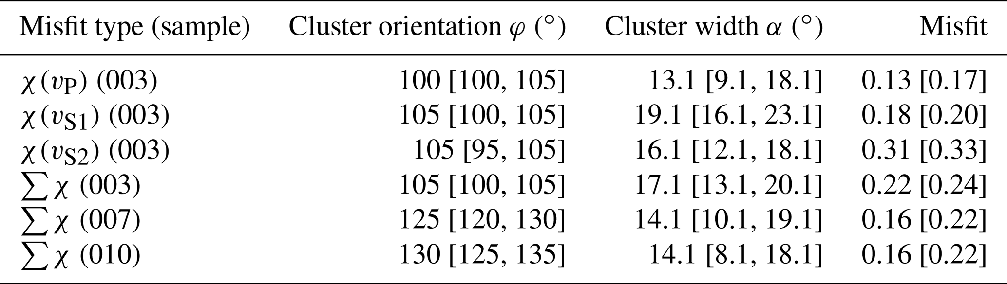
Table 4 Best-fitting CPO model parameters and uncertainties informed by ultrasonic data. The notation $\sum \mathit{\chi }=\mathit{\chi }\left(v_{\mathrm{P}}\right)+\mathit{\chi }\left(v_{\mathrm{S}\mathrm{1}}\right)+\mathit{\chi }\left(v_{\mathrm{S}\mathrm{2}}\right)$ is introduced.

The best-fitting models of the three core samples are identified by the minimum in the misfit sum $\mathit{\chi }\left(v_{\mathrm{P}}\right)+\mathit{\chi }\left(v_{\mathrm{S}\mathrm{1}}\right)+\mathit{\chi }\left(v_{\mathrm{S}\mathrm{2}}\right)$. The c-axis distribution of these CPO models is shown in upper-hemisphere plots in Fig. 11 alongside the measured CPO of the samples.

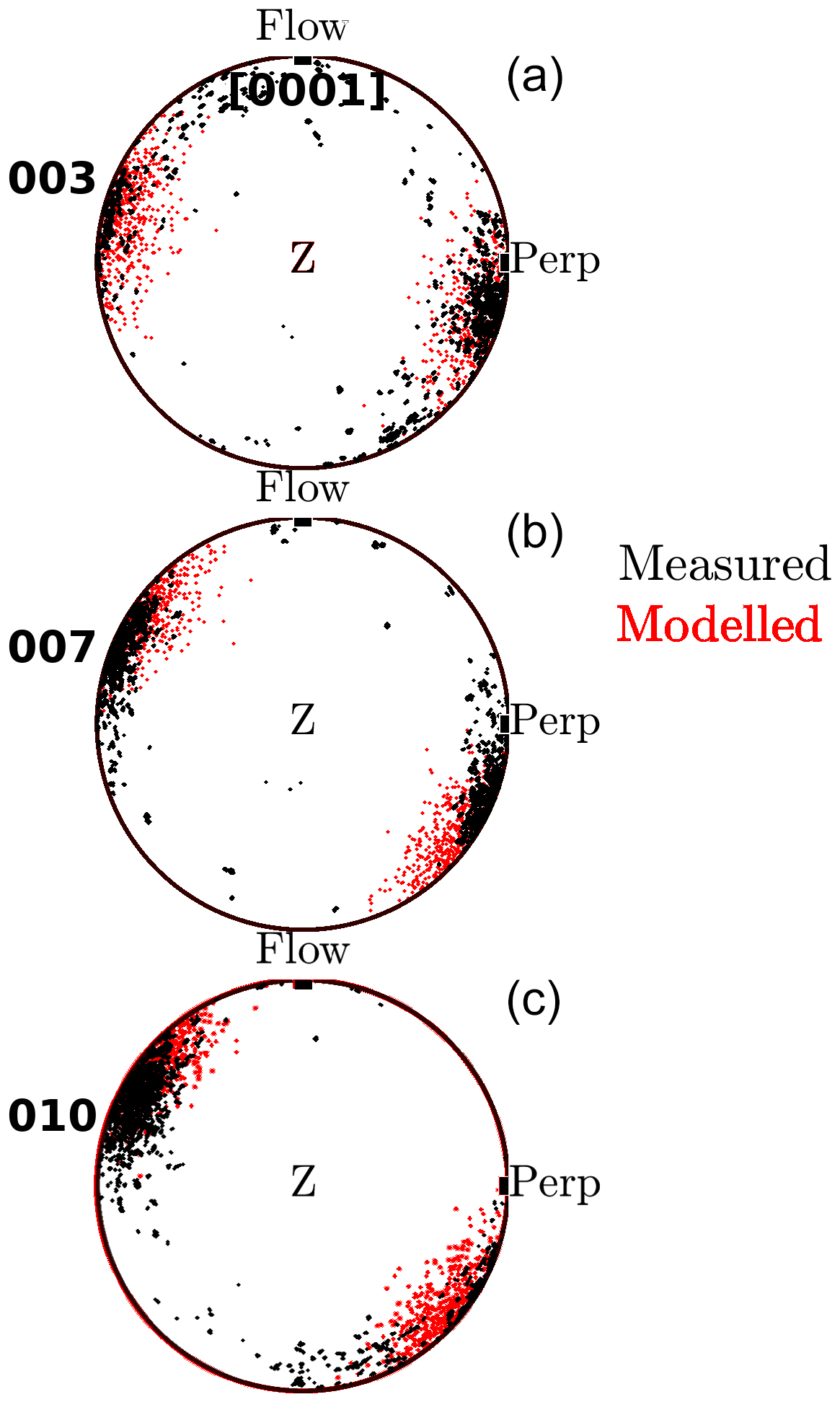
Figure 11 Measured (black) and modelled (red) CPO geometries. c-axis orientations in an upper-hemisphere stereographic projection are shown. The VSP orientations of the Flow and Perp profiles are labelled. (a) Sample 003; (b) sample 007; (c) sample 010.

5 Discussion

5.1 Horizontal-cluster reconstruction

Both the VSP data and the ultrasonic data are best matched by CPOs with cluster azimuths between 105 and 130^∘ from the macroscopic ice flow direction at the site. This is consistent with CPO measurements made on core samples using EBSD analysis (Thomas et al., 2021). The agreement in model results between ultrasonic and seismic data bridges the two different scales at which these measurements are made. Ultrasonic and EBSD measurements that are made in ice core samples are shown to be representative of anisotropy within the macroscopic volume that is sampled by the VSP survey.

The inter-sample variation in CPO cluster orientations inside the shallow ice at the site (Thomas et al., 2021) is also clearly visible in the ultrasonic velocity variation: Fig. 5 shows that the ultrasonic velocities in the three samples follow similar patterns, which are slightly offset between the individual samples. Different fast seismic directions in the studied samples are apparent in Fig. 5, especially between sample 003 and samples 007 and 010. Consequently the CPO model of 003 shows a different cluster azimuth than the models of samples 007 and 010 in Fig. 11.

Figure 11 also shows that the c-axis maxima modelled from seismic anisotropies for samples 007 and 010 are rotated around the vertical axis relative to CPO measurements. The measured and modelled CPOs of sample 003 show excellent agreement; however for samples 007 and 010 the modelled CPO clusters are slightly rotated in a clockwise direction relative to the measured CPO geometry. Using the EBSD-measured c-axis orientations, a forward model of velocity anisotropy is calculated with MTEX. A comparison of observed and forward-modelled velocity variations is given for sample 003 in Fig. 12, which highlights that the constrained CPO model explains measured and CPO-predicted seismic anisotropy to a high degree.

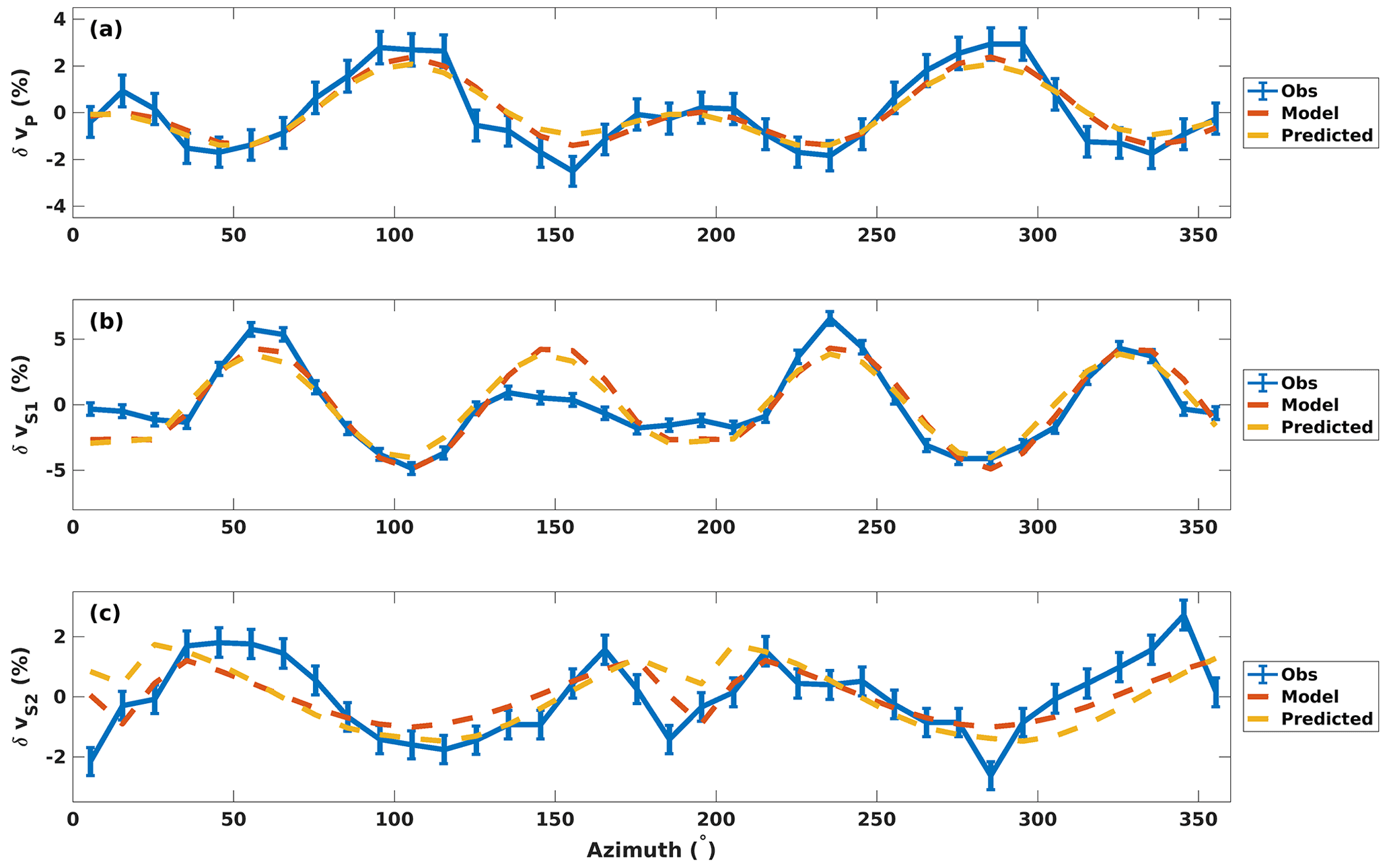
Figure 12 Observed, modelled and CPO-predicted anisotropy for sample 003. (a) δv_P; (b) δv_S1; (c) δv_S2.

The observed, modelled and forward-modelled velocity anisotropy for sample 007 is shown in Fig. 13. The observed anisotropy and model anisotropy are in excellent agreement, but both curves are clearly offset by $\sim \mathrm{10}{}^{\circ }$ from the predicted velocity variations from measured CPO in this sample.

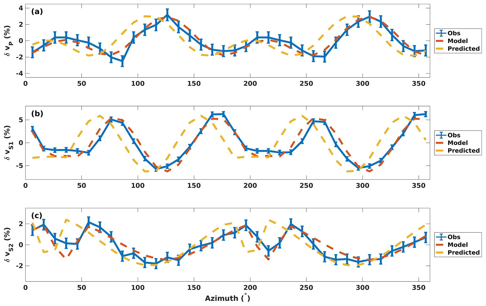
Figure 13 Observed, modelled and CPO-predicted anisotropy for sample 007. (a) δv_P; (b) δv_S1; (c) δv_S2.

This azimuthal difference between EBSD-measured CPO and CPO models based on ultrasonic data is best explained by small-scale variation within the samples. There is a potential azimuthal error of up to about 3^∘ in cutting and mounting samples for CPO measurement, and this error will primarily be a rotation around the core axis. Probably more important is the fact that the locations of CPO and ultrasonic measurements for a sample do not coincide. As small-scale rotations of the c-axis maximum, around a vertical axis, are observed in the core (Thomas et al., 2021), a difference in the sample position of a few centimetres along the core axis could give a few degrees rotation of the c-axis maxima. Some sample locations, through the depth of the core, have a population of oddly oriented grains, in addition to a main c-axis maximum (Thomas et al., 2021), that would give rise to a rotation around a vertical axis of sample-average acoustic anisotropy of $\sim \mathrm{10}{}^{\circ }$: areas with and without this orientation population can occur within the same core section (Fig. 9 in Thomas et al., 2021).

The seismic VSP data record wavelengths that are larger than the scale of individual samples and therefore do not resolve a variation in cluster orientation at this scale. The CPO model informed by VSP velocities provides an averaging of any given variation in CPO properties over the entire sampled depth range. The CPO model found to best explain the VSP data is characterised by a slightly larger cone opening angle compared to results of the individual ultrasonic measurements and therefore exhibits slightly weaker anisotropy.

5.2 The role of the studied seismic phase (P or S wave) and survey geometry on CPO model ambiguity

The VSP seismic and ultrasonic datasets presented in this study have fundamentally different acquisition geometries which ultimately determine the observed velocity variation due to CPO. The constraint of CPO models from seismic anisotropy is consequently highly sensitive to the sampling geometry.

The acquisition geometry of the VSP survey will have a critical control on the ability to distinguish different CPO patterns. For example the Flow and Perp lines show equally good P-wave (Fig. 8a, b) and S-wave (Fig. 9a, b) fits to the χ(v_P) model, which has the c-axis cluster azimuth at 65^∘ (Fig. 7a, Table 3), and to the χ(v_S1) and ∑χ models, which have the c-axis cluster azimuths of 110^∘ to 115^∘ (Fig. 7b, c; Table 3). The diagonal lines show clear differences in the predictions of the χ(v_P) model and the other models in both P-wave (Fig. 8c, d) and S-wave (Fig. 9c, d) velocity variations with the incidence angle. Modelling CPOs based on P-wave travel times alone does not give a good fit to the EBSD data on diagonal lines: using S-wave travel times or S-wave travel times combined with P-wave travel times gives a much better fit to the EBSD measurements.

The ultrasonic data offer a dense sampling of velocities along azimuths in the horizontal direction. The given CPO type with horizontal c-axis clusters exhibits the largest magnitude of velocity variation in the horizontal plane; therefore this sampling geometry results in high sensitivity to CPO parameters. The individual reconstructed CPO models using v_P, v_S1 or v_S2 anisotropy are found to be consistent and also generally agree with measured CPO in core samples (see Figs. 10 and 11). Periodicity of seismic anisotropy can result in ambiguities: δv_P and δv_S2 exhibit 180^∘ periodicity and reconstruct the CPO cluster's measured orientation without ambiguity. The cluster orientation reconstructed by χ(v_S1) is also found to agree with measured orientation; however a misfit local minimum, offset by a 90^∘ azimuth to the global misfit minimum, reduces confidence in the results. We suggest that it is important to consider the information from velocity measurements of all phases that are available to avoid a local minimum. In this study this is achieved by forming the sum of individual misfits χ and selecting the model associated with the misfit minimum in this case.

The influence of azimuthal sampling on model results is investigated by sub-sampling of the multi-azimuth ultrasonic dataset. Figure 14 presents model parameter results for sample 003 where, instead of 10^∘ azimuth spacing between measurements, increments of 20, 30, 60 and 90^∘ are used to inform CPO models. For each chosen new sampling interval, all possible downsampled datasets are considered. For example, an azimuth spacing of 20^∘ allows two downsampled datasets to be created: one, where the first measurement is taken at 0^∘ azimuth and another one, where the first measurement is at 10^∘.

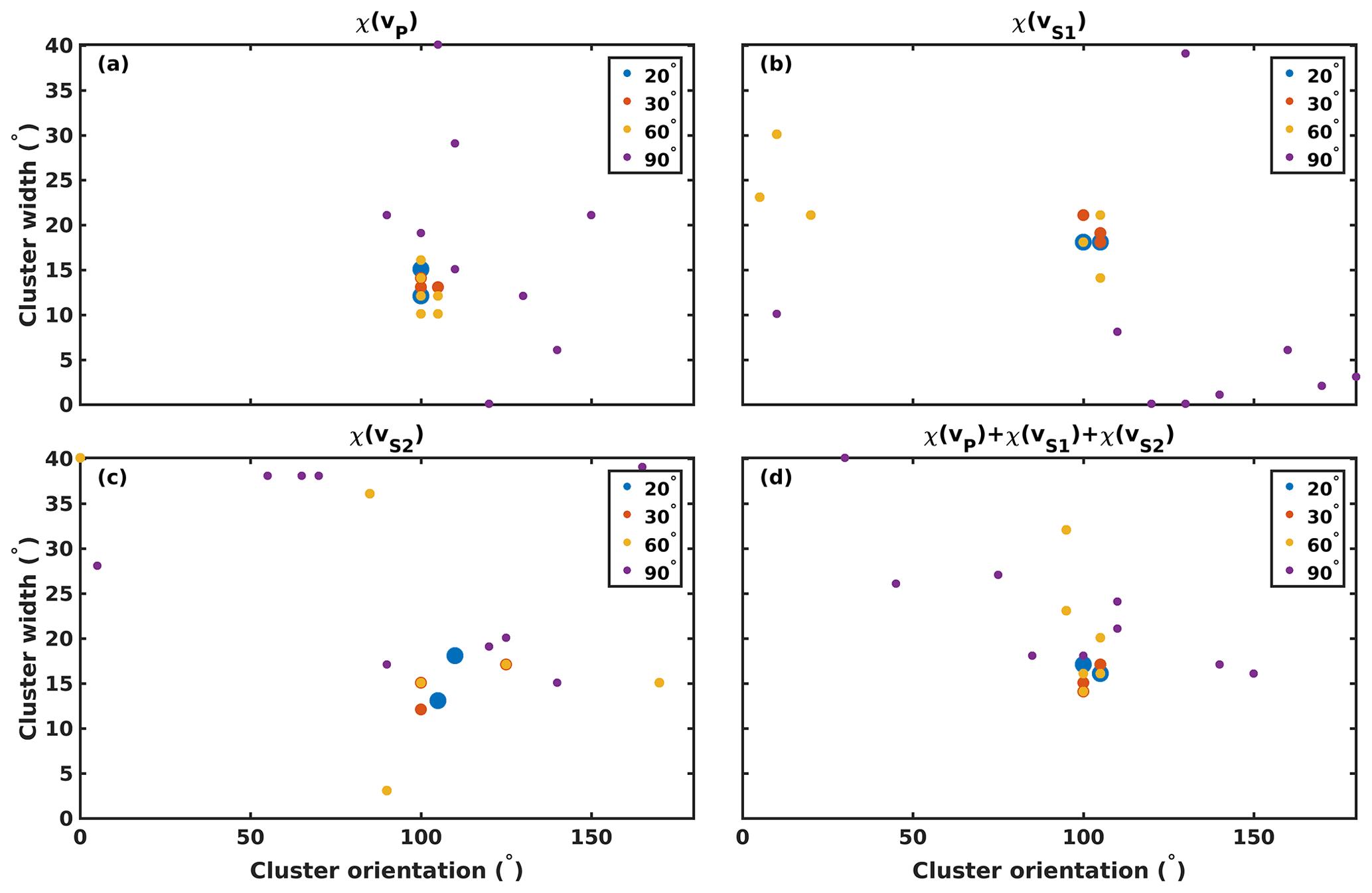
Figure 14 Parameter results using downsampled velocity measurements with azimuthal spacing of 20, 30, 60 and 90^∘ (indicated by symbol size) for sample 003: (a) χ(v_P), (b) χ(v_S1), (c) χ(v_S2) and (d) $\mathit{\chi }\left(v_{\mathrm{P}}\right)+\mathit{\chi }\left(v_{\mathrm{S}\mathrm{1}}\right)+\mathit{\chi }\left(v_{\mathrm{S}\mathrm{2}}\right)$.

Models informed by χ(v_P) (Fig. 14a) confirm the result of the full dataset if a coarser sampling of velocities with azimuth increments of 20, 30 or 60^∘ is chosen. Models informed by multi-azimuth measurements with 90^∘ spacing show a large spread of CPO parameter results. Models informed by χ(v_S1) and χ(v_S2) (Fig. 14b and c) agree for spacing of 20^∘ and 30^∘, with larger spacing resulting in a wide scatter of model parameters. At 60^∘ sampling, χ(v_S1) reconstructs three models at the EBSD-observed cluster orientation and three models at the 90^∘ offset orientation associated with the misfit local minimum in Fig. 10b. The approach of using the sum of all misfits (Fig. 14d) reduces the spread of the model parameters found and finds realistic models for 20 and 30^∘ spacing. For 60^∘ spacing, the cluster orientation angle is correctly found but the cluster width is poorly constrained. This is a clear improvement relative to the reconstructed model parameters in Fig. 14b and c for 60^∘ spacing. The results for 90^∘ spacing are widely scattered and not in agreement with the model parameters that were found using the full dataset. The discrepancy in model parameter results found by the different 90^∘ sampling geometry relates to the fact that there is more than one cluster orientation that will give the same ratios of orthogonal velocities. Thus the solution is very dependent on the measurement errors in the velocity dataset. At 90^∘ sampling the errors in v_S1 will be particularly influential as v_S1 velocities should be very similar for orthogonal azimuths (see predictions in Figs. 12 and 13).

Our downsampling analysis shows that in an ideal survey geometry, which is in this case given by the sampling of a horizontal-cluster CPO by horizontal velocity measurements, a realistic CPO model can be created from sampling in up to 30^∘ steps regardless of the seismic phase studied. Observed scatter in model parameter results shows that the set of actual sampled azimuths becomes critical for larger sampling intervals: the datasets with 20 and 30^∘ sampling are much less sensitive to the choice of the first sampled azimuth compared to the datasets with 60 and 90^∘ spacing. The consideration of the full range of seismic velocity information ($\mathit{\chi }\left(v_{\mathrm{P}}\right)+\mathit{\chi }\left(v_{\mathrm{S}\mathrm{1}}\right)+\mathit{\chi }\left(v_{\mathrm{S}\mathrm{2}}\right)$) can reduce scatter and aid in reconstructing a realistic CPO model from data with wider azimuthal spacing.

The VSP survey CPO modelling presents ambiguity in cluster orientation if only P-wave velocities are considered, as shown in Fig. 7a. The best-fitting model in this case does not match the CPO observations from the site, orienting the cluster at an azimuth that is offset by $\sim \mathrm{45}{}^{\circ }$ in the anticlockwise direction from observed cluster orientations. In Fig. 8 the uncertainties in δv_P observations are large compared to the P-wave anisotropy of the best-fitting model.

The difficulty in reconstructing a realistic CPO model from P-wave velocities in the VSP dataset is a consequence of poor azimuthal sampling. The VSP survey is characterised by coverage of ray paths from a range of incidence angles from multiple azimuths. For the given horizontal-cluster CPO this geometry is clearly not as sensitive to anisotropy as the dense azimuthal sampling of horizontal velocities, which characterises the ultrasonic measurements. The inclusion of P- and S-wave phase information mitigates this shortcoming of the VSP data by resolving the ambiguity in cluster orientation and identifying a CPO model which is in agreement with measured CPO. The study of all available seismic phases should therefore become standard in seismic CPO constraints in ice, rather than the commonly encountered focus on P-wave velocities.

For the horizontal-cluster CPO, the variation in seismic velocities with incidence angle is highly dependent on the azimuth. Therefore, VSP data might be unable to constrain this CPO if azimuths with strong variation are not sampled. The difficulty in finding a correct CPO model from VSP P-wave velocities could be a consequence of this problem, highlighted in Fig. 8 by large error bars relative to the overall v_P variation with incidence angle. A greater azimuthal sampling of VSP data is required to improve the CPO model constraint. Furthermore, larger shot offsets should be targeted to sample near-horizontal ray paths for the study of horizontal-cluster CPOs, since the largest amplitude of the anisotropy signal is in the horizontal plane.

6 Conclusions

We have conducted a vertical-seismic-profile (VSP) experiment and laboratory ultrasonic experiments aimed at measuring the seismic anisotropy of ice from the lateral shear margin of the Priestley Glacier, Antarctica, and at linking these data to seismic anisotropy model predictions based on measured crystallographic preferred orientations (CPOs) in EBSD data.

Horizontal-cluster CPO models are informed by P-wave and S-wave velocity anisotropy data from a ∼50 m scale, four-azimuth, walkaway-VSP experiment. A best-fitting CPO model informed by VSP P-wave data alone is found to exhibit a c-axis cluster azimuth, which is inconsistent with measured c-axis orientations and also overestimates the strength of c-axis clustering. Best-fitting CPO models based on VSP S-wave data or a combination of P-wave and S-wave data are found to give a good match to the direct CPO measurements.

Azimuthal ultrasonic P-wave and S-wave velocity measurements, made in 10^∘ increments, on core samples from the borehole show the pattern of anisotropy with considerable detail. The anisotropy pattern matches the pattern predicted from the CPO in the shallowest sample 003. Differences in CPO-predicted and measured anisotropy for deeper samples 007 and 010 are an indication of intra-sample CPO variability. Inter-sample variability is also apparent from ultrasonic velocity measurements: the anisotropy patterns in different samples are rotated through small angles relative to each other around the core axis, a pattern that matches direct CPO measurements.

The ultrasonic data have been downsampled to larger azimuthal increments (20, 30, 60 and 90^∘) to explore how well these lower-resolution data constrain the CPO responsible for velocity anisotropy. Increments of up to 30^∘ constrain both the azimuthal orientation and the intensity of horizontal c-axis alignment well. Increments of 60^∘ constrain orientation. Increments of 90^∘ do not provide useful constraints. The design of field seismic surveys should be designed to address ambiguity as result of sampling geometry by considering two main points. First, a dense sampling of propagation angles must be realised by the acquisition geometry. Second, sources and receivers must enable the derivation of both P-wave and S-wave anisotropy.