the Creative Commons Attribution 4.0 License.
the Creative Commons Attribution 4.0 License.
 | 03 Aug 2022
Surge dynamics of Shisper Glacier revealed by time-series correlation of optical satellite images and their utility to substantiate a generalized sliding law
Saif Aati
Ian Delaney
Surendra Adhikari
Jean-Philippe Avouac
Understanding fast ice flow is key to assessing the future of glaciers. Fast ice flow is controlled by sliding at the bed, yet that sliding is poorly understood. A growing number of studies show the relationship between sliding and basal shear stress transitions from an initially rate-strengthening behavior to a rate-independent or rate-weakening behavior. Studies that have tested a glacier sliding law with data remain rare. Surging glaciers, as we show in this study, can be used as a natural laboratory to inform sliding laws because a single glacier shows extreme velocity variations at a subannual timescale. The present study has two main goals: (1) we introduce a new workflow to produce velocity maps with a high spatiotemporal resolution from remote-sensing data, combining Sentinel-2 (S2) and Landsat 8 (L8) and using the results to describe the recent surge of Shisper Glacier, and (2) we present a generalized sliding law and substantiate the sliding-law behavior using the remote sensing dataset. The quality and spatiotemporal resolution of the velocity time series allow us to identify a gradual amplification of spring speed-up velocities in the 2 years leading up to the surge that started in November 2017. We also find that surface velocity patterns during the surge can be decomposed into three main phases, and each phase appears to be associated with hydraulic changes. Using this dataset, we are able to highlight the rate-independent and rate-weakening relationships between resistive stress and sliding during the surge. We then discuss the importance of the generalized sliding relationship to reconcile observations of fast ice flow, and in particular, different surge behaviors. The approach used in this study remains qualitative, but if coupled with better bed-elevation data and numerical modeling could lead to the widespread quantification of sliding-law parameters.
- Article
(14390 KB) - Full-text XML
-
Supplement
(3186 KB) - BibTeX
- EndNote


Describing the physics of glacier basal motion is a core challenge in modern glaciology. Enhanced basal motion can lead to the demise of large ice shelves, and would lead to rapid and significant sea-level rise (e.g., Mouginot et al., 2019; Catania et al., 2020; Pattyn and Morlighem, 2020). Sliding-dominated ice flow at tidewater glaciers is responsible for the majority of mass loss from the Greenland Ice Sheet (e.g., Mouginot et al., 2019) because the ice advected into the ocean facilitates calving and melting. Glacier surges can show velocities reaching tens of kilometers per year (e.g., Hewitt, 1969; Meier and Post, 1969; Post, 1969; Kamb et al., 1985), which redistribute ice mass dramatically, and can lead to enhanced ice loss, disturbed glacial runoff, and can create multiple hazards for local communities (e.g., Hewitt and Liu, 2010; Bhambri et al., 2020). Large sliding-dominated ice flow velocities cannot generally be explained by traditional Weertman-type sliding relationships (e.g., Lliboutry, 1968; Iken, 1981; Tulaczyk et al., 2000; Iverson and Iverson, 2001; Schoof, 2005; Zoet and Iverson, 2015; Minchew et al., 2016; Stearns and Van der Veen, 2018; Zoet and Iverson, 2020) that express the basal shear stress as proportional to the sliding velocity (Weertman, 1972; Budd et al., 1979; Bindschadler, 1983, see also Fig. 1).
The idea that bed shear stress is bounded for large sliding velocities was proposed in early physical glaciology work (Lliboutry, 1968; Iken, 1981). However, this idea only started to gain more traction in the early 2000s (Tulaczyk et al., 2000; Iverson and Iverson, 2001; Schoof, 2005). Since then, a growing body of research on the mechanics of glacier sliding has arisen (Tulaczyk et al., 2000; Iverson and Iverson, 2001; Schoof, 2005; Gagliardini et al., 2007; Iverson, 2010; Pimentel and Flowers, 2010; Iverson and Zoet, 2015; Tsai et al., 2015; Zoet and Iverson, 2015; Minchew et al., 2016; Joughin et al., 2019; Zoet and Iverson, 2020), proposing new relationships between shear stress and sliding velocity. These relationships can generally be partitioned into three regimes (Fig. 1; see also Minchew and Joughin, 2020): (1) form drag, similar to Weertman-type relationships, where drag is dominated by viscous deformation of ice around bed obstacles, and shear stress increases monotonically with sliding velocity, (2) a transition regime, where shear stress approaches or even reaches its maximum value and starts decreasing, and (3) skin drag, where drag becomes dominated by the friction between ice and the bed, and shear stress reaches an asymptote (i.e., Coulomb failure; Tulaczyk et al., 2000; Iverson and Iverson, 2001; Iverson, 2010) or decreases monotonically with sliding velocity (Fig. 1; Schoof, 2005; Gagliardini et al., 2007; Zoet and Iverson, 2015).
While these theories represent the physics of ice sliding better than their Weertman-type predecessors, they currently suffer from a number of caveats that prevent testing them in the real world and using them in numerical simulations (Pimentel and Flowers, 2010; Jay-Allemand et al., 2011; Beaud et al., 2014; Tsai et al., 2015; Joughin et al., 2019; Thøgersen et al., 2019). These caveats include the following: (1) one has to choose between a slip relationship suited for a rigid non-deformable bed, i.e., bedrock, or for a deformable bed, i.e., sediment, (2) tuning the parameters requires knowledge of small-scale bed properties (e.g., sediment characteristics, bed geometry), and (3) the possibility of non-unique solutions renders numerical solving challenging (Pimentel and Flowers, 2010).
Surge-type glaciers undergo cyclic switches in their flow regime between slower-than-normal (quiescence) and faster-than-normal (surge) velocities (Meier and Post, 1969). During quiescence, the glacier builds up ice mass in a reservoir area where the resistance to ice flow exceeds the driving stress (Cuffey and Paterson, 2010). The surge occurs when the driving stress exceeds the resistive stress, and glacier velocities increase by typically 1 order of magnitude in comparison with quiescence velocities. This local and dramatic velocity increase creates an ice bulge that travels down the glacier as a kinematic wave (e.g., Kamb et al., 1985; Mayer et al., 2011; Adhikari et al., 2017). If the ice-mass redistribution is significant enough, the terminus of the glacier will become the receiving area, thicken, and may start advancing. Surge-type glaciers only represent about 1 % of glaciers worldwide (Jiskoot et al., 2000), and appear to be concentrated in climatic clusters (e.g., Sevestre and Benn, 2015). A recent theory for glacier surges suggests that a specific combination of climatic conditions is required to create an unstable equilibrium in surge-type glaciers, based on coupled mass and enthalpy budgets approach (Benn et al., 2019).
Surge-type glaciers can be used to assess how basal shear stress depends on sliding velocity. Surges are dynamic instabilities during which surface velocities increase at least 10-fold, and have return periods typically between a decade and a century (Meier and Post, 1969; Clarke et al., 1986; Jiskoot et al., 2000; Jiskoot, 2011; Quincey et al., 2011; Sevestre and Benn, 2015). The back and forth oscillation between relatively low and high velocities for a single glacier makes it possible to test the temporal transition between different sliding regimes. Seasonal velocity fluctuations can also be used in principle to test friction laws, although their duration is relatively short (typically a few weeks) and their amplitude relatively low (typically 20 %–50 % velocity increase), thus requiring particularly high resolution and quality data.
Satellite imagery is a valuable source of information to study glacier dynamics. It allows monitoring with a large spatial coverage and metric ground resolution, including otherwise inaccessible areas (e.g., Burgess et al., 2013; Quincey et al., 2015; Armstrong et al., 2017; Gardner et al., 2019; Dehecq et al., 2019). The temporal resolution of remote sensing is however limited by the time span between the acquisition of two images, often weeks to months, necessary to create a displacement map. Glacier velocities derived from remote sensing will therefore consistently miss sub-monthly fluctuations, in particular those at the daily or subdaily timescales which can be significant (e.g., Kamb et al., 1985; Iken and Bindschadler, 1986; Iken and Truffer, 1997). Advances in algorithms to model, register, and correlate optical images with a subpixel accuracy (e.g., COSI-Corr, MicMac, ASP, CIAS, Medicis; see Rupnik et al., 2017; Rosu et al., 2015; Beyer et al., 2018; Heid and Kääb, 2012), combined with the ever-growing volume of satellite remote-sensing datasets available (e.g., Gardner et al., 2019), nonetheless provide opportunities for glaciology studies. Remote sensing has thus offered insight into recent surges (e.g., Copland et al., 2011; Dunse et al., 2015; Round et al., 2017; Steiner et al., 2018; Chundley and Willis, 2019; Rashid et al., 2019; Bhambri et al., 2020; Paul, 2020), as well as multiannual glacier dynamics (Moon et al., 2014; Van de Wal et al., 2015; King et al., 2018) and basal sliding mechanisms (Minchew et al., 2016; Stearns and Van der Veen, 2018). In this paper, we apply image correlation to a time series of optical images using COSI-Corr (Leprince et al., 2007), which is accurate to 1/20th of the pixel size, and we use a post-processing method based on a principal component analysis (PCA) to measure spatiotemporal variations of ice velocity. This method is applied to openly-available Landsat 8 (L8) and Sentinel-2 (S2) optical images of two surge-type glaciers in Pakistan's Karakoram, Himalaya. We retrieve a time series of velocity maps with 60 m pixels and a temporal resolution as low as 5 d over 6 years from 2013 to 2019. We additionally use commercial optical images to create digital elevation models (DEMs) and constrain ice volume changes during the surge (Aati and Avouac, 2020).
Of the two neighboring surge-type glaciers, Shisper Glacier (Fig. 2) experienced a dramatic surge during the study period, which saw its terminus advance by ∼1.7 km (Rashid et al., 2019; Bhambri et al., 2020). Over that period, the other glacier, Mochowar (Fig. 2), appears to have remained stable. Given the lack of local weather data, we use Mochowar as a reference glacier that we assume reflects the ice flow response to local climate in the absence of a surge.
This paper is composed of four parts: (1) we show that rigid and deformable bed theories can be combined into a generalized sliding relationship applicable for any glacier environment and dynamic evolution; (2) we present the remote sensing method and workflow; (3) we apply this workflow to Shisper and Mochowar glaciers and characterize the surge of Shisper Glacier; and (4) we use the dataset for Shisper Glacier to substantiate the generalized sliding relationship and contextualize how this theory can improve our understanding of surge dynamics, and more generally, basal sliding.
The early work of Weertman (1957) relating glacier sliding, ub, over a rigid idealized bed to basal shear stress as τb∝ub, set the standard for generations of glaciologists, and remains relevant (MacAyeal, 2019). This formulation, which was later modified to allow for a nonlinear behavior, (Weertman, 1972), and for a dependence on effective pressure, N, (Budd et al., 1979; Bindschadler, 1983), remains most widely used (e.g., Cuffey and Paterson, 2010). We will hereafter refer to this type of relationship as Weertman-type.
The bed of a glacier can only produce a finite amount of resistance to flow that is determined by its properties (e.g., Lliboutry, 1968; Iken, 1981; Tulaczyk et al., 2000; Iverson and Iverson, 2001; Schoof, 2005), challenging the validity of Weertman-type relationships which imply an unbounded resistance to flow. For bedrock, i.e., a rigid bed, that limit is dictated by the maximum adverse slope of bedrock obstacle to flow in contact with the ice (Lliboutry, 1968; Iken, 1981; Schoof, 2005; Gagliardini et al., 2007; Zoet and Iverson, 2015). For till, i.e., a deformable bed, that limit is dictated by the shear resistance of the material (Tulaczyk et al., 2000; Iverson and Iverson, 2001; Iverson, 2010; Zoet and Iverson, 2020). As a consequence, past a velocity threshold, the shear stress tends to an asymptotic value or reaches a maximum and eventually decreases, while the sliding velocity increases (Fig. 1a). That decrease can be the result of bed-weakening feedbacks at high velocities. For a deformable bed, it could be associated with reworking of the till matrix and a change in its geotechnical properties (e.g., Clarke, 2005). For a rigid bed, the maximum adverse slope to flow can be engulfed in basal cavities as they grow (Fig. 1d and f). In short, the relationship between basal sliding and shear stress is dominated by form drag as velocities remain below some threshold velocity. For sliding velocities slightly above that threshold, there is a transition regime where form drag and skin drag are competing. Beyond that regime, skin drag becomes dominant and sliding can continue to increase while shear stress reaches an asymptotic value or decreases (Fig. 1a, f and g).
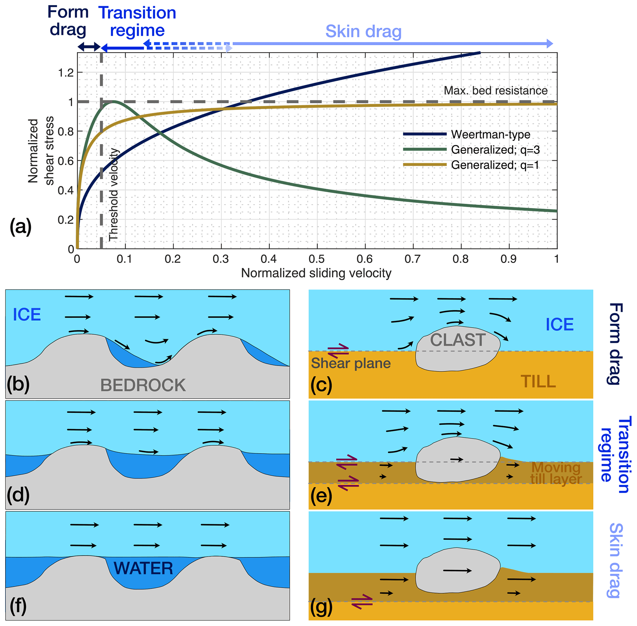
Figure 1Conceptual representation of glacier sliding relationships for rigid and deformable beds, inspired by Minchew and Joughin (2020). Plot of normalized shear stress versus normalized sliding velocity, comparing Weertman-type sliding and two forms of the generalized sliding relationship (a). Schematic representation of form drag (b, c), transition regime (d, e), and skin drag (f, g) for a rigid bedrock bed (b, d, f) and for a deformable till bed (c, e, g). We use form drag to describe the macroscopic viscous drag on bed obstacles and skin drag to describe the viscous drag at the scale of the boundary layer between the ice (fluid) and bed. The transition regime depends on the bed characteristics (in particular q), and the shift to skin drag can be arbitrary. It is different for each relationship plotted, hence the dashed lines showing the possible overlap. For a rigid bed, the skin friction regime can be likened to a curling stone sliding on an ice track, while it represents Coulomb failure for a deformable bed. Note that the shear stress is normalized by an imposed , and the sliding velocity normalized arbitrarily by 40 m d−1, , and p=3. For the Weertman-type relationship, we use , with , and .
The relationships between sliding and shear stress for rigid and deformable beds show similar patterns, yet are the result of fundamentally different physical processes. We show that the two sliding relationships can be unified and expressed using a general glacier sliding relationship. The rigid-bed sliding relationship first proposed by Schoof (2005) and generalized by Gagliardini et al. (2007) is
where τb is the basal shear stress, C is a parameter that sets the maximum friction-law value, i.e., that remains smaller or equal to the maximum slope of obstacles on a rigid bed (Gagliardini et al., 2007), is the effective pressure at the glacier bed defined as the difference between overburden ice and water pressures, χ is a normalized velocity, p is power-law exponent, and q is an empirical exponent that relates to the strain weakening of the bed. Note that q should be greater than, or equal to 1, and that the relationship is rate-independent if q=1, and rate-weakening if q>1. The term α is defined as so that the maximum of τb is CN, and χ is defined as
The term ub is the sliding velocity and As is a sliding parameter without cavity. Note that CpNpAs has the dimension of a velocity. Zoet and Iverson (2020) propose the following sliding relationship for a deformable bed:
where ϕ is the friction angle of the till, and ut is a threshold sliding velocity above which till resistance is defined by its Coulomb strength. The sliding relationships for rigid (Eq. 1) and deformable (Eq. 3) beds can be reconciled by defining two bed-dependent variables. First, we define a maximum resistive stress σmax as
then we generalize the threshold velocity:
where Cd is a spatially variable parameter accounting for till properties. This leads to the generalized sliding relationship:
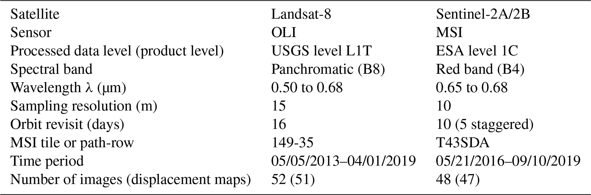
Table 1Overview of satellite data products analyzed in this study.
From Eqs. (4)–(6), N stands out as the variable responsible for temporal changes in σmax and ut. The other parameters (C, As, Cd and ϕ) have been shown to change spatially (Gagliardini et al., 2007; Zoet and Iverson, 2020) but are not expected to vary significantly over time spans relevant for a glacier surge, i.e., a decade. The fact that N is raised to the power p>1 in Eq. (5), however, precludes from writing Eq. (6) for the general case explicitly as a function of N. This highlights the variables of interest to use the generalized relationship in data inversion efforts, or to refine rate-and-state approaches (e.g., Thøgersen et al., 2019). It can complicate the use of the relationship in numerical models where the direct use of N might be necessary, although existing models that readily solve for water pressure, and thus calculate N, will already have chosen a type of substrate as dictated by water flow in different media (see Flowers, 2015, for a review). Note that for a deformable bed, substituting Eqs. (4) and (5) into Eq. (6) and setting q=1, simplifies Eq. (3). We use the general law expressed by Eq. (6) in our analysis.
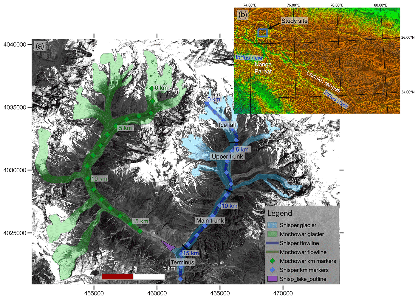
Figure 2Overview of the study area. (a) Outlines of Mochowar (green) and Shisper (blue) glaciers with the location of the median flowlines used for analysis, and the maximum extent of the periglacial lake, overlaid on the Sentinel-2 optical image from 15 July 2018. The labels on Shisper glacier describe four zones identified as undergoing different dynamic processes during the surge. The icefall zone spans across the accumulation and ablation area of Shisper glaciers where surface slopes are steep (up to 45∘) and elevation >3750 m a.s.l. The upper trunk is within the ablation area and is where four tributaries merge with the main glacier. Surface elevations are comprised between 3750 and 3400 m a.s.l., and the zone terminates just downflow from the last identifiable icefall along the profile. The main trunk is characterized by relatively uniform surface slope with no icefall or tributary junction and surface elevations range from 3400 and 2750 m a.s.l. The terminus zone is below 2750 m a.s.l. and represents the area that shows dynamic activity almost only linked to the advancing surge bulge. Coordinates are in meters and projected on zone 43 N of the Universal Transverse Mercator (UTM) coordinate system. (b) Relief map of the Western Himalayan and Karakoram regions with notable geographic features for reference.
3.1 Study area
Shisper and Mochowar glaciers are located in the Hunza Valley, in the Karakoram region in northwestern Pakistan (Fig. 2). The Karakoram region shows a high concentration of surge-type glaciers (e.g., Hewitt, 1969; Sevestre and Benn, 2015), with approximately 90 such glaciers documented (Copland et al., 2011). A climatic anomaly allows glaciers in the Karakoram region to maintain their ice volume (e.g., Hewitt, 2005; Gardelle et al., 2012; Kääb et al., 2015; Farinotti et al., 2020). Shisper and Mochowar glaciers occupy adjacent valleys connecting as a Y, and were merged until 2005. They are denominated as a single entity, Hassanabad Glacier, in the Randolph Glacier Inventory (Pfeffer et al., 2014). The relief in the area is dramatic as the elevation drop between the Shispare Peak (7611 m a.s.l.) and Shisper Glacier terminus (2500 m a.s.l.) is larger than 5000 m across 15 km. The glacier bergshrunds are perched between ∼5000 and ∼5500 m a.s.l., suggesting that the relief of each glacier is greater than 2000 m. The glaciers we refer to as Shisper and Mochowar (Rashid et al., 2019), have also respectively been referred to as Shispare and Muchuhar (Bhambri et al., 2020), or Shishper and Muchowar (Karim et al., 2020).
Bhambri et al. (2017) identified surges of Shisper Glacier in 1904–1905, 1972–1976, and 2000–2001, although inspection of Landsat images suggests that the last advance of Shisper Glacier ended in 2005 (see Sect. S3 in the Supplement). A line of evidence indicating a past surge of Mochowar Glacier is the disintegration of 3.6 km of its terminus in ∼10 years, starting in 2005, suggesting that it was stagnant ice left from a prior advance. Melt from both glaciers feed a hydroelectric power plant in the Hunza Valley and glacier-related hazards threaten the town of Hassanabad and the Karakoram Highway, which is the only paved road crossing the mountain range (Shah et al., 2019; Rashid et al., 2019; Bhambri et al., 2020).
3.2 Dataset
We use data from the L8 (United States Geological Survey, USGS) and S2 (European Space Agency, ESA) optical satellite systems to determine glacier surface velocities from May 2013 to August 2019. The two imaging systems have similar spectral properties, ground resolution, acquisition rate (Table 1), and the data are free and open access (Roy et al., 2014; Drusch et al., 2012). We utilize all images with less than 20 % cloud cover over the study area, yielding a total of 100 images: 52 images acquired from L8 between 5 May 2013 and 1 April 2019, and 48 images from S2 between 21 May 2016 and 9 August 2019 (see Table S2.1 in the Supplement).
Two satellites comprise the S2 constellation, i.e., S2A and S2B. Both use the same multispectral instrument (MSI) sensor (Table 1) and have a return time of 10 d, producing a staggered return interval of 5 d. The S2B was launched later than S2A, and the first usable image from that satellite is in November 2017. Of the 48 S2 images, 25 images were acquired from the S2A sensor and 23 images were taken from the S2B sensor. The S2 data products were downloaded from the Sentinel Open Access Hub platform (ESA, 2019) in the Universal Transverse Mercator (UTM) zone 43N projection coordinate system as a Level-1C tile (100 km ×100 km). The Level 1C product level consists of ortho-images, radiometrically corrected top-of-atmosphere reflectance values, and geometrically corrected based on a refined geometric model. We used the red band (band 4) of S2 because it is appropriate for glacier monitoring (Kääb et al., 2016) and used as a reference for band-to-band coregistration (Table 1; Gascon et al., 2017).
The L8 utilizes the Operational Land Imager (OLI) sensor, with a swath width of 185 km (Table 1), and has a 16 d temporal resolution. We downloaded L8 images from the Earth Explorer platform of USGS (U.S. Geological Survey, 2019) as L8 L1T products. The processing of L8 products is similar to that of S2 data with respect to radiometric and geometric corrections, orthorectification, and re-sampling to a map grid. We chose the L8 panchromatic band (band 8), due to its 15 m spatial resolution, (Table 1). All available optical images were used to map the evolution of the paraglacial lake and terminus advance.
We used the Shuttle Radar Topography Model (SRTM, U.S. Geological Survey, 2014) DEM in combination with three DEMs, one in 2017 and two in 2019, that were calculated with Planetscope, GeoEye-1 and WorldView-2 images as presented by Aati and Avouac (2020). To constrain the bed topography of Shisper Glacier, we use the data products from Farinotti et al. (2019). For Shisper Glacier, the ice thickness was estimated as the composite of three different models, as detailed in Farinotti et al. (2017). The specific DEM used is a combination of ASTER and SRTM DEMs (NASA/METI/AIST/Japan Spacesystems and U.S./Japan ASTER Science Team, 2018; U.S. Geological Survey, 2014) for which the timing of acquisition is not specifically known. It is likely in the mid-2000s, after the last surge of Shisper Glacier.
The data processing consists of three main steps (processing chain in Fig. 3) which we detail in the following subsections and in the supplement. (a) The data is prepared by clipping the images to the study area, and removing the cloudy images. (b) Surface displacement maps are calculated from correlating consecutive images with the COSI-Corr software package (Leprince et al., 2007). For each image pair there are three outputs, east–west and north–south displacement maps and a map of signal-to-noise ratio (SNR). (c) The data is filtered and artifacts removed, for example systematic offset between sensors. The processing chain was designed to allow for a nearly automated processing of all the available data (L8 and S2).
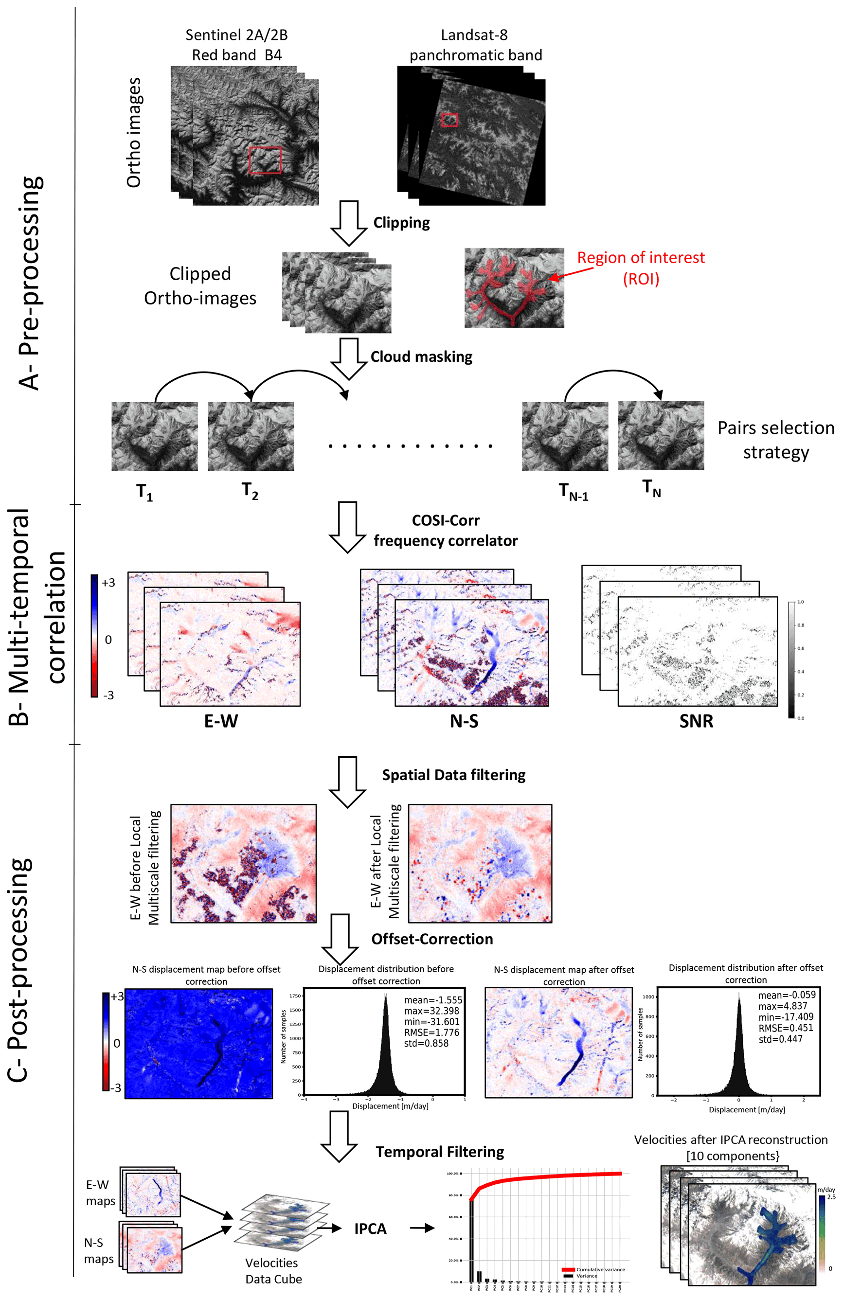
Figure 3Workflow for image processing, displacement map preparation, and velocity map post-processing.
Until the post-processing (step C, Fig. 3), images are processed independently for either satellite. The correlation of S2 and L8 images are not included due to systematic orthorectification artifacts. The USGS and ESA only release ortho-images and we would need access to non-rectified images in order to circumvent these artifacts. We only use pairs with the smallest consecutive time span for the correlation, which leads to a sequence of n−1 displacement maps for each satellite with n different acquisition dates. This strategy was chosen so as to get a complete times series for a minimal computational volume.
4.1 Image pairs correlation
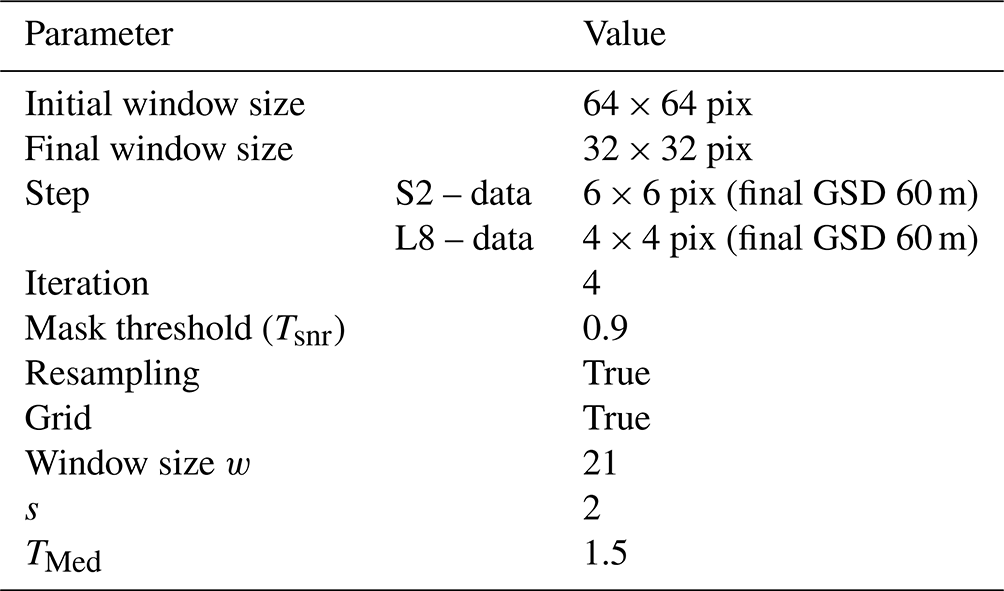
This study implements the COSI-Corr frequency correlator (Leprince et al., 2007), which is better adapted to measure small displacement over short time spans than the statistical correlators included in other image correlation packages (e.g., MicMac, CIAS, Medicis; see Heid and Kääb, 2012; Rosu et al., 2015). This correlator works in two processing steps. (1) The first step provides a coarse estimate using a large sliding window. (2) A subpixel accuracy is obtained from a second correlation using a smaller window. Three parameters are chosen: the step which determines the spatial resolution of the displacement map and the sizes of the first and second sliding windows. The values used in this study are listed in Table 2. With these parameters we obtain independent measurements of surface velocities with a ground resolution of about half the size of the smaller window, i.e., 160 m for S2 and 240 m for L8. Our velocity maps, which have a pixel size of 60 m, are thus oversampled by a factor 3 (S2) or 4 (L8). The image correlation process yields two displacement maps, each representing one of the horizontal displacements (east–west and north–south), as well as a measure of the correlation quality (e.g., SNR). The proposed workflow does not depend on the choice of a particular image correlation algorithm and can be based on any other image correlation software.
Table 2Summary of the parameters used for image correlation and displacement filtering.
4.2 Filtering and registration improvement
After the image pair correlation, three post-processing steps take place: (1) spatial data filtering to remove outliers from each displacement map and fill in missing data, (2) offset correction, to reduce systematic offsets due to incorrect orthorectification, and (3) reduction of noise level using PCA. This noise reduction takes advantage of the correlations in space of the displacement field.
To perform the spatial data filtering and data filling, we designed a specific multiscale spatial filtering process to remove erroneous measurements due to clouds, snow cover or surface water. This post-correlation tool, entitled Local Multiscale Filter (to be included in forthcoming version of COSI-Corr), consists of four steps (Appendix A):
-
Step 1. Filtering outliers with high uncertainty. We exclude measurements with low SNR by removing measurements with either (1) an SNR value smaller than a certain threshold Tsnr or (2) outliers beyond a user-selected multiple of the standard deviation (Tσ).
-
Step 2. Weighting of each displacement map with SNR.
-
Step 3. Filtering outlier displacement measurements. For each displacement measurement of the correlation map in position (x,y), we define a neighborhood window , where the s parameter is user-defined and controls the size of the window. Then, the algorithm removes values larger than TMed×Med, where Med is the median value of the displacement measurement in w, and TMed is a user-defined threshold, taken as TMed=1.5 here. To avoid filtering out reliable local values, a validation process is applied for each w, where the window is only considered valid if at least 70 % of the values lie within the confidence interval defined by , where denotes the absolute value. Otherwise, the window scale changes depending on the scale factor setting f.
-
Step 4. Filling in missing data. We estimate the missing values created during the steps above. The algorithm flags filtered values as missing data (e.g., NaNs) in defining an uncertainty matrix. For each window, NaN values are initiated by the Med value of window w, and the weight of this measurement is defined as the mean of SNR values in the neighboring window w. Otherwise, the original displacement value weight remains consistent with the original SNR value. This step relies on the assumption of local spatial coherence across neighboring windows w, i.e., that the displacement changes gradually rather than abruptly.
After the spatial filtering, we apply a correction for the offsets caused by the misregistration of available data products. These errors can be mitigated by optimizing the coregistration of the images during the orthorectification procedure (e.g., Avouac and Leprince, 2015). However, accounting for misregistration is not possible with S2 and L8 data, and we simply apply a linear correction to the correlation maps which provides a first-order systematic correction.
The final step consists of filtering the data. This step relies on the assumption that the spatial pattern of surface velocity is highly correlated. Spatial ice flow variations occur at a scale much larger than the ground sampling distance of our velocity maps. To identify these correlations, we use PCA and reconstruct displacement maps with the limited number of components needed to recover the data variance. This process reduces the noise level while preserving the inherent spatial resolution of the data. We retain the k first components needed to account for 90 % of the variance. We convert the displacement maps to surface velocities by dividing the elapsed time between the paired images.
Velocity maps are stacked on the same data cube D based on the older image date. When velocity maps overlap, we use the velocity map with the older starting image for the time span of the overlap. The data cube is then decomposed into principal components. This procedure does not involve any smoothing of the temporal variations of ice velocities. Abrupt variations affecting a limited area are however filtered out, because they would not contribute significantly to the data variance.

Figure 4Velocity maps showing the dynamic behavior of Mochowar and Shisper glaciers between 2013 and 2019. (a) Quiescence in the absence of seasonal speed-up; (b) spring speed-up; (c) fall speed-up; (d) enhanced velocities during spring speed-up in 2016; (e) enhanced velocities during spring speed-up in 2017; (f) slow fall onset of the surge; (g) phase 1 of the surge; (h) phase 2 of the surge; (i) phase 2 of the surge after lake formation; (j) phase 3 of the surge. The choice of velocity snapshot is aimed at displaying the most notable velocity patterns of Shisper Glacier, while Mochowar Glacier is used as a reference. Note that the velocity map for each glacier is not always taken over the exact same time period in order to display the cleanest velocity maps, in which case, the time stamp is shown in purple for Mochowar Glacier and blue for Shisper Glacier. The color bars have different scales for either glacier to better display velocity patterns. Perceptually uniform color maps are used in this figure to prevent visual distortion of the data (Crameri, 2018a, b).
5.1 Result overview
We present the surface velocities of the two glaciers together to allow for a relative comparison (Fig. 4). Mochowar Glacier only shows relatively regular seasonal variations (see Figs. S3.1 and S3.2). Shisper Glacier shows much more variability and we can distinguish various patterns: (1) relatively slow velocities during the quiescence and between speed-ups (Fig. 4a), (2) spring speed-ups (Fig. 4b, d and e; see also Abe and Furuya, 2015), (3) fall speed-up (Fig. 4c), (4) surge onset (Fig. 4f), and (5) different phases of the surge (Fig. 4g, h, i and j). Spring speed-ups are seen clearly in both glaciers, but the other forms of velocity patterns are unique to Shisper Glacier.
During the quiescence, velocities are generally comprised between ∼0.35 and in the upper and main trunks. Surface velocities during the spring speed-ups increase in amplitude from in the main trunk in 2015 (Fig. 4b), to in spring 2016 (Fig. 4d), and to in spring 2017 (Fig. 4e), eventually leading up to the surge onset by the end of 2017 (Fig. 4f). As the surge starts, velocities are consistently greater than in the lower part of the upper trunk and below. Before the surge onset, we can distinguish seasonal speed-ups in the fall (Fig. 4c), showing velocities greater than throughout the main trunk. The timing of these fall speed-ups correlates well with that of the onset of the surge in 2017 (Fig. 4f).
Phase 1 of the surge displays velocities greater than 1 m d−1 over most of the glacier with the entire main trunk flowing faster than 6 m d−1 (Fig. 4g). Phase 2 is characterized by significantly slower velocities, yet the main trunk keeps on flowing at 1 m d−1 at least, with a maximum above 3 m d−1 towards the terminus (Fig. 4h). An interesting event during phase 2 is the formation of a paraglacial lake once Shisper Glacier blocks the valley from Mochowar Glacier (mid-November 2018). The lake filling is associated with a short-lived increase in surface velocities () in the lower main trunk and terminus area (Fig. 4i). Finally, phase 3 shows very similar velocity patterns to phase 1 (Fig. 4j), with most of the glacier flowing faster than 1 m d−1, and the main trunk flowing faster than 7 m d−1. In addition, terminus velocities are greater than 3 m d−1 as the surge bulge progresses.
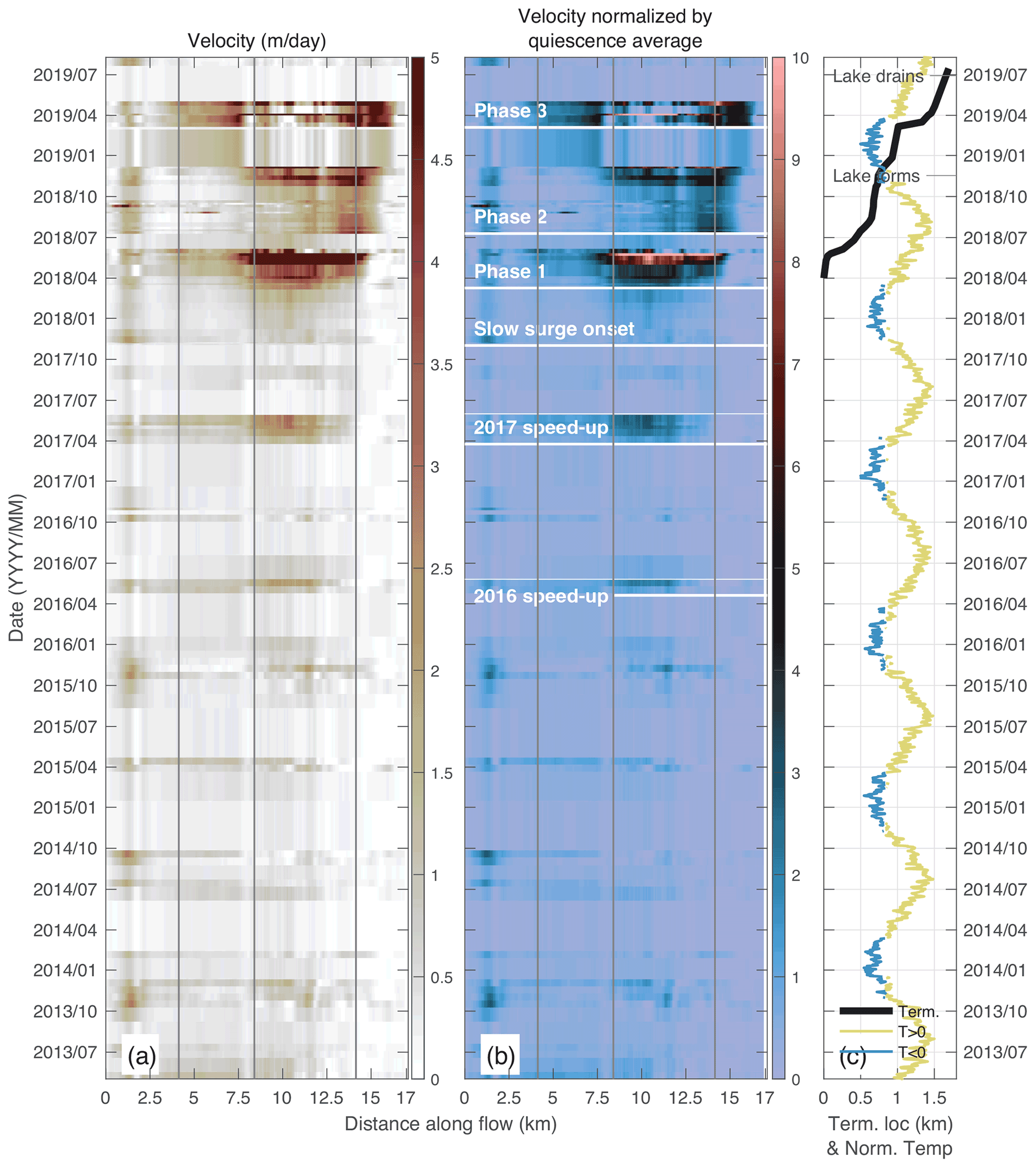
Figure 5Time series of (a) surface velocity and (b) normalized surface velocity along the flowline of Shisper Glacier (Fig. 2) from 2013 to 2019. The plots were produced from the data cube of L8 and S2 images with the PCA reconstruction. (c) Time series of terminus position advance and MERRA-2 satellite reanalysis of mean daily temperature at the mean elevation of the main trunk for the study area and for the plotting temperature are normalized by the maximum value. Blue and yellow represents temperature below and above 0∘, respectively. In (b) velocities are normalized with respect to average surface velocity during the quiescence (). Normalized velocities exceeding 10 are considered surge velocities. The vertical lines delineate the different regions of the glacier, and the major surface velocity patterns that we identified are shown with the horizontal labeled white lines. Perceptually uniform color maps are used in this figure to prevent visual distortion of the data (Crameri, 2018a, b).
5.2 Shisper Glacier surge and its build-up
The surface velocities of Shisper Glacier exhibit a marked seasonal pattern from the beginning of the time series and throughout the surge (Fig. 5a). This seasonal signal prior to the surge consists of surface velocities exceeding 1 m d−1 for a significant portion of the glacier profile, compared with velocities remaining between ∼0.35 and otherwise. This seasonality is expressed, biannually, between March and June, i.e., a spring speed-up, and another velocity increase between late September and November, that we will hereafter call fall speed-up. It appears that the presence of snow introduces a significant amount of noise in the data between fall and winter, especially at high elevations, i.e., between kilometers 0 and 2 along the profile. The fall speed-up is clear in 2013 and 2015, faint but present in 2016, and our results are inconclusive for 2014.
In the absence of field measurements, we use the temperature reanalysis data from the Modern-Era Retrospective Analysis for Research and Applications, version 2 (MERRA-2; Gelaro et al., 2017) to confirm that this seasonality is linked with glacier surface melt, and thus hydrology (Fig. 5c). The spring speed-ups occur soon after the daily-averaged temperature at 2 m. a.g.l. is estimated to exceed 0 ∘C at the mean elevation of the main trunk. The main trunk is located at least 1 km below this elevation, which suggests that it is undergoing significant surface melt. Similarly, the fall speed-ups occur soon after the reanalysis temperature at 4176 m. a.s.l. drops below freezing, hence when water supply from the glacier surface is expected to be shutting off and the drainage system of the glacier is shutting down.
Defining a surge based on surface velocities is somewhat arbitrary. A criterion that is pervasive in the literature is that surface velocities increase by 1 order of magnitude during the surge (e.g., Clarke et al., 1986), compared to that during the quiescence. Thus, we normalize surface velocities by the average of velocity during the quiescence, i.e., from the beginning of the time series until the slow onset of the surge in November 2017 (Fig. 5b). We consider that when normalized velocities reach or exceed 10, surge-level velocities are reached. This normalization further highlights the gradual increase in the amplitude of the spring speed-up as the surge becomes more imminent. In 2016, the speed-up shows velocities that are 5- to 6-fold the average quiescence velocities, and in 2017 the 10-fold threshold is reached (Fig. 5b). Aside from the spring speed-ups in 2016 and 2017, surface velocities seldom exceed before the surge onset, which is similar to surface velocities at Mochowar Glacier. Note that the highest velocities are located in the main trunk region of the glacier.
In November 2017, velocities increase significantly in the main trunk (Fig. 5a), reaching levels of 4- to 5-fold the average quiescence velocities (Fig. 5b). While the surface velocities in the main trunk remain during the winter of 2017–2018, they are significantly larger than previous winter velocities in our record. The first significant surge phase (Phase 1) starts in the main trunk in late March 2018 with velocities at least 1 order of magnitude larger than the quiescence average (Fig. 5b), peaking at in late May 2018. As Phase 1 progresses, the surge velocities also gain the upper trunk and possibly the icefall by June 2018. Interestingly, Phase 1 of the surge coincides with the timing of spring speed-ups at Shisper Glacier in previous years (Fig. 5c). During this period, however, little terminus advance is observed because the surge bulge has merely reached the terminus. Terminus advance starts in June 2018, which is unfortunately a period during which data quality is poor. At the end of June 2018 Shisper Glacier advances into the adjacent valley.
Phase 2 starts at the end of the summer in 2018 and is characterized by surface velocities slower than those in Phase 1. Surface velocities generally decrease until the late fall in 2018, but remain at surge levels in the lower part of the main trunk and the terminus (downstream from kilometer 11). The slowdown is most noticeable between kilometers 7.5 and 11. The terminus advances by 0.5 km over these 6 months. A notable event is the increase in surface velocities (November and December of 2018) in the main trunk and terminus soon after the formation of the lake in the adjacent valley (Fig. 5c). This glacier-wide velocity increase is also marked by a terminus advance of a few hundred meters.
Phase 3 exhibits the most dramatic terminus advance (∼500 m in less than a month) which occurs in the spring of 2019 and is associated with particularly high surface velocities. Surge-level velocities reach the upper trunk and the icefall, and maximum velocities reach (early May 2019), which is slightly slower than during Phase 1 ( in June 2018). Phase 3 results in Shisper Glacier terminus advancing ∼0.7 km in 3.5 months. We note that artifacts from cloud cover or shadows may be responsible for the low-velocity areas calculated between kilometers 7.5 and 12.5 over that period. Similarly, the low velocities observed between May and July 2019 are likely the result of poor image quality or correlation.
The paraglacial lake in the Mochowar valley is located ∼2.5 km from the terminus (Fig. 2) and fills consistently from its formation in November 2018 until its drainage on 23 June 2019 (Pamir Times, 2019). The lake drainage appears to coincide with the termination of the surge. In the second half of July and early August (last images used), the only parts of the glacier that maintain velocities higher than the quiescence average, are in the icefall or the terminus regions. This is likely because these sections of the glacier are still adjusting to the post-surge ice topography, as described in the next section.
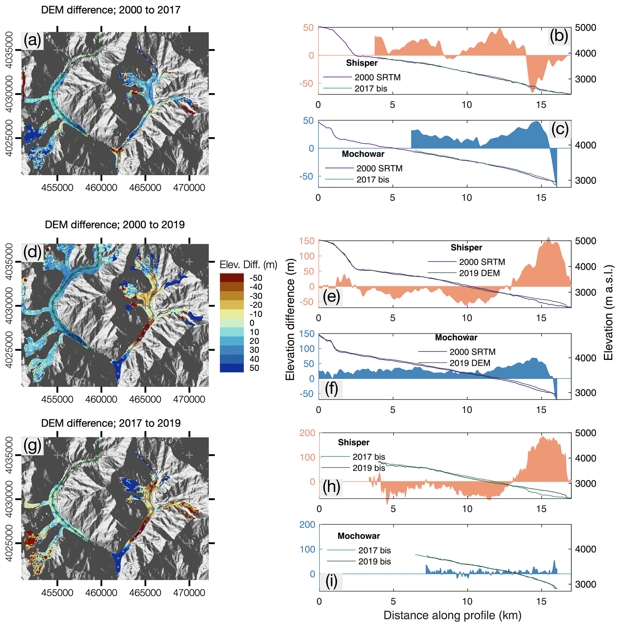
Figure 6Surface elevation changes at the Shisper and Mochowar glaciers between 2000, 2017, and 2019. The left column represents map views of the DEM differences and the right column displays the elevation differences and surface elevations along the profiles. The elevation difference is shaded above and below 0 to highlight mass gains (above) and mass loss (below). (a), (b), and (c) show the difference between the SRTM DEM of 2000 and the DEM created for 2017 with PlanetScope images (2017 bis); (d), (e), and (f) show the difference between the SRTM DEM of 2000 and the DEM extracted from GeoEye-1 and WorldView-2 stereo-pair imagery in 2019 (2019 DEM); and (g), (h), and (i) show the difference between the DEM created for 2017 (2017 bis) and 2019 (2019 bis) with PlanetScope images. Note that for the PlanetScope DEMs (2017 and 2019), the available imagery did not allow the creation of DEMs covering the entirety of the glaciers, hence the data gap in the upper reaches of either glacier. The creation of the DEMs is detailed in Aati and Avouac (2020). Perceptually uniform color maps are used in this figure to prevent visual distortion of the data (Crameri, 2018a, b).
5.3 Elevation changes at Shisper and Mochowar glaciers between 2000, 2017, and 2019
Both Shisper and Mochowar glaciers show increasing surface elevations between 2000 and 2017, with the exception of their terminus areas being constituted of ice left over by previous surges (Fig. 6a, b, and c). This increase in surface elevation can be likened to a positive mass balance, and is consistent with the Karakoram climatic anomaly (e.g., Gardelle et al., 2012; Kääb et al., 2015). The height increases on both glaciers (∼10 to 50 m over 17 years, Fig 6a, b, and c) are consistent with those measured by Gardelle et al. (2012, Fig. 3 therein), that are on the order of several tens of meters in about a decade. It is important to note, however, that the present study area is located on the western edge of the Karakoram region which is generally expected to undergo slightly negative mass balance budgets (Gardelle et al., 2012; Farinotti et al., 2020).
Because the latest surge of Shisper Glacier occurred between 2000 and 2005 (see Sect. S3), the SRTM DEM of 2000 is likely a representation of the surface of the glacier towards the end of its quiescence phase or beginning of the surge. Unfortunately the computed DEM, based on 2017 images, does not cover the icefall, but it shows a gain in elevation across the upper and main trunk. By contrast, the terminus shows a clear mass loss between 2000 and 2017 (Fig. 6b) where the stagnant ice from previous surges is expected. The area where the most elevation gain takes place is between kilometers 10 and 13, which corresponds to the lower part of the area where velocities are the fastest. The elevation gain in this area could also be the result of mass redistribution from the surge in the early 2000s that was smaller than the one described here.
Since 2000, almost the entire glacier surface has lowered as a result of the surge (Fig. 6d–i), with the exception of the terminus and lower section of the main trunk that acted as the receiving area during the surge (Fig. 6e and h). The area that undergoes the most lowering is part of the main trunk, between kilometers 8 and 13, located just upstream from where the observed velocities are the fastest (Fig. 6e and h). The surge emplaced up to 200 m of ice in the terminus region, with at least 100 m over the last 4 km of the glacier (Fig. 6e and h) which explains the dramatic advance and the fact that the terminus seems to keep on advancing even after the surge has terminated.
Similar to Shisper Glacier, the elevation change at Mochowar Glacier points to a positive mass balance since 2000, also consistent with the Karakoram anomaly (e.g., Gardelle et al., 2012; Kääb et al., 2015). The fact that both glaciers show similar patterns points to a climatic driver for surface elevation changes at both glaciers, rather than to an individual dynamic behavior (e.g., Roe and O'Neal, 2009). The drop in elevation seen in 0.5km of the profile is associated with the melting of stagnant ice left by a prior surge (see Sect. S3). It is worth noting that Mochowar and Shisper glaciers were connected until 2005. However, the last documented surge of Mochowar Glacier, prior to the current study, dates back to the 1970s (Bhambri et al., 2017).
The fact that the ice thickness increases by several tens of meters within ∼5 km of the terminus suggests that a slow surge actually took place, otherwise the thickening would be expected to be the largest at higher elevations. In addition, Mochowar Glacier shows significant seasonal signal with spring speed-up every year (Figs. S3.1 and S3.2). The data are noisy, but there seem to be a slight increase in velocities in 2018 (Fig. S3.1).
6.1 Spatiotemporal evolution of surge dynamics
The surge of Shisper Glacier shows a dramatic terminus advance. The terminus advanced by more than 1.7 km, emplacing up to 200 m of ice in the terminus region and more than 100 m over 4 km (Figs. 5c and 6). In comparison, the Haut-Glacier d'Arolla, Switzerland, was 180 m at its thickest, and 4 km long in the 1990s (Sharp et al., 1993). Interestingly, Shisper Glacier surged in early 2000s, but this older surge was much less pronounced since the terminus stopped ∼700 m up-valley from the surge presented here (see Sect. S3). We do not have enough information to discuss the differences between the two surges, but we suggest that the fast flow part of a surge cycle can vary over time. The possible differences between surge dynamics at a single glacier could suggest that surges follow a single mechanism with different manifestations, rather than different surging mechanisms linked to climatic regions (e.g., Murray et al., 2003; Quincey et al., 2015).
The velocity time series from Shisper Glacier suggests a clear correlation between surge dynamics and glacial hydrology. We find that the dynamic evolution of the glacier can be decomposed in the following patterns (Figs. 5 and 7): (1) a regular seasonal signal in both the spring and the fall until spring 2016, (2) a gradual increase in the magnitude of spring speed-ups in 2016 and 2017, (3) slow onset of the surge in November 2017, (4) Phase 1 of the main surge coinciding with the spring speed-up in 2018, (5) Phase 2 shows a slowdown in the surge with a short-term acceleration when a significant lake forms, (6) Phase 3 shows a significant increase in velocities that coincides with the spring speed-up in 2019, and (7) the surge terminates at the end of June 2019 in unison with the lake drainage. The consistent correlation between surge events and expected changes in glacial hydrology suggests that the surge represents a dynamic state where basal sliding is enhanced, but remains sensitive to hydraulic forcing.
Velocity fluctuations during surges appear to be commonplace when observations with a high-enough temporal resolution are available. The most striking example is the surge of Variegated Glacier in 1982–1983, where Kamb et al. (1985) recorded velocity fluctuations both at the seasonal scale, and within hours. Furthermore, they identified a clear link between glacier hydrology and velocity fluctuations during the surge, referring to these events as mini-surges. A two-phase surge with peak velocity associated with surface meltwater production was also identified for Kyagar Glacier in the Chinese Karakoram (Round et al., 2017). A gradual increase in surface velocities over several years leading up to the surge of Basin-3 in Austfonna, Svalbard, in the early 2010s, is reported in Dunse et al. (2015). Again, velocity peaks akin to spring speed-ups are present, even during the surge. However, the amplitude of the speed-ups does not appear to change significantly (see Fig. 2 in Dunse et al., 2015). Another example of seasonal velocity changes during a surge comes from Hagen Bræ, North Greenland (Solgaard et al., 2020), where both summer and winter speed-ups are also documented.
An interesting outcome of the current study is that using only L8 or S2 would have led to an incomplete picture of the dynamics of Shisper Glacier. The L8 data hold the information about the dynamics prior to the surge, and the S2 data show the intricacies of the surge onset and its different phases (Fig. S4.1). The main reason why we are able to identify the different dynamic events leading up to and during the surge is the quality and the spatiotemporal resolution of the velocity time series. Based on the differences between L8- and S2-derived datasets (Fig. S4.1; see also Fig. 3 in Bhambri et al., 2020), we suggest that the conundrums related to specific surge mechanisms and evolution in different regions of the world (e.g., Murray et al., 2003; Quincey et al., 2015) are in part due to observational limitations. It is also important to note that even in our dataset, such limitations exist as velocity changes can be significant at an hourly timescale (e.g., Kamb et al., 1985). The data quality furthermore allows us to identify the main trunk as the location of the surge initiation, and to suggest that, at Shisper Glacier, the dynamic response of the rest of the glacier is driven by the dynamics of the main trunk.
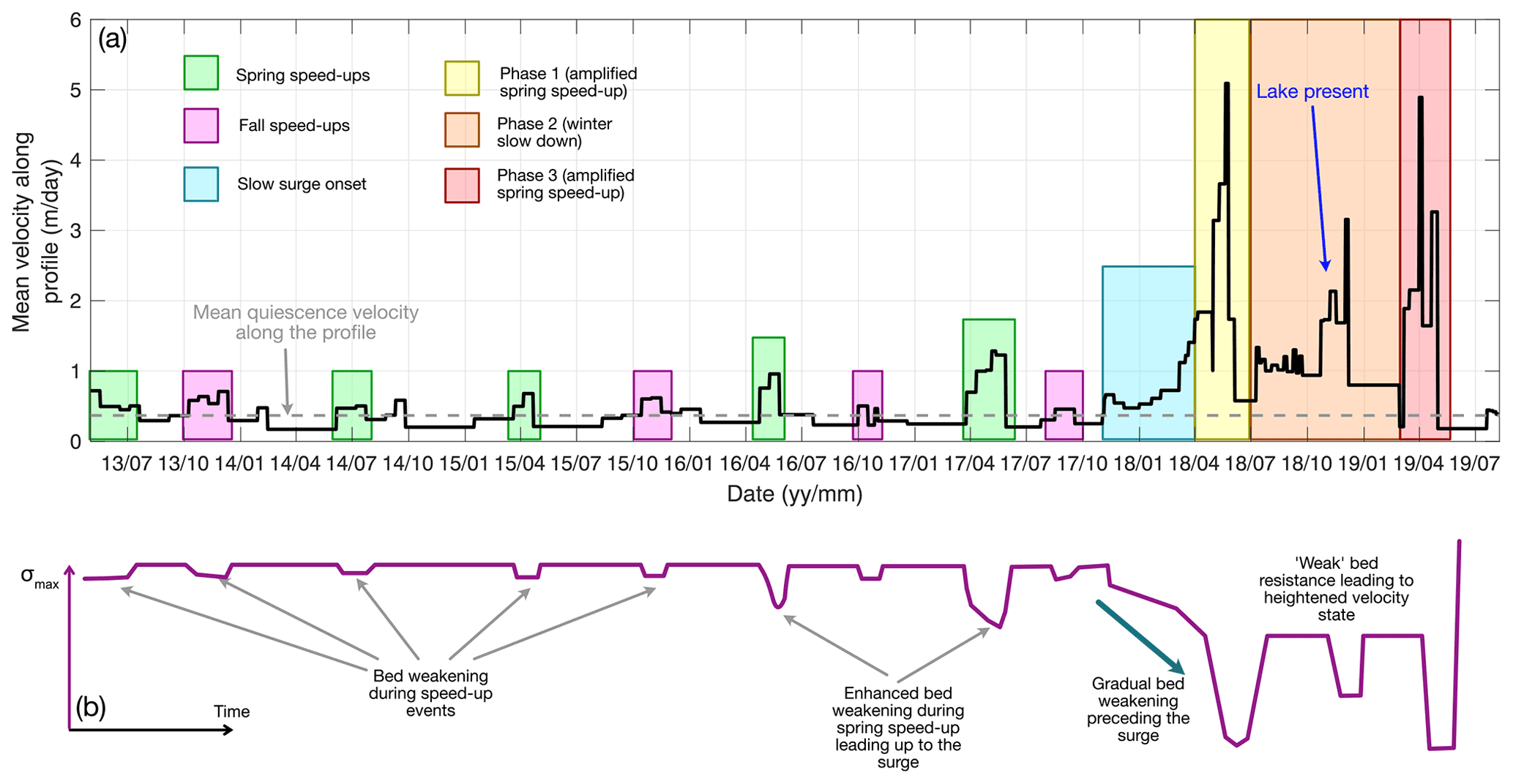
Figure 7(a) Spatial average of surface velocities along the profile of Shisper Glacier as a function of time and (b) conceptual representation of the maximum resistive stress σmax.
6.2 Interplay between lake drainage and surge termination
The surge termination coincides with the drainage of the glacier-dammed lake on 23 June 2019 (Fig. 5c; Pamir Times, 2019; Rashid et al., 2019). Cloud cover hampered our ability to utilize images collected around that time. Several coincident processes occur, which indicate that either the lake drainage affects the surge termination or vice versa. Surge termination is notoriously associated with a flood, whether it results from a glacier-dammed lake or subglacially stored water (e.g., Kamb et al., 1985; Round et al., 2017; Steiner et al., 2018; Zhan, 2019). During a surge, a distributed drainage system is necessary to maintain high water pressures. As a channelized drainage system forms, it is able to drain the water out of the glacier bed more efficiently, decreasing overall water pressures (e.g., Röthlisberger, 1972; Iken and Bindschadler, 1986; Björnsson, 1998; Mair et al., 2002; Werder and Funk, 2009), consequently terminating the surge (e.g., Kamb et al., 1985). In the case of Shisper Glacier, two scenarios are possible to explain this simultaneity: (1) the lake drainage initiated the onset of a channelized drainage under the whole glacier, or (2) the drainage of the water stored by the glacier during the surge opened waterways for the lake to drain. In the present study, we lack data to establish a causality between the two phenomena.
Here, and in other studies (Round et al., 2017; Steiner et al., 2018), lakes lay only about 1–3 km from the glacier terminus. The drainage of these lakes is synchronous with the termination of the surge. The lake drainage on 23 June 2019 only mildly affected Hassanabad Village, but severely damaged the Karakoram Highway (Pamir Times, 2019). The lake formed and drained again in 2020, this time, a month earlier, around 29 May, which could create a recurring hazard. Determining the causality between the lake drainage and surge-terminating flood would be important to determine the size of expected floods. If the volume of the stored water (Fig. S3.3) is added to that of the lake, the hazard could be much more important than if only the lake is considered.
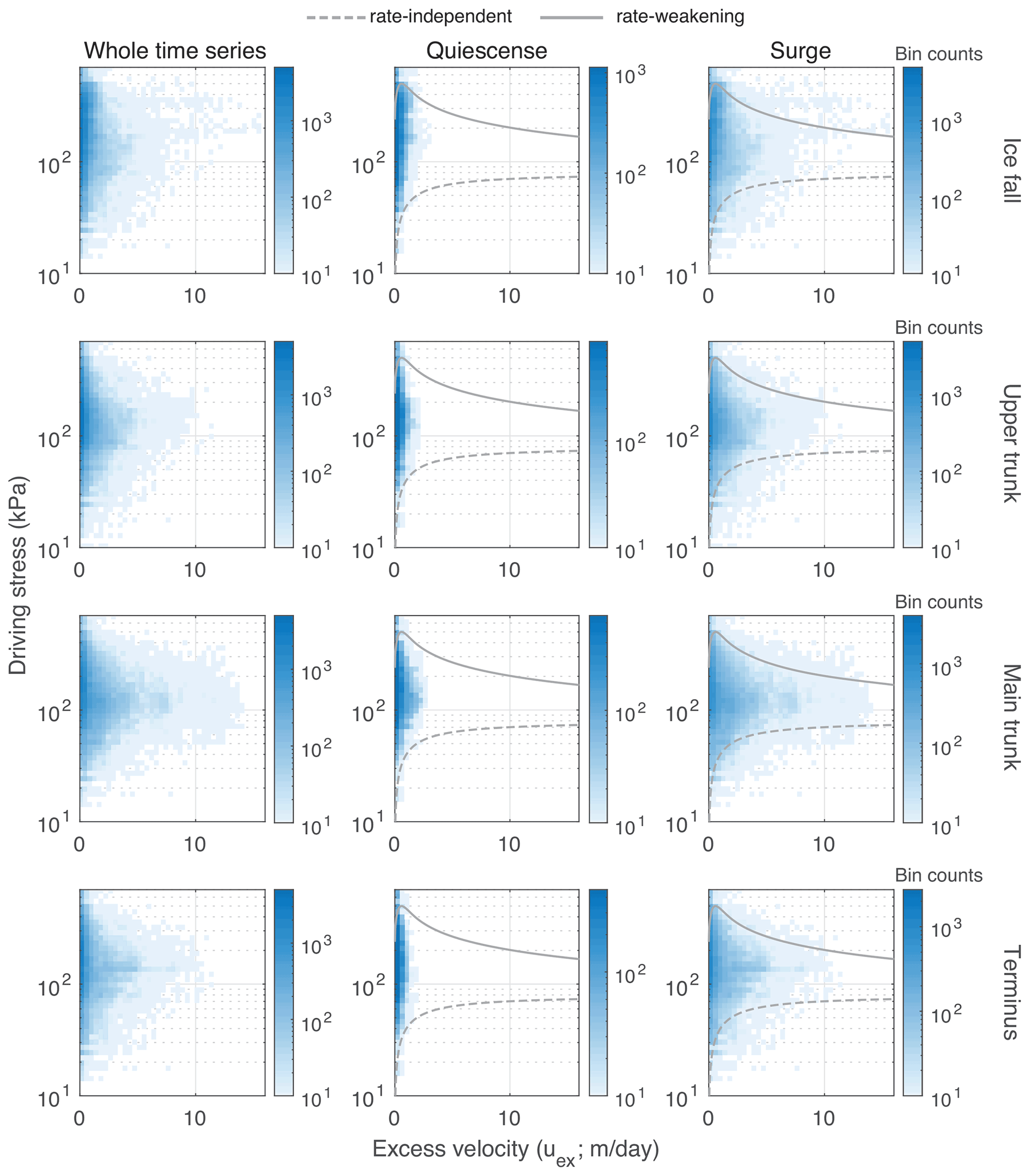
Figure 8Relationship between driving stress and excess velocities, used as a proxy for sliding velocities. The data on each axis are separated in 40 bins, and the plot color represents the number of data points within a bin. Rate-independent and rate-weakening behaviors are shown by the dashed and full lines, respectively. Note that the y axis is logarithmic and the x axis is linear, and the effect of axes scaling on data visualization is shown in Figs. S4.8 and S4.9.
6.3 Towards a unified glacier sliding relationship
We use the available data at Shisper Glacier to substantiate the behavior of the proposed generalized sliding relationship (Eq. 6) and to show the potential for future quantifications of sliding-law parameters. Because of major uncertainties in the bed-elevation data available and the lack of numerical modeling, we are not able to quantify resistive stresses. We can however use the available data to infer the presence of rate-independent and rate-weakening relationships between resistive stress and sliding speed during the surge. Changes in glacier velocity are the result of changes in the balance between driving and resistive stresses, thus if velocities increase significantly without a commensurate change in driving stress, the resistive stress must decrease.
We plot estimates of driving stresses and sliding velocities for Shisper Glacier to assess the behavior before and during the surge (Fig. 8). We use the DEMs available (Fig. 6) and the models of bed topography (Farinotti et al., 2019) to estimate the driving stress , where ρ is the ice density, g is the gravitational acceleration, hice is the ice thickness, and ∇Sice(x,y) is the ice surface gradient. To ensure that the velocity change used in the slip relationship is associated with sliding, and that deformation only accounts for a negligible fraction of the signal, we use the difference between surface velocities and the mean quiescence velocities (). We term this velocity difference the excess velocity (uex). The mean quiescence velocity () is calculated by time averaging the entire velocity field for each velocity map until the surge onset in November 2017. We expect this choice to lead to an overestimation of the mean quiescence velocity as it encompasses the enhanced speed-ups of 2015 and 2016. This underestimation of the sliding signal renders our assessment more conservative.
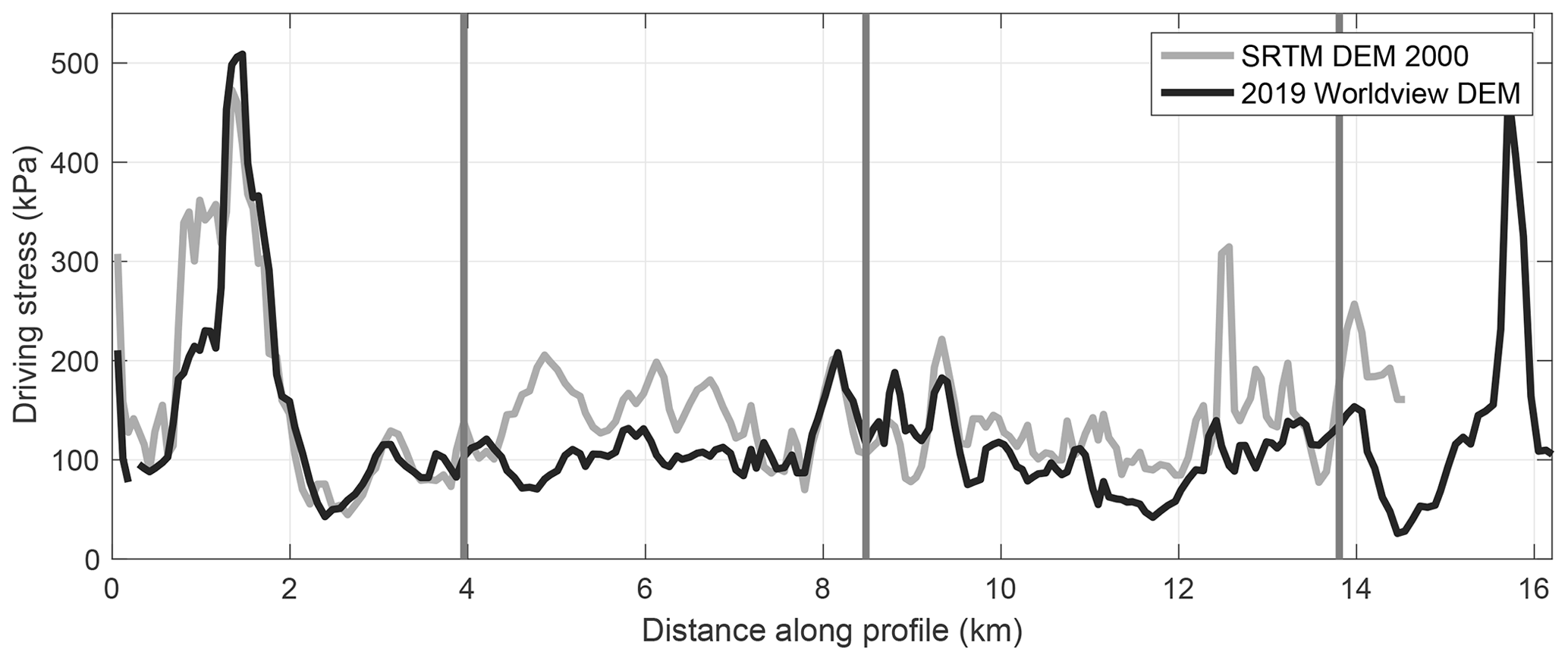
The main source of uncertainty to estimate driving stress is the ice geometry. We have no field data for bed elevation and lack data on the evolution of the ice surface during the surge. We choose to use the SRTM DEM of 2000 to calculate driving stresses from the beginning of the time series until the lake forms. Thereafter, we use the DEM of 2019 (Fig. 9). This is a somewhat arbitrary change based on the expected geometric evolution. It is important to note that using either DEM for the driving stress approximation does not alter the patterns significantly (Figs. S4.3 to S4.7). We divide the velocity dataset into four spatial zones, as delimited in Figs. 2 and 9, and two periods, i.e., the quiescence and the surge (see Fig. 8). We chose to lump the different phases of the surge together because we lack data on surface changes at a required temporal resolution during the event. The icefall and the front of the terminus show particularly high driving stresses because of surface slopes greater than 30∘ (Fig. 9).
We find that the relationship between driving stress and excess velocity can be comprised between two main behaviors: it either reaches an asymptote (dashed line) or decreases after a maximum value is reached (full line) for excess velocities (, Fig. 8). This observation stands across the different glacier regions. During the quiescence, where excess velocities remain smaller than , these trends are not apparent (with the exception of the main trunk where the speed-ups of 2015 and 2016 occurred) and hint at a commensurate evolution of driving stresses and excess velocities (Fig. S4.9). The icefall region shows particularly high driving stresses, and excess velocities are more scattered than for the rest of the dataset. The presence of clouds and snow over the topography at high elevations weakens image correlation, a likely source of the scatter, rendering the velocity data less reliable.
As driving stress reaches an asymptote or even decreases as excess velocity increases, resistive stress must also be bounded or decrease. This behavior is expected from the generalized sliding relationship (Eq. 6; Fig. 1). Previous studies show that for sliding velocities in excess of , the basal shear stress tends to be lower than the driving stress (Habermann et al., 2013; Hoffman and Price, 2014; Minchew et al., 2016; Vallot et al., 2017; Thøgersen et al., 2019), further solidifying our assessment. We thus suggest that the data presented substantiate the rate-independent or rate-weakening behavior as proposed in the generalized sliding relationship. The methods presented here, supported with a good bed map and an inversion for resistive stress, could lead to a quantification of the parameters of the sliding relationship.
6.4 Implications for glacier sliding
To date, attempts at validating a sliding relationship remain scarce and highlight the caveats of Weertman-type relationships (e.g., Bindschadler, 1983; Minchew et al., 2016; Vallot et al., 2017; Stearns and Van der Veen, 2018; Joughin et al., 2019). Minchew et al. (2016) use a combination of remote sensing and numerical modeling to show that sliding at the bed of Hofsjökull ice cap, Iceland, follows a plastic behavior. In a study combining numerical modeling and remote sensing to explore the dynamics of Kronebreen, a fast-flowing tidewater glacier in Svalbard, Vallot et al. (2017) find that the parameters of a sliding relationship should evolve in space and time to account for the behavior they observe. For fast ice flow at Pine Island Glacier, Antarctica, Joughin et al. (2019) show that a sliding relationship involving a Coulomb-type failure is necessary. Similarly, Stearns and Van der Veen (2018) show rate-independent shear stresses for several Greenlandic outlet glaciers. These studies have the following in common: they assume a deformable bed, and they are using mostly spatial changes, not time series.
Our dataset combined with the generalized sliding relationship allows us to bridge the gap between relatively slow glacier flow, with velocities comparable to Iceland during the quiescence, and fast ice flow, with velocities comparable to that of Greenlandic or Antarctic outlet glaciers. For example, Stearns and Van der Veen (2018), looking at 140 outlet glaciers in Greenland, find no relationship between velocity and basal shear stress, yet they find a correlation between velocities and their proxy for effective pressure. We suggest that these glaciers are undergoing a skin friction regime. The generalized sliding relationship further shows that the maximum bed resistance is mostly controlled by the effective pressure, and the relationship between velocities and basal shear stress in their dataset may exist via the effective pressure, although it is non trivial. Re-analyzing these datasets in light of the generalized sliding relationship could thus help to quantify the free parameters, σmax and ut, and gain valuable insight about the bed conditions of these outlet glaciers. Vallot et al. (2017) find that sliding parameters need to change in time and space to account for the evolution of sliding patterns. The span in driving stress versus excess velocity plot suggest that this is the case for Shisper Glacier too. Future quantifications should thus include a range of dynamic behaviors, even for a single glacier.
The results we present suggest that it is possible to test and quantify generalized sliding parameters globally. Our methods, completed with good bed-elevation data and extended with numerical modeling of the stress balance, would enable the inversion for the four key parameters in the generalized sliding relationship: ut, σmax, p, and q. These efforts are facilitated by the widespread availability of glacier surface velocities (e.g., Gardner et al., 2019). For such quantification to be efficient though, it is essential to focus on improving glacier bed-geometry measurements or estimations. Numerical modeling is also necessary to constrain the stress balance and isolate basal shear stresses (Habermann et al., 2013; Hoffman and Price, 2014; Minchew et al., 2016; Vallot et al., 2017; Thøgersen et al., 2019). In addition, the remote-sensing method we present is key to identifying subseasonal surface velocity fluctuations, shedding new light on global glacier dynamics.
6.5 Outlook on surge behavior
Traditionally, glacier surges are divided in two main categories, i.e., surges triggered by glacier hydrology and those triggered by a change in basal thermal regime (e.g., Meier and Post, 1969; Clarke et al., 1984; Jiskoot et al., 2000; Murray et al., 2000, 2003; Sevestre et al., 2015). The thermal trigger consists of an event that thaws a glacier bed that was previously frozen (e.g., Clarke et al., 1984; Murray et al., 2000). The hydraulic trigger refers to an increase in basal water pressure that reduces bed resistance (e.g., Kamb et al., 1985; Murray et al., 2003; Sevestre et al., 2015). Slow build-ups and terminations (e.g., Murray et al., 2003) are widely used criteria for identifying a thermal trigger (e.g., Quincey et al., 2015). By contrast, a hydraulic trigger is expected to produce more sudden velocity variations. While it remains a broadly recognized hypothesis (e.g., Farinotti et al., 2020), there is little direct evidence to support the thermal trigger of cyclic surges (Clarke et al., 1984; Frappé and Clarke, 2007; Sevestre et al., 2015).
Neither trigger mechanism provides an explanation as to why certain glaciers are surge-type and others are not. A global glacier analysis shows that surge-type glaciers are only found within certain climatic conditions (Sevestre et al., 2015). Benn et al. (2019) propose a theoretical model of glacier surge based on enthalpy and mass budgets that captures this climatic condition and can capture whether a glacier is stable (non-surge-type) or unstable (surge-type). In this model, enthalpy is gained by adding heat or water to the system. Since ice cannot be warmer than 0∘C, water content is necessary to track total heat content. Mass is gained by ice accumulation and lost by melt and flow. The enthalpy and mass budgets are intricately linked. For example, an increase in water content tends to yield faster ice flow, while an increase in heat production leads to more ice melt. The interplay between the two budgets is described in detail in Benn et al. (2019). An important element of this model is that basal shear heating can play an important role in the surge cycle.
At Shisper Glacier, the increase in spring speed-up amplitude, together with the pre- and post-surge differences in driving stress, are consistent with expected enthalpy and mass budgets. The gradual increase in spring speed-up amplitude suggests that the glacier is in an increasing energy state and increasingly sensitive to water pressure changes. This state of higher enthalpy appears to be happening at the same time as mass is gained.
Once the glacier is in an unstable equilibrium, any perturbation can start the surge. For Shisper Glacier, we infer that perturbation is caused by surface melt-dominated hydrology due to its periodic nature, rather than by a relatively steady meltwater production due to shear heating. Our data show a pre-surge history of both fall and spring speed-ups that appears to be linked to the glacier’s hydrology (Fig. 5), and thereafter the surge dynamics seem to be modulated by hydraulic events. Spring speed-ups are typically explained by an increase in water input overwhelming a mostly distributed subglacial drainage system (e.g., Müller and Iken, 1973; Iken and Truffer, 1997). On the other hand, the fall speed-up is typically explained by the closure of a channelized drainage system that leads to an overall increase in water pressure, although the input does not necessarily increase, and that mechanism has previously been proposed to explain surge initiation (e.g., Kamb, 1987; Abe and Furuya, 2015). The presence of fall speed-ups prior to the surge and its slow initiation showing a coinciding timing suggest that said fall speed-up is responsible for the surge onset. The first main phase of the surge is then triggered by the following spring speed-up.
Theories of subglacial water drainage suggest that subglacial waterways can adapt relatively rapidly to changing inputs (days to week), which would prevent a relatively slow increase in water input to trigger a sharp speed-up (Flowers, 2008; Werder et al., 2013). If we estimate the basal shear heating over the current dataset, we find that while it is non-negligible (Fig. S4.2), it produces significantly less melt than the expected surface melting if the mean daily temperature is above 2 ∘C. This is commensurate with the surface temperature at the time of the surge onset in the main trunk. We thus suggest that the basal shear heating likely plays an important role in sustaining relatively high water pressures and the high enthalpy state of the glacier leading up to, and during the surge, although it is unlikely to be a trigger due to its steady nature. In summary, at Shisper Glacier, hydraulic event triggers are necessary to drive each phase of the surge while the shear heating could be necessary to sustain surge velocities.
From Eqs. (4)–(6), we can further conclude that changes in N drive the different phases of the surge, rather than changes in driving stress or bed properties. Changes in bed properties, such as till strength, particle, or obstacle size, can be significant in space, but can be ignored over the timescale of a surge. Driving stresses change significantly during the surge (Fig. 9), with drops of up to 200 kPa between 2000 and 2019. Yet, such changes remain smaller than the expected fluctuations in N. Subdaily changes in N for Shisper Glacier are expected to be at least on the order of 100 kPa (∼10 m of water) as observed for small valley glaciers (e.g., Iken, 1981; Rada and Schoof, 2018), and up to 103 kPa as observed during the surge of Variegated Glacier (Kamb et al., 1985). For example, the significant mass wastage between the surge onset and Phase 3 is still not significant enough to prevent Phase 3 of the surge.
The generalized sliding relationship highlights the importance of effective pressure in controlling sliding throughout the surge. While we cannot readily express the generalized sliding relationship as a function of N, we can discuss its relative importance on σmax and ut. Both σmax and ut are controlled by a combination of N, bed properties and ice rheology at the bed (Eqs. 4 and 5).
Till strength for a given effective pressure shows little fluctuations (Iverson, 2010), and the particle size distribution is not expected to change significantly over the span of a surge. The re-arrangement of the orientation of large clasts could change till properties, yet that process has not been studied in detail. Over a rigid bed, variations in bed resistance arise from changes in bed geometry and ice flow-law coefficient (within parameter As). Considering that, for Shisper Glacier, the ice at the bed is at the pressure-melting point before the surge, it can be assumed that the parameter As is constant throughout the study period (Cuffey and Paterson, 2010). Furthermore, once the transition or skin friction regimes are reached, the effect of changes in driving stress become secondary, as long as it is greater than the basal shear stress (Fig. 1). We thus suggest that bed properties have a significant impact on the spatial distribution σmax and ut, and the temporal variations originate from changes in N almost uniquely.
The effective pressure, N, which depends on the ice thickness and basal fluid pressure, might be seen as a state variable that controls both the onset of unstable sliding, i.e., the transition and skin friction regimes, but also allows the recovery from fast sliding to occur (Fig. 7b). This means that both the surge initiation and termination can be hydraulically triggered. The idea that enhanced driving stresses lead to initiation, or that draining of glacier ice and resulting decrease in driving stresses can cause the surge to terminate, would require rates and amplitudes of driving stress changes that are unrealistic. Changes in glacier surface akin to those we observe over 2 years (DEMs of 2017 and 2019) would be necessary to bring the sliding regime into the transition regime or terminate the skin friction regime, under constant hydraulic conditions. Expecting these changes to occur over the time span of surge initiation or termination is unrealistic.
The generalized sliding relationship also offers a possible explanation for differences in surge dynamics, for example, whether the velocity increase is gradual or sudden. For bed conditions where the threshold velocity is relatively large and q=1, reaching skin friction will be gradual and the transition regime will span a large range of sliding velocities. This would result in a gradual increase in velocities towards the surge apex. Conversely, a relatively low-threshold velocity and large q would mean that the transition regime only spans a small range of velocities, and the skin friction regime is highly rate-weakening. The surge apex would be reached quickly, and surge velocities could remain particularly high until a significant water drainage event occurs.
We present a generalized sliding relationship for glaciers valid for both rigid and deformable beds, together with a remote-sensing workflow that allows us to substantiate this relationship from time series of optical images. The new remote-sensing workflow allows us to combine surface velocity time series, calculated from two different satellites systems (L8 and S2) and achieve a high spatiotemporal resolution. The combined dataset is then enhanced by post-processing steps that significantly improve data quality. We apply this remote-sensing workflow to the surge-type Shisper Glacier in Pakistan's Karakoram, and obtain a particularly detailed picture of the dynamic changes leading up to and during the recent surge. We find an increased amplitude of spring speed-ups in the few years leading up to the surge. Then the surge can be decomposed in a slow onset and three main phases. Importantly, these events appear to be linked to the hydraulic activity of the glacier. We thus suggest that the surge is a state of heightened velocity and sensitive to hydraulic changes.
Our estimation of driving stresses and sliding velocities show that sliding can increase independently of driving stress when sliding speeds are relatively large. This confirms the predictions from the generalized sliding relationship and the existence of transition and skin friction sliding regimes (i.e., rate-independent or rate-weakening) during the surge, while the quiescence appear to be characterized mostly by a form drag regime (i.e., rate-strengthening). The spring speed-up events likely represent incursions into the transition regime. The present study presents a proof of concept for a method to test glacier sliding relationships at a global scale, using mostly open-source data and software. We anticipate that reproducing such a study for a glacier with a good bed map and constraint on the ice surface evolution, combined with numerical modeling could yield a quantification of the sliding relationship parameters. Such studies will be essential to better understand glacier surges and the fast flow of tidewater glaciers in Patagonia, Alaska, Greenland, and Antarctica.
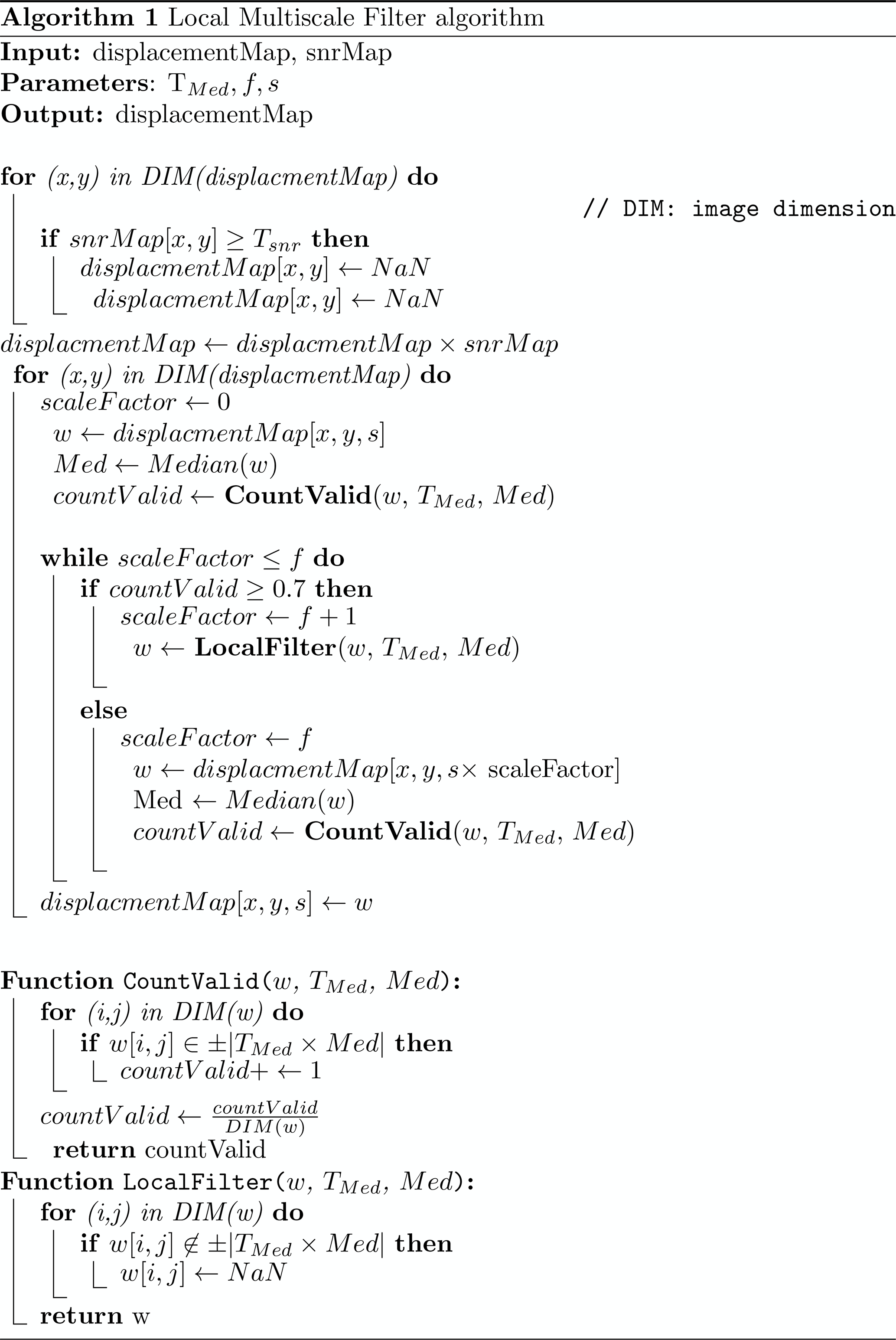
Algorithm for the post-processing of displacement maps.

The code for image correlation is available here http://www.tectonics.caltech.edu/slip_history/spot_coseis/download_software.html (Leprince et al., 2007). The dataset and code used for the analysis and data plotting is available here https://doi.org/10.5281/zenodo.4624397 (Beaud et al., 2021).
The supplement related to this article is available online at: https://doi.org/10.5194/tc-16-3123-2022-supplement.
JPA initiated the project and coordinated the work. JPA and SuA generated the funding. FB identified the study site. FB, SaA, ID, SuA, and JPA framed the research and formulated the goals. SaA developed the remote-sensing methodology and processed the data. FB helped to validate the velocity maps. SaA generated preliminary figures presenting the remote-sensing analysis and results. FB analyzed the remote-sensing data and created figures for the manuscript. FB laid out the generalized sliding relationship, created the conceptual figures and conducted the assessment of the sliding relationship. JPA and SuA contributed to the remote-sensing analysis and the interpretation of the results. FB led the writing of the manuscript. ID assisted with interpreting the processes surrounding the glacier surge and preparing the manuscript. FB, SaA, ID, SuA, and JPA edited the manuscript.
The contact author has declared that none of the authors has any competing interests.
Publisher's note: Copernicus Publications remains neutral with regard to jurisdictional claims in published maps and institutional affiliations.
The authors are very grateful for Shan Gremion's help in the early stages of the project. The authors would like to thank handling editor Nanna Bjørnholt Karlsson for their thoughtful input, as well as three anonymous reviewers and Douglas Benn for their constructive comments that helped to improve the manuscript. Flavien Beaud would like to thank Victor C. Tsai, Alex S. Gardner and many others for the joint Caltech–JPL group discussion on glacier sliding that greatly helped to formulate some of the ideas in this paper.
This research has been supported by the Caltech-JPL President's and Director's Fund program and the Resnick Sustainability Institute, and the Swiss National Science Fund Mobility Postdoc Fellowships (grant no. P2SKP2_171755; 2017–2019 and P400P2_191105; 2020–2021).
This paper was edited by Nanna Bjørnholt Karlsson and reviewed by Douglas Benn and three anonymous referees.
Aati, S. and Avouac, J.-P.: Optimization of optical image geometric modeling, application to topography extraction and topographic change measurements using PlanetScope and SkySat imagery, Remote Sensing, 12, 3418, https://doi.org/10.3390/rs12203418, 2020. a, b, c
Abe, T. and Furuya, M.: Winter speed-up of quiescent surge-type glaciers in Yukon, Canada, The Cryosphere, 9, 1183–1190, https://doi.org/10.5194/tc-9-1183-2015, 2015. a, b
Adhikari, S., Ivins, E., and Larour, E.: Mass transport waves amplified by intense Greenland melt and detected in solid Earth deformation, Geophys. Res. Lett., 44, 4965–4975, 2017. a
Armstrong, W. H., Anderson, R. S., and Fahnestock, M. A.: Spatial patterns of summer speedup on South central Alaska glaciers, Geophys. Res. Lett., 44, 9379–9388, 2017. a
Avouac, J.-P. and Leprince, S.: Geodetic imaging using optical systems, in: Reference Module in Earth Systems and Environmental Sciences, 387–424, Elsevier, https://doi.org/10.1016/B978-0-444-53802-4.00067-1, 2015. a
Beaud, F., Flowers, G. E., and Pimentel, S.: Seasonal-scale abrasion and quarrying patterns from a two-dimensional ice-flow model coupled to distributed and channelized subglacial drainage, Geomorphology, 219, 176–191, 2014. a
Beaud, F., Aati, S., Delaney, I., Adhikari, S., and Avouac, J.-P.: Dataset and code – Shisper glacier surge and sliding law (Version 1), Zenodo [data set], https://doi.org/10.5281/zenodo.4624397, 2021. a
Benn, D. I., Fowler, A., Hewitt, I. J., and Sevestre, H.: A general theory of glacier surges, J. Glaciol., 65, 701–716, 2019. a, b, c
Beyer, S., Kleiner, T., Aizinger, V., Rückamp, M., and Humbert, A.: A confined–unconfined aquifer model for subglacial hydrology and its application to the Northeast Greenland Ice Stream, The Cryosphere, 12, 3931–3947, https://doi.org/10.5194/tc-12-3931-2018, 2018. a
Bhambri, R., Hewitt, K., Kawishwar, P., and Pratap, B.: Surge-type and surge-modified glaciers in the Karakoram, Sci. Rep.-UK, 7, 15391, 2017. a, b
Bhambri, R., Watson, C., Hewitt, K., Haritashya, U., Kargel, J., Shahi, A., Chand, P., Kumar, A., Verma, A., and Govil, H.: The hazardous 2017–2019 surge and river damming by Shispare Glacier, Karakoram, Sci. Rep.-UK, 10, 1–14, https://doi.org/10.1038/s41598-020-61277-8, 2020. a, b, c, d, e, f
Bindschadler, R.: The importance of pressurized subglacial water in separation and sliding at the glacier bed, J. Glaciol., 29, 3–19, 1983. a, b, c
Björnsson, H.: Hydrological characteristics of the drainage system beneath a surging glacier, Nature, 395, 771–774, https://doi.org/10.1038/27384, 1998. a
Budd, W. F., Keage, P. L., and Blundy, N. A.: Empirical studies of ice sliding, J. Glaciol., 23, 157–170, 1979. a, b
Burgess, E. W., Forster, R. R., and Larsen, C. F.: Flow velocities of Alaskan glaciers, Nat. Commun., 4, 1–8, 2013. a
Catania, G., Stearns, L., Moon, T., Enderlin, E., and Jackson, R.: Future evolution of Greenland's marine-terminating outlet glaciers, J. Geophys. Res.-Earth, 125, e2018JF004873, https://doi.org/10.1029/2018JF004873 2020. a
Chundley, T. and Willis, I.: Glacier surges in the north-west West Kunlun Shan inferred from 1972 to 2017 Landsat imagery, J. Glaciol., 65, 1–12, https://doi.org/10.1017/jog.2018.94, 2019. a
Clarke, G.: Subglacial Processes, Annu. Rev. Earth Pl. Sc., 33, 247–276, https://doi.org/10.1146/annurev.earth.33.092203.122621, 2005. a
Clarke, G., Collins, S., and Thompson, D.: Flow, thermal structure, and subglacial conditions of a surge-type glacier, Can. J. Earth Sci., 21, 232–240, https://doi.org/10.1139/e84-024, 1984. a, b, c
Clarke, G. K., Schmok, J. P., Ommanney, C. S. L., and Collins, S. G.: Characteristics of surge-type glaciers, J. Geophys. Res.-Sol. Ea., 91, 7165–7180, 1986. a, b
Copland, L., Sylvestre, T., Bishop, M., Shroder, J., Seong, Y., Owen, L., Bush, A., and Kamp, U.: Expanded and recently increased glacier surging in the Karakoram, Arct. Antarct. Alp. Res., 43, 503–516, 2011. a, b
Crameri, F.: Scientific colour-maps, Zenodo, https://doi.org/10.5281/zenodo.1243862, 2018a. a, b, c
Crameri, F.: Geodynamic diagnostics, scientific visualisation and StagLab 3.0, Geosci. Model Dev., 11, 2541–2562, https://doi.org/10.5194/gmd-11-2541-2018, 2018b. a, b, c
Cuffey, K. M. and Paterson, W. S. B.: The Physics of Glaciers, Butterworth-Heinemann, Burlington, MA, USA, Forth edn., ISBN 9780123694614, 2010. a, b, c
Dehecq, A., Gourmelen, N., Gardner, A., Brun, F., Goldberg, D., Nienow, P., Berthier, E., Vincent, C., Wagnon, P., and Trouvé, E.: Twenty-first century glacier slowdown driven by mass loss in High Mountain Asia, Nat. Geosci., 12, 22, https://doi.org/10.1038/s41561-018-0271-9, 2019. a
Drusch, M., Bello, U. D., Carlier, S., Colin, O., Fernandez, V., Gascon, F., Hoersch, B., Isola, C., Laberinti, P., Martimort, P., Meygret, A., Spoto, F., Sy, O., Marchese, F., and Bargellini, P.: Sentinel-2: ESA's Optical High-Resolution Mission for GMES Operational Services, Remote Sens. Environ., 120, 25–36, https://doi.org/10.1016/j.rse.2011.11.026, 2012. a
Dunse, T., Schellenberger, T., Hagen, J. O., Kääb, A., Schuler, T. V., and Reijmer, C. H.: Glacier-surge mechanisms promoted by a hydro-thermodynamic feedback to summer melt, The Cryosphere, 9, 197–215, https://doi.org/10.5194/tc-9-197-2015, 2015. a, b, c
ESA: European Space Agency, Copernicus Open Access Hub, https://scihub.copernicus.eu/, last access: 15 August 2019. a
Farinotti, D., Brinkerhoff, D. J., Clarke, G. K. C., Fürst, J. J., Frey, H., Gantayat, P., Gillet-Chaulet, F., Girard, C., Huss, M., Leclercq, P. W., Linsbauer, A., Machguth, H., Martin, C., Maussion, F., Morlighem, M., Mosbeux, C., Pandit, A., Portmann, A., Rabatel, A., Ramsankaran, R., Reerink, T. J., Sanchez, O., Stentoft, P. A., Singh Kumari, S., van Pelt, W. J. J., Anderson, B., Benham, T., Binder, D., Dowdeswell, J. A., Fischer, A., Helfricht, K., Kutuzov, S., Lavrentiev, I., McNabb, R., Gudmundsson, G. H., Li, H., and Andreassen, L. M.: How accurate are estimates of glacier ice thickness? Results from ITMIX, the Ice Thickness Models Intercomparison eXperiment, The Cryosphere, 11, 949–970, https://doi.org/10.5194/tc-11-949-2017, 2017. a
Farinotti, D., Huss, M., Fürst, J. J., Landmann, J., Machguth, H., Maussion, F., and Pandit, A.: A consensus estimate for the ice thickness distribution of all glaciers on Earth, Nat. Geosci., 12, 168, https://doi.org/10.1038/s41561-019-0300-3, 2019. a, b
Farinotti, D., Immerzeel, W. W., de Kok, R. J., Quincey, D. J., and Dehecq, A.: Manifestations and mechanisms of the Karakoram glacier Anomaly, Nat. Geosci., 13, 8–16, 2020. a, b, c
Flowers, G. E.: Subglacial modulation of the hydrograph from glacierized basins, Hydrol. Process., 22, 3903–3918, https://doi.org/10.1002/hyp.7095, 2008. a
Flowers, G. E.: Modelling water flow under glaciers and ice sheets, P. Roy. Soc. A, 471, 1–41, https://doi.org/10.1098/rspa.2014.0907, 2015. a
Frappé, T.-P. and Clarke, G. K. C.: Slow surge of Trapridge Glacier, Yukon Territory, Canada, J. Geophys. Res.-Earth, 112, F03S32, https://doi.org/10.1029/2006JF000607, 2007. a
Gagliardini, O., Cohen, D., Råback, P., and Zwinger, T.: Finite-element modeling of subglacial cavities and related friction law, J. Geophys. Res.-Earth, 112, F02027, https://doi.org/10.1029/2006JF000576, 2007. a, b, c, d, e, f
Gardelle, J., Berthier, E., and Arnaud, Y.: Slight mass gain of Karakoram glaciers in the early twenty-first century, Nat. Geosci., 5, 322–325, 2012. a, b, c, d, e
Gardner, A., Fahnestock, M., and Scambos, T.: ITS_LIVE regional glacier and ice sheet surface velocities, National Snow and Ice Data Center (NSIDC), https://doi.org/10.5067/6II6VW8LLWJ7, 2019. a, b, c
Gascon, F., Bouzinac, C., Thépaut, O., Jung, M., Francesconi, B., Louis, J., Lonjou, V., Lafrance, B., Massera, S., Gaudel-Vacaresse, A., Languille, F., Alhammoud, B., Viallefont, F., Pflug, B., Bieniarz, J., Clerc, S., Pessiot, L., Trémas, T.and Cadau, E., De Bonis, R., Isola, C., Martimort, P., and Fernandez, V.: Copernicus Sentinel-2A Calibration and Products Validation Status, Remote Sensing, 9, 584, https://doi.org/10.3390/rs9060584, 2017. a
Gelaro, R., McCarty, W., Suárez, M. J., Todling, R., Molod, A., Takacs, L., Randles, C. A., Darmenov, A., Bosilovich, M. G., Reichle, R., Wargan, K., Coy, L., Cullather, R., Draper, C., Akella, S., Buchard, V., Conaty, A., da Silva, A. M., Gu, W., Kim, G., Koster, R., Lucchesi, R., Merkova, D., Nielsen, J. E., Partyka, G., Pawson, S., Putman, W., Rienecker, M., Schubert, S. D., Sienkiewicz, M., and Zhao, B.: The modern-era retrospective analysis for research and applications, version 2 (MERRA-2), J. Climate, 30, 5419–5454, 2017. a
Habermann, M., Truffer, M., and Maxwell, D.: Changing basal conditions during the speed-up of Jakobshavn Isbræ, Greenland, The Cryosphere, 7, 1679–1692, https://doi.org/10.5194/tc-7-1679-2013, 2013. a, b
Heid, T. and Kääb, A.: Evaluation of existing image matching methods for deriving glacier surface displacements globally from optical satellite imagery, Remote Sens. Environ., 118, 339–355, https://doi.org/10.1016/J.RSE.2011.11.024, 2012. a, b
Hewitt, K.: Glacier surges in the Karakoram Himalaya (central Asia), Can. J. Earth Sci., 6, 1009–1018, 1969. a, b
Hewitt, K.: The Karakoram anomaly? Glacier expansion and the “Elevation Effect”, Karakoram Himalaya, Mt. Res. Dev., 25, 332–341, 2005. a
Hewitt, K. and Liu, J.: Ice-dammed lakes and outburst floods, Karakoram Himalaya: historical perspectives on emerging threats, Phys. Geogr., 31, 528–551, https://doi.org/10.2747/0272-3646.31.6.528, 2010. a
Hoffman, M. and Price, S.: Feedbacks between coupled subglacial hydrology and glacier dynamics, J. Geophys. Res., 119, 414–436, https://doi.org/10.1002/2013JF002943, 2014. a, b
Iken, A.: The effect of the subglacial water pressure on the sliding velocity of a glacier in an idealized numerical model, J. Glaciol., 27, 407–421, 1981. a, b, c, d, e
Iken, A. and Bindschadler, R. A.: Combined measurements of subglacial water pressure and surface velocity of Findelengletscher, Switzerland: conclusions about drainage system and sliding mechanism, J. Glaciol., 32, 101–119, 1986. a, b
Iken, A. and Truffer, M.: The relationship between subglacial water pressure and velocity of Findelengletscher, Switzerland, during its advance and retreat, J. Glaciol., 43, 328–338, https://doi.org/10.3189/S0022143000003282, 1997. a, b
Iverson, N. and Zoet, L.: Experiments on the dynamics and sedimentary products of glacier slip, Geomorphology, 244, 121–134, https://doi.org/10.1016/j.geomorph.2015.03.027, 2015. a
Iverson, N. R.: Shear resistance and continuity of subglacial till: hydrology rules, J. Glaciol., 56, 1104–1114, 2010. a, b, c, d
Iverson, N. R. and Iverson, R. M.: Distributed shear of subglacial till due to Coulomb slip, J. Glaciol., 47, 481–488, 2001. a, b, c, d, e, f
Jay-Allemand, M., Gillet-Chaulet, F., Gagliardini, O., and Nodet, M.: Investigating changes in basal conditions of Variegated Glacier prior to and during its 1982–1983 surge, The Cryosphere, 5, 659–672, https://doi.org/10.5194/tc-5-659-2011, 2011. a
Jiskoot, H.: Glacier surging, Encyclopedia of Snow, Ice and Glaciers, 415–428, 2011. a
Jiskoot, H., Murray, T., and Boyle, P.: Controls on the distribution of surge-type glaciers in Svalbard, J. Glaciol., 46, 412–422, 2000. a, b, c
Joughin, I., Smith, B., and Schoof, C.: Regularized Coulomb Friction Laws for Ice Sheet Sliding: Application to Pine Island Glacier, Antarctica, Geophys. Res. Lett., 46, 4764–4771, https://doi.org/10.1029/2019GL082526, 2019. a, b, c, d
Kääb, A., Treichler, D., Nuth, C., and Berthier, E.: Brief Communication: Contending estimates of 2003–2008 glacier mass balance over the Pamir–Karakoram–Himalaya, The Cryosphere, 9, 557–564, https://doi.org/10.5194/tc-9-557-2015, 2015. a, b, c
Kääb, A., Winsvold, S., Altena, B., N., C., Nagler, T., and Wuite, J.: Glacier Remote Sensing Using Sentinel-2. Part I: Radiometric and Geometric Performance, and Application to Ice Velocity, Remote Sensing, 8, 598, https://doi.org/10.3390/rs8070598, 2016. a
Kamb, B.: Glacier surge mechanism based on linked cavity configuration of the basal water conduit system, J. Geophys. Res.-Sol. Ea., 92, 9083–9100, 1987. a
Kamb, B., Raymond, C., Harrison, W., Engelhardt, H., Echelmeyer, K., Humphrey, N., Brugman, M., and Pfeffer, T.: Glacier surge mechanism: 1982–1983 surge of Variegated Glacier, Alaska, Science, 227, 469–479, 1985. a, b, c, d, e, f, g, h, i
Karim, D., Karim, I., Anwar, W., Uddin, K., Ali, A., and Gurung, D.: Glacier hazard associated with surging glaciers–story of the Shishper Glacier from Hunza, Pakistan, in: Debris Flows: Disaster, Risk, Forecast, Protection, Proceedings of the 6th conference, Dushanbe-Khorog, Tajikistan, 20–26 September 2020, edited by: Chernomorets, S. S. and Viskhadzhieva, K. S., 1, 234–245, Dushanbe: “Promotion” LLC, 2020. a
King, M. D., Howat, I. M., Jeong, S., Noh, M. J., Wouters, B., Noël, B., and van den Broeke, M. R.: Seasonal to decadal variability in ice discharge from the Greenland Ice Sheet, The Cryosphere, 12, 3813–3825, https://doi.org/10.5194/tc-12-3813-2018, 2018. a
Leprince, S., Barbot, S., Ayoub, F., and Avouac, J.-P.: Automatic and precise orthorectification, coregistration, and subpixel correlation of satellite images, application to ground deformation measurements, IEEE T. Geosci. Remote, 45, 1529–1558, https://doi.org/10.1109/TGRS.2006.888937, 2007 (data available at: http://www.tectonics.caltech.edu/slip_history/spot_coseis/download_software.html, last access: 15 February 2020). a, b, c, d
Lliboutry, L.: General theory of subglacial cavitation and sliding of temperate glaciers, J. Glaciol., 7, 21–58, 1968. a, b, c, d
MacAyeal, D. R.: Revisiting Weertman's tombstone bed, Ann. Glaciol., 60, 21–29, 2019. a
Mair, D., Nienow, P., Sharp, M., Wohlleben, T., and Willis, I.: Influence of subglacial drainage system evolution on glacier surface motion: Haut Glacier d'Arolla, Switzerland, J. Geophys. Res., 107, 10–1029, 2002. a
Mayer, C., Fowler, A., Lambrecht, A., and Scharrer, K.: A surge of North Gasherbrum Glacier, Karakoram, China, J. Glaciol., 57, 904–916, https://doi.org/10.3189/002214311798043834, 2011. a
Meier, M. and Post, A.: What are glacier surges?, Can. J. Earth Sci., 6, 807–817, 1969. a, b, c, d
Minchew, B. and Joughin, I.: Toward a universal glacier slip law, Science, 368, 29–30, 2020. a, b
Minchew, B., Simons, M., Björnsson, H., Pálsson, F., Morlighem, M., Seroussi, H., Larour, E., and Hensley, S.: Plastic bed beneath Hofsjökull Ice Cap, central Iceland, and the sensitivity of ice flow to surface meltwater flux, J. Glaciol., 62, 147–158, 2016. a, b, c, d, e, f, g
Moon, T., Joughin, I., Smith, B., Van Den Broeke, M. R., Van De Berg, W. J., Noël, B., and Usher, M.: Distinct patterns of seasonal Greenland glacier velocity, Geophys. Res. Lett., 41, 7209–7216, 2014. a
Mouginot, J., Rignot, E., Bjørk, A. A., Van den Broeke, M., Millan, R., Morlighem, M., Noël, B., Scheuchl, B., and Wood, M.: Forty-six years of Greenland Ice Sheet mass balance from 1972 to 2018, P. Natl. Acad. Sci. USA, 116, 9239–9244, 2019. a, b
Müller, F. and Iken, A.: Velocity fluctuations and water regime of Arctic valley glaciers, International Association of Scientific Hydrology Publication, 95, 165–182, 1973. a
Murray, T., Stuart, G., Miller, P., Woodward, J., Smith, A., Porter, P., and Jiskoot, H.: Glacier surge propagation by thermal evolution at the bed, J. Geophys. Res.-Sol. Ea., 105, 13491–13507, https://doi.org/10.1029/2000JB900066, 2000. a, b
Murray, T., Strozzi, T., Luckman, A., Jiskoot, H., and Christakos, P.: Is there a single surge mechanism? Contrasts in dynamics between glacier surges in Svalbard and other regions, J. Geophys. Res.-Sol. Ea., 108, 2237, https://doi.org/10.1029/2002JB001906, 2003. a, b, c, d, e
Pamir Times: Flood from advancing Shisper glacier damages a portion of KKH in Hasanabad, Hunza, https://pamirtimes.net/2019/06/23/flood-from-advancing-shisper-glacier-damages-a-portion-of-kkh-in-hasanabad-hunza/ (last access: 15 February 2020), 2019. a, b, c
Pattyn, F. and Morlighem, M.: The uncertain future of the Antarctic Ice Sheet, Science, 367, 1331–1335, 2020. a
Paul, F.: A 60-year chronology of glacier surges in the central Karakoram from the analysis of satellite image time-series, Geomorphology, 352, 106993, https://doi.org/10.1016/j.geomorph.2019.106993, 2020. a
Pfeffer, W., Arendt, A., Bliss, A., Bolch, T., Cogley, J., Gardner, A., Hagen, J.-O., Hock, R., Kaser, G., Kienholz, C., Miles, E. S., Moholdt, G., Mölg, N., Paul, F., Radić, V., Rastner, P., Raup, B. H., Rich, J., Sharp, M. J., and The Randolph Consortium: The Randolph Glacier Inventory: a globally complete inventory of glaciers, J. Glaciol., 60, 537–552, https://doi.org/10.3189/2014JoG13J176, 2014. a
Pimentel, S. and Flowers, G. E.: A numerical study of hydrologically driven glacier dynamics and subglacial flooding, P. Roy. Soc. A, 467, 537–558, https://doi.org/10.1098/rspa.2010.0211, 2010. a, b, c
Post, A.: Distribution of surging glaciers in western North America, J. Glaciol., 8, 229–240, 1969. a
Quincey, D., Braun, M., Glasser, N., Bishop, M., Hewitt, K., and Luckman, A.: Karakoram glacier surge dynamics, Geophys. Res. Lett., 38, L18504, https://doi.org/10.1029/2011GL049004, 2011. a
Quincey, D., Glasser, N., Cook, S., and Luckman, A.: Heterogeneity in Karakoram glacier surges, J. Geophys. Res.-Earth, 120, 1288–1300, https://doi.org/10.1002/2015JF003515, 2015. a, b, c, d
Rada, C. and Schoof, C.: Channelized, distributed, and disconnected: subglacial drainage under a valley glacier in the Yukon, The Cryosphere, 12, 2609–2636, https://doi.org/10.5194/tc-12-2609-2018, 2018. a
Rashid, I., Majeed, U., Jan, A., and Glasser, N.: The January 2018 to September 2019 surge of Shisper Glacier, Pakistan, detected from remote sensing observations, Geomorphology, 106957, https://doi.org/10.1016/j.geomorph.2019.106957, 2019. a, b, c, d, e
Roe, G. H. and O'Neal, M. A.: The response of glaciers to intrinsic climate variability: observations and models of late-Holocene variations in the Pacific Northwest, J. Glaciol., 55, 839–854, 2009. a
Rosu, A.-M., Pierrot-Deseilligny, M., Delorme, A., Binet, R., and Klinger, Y.: Measurement of ground displacement from optical satellite image correlation using the free open-source software MicMac, ISPRS J. Photogramm., 100, 48–59, https://doi.org/10.1016/J.ISPRSJPRS.2014.03.002, 2015. a, b
Röthlisberger, H.: Water pressure in intra- and subglacial channels, J. Glaciol., 11, 177–203, 1972. a
Round, V., Leinss, S., Huss, M., Haemmig, C., and Hajnsek, I.: Surge dynamics and lake outbursts of Kyagar Glacier, Karakoram, The Cryosphere, 11, 723–739, https://doi.org/10.5194/tc-11-723-2017, 2017. a, b, c, d
Roy, D., Wulder, M., Loveland, T., C.E., W., Allen, R., Anderson, M. C., Helder, D., Irons, J., Johnson, D., Kennedy, R., Scambos, T., Schaaf, C., Schott, J., Sheng, Y., Vermote, E., Belward, A., Bindschadler, R., Cohen, W., Gao, F., Hipple, J., Hostert, P., Huntington, J., Justice, C., Kilic, A., Kovalskyy, V., Lee, Z., Lymburner, L., Masek, J., McCorkel, J., Shuai, Y., Trezza, R., Vogelmann, J., Wynne, R., and Zhu, Z.: Landsat-8: Science and product vision for terrestrial global change research, Remote Sens. Environ., 145, 154–172, https://doi.org/10.1016/j.rse.2014.02.001, 2014. a
Rupnik, E., Daakir, M., and Pierrot-Deseilligny, M.: MicMac – a free, open-source solution for photogrammetry, Open Geospatial Data, Software and Standards, 2, 14, https://doi.org/10.1186/s40965-017-0027-2, 2017. a
Schoof, C.: The effect of cavitation on glacier sliding, P. Roy. Soc. Lond. A, 461, 609–627, 2005. a, b, c, d, e, f, g
Sevestre, H. and Benn, D.: Climatic and geometric controls on the global distribution of surge-type glaciers: implications for a unifying model of surging, J. Glaciol., 61, 646–662, https://doi.org/10.3189/2015JoG14J136, 2015. a, b, c
Sevestre, H., Benn, D. I., Hulton, N. R., and Bælum, K.: Thermal structure of Svalbard glaciers and implications for thermal switch models of glacier surging, J. Geophys. Res.-Earth, 120, 2220–2236, 2015. a, b, c, d
Shah, A., Ali, K., Nizami, S., Jan, I., Hussain, I., and Begum, F.: Risk assessment of Shishper Glacier, Hassanabad Hunza, North Pakistan, Journal of Himalayan Earth Sciences Volume, 52, 1–11, 2019. a
Sharp, M., Richards, K., Willis, I., Arnold, N., Nienow, P., Lawson, W., and Tison, J.-L.: Geometry, bed topography and drainage system structure of the Haut Glacier d'Arolla, Switzerland, Earth Surf. Proc. Land., 18, 557–571, 1993. a
Solgaard, A., Simonsen, S., Grinsted, A., Mottram, R., Karlsson, N., Hansen, K., Kusk, A., and Sørensen, L.: Hagen Bræ: A surging glacier in North Greenland–35 years of observations, Geophys. Res. Lett., 47, 2019GL085802, https://doi.org/10.1029/2019GL085802, 2020. a
Stearns, L. and Van der Veen, C.: Friction at the bed does not control fast glacier flow, Science, 361, 273–277, 2018. a, b, c, d, e
Steiner, J. F., Kraaijenbrink, P. D. A., Jiduc, S. G., and Immerzeel, W. W.: Brief communication: The Khurdopin glacier surge revisited – extreme flow velocities and formation of a dammed lake in 2017, The Cryosphere, 12, 95–101, https://doi.org/10.5194/tc-12-95-2018, 2018. a, b, c
NASA/METI/AIST/Japan Spacesystems and U.S./Japan ASTER Science Team: ASTER Global Digital Elevation Model V003. 2018, NASA EOSDIS Land Processes DAAC, https://doi.org/10.5067/ASTER/ASTGTM.003, 2018. a
Thøgersen, K., Gilbert, A., Schuler, T. V., and Malthe-Sørenssen, A.: Rate-and-state friction explains glacier surge propagation, Nat. Commun., 10, 1–8, 2019. a, b, c, d
Tsai, V. C., Stewart, A. L., and Thompson, A. F.: Marine ice-sheet profiles and stability under Coulomb basal conditions, J. Glaciol., 61, 205–215, 2015. a, b
Tulaczyk, S., Kamb, W. B., and Engelhardt, H. F.: Basal mechanics of ice stream B, West Antarctica: 1. Till mechanics, J. Geophys. Res.-Sol. Ea., 105, 463–481, 2000. a, b, c, d, e, f
U.S. Geological Survey: Digital Elevation – Shuttle Radar Topography Mission (SRTM) 1 Arc-Second Global, U. S. Geological Survey, Earth Resources Observation and Science (EROS) Center, https://doi.org/10.5066/F7PR7TFT, 2014. a, b
U.S. Geological Survey: Landsat 8 images, United States Geological Survey, https://earthexplorer.usgs.gov/, last access: 15 August 2019. a
Vallot, D., Pettersson, R., Luckman, A., Benn, D. I., Zwinger, T., Van Pelt, W. J., Kohler, J., Schäfer, M., Claremar, B., and Hulton, N. R.: Basal dynamics of Kronebreen, a fast-flowing tidewater glacier in Svalbard: non-local spatio-temporal response to water input, J. Glaciol., 63, 1012–1024, 2017. a, b, c, d, e
van de Wal, R. S. W., Smeets, C. J. P. P., Boot, W., Stoffelen, M., van Kampen, R., Doyle, S. H., Wilhelms, F., van den Broeke, M. R., Reijmer, C. H., Oerlemans, J., and Hubbard, A.: Self-regulation of ice flow varies across the ablation area in south-west Greenland, The Cryosphere, 9, 603–611, https://doi.org/10.5194/tc-9-603-2015, 2015. a
Weertman, J.: On the sliding of glaciers, J. Glaciol., 3, 33–38, 1957. a
Weertman, J.: General theory of water flow at the base of a glacier or ice sheet, Rev. Geophys., 10, 287–333, 1972. a, b
Werder, M. A. and Funk, M.: Dye tracing a jökulhlaup: II. Testing a jökulhlaup model against flow speeds inferred from measurements, J. Glaciol., 55, 899–908, 2009. a
Werder, M. A., Hewitt, I. J., Schoof, C. G., and Flowers, G. E.: Modeling channelized and distributed subglacial drainage in two dimensions, J. Geophys. Res.-Earth, 118, 2140–2158, 2013. a
Zhan, Z.: Seismic Noise Interferometry Reveals Transverse Drainage Configuration Beneath the Surging Bering Glacier, Geophys. Res. Lett., 46, 4747–4756, https://doi.org/10.1029/2019GL082411, 2019. a
Zoet, L. K. and Iverson, N. R.: Experimental determination of a double-valued drag relationship for glacier sliding, J. Glaciol., 61, 1–7, 2015. a, b, c, d
Zoet, L. K. and Iverson, N. R.: A slip law for glaciers on deformable beds, Science, 368, 76–78, 2020. a, b, c, d, e
- Abstract
- Introduction
- Generalized sliding relationship
- Study area and dataset
- Data processing
- Results
- Discussion
- Conclusions
- Appendix A: Algorithm
- Appendix B: Summary of symbols.
- Code and data availability
- Author contributions
- Competing interests
- Disclaimer
- Acknowledgements
- Financial support
- Review statement
- References
- Supplement