Towards accurate quantification of ice content in permafrost of the Central Andes – Part 2: An upscaling strategy of geophysical measurements to the catchment scale at two study sites

With ongoing climate change, there is a pressing need to better understand how much water is stored as ground ice in areas with extensive permafrost occurrence, as well as how the regional water balance may alter in response to the potential generation of meltwater from permafrost degradation. However, field-based data on permafrost in remote and mountainous areas such as the South American Andes are scarce. Most current ground ice estimates are based on broadly generalized assumptions such as volume–area scaling and mean ground ice content estimates of rock glaciers. In addition, ground ice contents in permafrost areas outside of rock glaciers are usually not considered, resulting in a significant uncertainty regarding the volume of ground ice in the Andes and its hydrological role. In Part 1 of this contribution, Hilbich et al. (2022a) present an extensive geophysical data set based on electrical resistivity tomography and refraction seismic tomography surveys to detect and quantify ground ice of different landforms and surface types in several study regions in the semi-arid Andes of Chile and Argentina with the aim to contribute to the reduction of this data scarcity. In Part 2 we focus on the development of a strategy for the upscaling of geophysics-based ground ice quantification to an entire catchment to estimate the total ground ice volume (and its approximate water equivalent) in the study areas. In addition to the geophysical data, the upscaling approach is based on a permafrost distribution model and classifications of surface and landform types. In this paper, we introduce our upscaling strategy, and we demonstrate that the estimation of large-scale ground ice volumes can be improved by including (i) non-rock-glacier permafrost occurrences and (ii) field evidence through a large number of geophysical surveys and ground truthing information. The results of our study indicate that (i) conventional ground ice estimates for rock-glacier-dominated catchments without in situ data may significantly overestimate ground ice contents and (ii) substantial volumes of ground ice may also be present in catchments where rock glaciers are lacking.

1 Introduction

In many arid and semi-arid areas around the world, mountain regions play a significant role for controlling downstream water supply. At high altitudes, runoff is delayed by glaciers, which consequently act as a major source of water for agriculture, power generation, mining, and drinking water during the summer (Urrutia and Vuille, 2009; Salzmann et al., 2013; Rangecroft et al., 2015; García et al., 2017; Hoelzle et al., 2019). With continued climate change further enhancing the recession of glaciers globally, their contribution to the summer runoff will eventually decline, whereby the timing of this decline differs globally based on the region (IPCC, 2019). Therefore, water availability, and specifically its timing, will drastically change. In this context, the permafrost distribution, the corresponding ground ice content, and its degradation are of increasing importance. Particularly it is currently debated whether permafrost ground ice can be considered as a significant water reservoir and as an alternative resource of fresh water that could potentially moderate water scarcity during dry seasons in the future (Brenning, 2005; Azócar and Brenning, 2010; Duguay et al., 2015; Hoelzle et al., 2017; Jones et al., 2019; Liaudat et al., 2020). Thus, there is a pressing need to better understand (i) how much water is stored as ground ice in areas with extensive permafrost occurrence and (ii) how the regional water balance may alter in response to the potential generation of meltwater from permafrost degradation.

In the arid and semi-arid Andes, permafrost and specific permafrost landforms such as rock glaciers are known to be well developed and abundant (Azócar and Brenning, 2010; Jones et al., 2018a, 2019; Schaffer et al., 2019; Masiokas et al., 2020). Several recent studies have attempted to estimate and model water volumes and the potential hydrological significance of rock glaciers by quantifying their ground ice contents (Azócar and Brenning, 2010; Rangecroft et al., 2015). These studies hypothesize that a significant amount of water may be stored in the ice-rich layers of rock glaciers. However, those assertions are typically not supported by in situ measurements. If present (and future) periglacial protection laws in the South American Andes (e.g., Chile and Argentina) are to be practically adopted, a more precise understanding of the distribution, ground ice content, and thermal state of permafrost is necessary. Most of the large-scale studies addressing ground ice volumes in rock glaciers are based on remote sensing data and use empirical rules of thumb to estimate the ground ice content without any ground truthing as validation. Due to the lack of in situ investigations and subsurface information, commonly a mean volumetric ice content of 40 % to 60 % is assumed for the entire rock glacier area (Brenning, 2005; Rangecroft et al., 2015; Bodin et al., 2010; Azócar and Brenning, 2010; Rangecroft et al., 2015; Jones et al., 2019). This can be problematic as the ground ice content of rock glaciers has been shown to vary considerably from case to case (Arenson and Jakob, 2010; Hauck et al., 2011; Mollaret et al., 2020; Halla et al., 2021; Hilbich et al., 2022a) and also along longitudinal profiles of a single rock glacier (Jones et al., 2019; Halla et al., 2021). Furthermore, while rock glaciers are the focus of several studies assessing the hydrological importance of permafrost in semi-arid regions, knowledge about the permafrost distribution outside of rock glaciers is still extremely limited (Arenson and Jakob, 2010; Duguay et al., 2015) even though ice-rich permafrost has been shown to be present in areas devoid of rock glaciers (García et al., 2017; Schaffer et al., 2019). The water equivalent stored in ice-rich permafrost zones can thus be expected to be significantly higher than calculated from rock glaciers alone (Arenson and Jakob, 2010; García et al., 2017; Baldis and Liaudat, 2020). Clearly, field-based studies are needed to fully assess the partitioning of the different permafrost landforms to the total ground ice volume stored in permafrost (e.g., Schaffer et al., 2019; Croce and Milana, 2002; Azócar and Brenning, 2010; Arenson and Jakob, 2010; Monnier and Kinnard, 2013; Duguay et al., 2015; Azócar et al., 2017; Schaffer et al., 2019; Halla et al., 2021). Moreover, the few existing (statistical) permafrost distribution models of the Central Andes (and elsewhere) are commonly based on the presence and distribution of active rock glaciers and can therefore not easily be extended to other types of surface covers (Arenson and Jakob, 2010; Bodin et al., 2010; Azócar et al., 2017; Esper Angillieri, 2017). This bias is caused by the inability of available remote sensing data to detect permafrost from space outside of clear geomorphic indicators, such as rock glaciers.

In order to remove this bias and estimate the total ground ice volume more accurately, Hilbich et al. (2022a) presented an extensive geophysical data set from several permafrost regions in the Central Andes of Chile and Argentina consisting of electrical resistivity tomography (ERT) and refraction seismic tomography (RST) measurements, which can be used for the detection of permafrost and the quantification of the ground ice content. In the absence of boreholes, geophysical investigations are a feasible and cost-effective technique to detect and quantify ground ice occurrences within a variety of landforms and substrates (e.g., Hauck and Kneisel, 2008a; Hilbich et al., 2009, 2011; Monnier and Kinnard, 2013; Mewes et al., 2017; Pellet et al., 2016; Mollaret et al., 2019; Halla et al., 2021; Mollaret et al., 2020). Several combinations of geophysical measurements have been used in this context. Monnier and Kinnard (2013) used ground-penetrating radar to estimate the ground ice content in a rock glacier in the Central Andes of Chile. Halla et al. (2021) used ERT and RST data in combination with the so-called four-phase model (4PM; Hauck et al., 2011) to calculate the ground ice content within a rock glacier complex in Argentina. In further studies on rock glaciers in other mountain ranges, electromagnetic (Bucki et al., 2004), gravimetric (Hausmann et al., 2007), and multitudes of geophysical techniques (Maurer and Hauck, 2007; Buchli et al., 2018) were applied, often in combination with ground truth data from boreholes.

Finally, and in addition to the geophysical surveys and local ground ice calculations themselves, upscaling techniques are needed to estimate the ground ice content over larger scales than the actual profile lengths of the geophysical surveys, such as a whole watershed (e.g., Minsley et al., 2012; Hubbard et al., 2013; Dafflon et al., 2017). Upscaling is needed when water balances and potential future changes on larger spatial scales have to be assessed. In this study we aim to bridge the scale gap between the individual geophysical profiles and the catchment scale by establishing an upscaling strategy, which is then applied to two study sites in the Central Andes of Chile and Argentina. The geophysical data and analyses are hereby based on the companion paper (Hilbich et al., 2022a). We present first estimates of total ground ice contents (and water equivalents) of (a) a rock-glacier-dominated site (Site A) and (b) a rock-glacier-free site (Site D). We then compare the results of our proposed upscaling strategy to conventional estimates based on remotely sensed data and the empirical rule of thumb established by Brenning (2005).

2 Study sites

The field data of the two sites were acquired in the summers of 2018 and 2019 (Southern Hemisphere) in the framework of environmental impact assessment (EIA) studies in mining environments. Profile locations were chosen according to the probable presence of frozen ground but also according to easy access and safety within the mines. Locations are therefore not always optimally situated with respect to representativity in an upscaling context. However, the location of geophysical surveys and other field activities were chosen in such a way that they were not located in regions of active mining activities, which could have impacted the study results. Site D is still in an explorative phase, and thus not an active mining site, whose impacts are limited to the construction of roads. Site A surrounds an active mining pit. However, we only consider geophysical profile results from areas that are far away from any disturbances or are only affected by small-scale surface disturbances, such as access roads or drilling platforms. Therefore, the local mining context has no further relevance for the scientific content of this paper and is omitted in the following. The mining infrastructure, however, enabled access to high-altitude permafrost environments and made the collection of validation data possible.

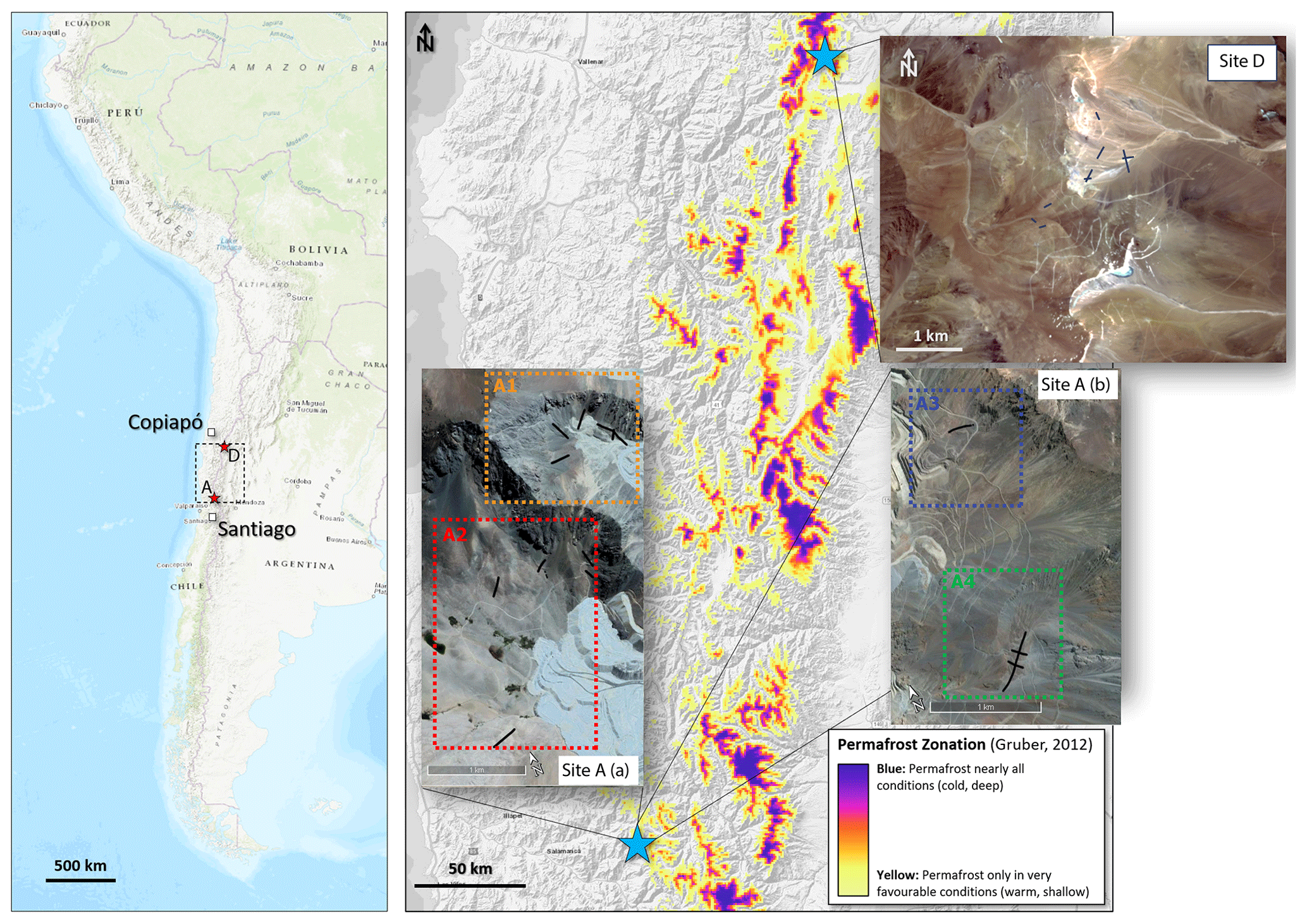
Figure 1 Overview maps of study sites A (rock-glacier-dominated site, including various sub-study areas A1–A4) and D (rock-glacier-free site) in the Central Andes of Chile and Argentina. The permafrost zonation index following Gruber (2012) shows the modeled permafrost distribution within the Central Andes. Black lines indicate the position of the geophysical profiles. Map data: Site A: Google, © 2022, Maxar Technologies; Site D: DigitalGlobe, accessed in Global Mapper V22 (Blue Marble Geographics), date unknown.

2.1 Rock-glacier-free site – Site D

The rock-glacier-free site is located between 3800 and 5400 m a.s.l., about 140 km southeast of the city of Copiapó (see Site D in Fig. 1). The climate of Site D is classified as semi-arid, typical for the high-altitude Central Andes. Precipitation and relative humidity are low, while solar radiation is high. Mean annual air temperature (MAAT) calculated from a meteorological weather station that was installed on site at an altitude of 5012 m a.s.l. in 2015 is −5.4 ^∘C (for the measurement period of 2015–2017). Using long-term representative regional climate stations in the vicinity of the site, a MAAT of −7.3 ^∘C was estimated for the period of 1978 to 2015. Mean annual precipitation estimated from the same long-term series is 131 mm, with significant variability (annual values ranging from 0 to 738 mm) (Devine et al., 2019). Site D is characterized by a uniform landscape consisting of a widespread fine-grained sediment cover. Rock glaciers are absent at this study site. Geomorphic surface indicators for permafrost mostly consist of widespread gelifluction lobes and in some cases weakly developed patterned ground.

The main host rock at Site D consists of Late Paleozoic (Permian–Triassic) rhyolites and andesites, which are overlain by Jurassic and Cretaceous sediments and conglomeratic clastic rocks that are strongly silicified and altered. Furthermore, Site D is located on a large hydrothermal alteration zone characterized by high sulfidation epithermal alterations and porphyry alterations. The bedrock is in general highly fractured as a result of the numerous fault systems that cross the area (Devine et al., 2019). The results of the geophysical surveys presented in Part 1 (see Hilbich et al., 2022a) point to largely homogeneous subsurface conditions with significant ground ice occurrences (mostly in terms of a thin, ice-rich layer varying in thicknesses of approximately 2–5 m). Furthermore, ground ice is expected to be present as well in the highly fractured and hydrothermally altered bedrock at greater depths (Hilbich and Hauck, 2018).

2.2 Rock-glacier-dominated site – Site A

Contrasting Site D, we choose a second field site with an abundance of specific permafrost landforms including rock glaciers and talus slopes. Site A is located in the upper part of the Choapa Valley, about 200 km north of Santiago de Chile (Fig. 1), and was previously studied by Monnier and Kinnard (2013). The geophysical measurements are located at an altitudinal range of 3560 to 3850 m a.s.l., whereas the maximum altitude of Site A is around 4300 m a.s.l. The climate of site A is semi-arid with a short rainy season between May and August. The annual precipitation ranges between 200 and 800 mm with an average of 334 mm for the period of 1961–1990. MAAT is estimated to be around +0.5 ^∘C in 2010 at an altitude of 3700 m a.s.l., which is a clear indicator that permafrost would not form under current climatic conditions and is naturally in a degrading state (Monnier and Kinnard, 2013). The most important periglacial landforms present at Site A are rock glaciers with about 15 rock glaciers that have been identified in the area of interest. Variable ground ice contents were found in the different rock glaciers and other landforms of Site A (Hilbich et al., 2022a; Monnier and Kinnard, 2013). Areas outside of rock glaciers are most likely unfrozen and free of permafrost, as seen by the relatively low electrical resistivities found in such areas (Hauck et al., 2017; Hilbich et al., 2022a) and as confirmed by several test pits.

The geology of Site A is characterized by volcanic (both intrusive and extrusive) and sedimentary rocks aging from the Middle Triassic until recently. A large part of the study area has been mapped as quartz diorites and andesites. Quaternary deposits consist of fluvioglacial sediments and morainic deposits. Similar to Site D, several faults associated with alteration and mineralization are located at Site A (Tapia et al., 2016).

3 Methods

The data sets used for this study consist of (i) geophysical measurements (electrical resistivity tomography, ERT, and refraction seismic tomography, RST), which are part of the large data set presented in the companion paper of Hilbich et al. (2022a), (ii) ground truth data in the form of test pits, boreholes, and natural outcrops (unpublished data provided by BGC Engineering Inc.: BGC), and (iii) geomorphological maps produced during fieldwork in the framework of this study. All data are then combined within a workflow for upscaling from the individual geophysical profile to the catchment scale (Fig. 2). The upscaling approach is based on the assumption that the geophysical profiles can be considered representative for larger areas with comparable near-surface substrate or for similar landforms in similar topo-climatic locations – by this representing comparable permafrost occurrences with similar ground ice contents. The workflow consists of five steps (Fig. 2): (1) creating a background permafrost distribution model, (2) modeling quantitative ground ice contents for each profile, (3) partitioning of the study site into different upscaling classes, and (4) establishing a conceptual soil stratigraphy model for each upscaling class. In a final step (5), the ground ice content estimates are upscaled to the whole study area using the upscaling classes as a basis. While steps (2) and (4) are closely related to the geophysical data and corresponding ground ice content calculations (see Sect. 3.1), steps (1) and (3) are more flexible and can be based on different approaches. Any permafrost distribution model may be used to distinguish between permafrost classes and non-permafrost classes (1), and any field information and remote sensing data can be used to classify the surface into upscaling classes (3). In the following, the different steps of the strategy are further explained before we show the results for the study site classification and the ice content quantification in the “Results” section (Sect. 4).

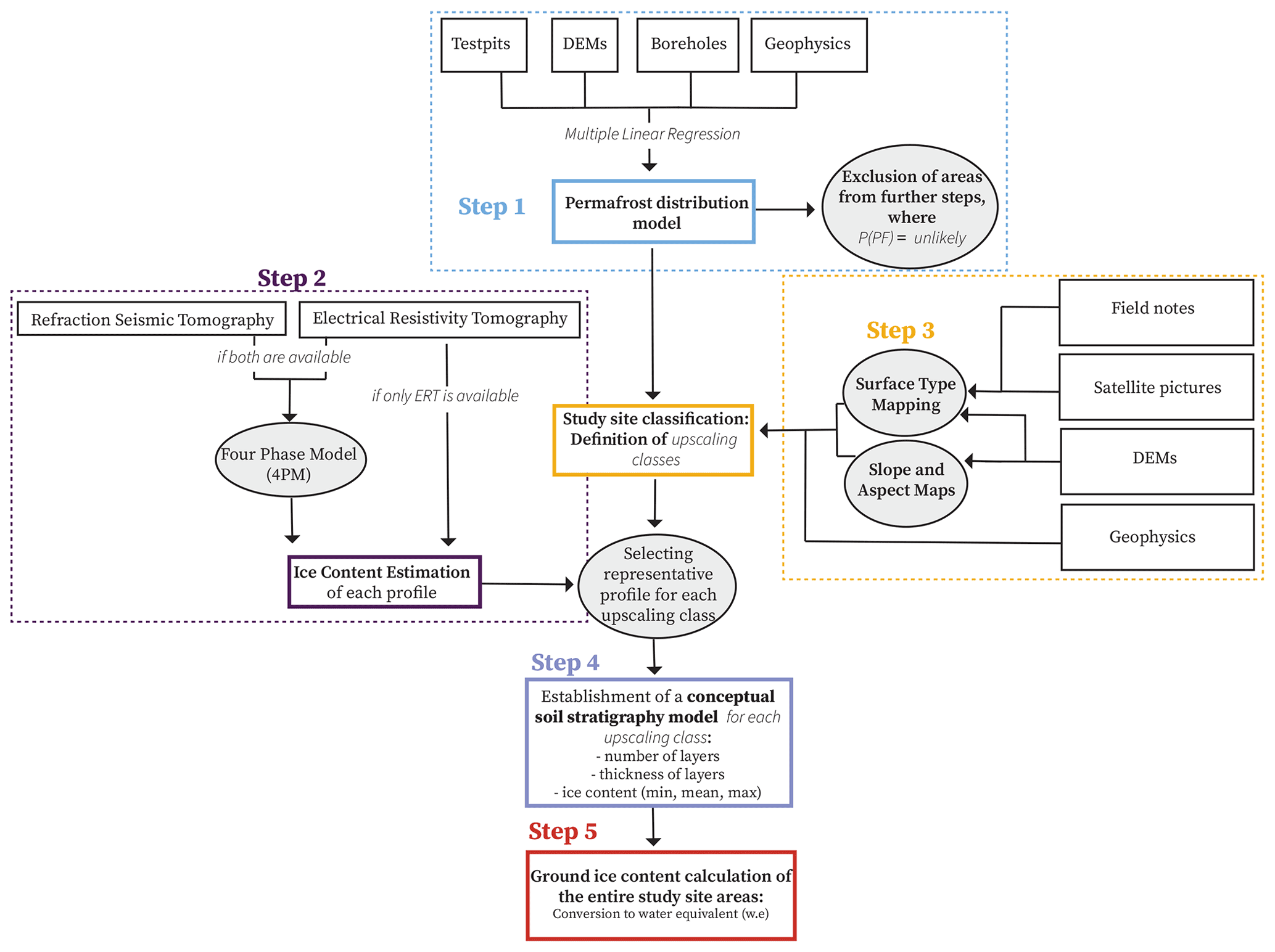
Figure 2 Workflow of the upscaling strategy used in this study. In step 1, we create a simple permafrost distribution model to exclude areas with low permafrost probability from further processing. Then, we use geophysical data and, where applicable, model the ground ice content using the 4PM (step 2). Then, in step 3, we define upscaling classes using information from different sources such as aspect and slope maps derived from DEMs, field notes, and observations. In step 4, a conceptual soil stratigraphy model is established using the geophysical results as input for subsurface layers and corresponding ice contents for each upscaling class, which serves as the basis for the upscaling of the ice content to the catchment scale (step 5).

3.1 Geophysical data sets and validation

In Part 1 of this study, Hilbich et al. (2022a) provide the details about geophysical data acquisition and processing, as well as data interpretation and ice content modeling, in the context of a comparison of several permafrost field sites in the Central Andes. It has to be noted that the geophysical profiles were not planned specifically for the purpose of upscaling to larger regions. However, the extensive data set allowed us to develop our strategy and apply it to the two field sites described above. Several sources of ground truthing were available for the validation of the geophysical results. At Site A, a large set of borehole data exist (Koenig et al., 2019), and the results from the geophysical surveys are in good agreement with the available borehole data (Hilbich et al., 2022a; Hauck et al., 2017; Hilbich and Hauck, 2018). At Site D, no geotechnical boreholes exist for calibrating the geophysical lines. However, several test pits were excavated, which largely confirmed the findings from the geophysical surveys. Additionally, several natural outcrops were present in the vicinity of the profiles and further served as validation data (Hauck et al., 2017; Hilbich and Hauck, 2018). Ground truthing data locations are shown in Fig. 3.

3.2 Permafrost distribution models

For the sake of simplicity and to use our available ground truthing data effectively, we chose a multiple regression approach that was first introduced by Hoelzle (1994) to generate a permafrost distribution model for our field sites. In contrast to, for example, Hoelzle (1994), who used data from the bottom temperature of the snow cover, we use the geophysical results, boreholes, and test pits as point input for the response variable Y, indicating likely permafrost occurrence or absence. Elevation and potential incoming solar radiation (PISR) were chosen as the predictor variables (Eq. 1). PISR was calculated using ArcGIS Pro's “Area Solar Radiation (Spatial Analyst)” tool, which uses a digital elevation model (DEM) as input and includes the latitude of the study sites for calculations of solar declination and solar position to derive PISR. In total, 50 point indicators for permafrost occurrence were used for the regression models. For Site D, these points correspond to either a location on a geophysical profile or a test pit located at elevations ranging from 4400 to 5151 m a.s.l. and comprise both permafrost and non-permafrost observations. A standard error of 0.58 and an R² of 0.6 were calculated. For Site A, point indicators correspond to points on the geophysical profiles or data from boreholes ranging from 3200 to 4000 m a.s.l. A standard error of 0.25 and R² of 0.72 were calculated. These regression statistics resemble the values used for models in other studies (e.g., Hoelzle, 1994) and are therefore considered to be acceptable.

$$\begin{array}{}\text{(1)}& y\left(x\right)=b_{\mathrm{0}}+b_{\mathrm{1}}\cdot \text{elevation}\left(x\right)+b_{\mathrm{2}}\cdot \text{PISR}\left(x\right),\end{array}$$

where b₀, b₁, and b₂ are regression coefficients.

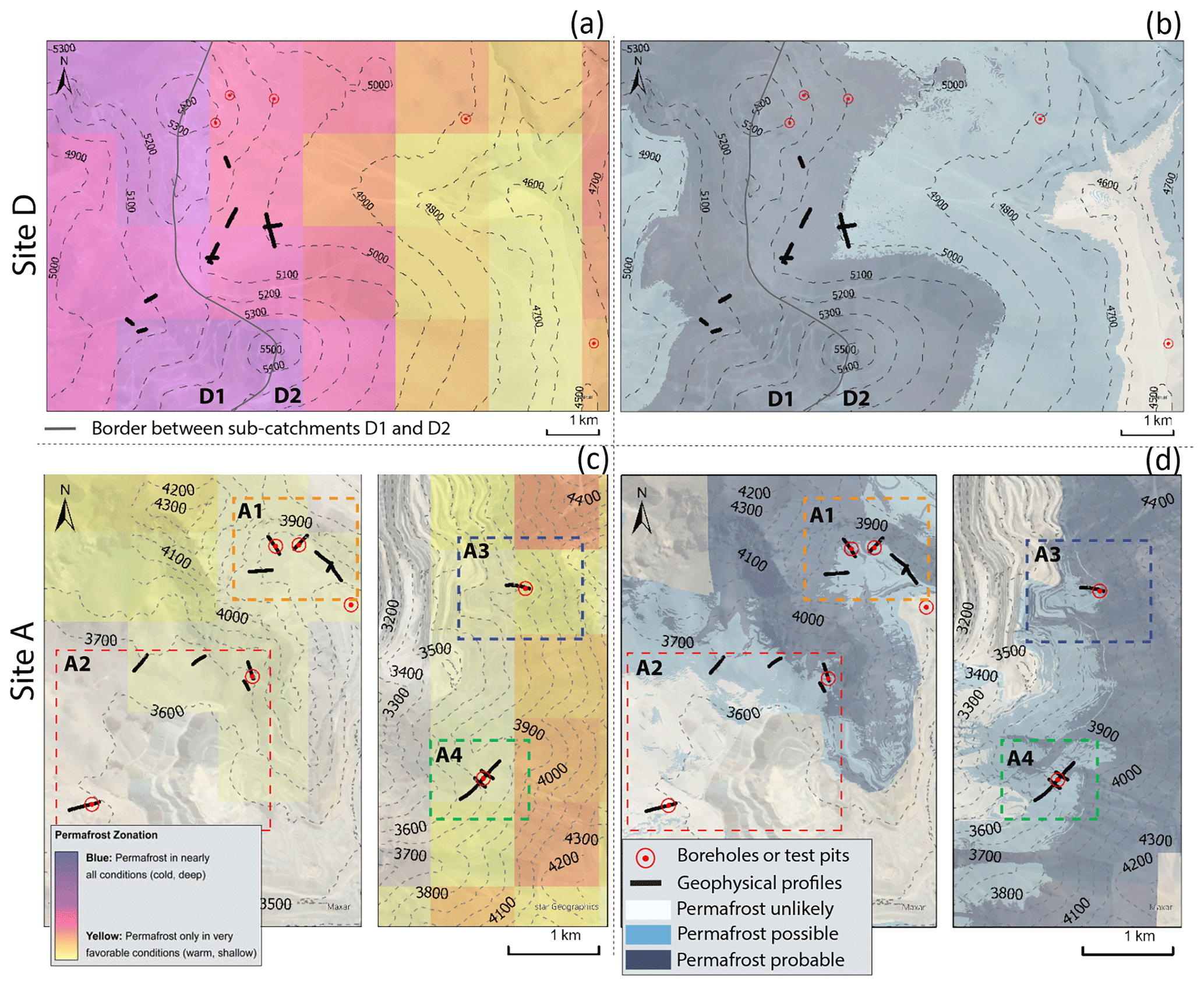
Figure 3 Comparison of the permafrost distribution model developed in this study (b, d; DEM 5 m resolution) with the PZI model by Gruber (2012) (a, c; based on SRTM30 data set, <1 km resolution). Locations of boreholes (Site A) and test pits (Site D) are marked by red points on all maps. Map data: DigitalGlobe, accessed in Global Mapper V22 (Blue Marble Geographics), date unknown.

The resulting permafrost distribution model delineates areas where permafrost occurrence is probable, possible, or unlikely, analogous to similar approaches in earlier studies (Hoelzle, 1994; Gruber and Hoelzle, 2001; Arenson and Jakob, 2010; Esper Angillieri, 2017; Kenner et al., 2019). The main purpose of the model in the context of this study is to provide a coarse overview of the expected permafrost distribution of the study region to be able to directly exclude those areas from further processing, where permafrost is highly unlikely (see white areas in Fig. 3b and d). More complex statistical permafrost distribution models for the Central Andes have been presented (e.g., Bodin et al., 2010; Azócar et al., 2017). However, they cover only parts of our study sites. A comparison of our approach with the model by Azócar et al. (2017) for Site A and with an unpublished model (Lukas U. Arenson Arenson, personal communication, 2018) following the approach presented in Arenson and Jakob (2010) for Site D showed a good agreement regarding the areas where permafrost is estimated to be absent. A comparison between the permafrost distribution model developed in this study and the global permafrost zonation index (PZI) developed by Gruber (2012) is shown in Fig. 3. For Site D, both models predict (high) probability for permafrost occurrence at the location of the geophysical profiles (black lines in Fig. 3). For Site A, the PZI does not cover the entire study site area, probably as a result of the lower altitude which is not taken into account in the PZI. At this site, the PZI predicts a low probability for permafrost occurrence at all subsites. The model developed in this study also delimits large portions of the study site as unlikely for permafrost. Nevertheless, it also suggests the possibility of permafrost (light blue areas) for most of the areas where the geophysical profile lines are located. A higher probability for permafrost is only modeled for steep and high altitude (>3800 m a.s.l.) bedrock slopes here. As a consequence of these clear differences between the two sites, the entire area of Site D was considered for the following steps of the strategy, whereas only rock glaciers and talus slopes were considered at Site A.

3.3 Study site classification

After excluding areas where permafrost is highly unlikely based on the distribution model, the study sites are subdivided and categorized into different classes, which are hereafter called upscaling classes. These classes are later used to upscale the estimated ground ice content from the geophysical profiles to a larger area. Surface characteristics are suitable data sets for upscaling approaches of geophysical data because the classification can be performed over larger areas using remote sensing data (e.g., Dafflon et al., 2017). In general, we distinguished different upscaling classes based on factors that are known to strongly influence the thermal regime of high mountain permafrost. The main classification criterion is the near-surface substrate type (e.g., coarse-blocky, fine-grained sediment) as it has been confirmed to be an important factor for the thermal regime and thus permafrost occurrence besides topo-climatic factors. For example, higher ground ice contents have been shown to be present in areas with blocky surface and subsurface material (e.g., Schneider et al., 2012; Staub, 2015; Gubler et al., 2013). Further, the presence of specific landforms such as active and relict rock glaciers, talus slopes, or gelifluction lobes is used as an important geomorphic indicator for permafrost and ice-rich zones as they have been shown to possess similar ground ice characteristics for a given region (see Hilbich et al., 2022a).

In addition, a good general understanding of the study site through field observations and any additional field data will strongly support the classification process, especially in heterogeneous mountain terrain. For Site D, a few general observations made on site and through the analysis of the geophysical data were used to define the upscaling classes, as well as the choice of the conceptual models and the ground ice content estimations described in the following section. At Site D, bedrock, as observed in outcrops during the field campaign, is highly fractured and ice-rich; frozen conditions can be assumed for greater depths and were also observed close to the surface (e.g., shallow active layer) in the various outcrops throughout the study site (Hilbich et al., 2022a). Likewise, field observations and the geophysical results have shown that the surface and the subsurface conditions are typically homogeneous. Frozen conditions can therefore be assumed for the entire study site. The resulting classes are further divided into smaller areas with presumably similar ground ice contents based on the results of the geophysical surveys and considering the exposition (aspect) of the area. A complete explanation of the different steps taken during the classification process is given in Sect. 4.1.

3.4 Quantification of ground ice contents per class

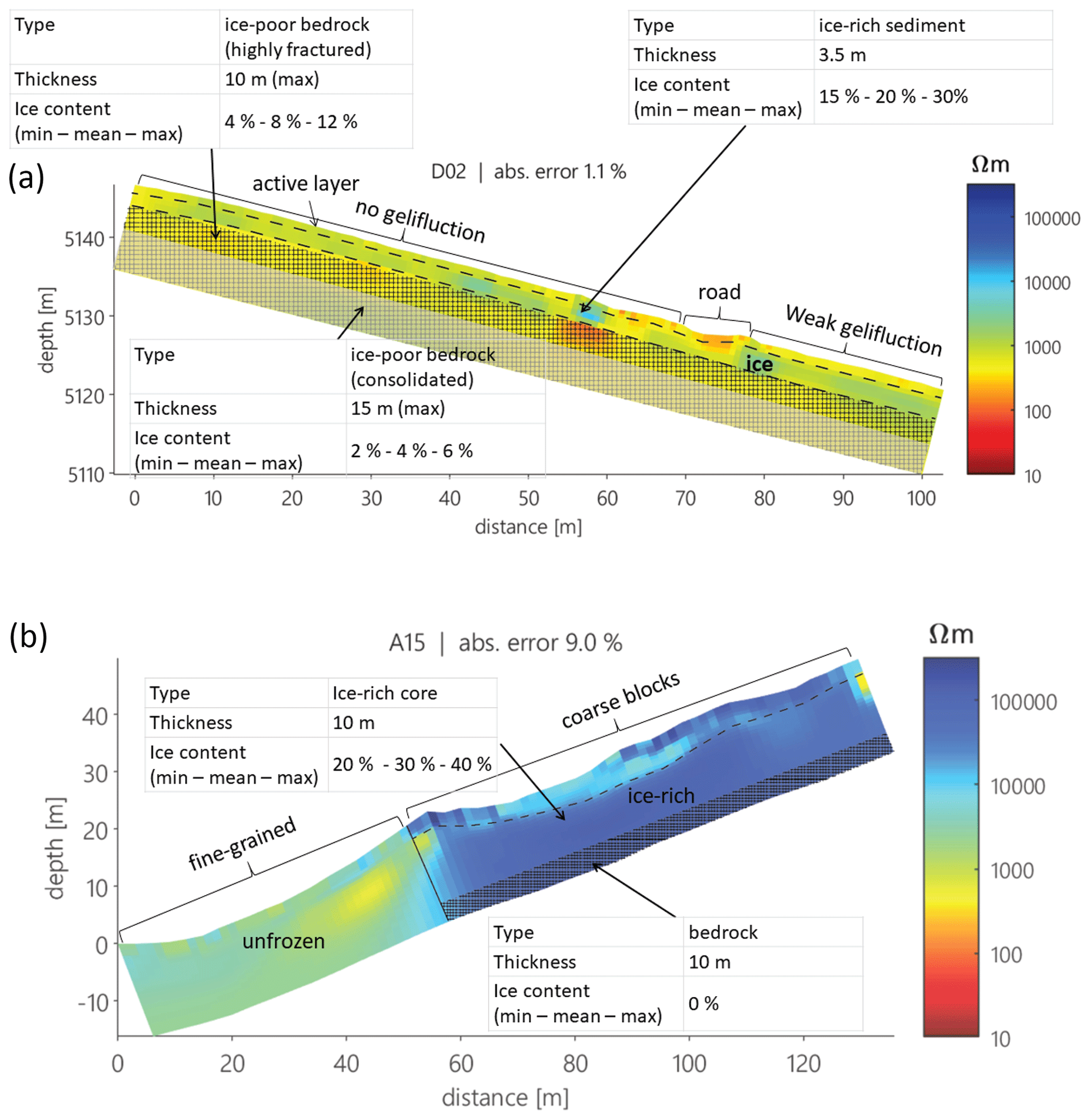
Figure 4 Examples of simplified soil stratigraphy models from both study sites (a: Site D; b: Site A). In both cases 4PM results are not available, and ground ice contents for the different layers are estimated from the ERT tomogram and based on ground truthing from test pits and outcrops.

For each upscaling class, a conceptual soil stratigraphy model was developed to further simplify the complex subsurface conditions into layered models with varying ground ice contents. These conceptual stratigraphies represent a simplified version of representative ERT tomograms. They form the basis for the upscaling of the ground ice content to the entire study site. Where available, the 4PM results are used for the estimation of the ice content of each layer. Where RST data and hence 4PM calculations are not available, estimations are based on an interpretation of the resistivity distribution of the subsurface alone, in combination with ground truthing data. Figures 4 and 5 show examples of such soil stratigraphy models for both study sites and both cases (with and without coincident RST data). The total ground ice content (in %) was then calculated using Eq. (2), which calculates the sum of the ground ice content X_i within each of the (total number of n) identified subsurface layers (i):

$$\begin{array}{}\text{(2)}& \sum _{i=\mathrm{1}}^n{X}_{\mathrm{i}}=(d\times A\times \text{ice}),\end{array}$$

where d is depth (m), A is area (m²), and ice is ice content (%).

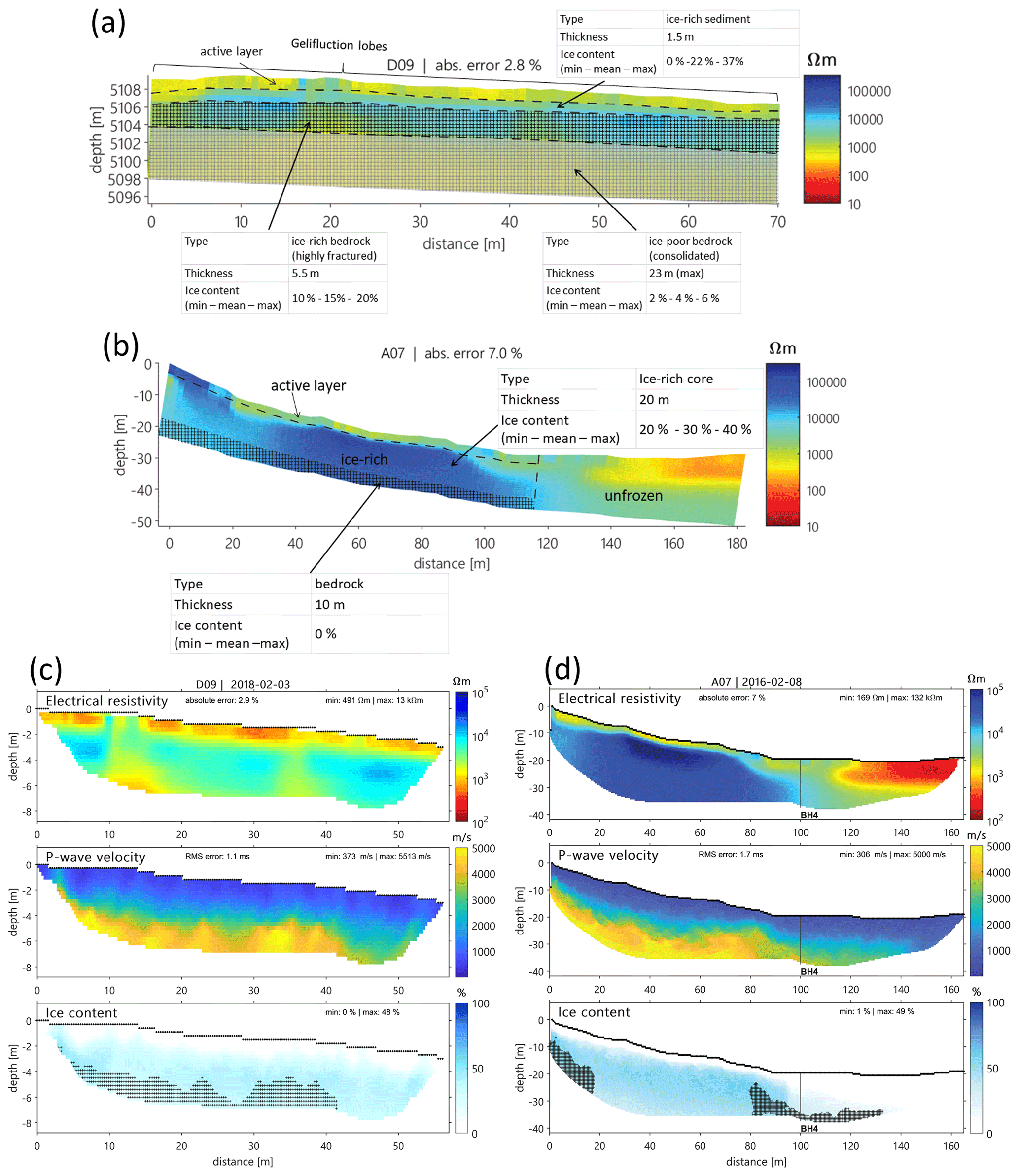
Figure 5 Examples of soil stratigraphy models for both study sites where the 4PM was applied. (a, b) Soil stratigraphy models and (c, d) corresponding 4PM results (ERT, RST, and ice content) (Hilbich et al., 2018). Here, ground ice content estimations stem from the 4PM results: the ice content values for the ice-rich layers correspond to the results from Part 1 of this study (Hilbich et al., 2022a). Ice content estimations for layers that are not considered in detail in Part 1 are mean values from the 4PM results (see Hilbich and Hauck, 2018; Hilbich et al., 2018).

A minimum, mean, and maximum ground ice content was considered for each layer in order to account for the uncertainties resulting from the approximation of a homogeneous thickness, area and ice content of each layer. For the (ice-rich) layers we use the same minimum, mean, and maximum ice content estimates as applied in the so-called zone of interest (ZOI) in Part 1 of this study (Hilbich et al., 2022a). Ice content estimations for layers that are not considered in detail in Part 1 are mean values from the 4PM results (see Hilbich and Hauck, 2018; Hilbich et al., 2018). Finally, the water equivalent (w.e.) was calculated for both sites assuming an ice density conversion factor of 0.9 g cm⁻³ (e.g., Paterson, 1994).

4 Results

The approach was applied to both study sites in order to test it for two cases that differ significantly in their surface and subsurface characteristics and corresponding permafrost distribution and conditions. As can be seen from the permafrost distribution models (Fig. 3), Site D is located in a zone with high permafrost probability and significant potential for the occurrence of ground ice (Fig. 3a and b) despite the absence of ice-rich landforms such as rock glaciers. On the contrary, permafrost ground ice is limited to rock glaciers and possibly talus slopes at Site A (see Fig. 3c and d).

For both sites, we calculated total volumetric ground ice estimates (Sect. 4.2) according to two different scenarios (S) with different assumptions regarding the spatial extent of ice-bearing layers for each site. For Site D, the two scenarios differ with respect to their investigation depths.

• SD1. Ground ice content contained in the uppermost 10 m is calculated. This scenario gives a relatively good estimate for the ground ice content in the near-surface layer of the study site, where the reliability of the geophysical surveys is high.

• SD2. The ground ice content down to a maximum depth of 30 m is calculated. Obviously, in areas with potentially deep permafrost occurrences, the total estimated ground ice content volume depends on the depth considered. This second scenario considers a greater investigation depth, which corresponds to 3 times the extent of scenario SD1 and may be more relevant for modeling purposes in the context of permafrost degradation and its impact on the water balance. Frozen ground conditions to even greater depths can be assumed for Site D; however, uncertainties regarding subsurface conditions (porosity, ice content, etc.) at greater depths are high.

For the rock glacier Site A, where permafrost is limited to rock glaciers and possibly talus slopes, the following scenarios were considered.

• SA1. The ice content of each sub-catchment is calculated by only considering the identified rock glaciers.

• SA2. This is like SA1 but includes talus slopes as additional potentially ice-rich landforms due to their coarse-blocky surface layer.

In the following sections, we will illustrate the individual steps of the upscaling strategy in detail mainly for Site D. However, the fundamental differences in ground ice distribution of the sites result in slightly different upscaling approaches for Site A and Site D. Therefore, we will also briefly explain the most important assumptions made for the ground ice content quantification of Site A.

4.1 Classification into upscaling classes

The upscaling classes determined for Site D are listed in Table 1, together with their specific surface characteristics, permafrost probability, aspect, and the tomogram representative for each upscaling class. These ERT tomograms can be found in the Appendix (Fig. A1). For a more detailed discussion of the individual ERT and RST tomograms see Hilbich et al. (2022a) and Hilbich and Hauck (2018).

Table 1 Definition of the upscaling classes used for Site D.

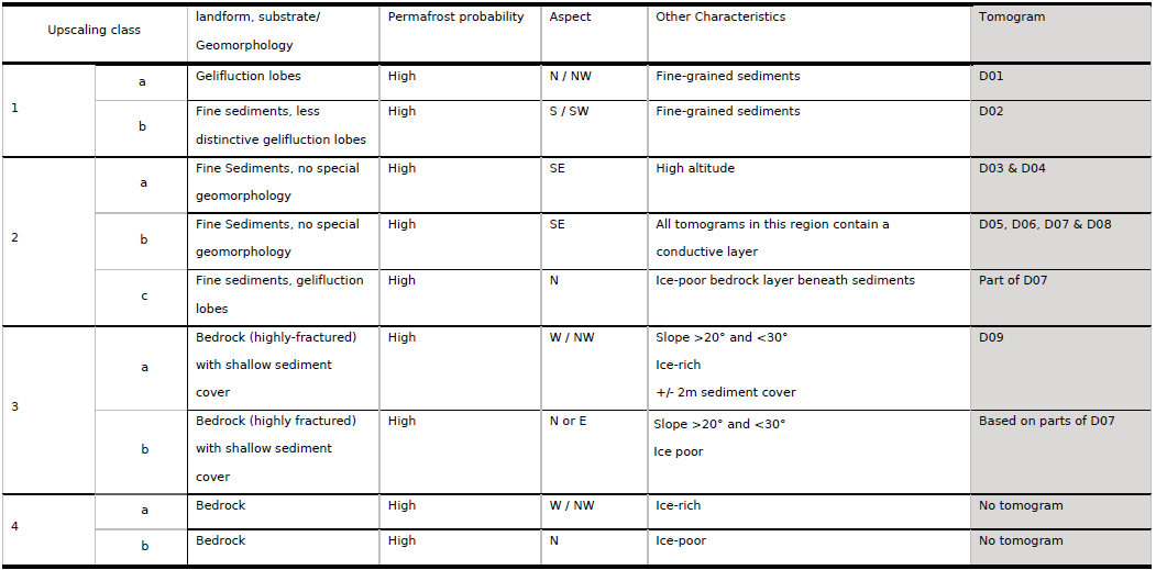
For the classification, Site D was split into sub-catchment D1 to the west of the main ridge and sub-catchment D2 located to the east (Fig. 6). For the classification, the surface types and landforms were mapped manually based on satellite images and geomorphological mapping during the field campaigns and using a DEM to delimit bedrock areas based on a slope threshold. At Site D surface types and landforms include fine-grained (colluvial) sediments, gelifluction lobes, bedrock with a sediment veneer (defined as approximately <2 m sediment covering the bedrock), and pure bedrock. Sub-catchment D1 is characterized by a widespread fine-grained sediment cover. The sub-catchment is further divided into (a) the northwestern slope with fine-grained sediment and gelifluction lobes (upscaling class 1a, with D01 serving as reference tomogram) and (b) the southwestern slope dominated by fine-grained sediment without gelifluction lobes (upscaling class 1b, with D02 serving as reference tomogram). Profile D09 serves as reference for slopes steeper than 20^∘ which were classified as bedrock with a thin sediment cover (sediment veneer) based on field observations and defined as upscaling class 3a. Hereby, a thin sediment layer of 1.5–2 m above a highly fractured, likely ice-rich bedrock was observed at an outcrop close to profile D09. The area of sub-catchment D1 with slope angles >30^∘ is mapped as pure bedrock (upscaling class 4a). This threshold is based on field observations and mapping, where an absence of significant sediment covers were observed in areas steeper than 30^∘. It is assumed to be ice-rich in the uppermost layer and ice-poor at greater depths, further considering the results of profile D09. A large central area of sub-catchment D2 consists of colluvial, fine-grained sediment that does not contain any specific landform. Profiles D03, D04, D05, D06, D07, and D08 are all located in this area (Fig. 6). The results from the geophysical surveys point to differences between the profiles located at lower elevations (in the center of sub-catchment D2) and profiles located higher up in steeper slopes. Therefore, this colluvial, fine-grained sediment area was further subdivided into upscaling classes 2a and 2b. Zone 2a contains the profiles D05, D06, D07, and D08, which are all characterized by a distinctive conductive layer whose thickness is probably overestimated by the inversion process (see Part 1 of this contribution, Hilbich et al., 2022a). Zone 2b hosts the profiles D03 and D04, which do not contain said conductive layer. At the foot of the local mountain peak gelifluction lobes were observed during the field work (Zone 2c). Profile D07, which reaches the lower boundary of these gelifluction lobes, may point to less ice-rich bedrock conditions compared to what has been found in D09 in sub-catchment D1. Thus, the right-hand part of D07 is taken as a reference for the ground ice calculations for this area, defined as Zone 2c. Similar to sub-catchment D1, slopes steeper than 20^∘ were mapped as bedrock with a shallow sediment cover. This concerns a small section (Zone 3b₂) next to Zone 2b but mostly the northern slope of the local mountain peak. Because of its northern aspect and resulting higher exposure to solar radiation, this area (Zone 3b₁) is assumed to be less ice-rich than its mostly western–northwestern-facing counterpart in sub-catchment D1. The steepest slopes (>30^∘) located at the top of the peak in the southeast were mapped as pure bedrock (Zone 4b). Following the argumentation for Zone 3b, this area is also considered to be less ice-rich than the pure bedrock of sub-catchment D1.

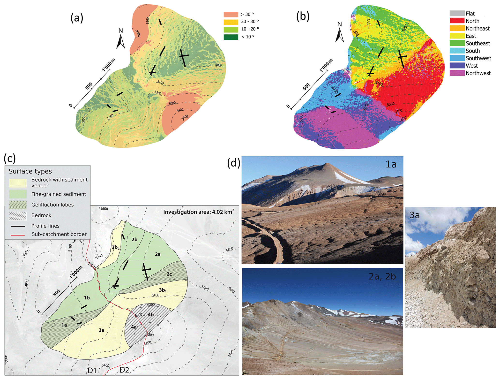
Figure 6 Map showing the different upscaling class areas for Site D (c). The photographs (d) illustrate the general surface types for some of the most important upscaling classes (highly fractured bedrock (3a), widespread uniform fine-grained sediment (2a, 2b), and gelifluction lobes (1a)). Also shown are the slope (a) and aspect (b) maps used for the study site classification. Map data: DigitalGlobe, accessed in Global Mapper V22 (Blue Marble Geographics), date unknown.

The geomorphological mapping and classification for Site A (not shown in the scope of this paper) yielded areas of fine-grained sediments with slopes <20^∘ (Class 1), bedrock with a shallow sediment cover (Class 2) (slope >20 and <30^∘), and pure bedrock (Class 3) (slopes >30^∘), in addition to the mapped rock glaciers and talus slopes for each sub-catchment. However, as the permafrost distribution modeling showed that permafrost can be assumed to be absent outside of rock glaciers and talus slopes at Site A, the resulting upscaling classes containing ice only include rock glaciers (scenario SA1) or rock glaciers and talus slopes (scenario SA2). Each rock glacier for which the ice content was modeled using the 4PM is considered its own upscaling class (Class 4x) with a specific subsurface soil stratigraphy and ice content, accounting for their heterogeneity which was observed through the geophysical surveys. Rock glacier areas without geophysical measurements were first categorized as intact (Class 5, potentially ice-rich) or relict (Class 6, unfrozen) using the rock glacier classification made by Azócar et al. (2017). Talus slope areas were divided into two upscaling classes, differing between north- (Class 7) and south-facing slopes (Class 8), to account for possibly lower ice contents in north-facing slopes.

The classification process can be summarized by the following steps.

1. Areas (polygons) with slopes >30^∘ are identified and isolated using a DEM (5 m resolution) to map bedrock areas, as well as slopes with >20^∘ and <30^∘ to map bedrock with a sediment veneer.

2. Any other surface types and landforms observed in the field and on satellite pictures are mapped.

3. The geophysical results for the different surface types and landforms are checked, if available. If more than one geophysical profile is present for one surface type class in a sub-catchment (e.g., the fine-grained sediment area in the center of sub-catchment D2), the profiles are checked for whether they suggest homogeneous subsurface conditions for the surface type class or not.

4. If the profiles do not suggest homogeneous subsurface conditions, the area is further subdivided into smaller upscaling classes. For this, any additional available information that can be used to explain the differences seen in the geophysical results can be used.

5. If no geophysical profile is present in a delimited area (e.g., upscaling class 3b₁,₂ in sub-catchment D2), the information for the subsurface conditions is taken from a profile with similar surface conditions (surface type, altitude, etc.). Here, we again rely strongly on field observations and expert knowledge in order to choose the most representative profile for the definition of the subsurface stratigraphy and ice contents.

6. Finally, a soil stratigraphy model is established for each upscaling class based on the representative geophysical profile chosen in points 2–4.

4.2 Ground ice content quantification

The ground ice content was quantified for each upscaling class based on the conceptual soil stratigraphy models (see Figs. 4, 5). To do this, Site A was partitioned into smaller sub-catchments as a result of its larger size in comparison to Site D. The partitioning into A1, A2, and A3/4 is a function of the spatial “clustering” of geophysical profiles at Site A. Site D was not further subdivided for the calculation of the total ground ice contents and water equivalents as the total area is comparatively small and because the geophysical profiles are located in closer proximity. In cases where (i) geophysical profiles are not available, (ii) the investigation depth of the geophysical surveys is insufficient, or (iii) certain layer boundaries could not be resolved, additional assumptions had to be made for individual layers of the upscaling classes. Table 2 summarizes the generalized layer structure (active layer, ice-rich sediment layer, and bedrock layer), including maximum thicknesses and mean ice contents for such cases at Site D.

Table 2 General assumptions of layers used in the conceptual soil stratigraphy models for the ground ice content calculations for Site D, where (i) no 4PM results exist, (ii) ground truthing data are absent, and/or (iii) the investigation depth from the geophysical methods is not sufficient.

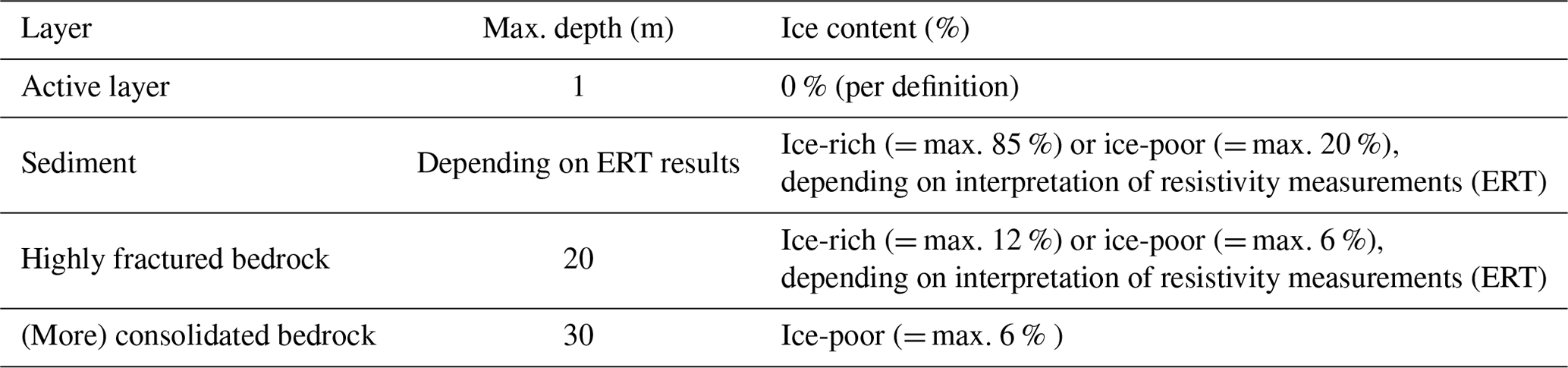
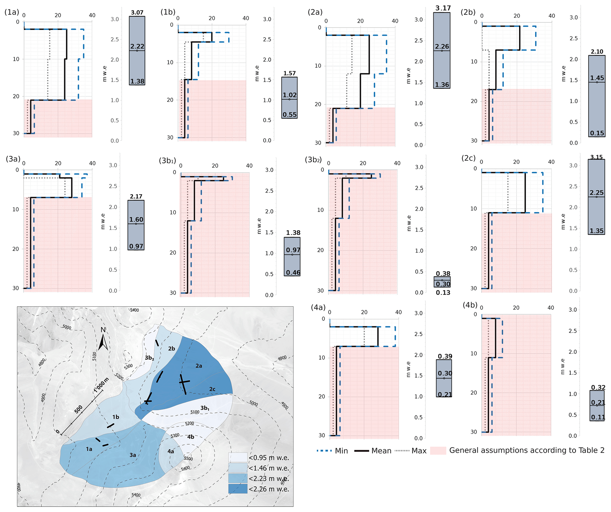
Figure 7 Assumed min, mean, and max ice content stratigraphies for all upscaling classes (x axis = ice content (%), y axis = depth (m)), based on the geophysical results and calculated ground ice content for each upscaling class. The red shaded parts of the plots indicate where assumptions were made based on Table 2. The resulting min, mean, and max water contents for each class are shown (in m w.e.) in the boxplots. The map shows the meters of water equivalent distribution for site D.

For Site A, ground ice contents for the ice-rich core of rock glaciers (Class 4x) were taken from the 4PM results where available, as published in Hilbich et al. (2022a). The bedrock below the frozen layer is assumed to be unfrozen in the entire study area. Where no geophysical measurements are available for ice content estimations, the ice content of the ice-rich core of intact rock glaciers (Class 5) is derived using average values for rock glaciers that are situated in similar settings (aspect, altitude, permafrost probability) at Site A. Relict rock glaciers (Class 6) are considered to not contain ground ice anymore. For scenario SA2, talus slopes were furthermore considered to contain possible ice-bearing layers (Gude et al., 2003; Hauck and Kneisel, 2008b; Mollaret et al., 2020). Here, we assume lower ice contents for north-facing talus slopes (Class 7) ranging from 0 % to 10 % than for south-facing slopes (Class 8), where we applied an ice content range of 5 % to 20 %. These assumptions stem from the hypothesis that talus slopes can potentially store significant ice volumes as a result of their blocky (insulating) surface layer that allows for more effective cooling (e.g., Wicky and Hauck, 2017). However, the geophysical and 4PM results on talus slopes presented in Part 1 of this study (Hilbich et al., 2022a) are not conclusive in terms of ice content. The numbers presented in this part of the study should, therefore, be viewed with care. More research is clearly needed to better estimate the ice content in talus slopes as the current data coverage is very scarce.

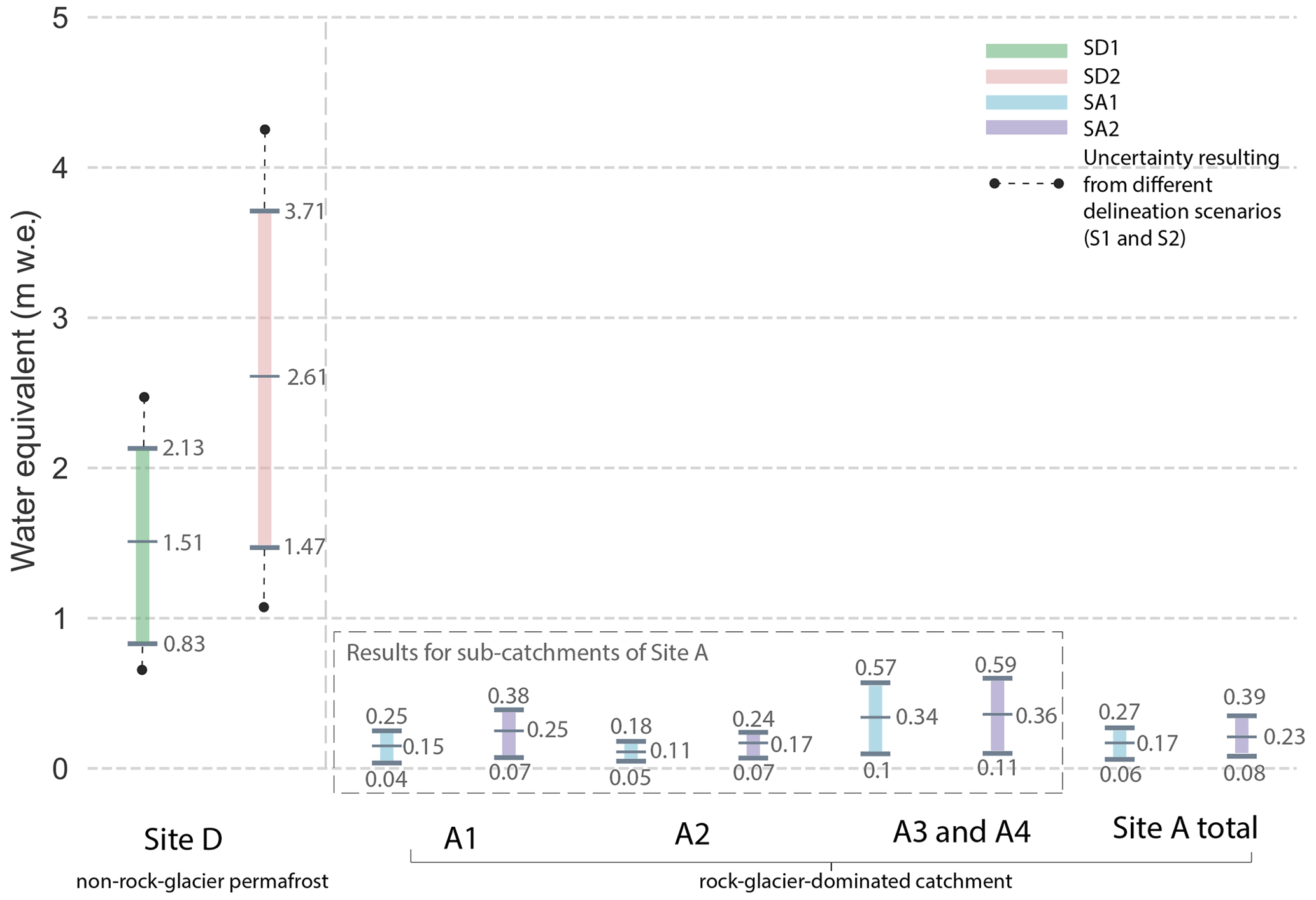
Figure 8 Calculated minimum, mean, and maximum water equivalents (m w.e.) for the different scenarios (SD1–SA2), as well as for rock glaciers and talus slopes, at Site A only. For SD1 and SD2, the black bars indicate the uncertainty resulting from using different delineation scenarios for the upscaling classes (see “Discussion”).

Figure 7 shows the ice content percentage profiles of the soil stratigraphies resulting from step 4 of our workflow (see Fig. 2) until a maximum depth of 30 m, together with the corresponding calculated water equivalents (min, mean, and max values) for each upscaling class for Site D. It also shows a map that indicates the distribution of meters of water equivalent in the study site. The calculated total ground ice contents per upscaling class were then summed up for the entire considered area and converted into water equivalents (m w.e.) (Fig. 8). The total ground ice volumes on the catchment scale calculated for Site D (total area of 4.02 km²) range between 0.0033 and 0.0085 km³ for an investigation depth of 10 m (scenario SD1) and 0.0059 and 0.015 km³ for an investigation depth of 30 m (scenario SD2). These results equal a water equivalent ranging from 0.83 to 2.13 m w.e. for a depth of 10 m and 1.47 to 3.71 m w.e. for the 30 m investigation depth. For Site A, the total ground ice volumes (for a total area of 15.32 km²) range between 0.0010 and 0.0047 km³ for scenario SA1 and 0.0013 and 0.006 km³ for scenario SA2. This equals a water equivalent of 0.06–0.27 m w.e. for SA1 and 0.084–0.39 m w.e. for SA2 (Fig. 8). Values for the Site A sub-catchments are in a similar range. Therefore, the permafrost ground ice volumes and corresponding water equivalents are substantially larger at Site D. This suggests that non-rock-glacier catchments may also contain substantial volumes of ground ice. It is, however, important to note that this ground ice does not necessarily influence the water balance and probably only marginally influences the annual watershed hydrology (see conclusion in Sect. 6).

Our results point to substantial ground ice occurrences outside of rock glaciers. In direct comparison to the rock glacier area of Site A, the total ice contents calculated for Site D contain only 10 %–20 % (for the 10 m investigation depth scenario) of the ground ice content stored in rock glaciers at Site A. However, on the catchment scale, when comparing water equivalents between Site A and Site D, the values for Site D are several times larger (Fig. 8). Based on water equivalents contained in the defined catchment areas, Site A (for scenario SA1) contains only about 7 %–12 % of what is stored at Site D for the 10 m depth scenario. This is considered reasonable as most of the catchment area of Site A (outside of rock glaciers) is expected to be unfrozen (permafrost-free).

5 Discussion

With the upscaling strategy established in the framework of this study, ground ice content estimations are now also possible outside of rock-glacier-dominated catchments, and the relative importance of different permafrost occurrences for total ground ice volumes can be evaluated. It is acknowledged that the absolute numbers of our results should be considered with care as there are many uncertainties involved in the various steps of our upscaling strategy. These uncertainties are discussed below.

• (i)

  The estimation of the ice content of the different layers in the conceptual soil stratigraphy models for each site is challenging as the prescription of a realistic porosity model is a known weakness of the geophysics-based four-phase model (4PM) (Mewes et al., 2017; Pellet et al., 2016). This has been addressed with the development of the so-called petrophysical joint inversion (PJI) scheme that is able to invert for porosity in addition to ice and water content (Wagner et al., 2019; Mollaret et al., 2020). However, the successful application of the PJI to a large number of geologically and geomorphologically different profiles is still difficult due to convergence problems in the absence of a priori knowledge (see Part 1, Hilbich et al., 2022a). For the calculations of this study, the porosity models were adjusted for each profile based on (a) the landform and the surface substrate, (b) the interpreted geophysical results, and (c) ground truthing information, where available. We assume porosity values around 50 % for the uppermost sediment layers at the sediment sites and around 40 % for highly fractured bedrock (with a decreasing gradient for more consolidated bedrock that is expected underneath). For the rock glaciers of Site A, porosity values >60 % were prescribed in the case of highly resistive layers to allow for supersaturated conditions (see Hilbich et al., 2022a). As these values are merely (field-based) assumptions, porosity estimates could be a source of uncertainty by leading to either over- or underestimation of the ground ice contents.

• (ii)

  Although capable of estimating ground ice content from the geophysical results (e.g., Pellet et al., 2016; Halla et al., 2021; Mollaret et al., 2019; de Pasquale et al., 2022), the success of the 4PM application depends on the available data. The identification of representative ground ice content of the different layers is therefore often not possible from the geophysical results alone. In addition, the 4PM requires co-located ERT and RST measurements, which are not always available in a sufficiently large number to be used in an upscaling approach as presented in our study.

• (iii)

  The conceptual soil stratigraphy models used here assume a constant thickness and ice content for the entire upscaling class (under the assumption of relatively homogeneous conditions at Site D). However, lateral differences are to be expected, and the derived ground ice content estimates can only serve as rough approximations on the catchment scale.

• (iv)

  There are also various uncertainties with regard to the classification of the study area into upscaling classes, especially where clear landforms (e.g., rock glaciers, talus slopes) are absent, as is the case for Site D. The classification process is of a rather qualitative nature and strongly relies on field observations and expert knowledge. The large potential uncertainties associated with the classification step are indicated by the uncertainty bars shown in Fig. 8. These large error bars originate from the uncertainties regarding the spatial extent of the upscaling classes and corresponding subsurface ice occurrences and their maximal/minimal values. To assess the sensitivity of the calculated ground ice contents to the delineation of the upscaling classes, different possible classification scenarios were compared for Site D. The scenarios were established by either using different tomograms as reference for the ice content of an upscaling class or by assuming more/fewer sub-classes (i.e., combining similar classes to larger upscaling classes or subdividing upscaling classes to smaller ones). The resulting ranges of the ground ice contents calculated for each scenario reach from 14 % to 28 % (shown by black bars for SD1 and SD2 in Fig. 8), with lower uncertainty ranges for the 10 m investigation depth. The uncertainty range shown in this figure represents the upper bound. In a purely applied study, one would narrow down this uncertainty range by choosing a best guess scenario for spatial extension, depth of layers, and ice content ranges.

To resume, the main uncertainties of the ice content estimation result from (a) the assumptions for min and max ice contents (partly related to uncertainties of the 4PM) and (b) the classification of the upscaling classes. Especially in catchments where landforms with clear morphological outlines are missing, the latter may cause substantial uncertainties regarding the spatial extension of the subsurface ice occurrences and their maximal or minimal ice content values. Nevertheless, wherever geophysical data are available in combination with the observations made during the field campaigns, we can be rather confident about the results for Site D for an investigation depth of 10 m (see comparison with ground truthing data in Part 1, Hilbich et al., 2022a). The 30 m depth scenario should be considered with more caution as it is close to the limit of the penetration depth of the available geophysical surveys.

Figure 9 Comparison of water equivalent (m w.e.) estimations for Site A, scenario SA1 (considering only rock glaciers as ice-bearing class), for (i) the geophysically based upscaling technique (blue bars) presented in this paper and (ii) the empirical rule (red bars) introduced by Brenning (2005).

To our knowledge, permafrost ground ice outside of rock glaciers has not yet been quantified or documented in discussions related to permafrost in the Andes. Most published studies on estimating the hydrological importance of rock glaciers in the Andes base their estimations of the thickness of the ice-rich layer on an empirical rule proposed by Brenning (2005) (e.g., Esper Angillieri, 2009; Rangecroft et al., 2015; Jones et al., 2018a, 2019). This empirical relation is based on rock glacier geometry obtained through geomorphological mapping and relates the thickness of the ice-rich layer to the rock glacier area without explicitly taking into account the potentially complex spatial variability and dependence on rock glacier kinematics and morphology. As shown by the extensive field-based data presented in the companion paper by Hilbich et al. (2022a), the resulting estimates of the thickness of the ice-rich layer of active rock glaciers is in most cases overestimated when compared to what has been estimated from geophysical surveys and boreholes. For some rock glaciers the empirical rule-based estimates of rock glacier thickness is twice as large as what has been found through the geophysical measurements, in which the thickness of a potentially ice-rich core can be delimited with high confidence due to the large resistivity contrasts between the different layers. In consequence, area–thickness-based calculations of ground ice volumes are significantly higher than calculations based on geophysics. The additional assumption of a general volumetric ice content of 50 % commonly used certainly adds to the overestimation of the ice volume contained in certain rock glaciers. Hilbich et al. (2022a) found that such previous ground ice content assumptions for rock glaciers correspond to field-based results only when their ice-rich zone alone is considered.

Figure 9 compares the results of the water equivalents for Site A, scenario SA1 (only considering rock glaciers), using our field-based upscaling approach with the total water equivalents calculated using the empirical approach by Brenning (2005), both per sub-catchment and for the total study site area. The geophysically based results are given as minimum, mean, and maximum ice content per subsurface layer, whereas we used minimum, mean, and maximum ice content assumptions of 20 %, 50 %, and 60 % in addition to the empirical thickness estimation of the ice-rich layer to illustrate the approach of Brenning (2005). As can be seen from Fig. 9, the mean water equivalent calculated using the empirical rule is much larger in all cases compared to the results using the geophysics-based upscaling technique of this study. Although acknowledging the fact that simplified empirical rules can be useful tools to cover large and remote areas, they clearly over-generalize the complex and heterogeneous subsurface conditions and ground ice contents of rock glaciers. We believe that using field-based evidence (such as geophysical investigations) in combination with large-scale remote sensing data ultimately leads to more realistic ground ice content quantification compared to purely remote sensing approaches. For Site A, we can be confident that ground ice quantification based on the large number of geophysical profiles carried out on the various rock glaciers are more realistic than the pure remote sensing estimates. Furthermore, with the geophysical data presented in Part 1 of this study (Hilbich et al., 2022a) it becomes clear that rock glacier ice contents may vary significantly from the commonly used 40 %–60 %. This is why our upscaling approach strongly relies on in situ data, although it means that it is not directly transferable to other catchments where no geophysical data exist. Nevertheless, we believe that field-based data (geophysical or other) are in any case essential for validating remote sensing products or model-based estimates on ground ice contents.

Even if the uncertainties remain considerable, the general permafrost distribution and the intra- and inter-landform heterogeneity of the considered catchments is much better captured by geophysical profiles than from remote-sensing-based approaches alone. This is especially important for catchments that do not contain any clear geomorphic permafrost indicators, such as rock glaciers, that could be delineated using remote sensing data.

6 Conclusion

In this paper we presented an upscaling strategy for geophysical measurements with the aim to characterize the subsurface conditions in high mountain areas with regard to the occurrence of permafrost. Further, the potential ground ice content for the entire area of two study sites was calculated. The study is based on a series of geophysical measurements (ERT and RST) that were carried out at several study sites in the dry Andes of Chile and Argentina (Central Andes), presented in Hilbich et al. (2022a), of which we apply our approach to one rock-glacier-dominated and one rock-glacier-free site. The upscaling method is based on (a) a simple statistical approach that follows previous work on permafrost distribution models, using the geophysical data as permafrost evidence, and (b) a linkage between geophysical results, substrate type, and surface geomorphology to define and delimit areas with presumably similar subsurface conditions (active layer thickness, ground ice content). The so-defined areas were used as upscaling classes and further used to calculate total ground ice volumes for a larger area. The general approach and strong linkage to the extensive geophysical data sets allowed the estimation of ground ice volumes on the catchment scale. An important advantage of our approach is that it is not restricted to rock glaciers, as in most studies present to date (Azócar and Brenning, 2010; Rangecroft et al., 2015; Schaffer et al., 2019; Jones et al., 2018b; Croce and Milana, 2002). We demonstrate that the estimation of large-scale ground ice volumes can be improved by including (i) non-rock-glacier permafrost occurrences and (ii) field evidence through a large number of geophysical surveys and ground truthing information (where available). The upscaling strategy presented in this paper is a first attempt at estimating ground ice contents on a larger scale than just landforms (e.g., rock glaciers or talus slopes). Based on our findings, further studies should focus on improving the knowledge of the ground ice content distribution in different landforms aside from rock glaciers. Furthermore, the upscaling approach could be improved by, for example, coupling the geophysical results to a spatially distributed ground thermal model or using machine learning to exploit relationships between surface and subsurface parameters. Our study presents one of the first estimations of the ground ice volume and corresponding water equivalents contained in ice-rich permafrost areas in rock-glacier-free catchments. It has been shown that such areas can contain a substantial volume of ground ice that should not be neglected in cryospheric, hydrologic, climate, or environmental studies. It is, however, important to note that the water, stored in the ground ice, does not necessarily influence the annual variability in the water balance as the presence or absence of a rock glacier in a watershed may only marginally influence the annual watershed hydrology. Other factors, such as the overall permafrost characteristics, terrain types, and precipitation patterns, play more significant roles. Therefore, without further investigations and especially the assessment of the temporal scales of runoff contribution of ground ice melt from such extensive permafrost occurrences, its importance for the hydrological cycle cannot be addressed.

Appendix A

Figure A1 Inverted tomograms of all ERT profiles for Site A and Site D.