Towards accurate quantification of ice content in permafrost of the Central Andes – Part 1: Geophysics-based estimates from three different regions

Increasing water scarcity in the Central Andes due to ongoing climate change recently caused a controversy and debate on the significance of permafrost occurrences for the hydrologic cycle. The lack of comprehensive field measurements and quantitative data on the local variability in internal structure and ground ice content further exacerbates the situation. We present field-based data from six extensive geophysical campaigns undertaken since 2016 in three different high-altitude regions of the Central Andes of Chile and Argentina (28 to 32^∘ S). Our data cover various permafrost landforms ranging from ice-poor bedrock to ice-rich rock glaciers and are complemented by ground truthing information from boreholes and numerous test pits near the geophysical profiles. In addition to determining the thickness of the potential ice-rich layers from the individual profiles, we also use a quantitative four-phase model to estimate the volumetric ground ice content in representative zones of the geophysical profiles. Our analysis of 52 geoelectrical and 24 refraction seismic profiles within this study confirmed that ice-rich permafrost is not restricted to rock glaciers but is also observed in non-rock-glacier permafrost slopes in the form of interstitial ice, as well as layers with excess ice, resulting in substantial ice contents. Consequently, non-rock-glacier permafrost landforms, whose role for local hydrology has so far not been considered in remote-sensing-based approaches, may be similarly relevant in terms of ground ice content on a catchment scale and should not be ignored when quantifying the potential hydrological significance of permafrost. We show that field-geophysics-based estimates of ground ice content, while more labour intensive, are considerably more accurate than remote sensing approaches. The geophysical data can then be further used in upscaling studies to the catchment scale in order to reliably estimate the hydrological significance of permafrost within a catchment.

1 Introduction

Permafrost covers about 15 % to 20 % of the Northern Hemisphere global land surface (Obu, 2021; Obu et al., 2019). Most permafrost studies address permafrost occurrences either in the Arctic, Antarctica, or mountain ranges of the Northern Hemisphere. However, in the mid-latitudes of the Southern Hemisphere the presence of permafrost is also widespread at high elevations in the Central Andes of South America, where only a few studies and even fewer borehole data (e.g. within the global permafrost data base GTN-P; Biskaborn et al., 2019) currently exist. Continued climate change is projected to cause significant temperature increase for the Subtropical Central Andes, yielding significant water shortage especially in the arid mountain regions (Hock et al., 2019). In this context, the significance of permafrost occurrences in the Central Andes for the hydrological cycle is currently controversial (e.g. Arenson and Jakob, 2010; Azócar and Brenning, 2010; Brenning, 2008; Duguay et al., 2015; Jones et al., 2019). On the one hand, permafrost in general and especially rock glaciers (which are conspicuous and often ice-rich permafrost landforms) are considered main storages of frozen water and alternative future water resources in view of the ongoing recession of glaciers in the Dry Andes (e.g. García et al., 2017; Masiokas et al., 2020; Rangecroft et al., 2015). Consequently, degrading permafrost is speculated to partly compensate for the strongly decreasing glacial discharge in the future and aid the strong demand for fresh water from the Andean Cordillera, caused by the growing population and economy in the Central and Dry Andes (Bradley et al., 2006; Schaffer et al., 2019). On the other hand, the significance of permafrost for the hydrological cycle and regional hydrology is disputed (Arenson et al., 2013, 2022; Duguay et al., 2015) due to (1) the methods used to quantify ground ice resources in Andean permafrost regions, (2) the timescales involved for significant discharge from permafrost bodies, and also (3) unknowns on evaporation and sublimation processes under intense solar radiation. A large part of the current debate focusses on rock glaciers as the most prominent, ice-rich permafrost landforms which can easily be identified by remote sensing (e.g. Azócar et al., 2017; Janke et al., 2017; Rangecroft et al., 2014; Villarroel et al., 2018). Remote-sensing-based rock glacier inventories have been used to estimate the total ice volume in rock glaciers from poorly constrained estimates of rock glacier thickness (e.g. Rangecroft et al., 2015) or empirical volume–area correlations (Brenning, 2005; Jones et al., 2018b, a, 2019), with the aim of comparing the ice content stored in rock glaciers to the total ice content of glaciers per region. However, these estimates have been conducted without any ground truthing or other means of validation, and volume–area correlations for rock glaciers have significant uncertainty as local topography, geology, and geomorphic processes are ignored. In addition, permafrost occurrences other than rock glaciers have rarely been considered due to the difficulty of detecting them from space.

This reliance on rock glaciers and remote-sensing-derived estimates is in part due to a scarcity of ground-based data in the high Andes. Despite the size of the Andes, relatively few ground-based studies have been reported (e.g. Arenson et al., 2010; Croce and Milana, 2002; Halla et al., 2021; Monnier and Kinnard, 2013; de Pasquale et al., 2020; Trombotto et al., 2020). Numerous authors highlight the need for field observations regarding thickness, internal structure, and ground ice content of permafrost, and especially rock glaciers, to evaluate the role of ground ice within the hydrological cycle (Arenson et al., 2010, 2022; Azócar et al., 2017; Azócar and Brenning, 2010; Croce and Milana, 2002; Duguay et al., 2015; Jones et al., 2018a, 2019; Perucca and Angillieri, 2011; Rangecroft et al., 2015). Duguay et al. (2015) emphasize in this context that practically no quantitative data on the hydrology of rock glaciers are available but that most studies are qualitative instead.

To estimate the ground ice content of permafrost landforms such as a rock glacier, both the total volume of the landform, i.e. horizontal and especially the more difficult to acquire vertical extent, and the spatial variability in its ground ice content need to be known. Both parameters can be derived from geophysical data. Compared to direct methods (core drillings or excavations/test pits), which are very costly and mostly restricted to point information or shallow depths, geophysical surveying can cover larger areas and depths, is cost-effective and comparatively easy to apply, and can be applied non-invasively, also in fragile and remote polar and high mountain terrain (e.g. Kneisel et al., 2008). Recent developments in the application of geophysical techniques to permafrost problems have focused on quantitative estimates of volumetric ground ice content from electric, electromagnetic, seismic, and gravimetric techniques, mostly applied in combination (Duvillard et al., 2018; Hauck et al., 2011; Hausmann et al., 2007; Mollaret et al., 2020; Oldenborger and LeBlanc, 2018; Wagner et al., 2019). Hauck et al. (2011), Wagner et al. (2019), and Mollaret et al. (2020) showed that the spatial distribution of the subsurface composition (ice, water, air, and rock/soil content) can be derived from linking the measured electrical and seismic properties through petrophysical models, and they validated their approach using borehole (core) data. In the Andes, such quantitative geophysical studies are still very rare and focused on individual rock glaciers (e.g. Halla et al., 2021; Monnier and Kinnard, 2013; de Pasquale et al., 2020).

To reduce the lack of comprehensive and quantitative field data on the local variability in ground ice content within rock glaciers but also on other ice-rich and ice-poor permafrost occurrences in the Central Andes, we conducted extensive geophysical measurement campaigns in different high-altitude regions of Chile and Argentina. We here present a large number of geoelectric (electrical resistivity tomography, ERT; 52 surveys) and seismic (refraction seismic tomography, RST; 24 surveys) data sets from several permafrost sites with different geomorphologic settings, including numerous ice-rich and ice-poor permafrost occurrences (Tables 1, 2). Borehole and test pit data are available for some of the sites and are used to validate the quantitative estimates of ground ice contents by the four-phase model (Hauck et al., 2011). The surveys were conducted during the years 2016–2019 in three different regions between 28 and 32^∘ S (Fig. 1) in the framework of several Environmental Impact Assessment (EIA) studies.

With these data, we want to address the following objectives: (1) demonstrate the potential and feasibility of geophysical surveys for the quantification of ground ice content of different permafrost landforms in the Central Andes; (2) compare the ground ice content in different rock glaciers with non-rock-glacier permafrost occurrences; and (3) analyse the uncertainties of ground ice content estimates in the context of future studies of water availability from thawing permafrost under climate change. In the following, we will introduce our methods to estimate the thickness of ice-rich permafrost layers and quantify ground ice contents from geophysical surveys, present the compiled data set, and comment on the implications of the results regarding potential water storage within permafrost systems in high mountain regions.

Table 1 Overview of main characteristics of the field locations and number and type of geophysical profiles (abbreviations: CL = Chile; AR = Argentina; ERT = electrical resistivity tomography; RST = refraction seismic tomography; RG = rock glacier; PR = protalus rampart; TS = talus slope; SED = sediment slope (including gelifluction slopes, colluvial slopes, debris-covered bedrock, moraines, landslides)).

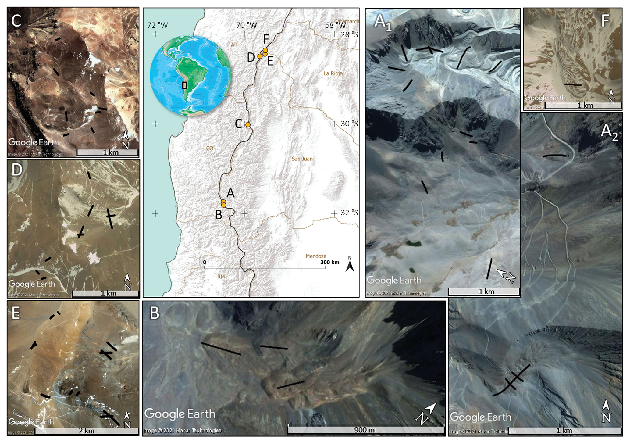
Figure 1 Map of the Central Andes with the study sites A–F (map sources: ESRI, USGS, NOAA) and detailed images for each of the study sites, showing the geophysical lines completed (Map data: © Google Earth 2021).

2 Methods

Our electrical resistivity tomography (ERT) and refraction seismic tomography (RST) surveys followed the well-established methods described in Halla et al. (2021), Mewes et al. (2017), and Mollaret et al. (2019). This includes the conduction of the surveys, data processing with filtering of measured apparent resistivity (ERT), first break picking (RST), data inversion using the software RES2DINV (Aarhus Geosoftware) and REFLEXW (Sandmeier Geophysical Research), and, where applicable, running the four-phase model (Hauck et al., 2011).

We collected ERT data in the field using a Syscal multi-electrode instrument (Iris Instruments) with 48 electrodes. As ERT data acquisition quality often suffers from low signal-to-noise ratios induced by the high contact resistances of galvanically coupled electrodes in dry and coarse-blocky substrates, all measurements were performed in the Wenner configuration to ensure maximum signal strength. The spacing between the electrodes for the individual profiles varied between 1 and 8 m depending on the desired survey geometry and penetration depth. The obtained apparent resistivity data sets were filtered following the procedure described in Mollaret et al. (2019). Data inversion was conducted using the software RES2DINV (Loke, 2020) and typical inversion parameters used for heterogeneous and highly resistive terrain (Hilbich et al., 2009; Mollaret et al., 2019). Inversions with other schemes such as the open-source library pyGIMLi (Rücker et al., 2017) gave comparable results (Mollaret et al., 2020).

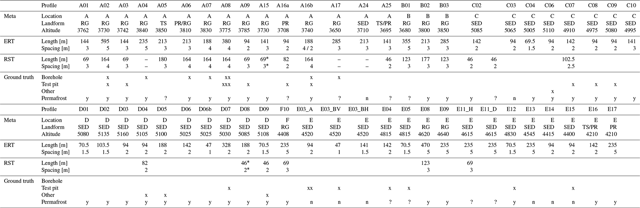
Table 2 Summary of all ERT and RST profiles in all regions, including classification into landform types, availability of ground truthing data, and indication of permafrost presence or absence, when possible. Abbreviations: RG = rock glacier; TS = talus slope; SED = sediment slope (including gelifluction slopes, colluvial slopes, debris-covered bedrock, moraines, landslides). Asterisks (^*) indicate data sets which are available but were not used in this study.

Refraction seismic data were recorded using a Geode system (Geometrics) with 24 geophones and a sledgehammer source. First breaks were picked manually and afterwards inverted within the software REFLEXW (Sandmeier, 2020) to yield tomograms of P wave velocity on co-located lines of specific ERT profiles. The resolution and data quality differ for each profile and method; in general, the resulting root mean square (RMS) errors of the ERT profiles were below 10 % (except for E17 with 22 %) and below 3 ms for the RST inversion (see Appendix, Table B1). See Table 2 for details on the individual profiles.

Regarding quantification of the volumetric ground ice content (ice content), the obtained specific resistivity and P wave velocity distributions can be used as input variables to model estimates of the volumetric phase contents in the pore space (ice, water, air) using the so-called four-phase model (4PM) introduced in Hauck et al. (2011). The 4PM consists of a combination of two basic mixing rules for electrical resistivity (Archie's law; Archie, 1942) and seismic P wave velocities (a modified Wyllie equation; see Timur, 1968), as well as the condition that the volumetric contents of ice, water, air, and rock sum up to 1 for each model cell. Under the assumption of a site-specific porosity distribution, the 4PM estimates the ice, water, and air content for each model cell (see Appendix A for details of the 4PM approach). Wagner et al. (2019) extended the approach to better exploit the complementarity of the independent data sets by jointly inverting these electrical and seismic data sets in order to reduce the model parameter uncertainties. This petrophysical joint inversion (PJI) model yields physically consistent estimates of all four phases, i.e. without the necessity of prescribing porosity. Both model approaches were successfully applied to various permafrost occurrences (Halla et al., 2021; Mollaret et al., 2020; de Pasquale et al., 2020; Pellet et al., 2016; Schneider et al., 2013). However, the PJI still faces convergence problems in the absence of in situ knowledge (Mollaret et al., 2020), and its application to a large number of geologically and geomorphologically different profiles is therefore challenging. Hence, we opted here for the application of the 4PM, which allows consistent ice content modelling for a large number of profiles.

In the 4PM, the largest uncertainties in absolute ground ice content values are due to the absence of reliable porosity information and extreme values of pore water resistivity. The latter are a factor in Archie's law that must be prescribed (Hauck et al., 2011). Halla et al. (2021) established a procedure using ranges of porosity and pore water resistivity values to quantify the uncertainty in absolute volumetric ice content estimates of a rock glacier in the Argentinian Andes. We follow here a similar approach by using three different 4PM runs spanning over the most probable porosity range for the respective landforms, and the resulting minimum and maximum ice content values were used as the uncertainty range in the comparative analysis of all data (see Sect. 4.4.2).

Within this study, we primarily used ERT surveys to detect ground ice occurrences and delineate their vertical extent. As seismic surveys are much more time consuming, they were conducted only at specific ERT profiles to get quantitative ice content estimates at representative locations. As co-located ERT and RST profiles are necessary to provide input data for the 4PM, these model results are only available for 22 profiles (see Table 2). Ice content estimates and ground ice extent were estimated from ERT data alone for all other profiles. We hereby selected so-called zones of interest (ZOIs) within the ERT tomograms (see Etzelmüller et al., 2020), which we consider to be representative of the landforms and permafrost occurrences. Within the respective ZOIs we evaluated resistivity averages and maxima as proxies for ground ice content. Validation data are available for several profiles and ZOIs through drill cores, borehole temperature information, and test pits (see next section).

3 Study sites and data set

Between 2016 and 2019, five extensive geophysical campaigns were completed in three different regions of the Central Andes on both sides of the border between Chile and Argentina. In total, 52 ERT and 24 RST profiles were acquired to characterize permafrost conditions regarding extent, active layer thickness, and ground ice content. All field data were acquired in the austral summer as part of characterizing the periglacial environment. Profile locations were chosen according to the probable presence of frozen ground but also according to easy access and safety. Apart from the fact that some of the considered permafrost landforms had surface disturbances (e.g. access roads or drilling platforms), the context of developing environmental impact assessments for mining projects has no further relevance for the scientific content of this paper. The available infrastructure, however, enabled access to high-altitude permafrost environments and made possible the collection of a large and unique data set, including in situ validation data.

Figure 2 Photographs of typical landforms with survey lines.

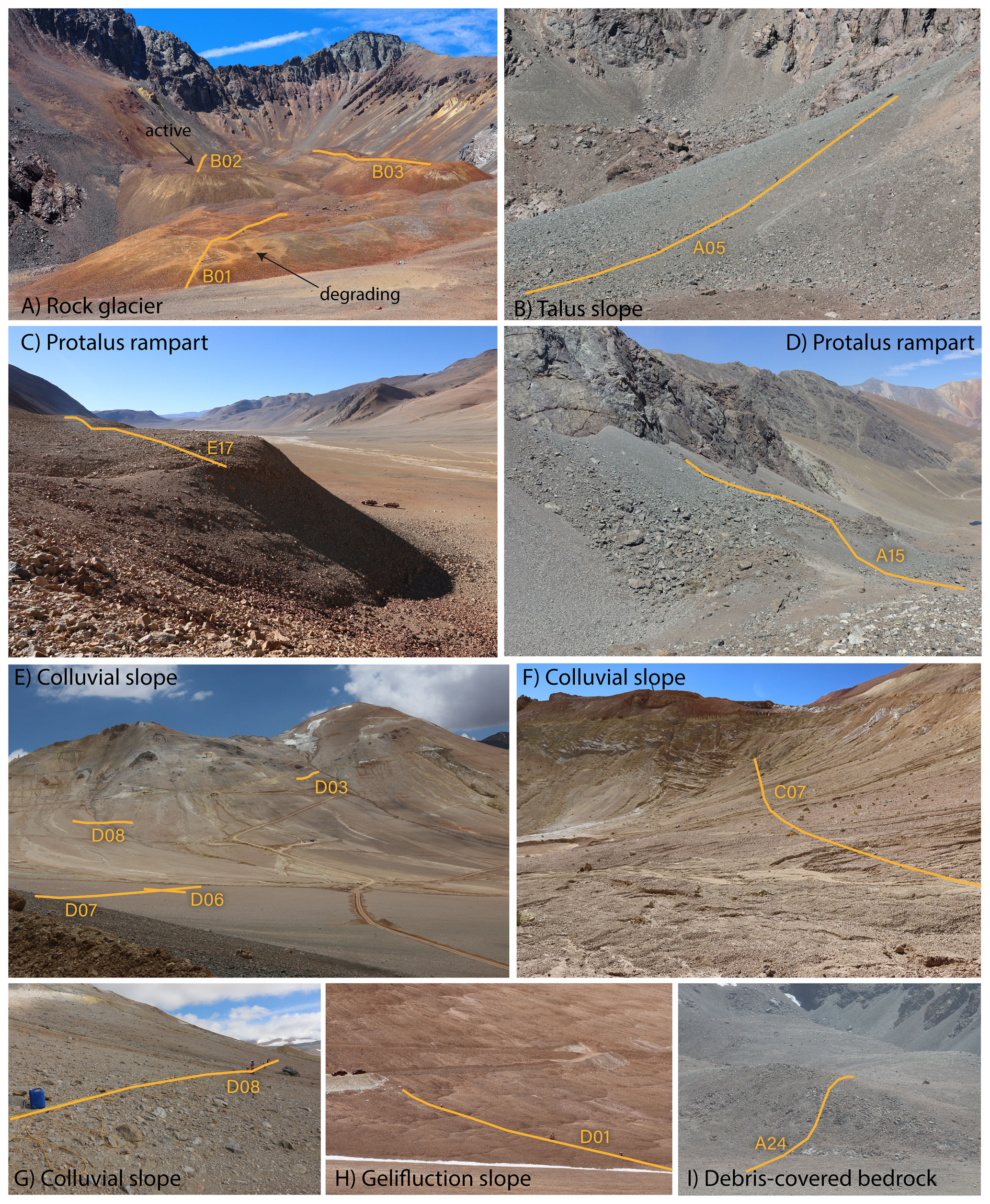
Due to the different locations (see Fig. 1), a large variety of ground conditions ranging from sediment slopes (including gelifluction slopes, colluvial slopes, debris-covered bedrock, moraines, landslides), talus slopes, protalus ramparts (also called protalus rock glaciers or embryonic rock glaciers; see Barsch, 1996; Hedding, 2011), and rock glaciers were covered by geophysical profiles. Table 1 summarizes the main characteristics of the different study sites and geophysical profiles, and Fig. 2 shows some typical examples of the considered landforms with the geophysical profile lines indicated. Many of the rock glaciers in the different investigation areas show initial or advanced signs of degradation (e.g. inactive front slopes, thermokarst depressions), but in the absence of kinematic data for most of the observed rock glaciers a reliable determination of their activity state according to the guidelines of the International Permafrost Association (IPA) action group on rock glacier inventory and kinematics (RGIK, 2020) remains challenging. As the activity of a rock glacier is not directly linked to its ice content, which is the focus of this paper, we avoid any pre-classification of the rock glacier activity here even if geomorphological indications and kinematic data are available in some cases.

In total 22 coinciding ERT and RST profiles were subsequently used for the estimation of the ground ice content and its spatial variability based on the 4PM. The availability of undisturbed core drillings, borehole temperature measurements, and numerous test pits enabled the validation of the methodological approach at 24 of the profile lines (availability of ground truthing data indicated in Table 2).

4 Results

All available data (ERT and RST) have been quality-checked, processed, and interpreted. An overview of data quality (filter statistics, RMS error), and a reference plot with all available ERT and RST tomograms is provided in Appendix B (see Table B1, Figs. B1–B4). In the following, we will present exemplary results of different landform characteristics.

4.1 Rock glaciers and protalus ramparts

4.1.1 General characteristics

In total, we acquired 19 ERT profiles on ice-rich permafrost landforms, including rock glaciers (16 profiles) and protalus ramparts (3 profiles). These are shown in Fig. 3 with the same dimensions and colour scales for all tomograms. We analysed and interpreted all profiles independently in the framework of unpublished internal reports for the respective EIAs (Hauck et al., 2017; Hilbich et al., 2018; Hilbich and Hauck, 2018a, b, 2019); here, we focus on a general and comparative analysis of all profiles as a detailed discussion of each case study is beyond the scope of this paper. The interpretation of the data and specifically the regional assessment is unique and is beyond what the surveys have been used for during the EIAs.

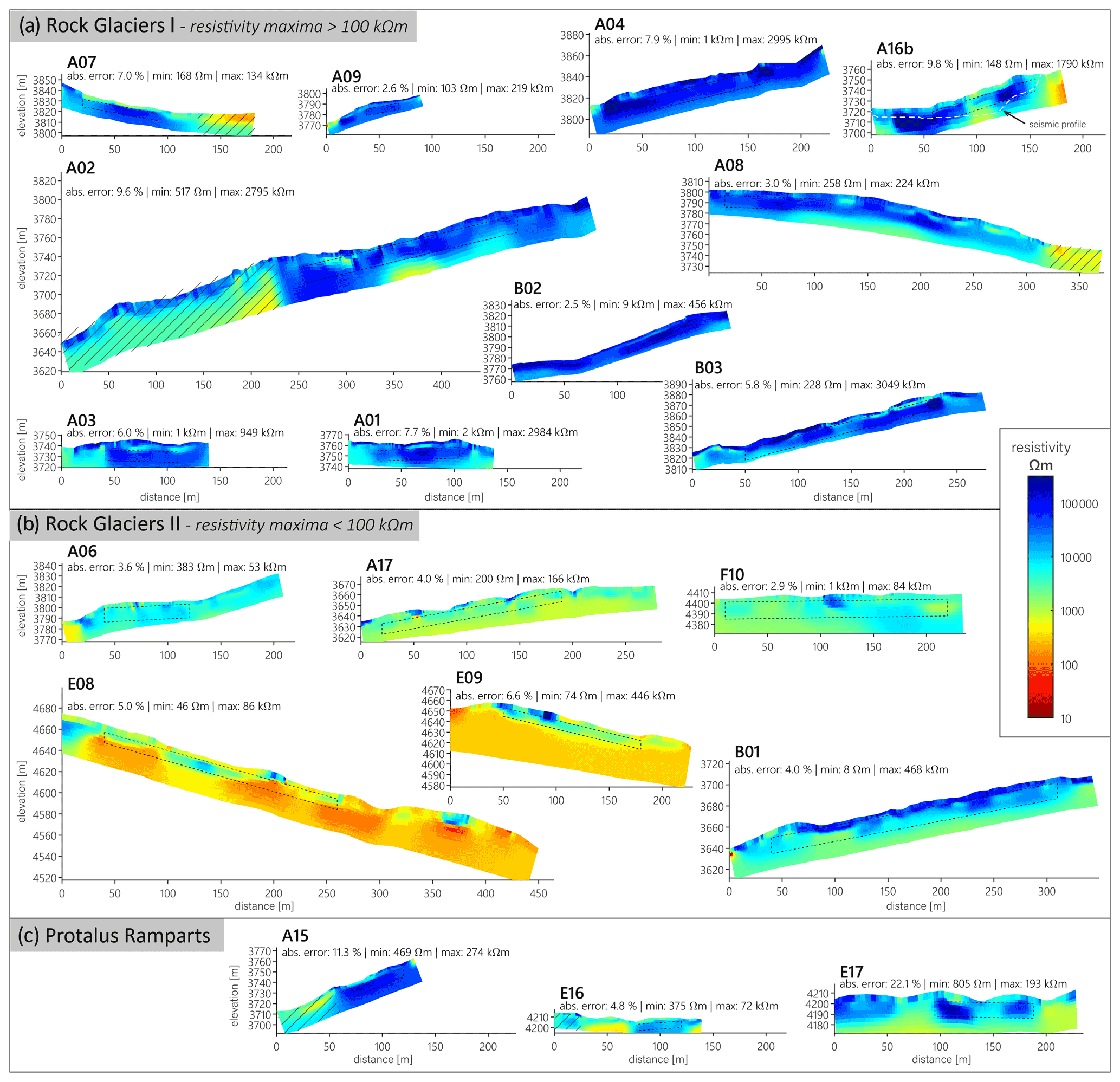
Figure 3 Inverted ERT tomograms for all rock glacier and protalus rampart profiles of the study. Zones of the tomograms not related to a rock glacier or protalus rampart are indicated by diagonal lines. The dashed rectangles mark the so-called zone of interest (ZOI) used for the resistivity averaging and comparison. The data misfit (absolute error in %) is indicated for each profile. The position of the seismic profile shown in Fig. 5 is highlighted in profile A16b.

Among our data, the resistivity of rock glaciers can be split into two groups: rock glaciers with resistivity maxima of the permafrost body below the active layer well above 100 kΩm, some reaching 1 MΩm or more (RG I, Fig. 3a), and rock glaciers with resistivity maxima mostly < 100 kΩm and/or shallower and more patchy resistive zones (RG II, Fig. 3b). Rock glaciers of group RG II often show visible degradation expressions, such as inactive front slopes or thermokarst depressions. Protalus ramparts show similar resistivity values as rock glaciers (Fig. 3c).

Note that rock glaciers with a very coarse-blocky and dry active layer (with air-filled voids) typically can have similarly high resistivity in the active layer as in the ice-rich permafrost layer as both air and massive ice are electrical isolators (e.g. profiles A04, A15). However, at the bottom of the active layer, more fine-grained material typically accumulates, and moisture from snowmelt and seasonal active layer thawing may be retained on top of the impermeable frozen layer, often resulting in a more conductive intermediate layer (e.g. visible in A01, A03, A08, A09; see Fig. 3a).

A high-resistivity zone indicating ice-rich permafrost can usually be observed throughout the entire landform for rock glaciers of group RG I but with varying thicknesses and specific resistivity values. We estimate the thickness of the ice-rich permafrost body of the rock glaciers from the thickness of this high-resistivity zone. As the resolution of geophysical methods generally decreases with depth, the determination of the upper boundary is more reliable than its vertical extent. The resolution of the lower boundary depends on several factors:

• a.

  survey geometry, defining the spatial resolution and the depth of investigation,

• b.

  the depth of the lower boundary in relation to the investigation depth (the shallower the boundary, the better its resolution), and

• c.

  the resistivity contrast between the ice-rich permafrost layer and underlying layer (e.g. bedrock: the higher the contrast, the better the resolution).

We therefore use the onset of a decreasing resistivity gradient (below the maximum) as a conservative indicator for the lower limit of ice-rich permafrost.

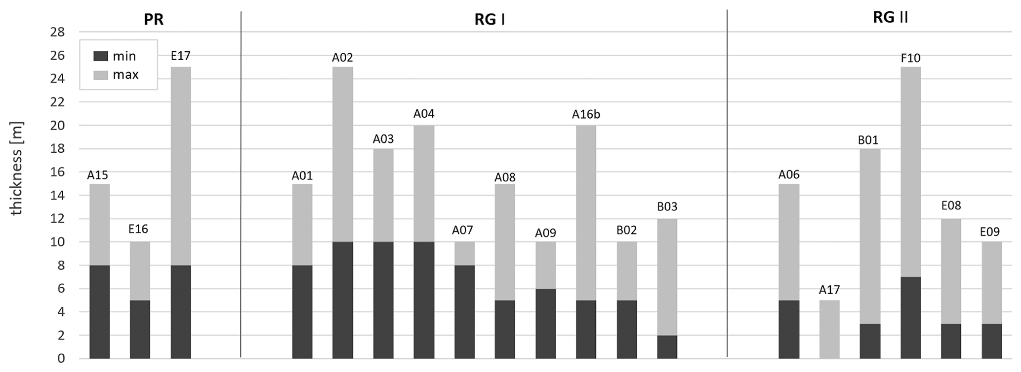
Figure 4 Overview of minimum and maximum thickness of ice-rich permafrost in all protalus ramparts (PRs) and rock glaciers (RGs) of groups I and II, determined from the high-resistive zone in the ERT tomograms. Profile A17 is from a relict rock glacier with little probability for ground ice.

The investigation depth was sufficient to identify the bottom of the ice-rich permafrost layer for most rock glacier profiles. Due to the spatial heterogeneity within the observed profiles, the thickness of the ice-rich permafrost layer cannot reliably be determined everywhere along the profile. Figure 4 indicates the ERT-based minimum and maximum thickness of the ice-rich layer in all ice-rich permafrost profiles (i.e. rock glaciers and protalus ramparts). Note that the minimum thickness refers to the ice-rich zones within the tomograms and that most profiles also contain zones without permafrost or ice-rich layers. The determined thicknesses mainly range between a few metres and 25 m, which they do not exceed, for all considered landforms. No clear difference is observed for the different categories, nor was one expected.

As an overall observation, it can be noted that data quality is often worse on the coarse-blocky parts of the rock glaciers because of challenging conditions for sufficient galvanic coupling at the surface (Hilbich et al., 2009; Mollaret et al., 2019) than for the generally more fine-grained surface material and lower resistivity of rock glaciers with advanced degradation (RG II). This clearly affected the data quality in the first half of profile E17 (22 % data error; see Figure 3c) but had no severe impact on most other profiles. A few more profiles with insufficient data quality exist but were not considered for this study.

4.1.2 Example data set: rock glacier profile A16B

As an example, Fig. 5 shows the geophysical results for profile A16B, which crosses two neighbouring rock glacier lobes, with a borehole drilled in one of the lobes marked by the vertical black line. The active layer was largely removed through the construction of the drilling platform. Maximum resistivity values of up to 1 MΩm are observed in two distinct anomalies corresponding to the two different lobes and indicate high ground ice content occurrences of 5–18 m thickness, which is confirmed by the drilling results (see Figs. 5a, 6, Table 3).

The corresponding seismic results (Fig. 5b) confirm ice-rich permafrost with P wave velocities of 3000–4000 m s⁻¹ within the zone of the high resistivity anomalies. Below this zone, P wave velocities of up to 6000 m s⁻¹ indicate the bedrock at around 20 m depth. The profile clearly illustrates coinciding characteristic resistivity and velocity values for pure ice (ρ>1 MΩm and v_p=3500 m s⁻¹) and bedrock (ρ∼1 kΩm and v_p=6000 m s⁻¹; see Hauck et al., 2011).

Based on the co-located ERT and seismic profiles, the volumetric fractions of the four phases, rock, ice, water, and air, have been modelled using the 4PM (see Sect. 2). Figure 5c shows the modelled ice content for profile A16B, with two anomalies of > 60 % ground ice content, which is in good agreement with the previous interpretation (Fig. 5a, b) and the results from the borehole stratigraphy. The thaw depth is around 3–5 m in both lobes (except for the disturbed area of the drilling platform).

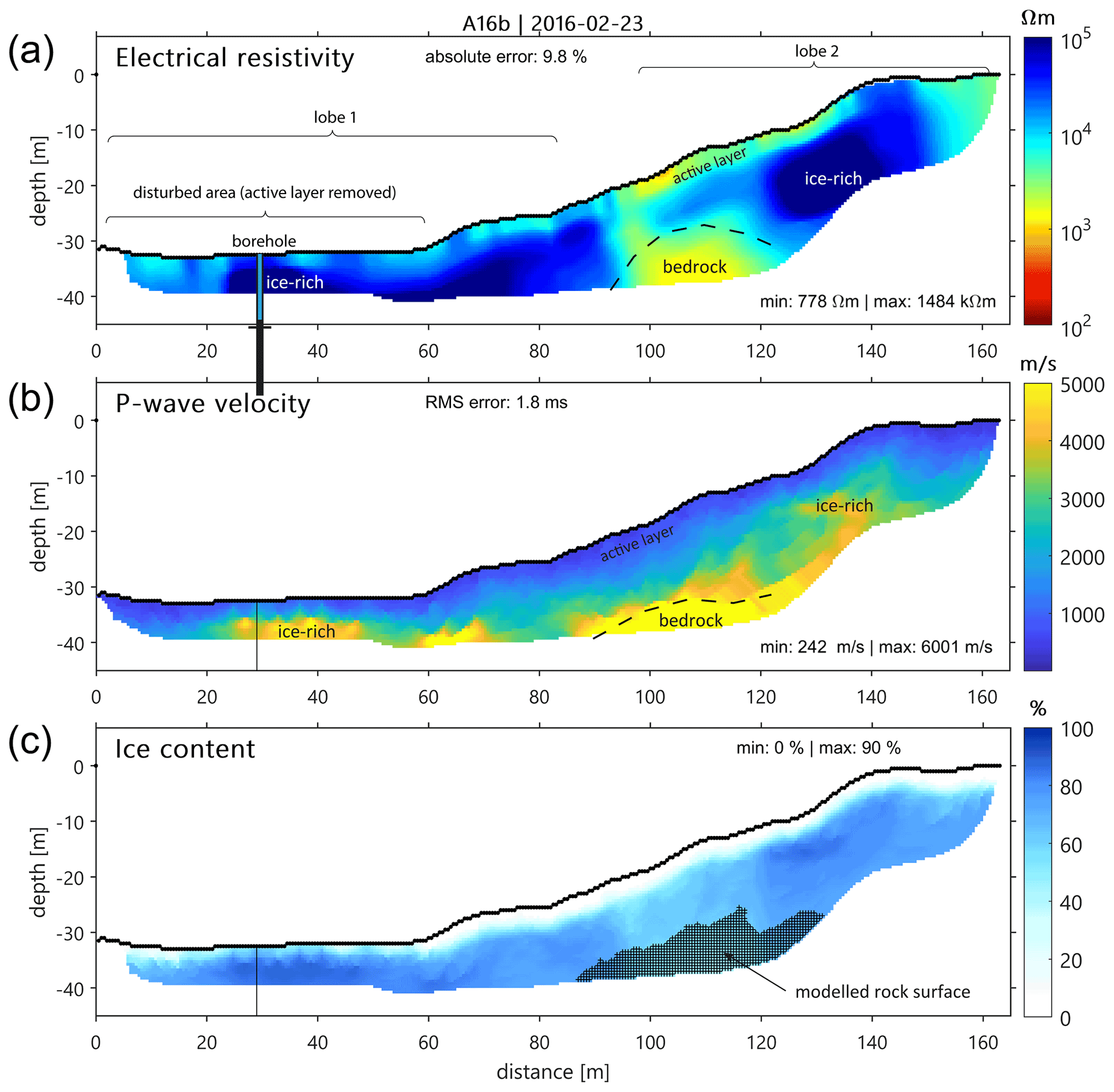
Figure 5 Geophysical results of profile A16B (rock glacier): (a) section of the ERT profile covered by the RST profile (see Fig. 3a for full profile), (b) RST profile, and (c) volumetric ice content modelled by the 4PM. The borehole position is highlighted, with the light blue part indicating the frozen part. Minimum and maximum values are indicated for all three tomograms, as well as the data misfit of both inversion models. The cross-hatched zone marks the area detected as bedrock in the 4PM. Labels denote the interpretation.

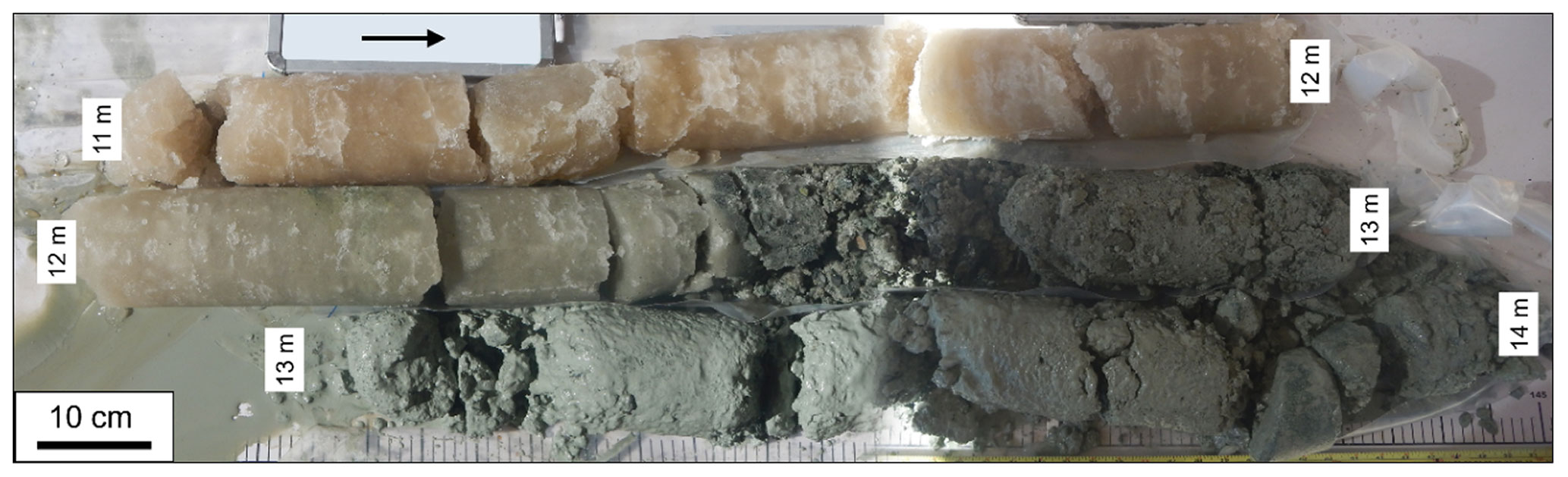
Figure 6 Example of a frozen core extracted from a rock glacier at 11–14 m depth (ERT profile A16b). The upper half of the core run shows massive ground ice and the lower half frozen gravel and sand with a very low ground ice content.

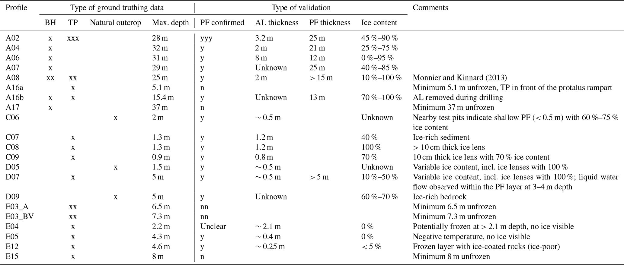
Table 3 Overview of available ground truthing data with the most important permafrost-relevant information. Abbreviations: BH = borehole; TP = test pit; PF = permafrost; AL = active layer. The presence of one or more boreholes or test pits is indicated with one or more x's; similarly one or more y's indicate if permafrost was confirmed or n's for unconfirmed. The ice content range represents the observed minimum and maximum values throughout the entire depth column.

4.2 Talus slopes

4.2.1 General characteristics

ERT profiles were collected on three talus slopes, and all of them show a similar resistivity pattern: a layer of increased resistivity (∼ 10 kΩm) within the talus material having a bulk resistivity of only a few thousand ohm metres (Fig. 7). The resistive layer is located at depths > 3 m, i.e. below a potential active layer, and has a maximum thickness of 10 m for the four measured profiles. The resistivity values are sufficiently high to support the hypothesis of frozen conditions within the talus slope (Hauck and Kneisel, 2008) even if the expected ground ice content is low. The resistive zone could also be explained by purely air-filled voids within the porous coarse-blocky substrate, similar to the resistive anomalies visible directly at the surface in most profiles. This ambiguity can, in general, be addressed using coinciding seismic profiles (available for A05, A16a, and A25). Exemplary cases are shown in Sect. 4.2.2. Unfortunately, no ground truthing information is available for any of the talus slopes.

4.2.2 Example data set: talus slope profile A05

Profile A05 is a longitudinal profile within a talus slope, located on an east-facing slope in the western part of a valley with numerous rock glaciers on its south- and west-facing slopes. The ERT results in Fig. 8a show comparatively low resistivity of < 10 kΩm in most parts of the profile, indicating no or very small ground ice content. A localized anomaly with higher resistivity (ρ≥10 kΩm) exists between 80 and 140 m horizontal distance and suggests a small possibility for potential ground ice at approximately 5–12 m depth. Seismic velocities of v_p < 1500 m s⁻¹ in the same region point to loose blocks and debris with air-filled voids (Fig. 8b) rather than a layer with massive ground ice, except at greater depths (∼ 25 m) where higher P wave velocities (v_p ∼ 2000–3000 m s⁻¹) and coinciding low resistivity values (ρ < 5 kΩm) strongly indicate bedrock. No ground truthing data are available for this profile. The anomaly with slightly larger resistivity values around 10 kΩm between distances of 80 and 140 m could indicate frozen conditions but with volumetric ice contents, which are too small to be detected by our seismic survey set-up. Consequently, the 4PM-estimated ice content is close to zero within the whole model domain (Fig. 8c).

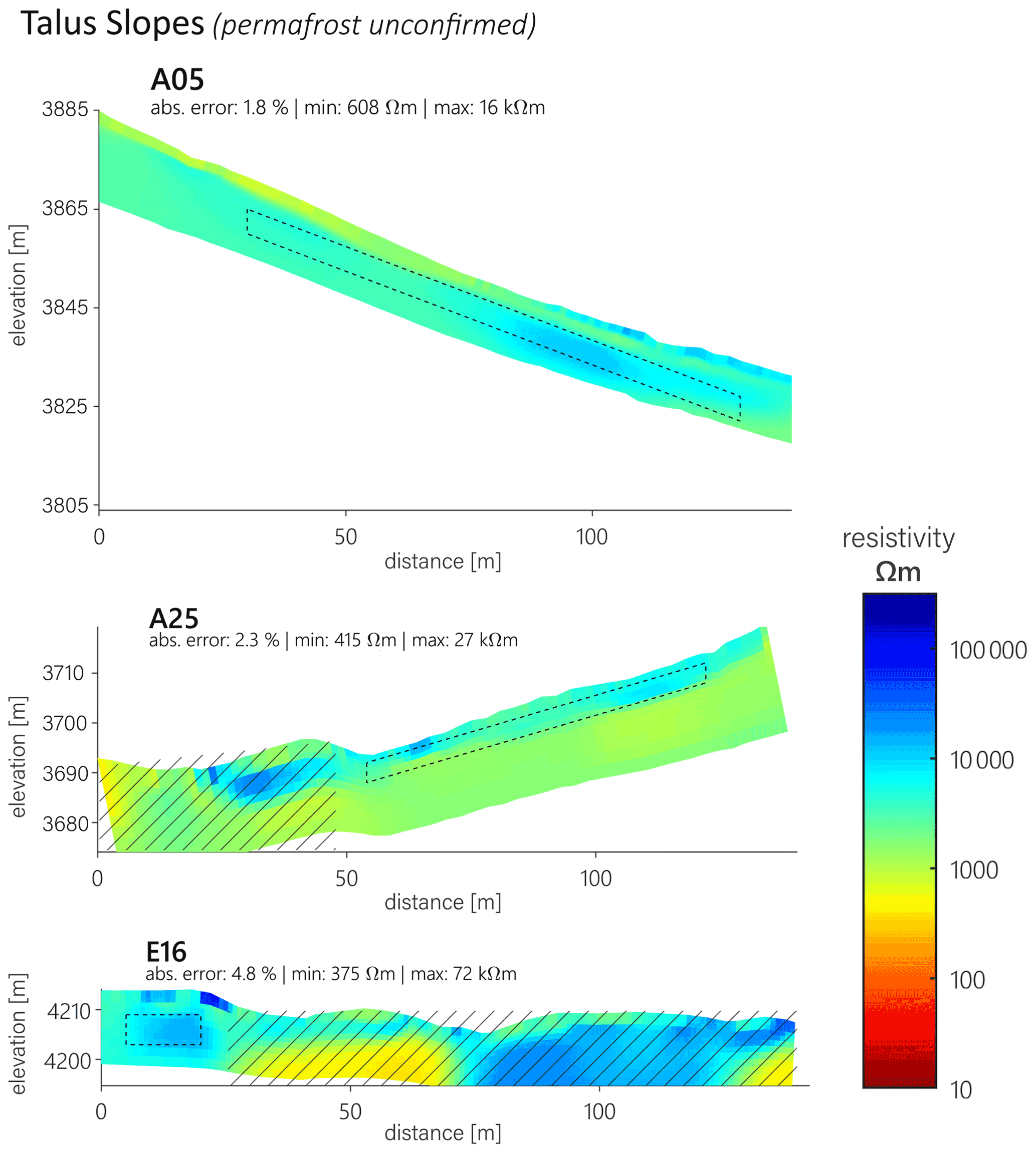
Figure 7 Inverted ERT tomograms for all talus slope profiles of the study. Zones of the tomograms not related to the talus slope are indicated by diagonal lines. The dashed rectangles mark the so-called zone of interest (ZOI) used for the resistivity averaging and comparison. The data misfit (absolute error in %) is indicated for each profile.

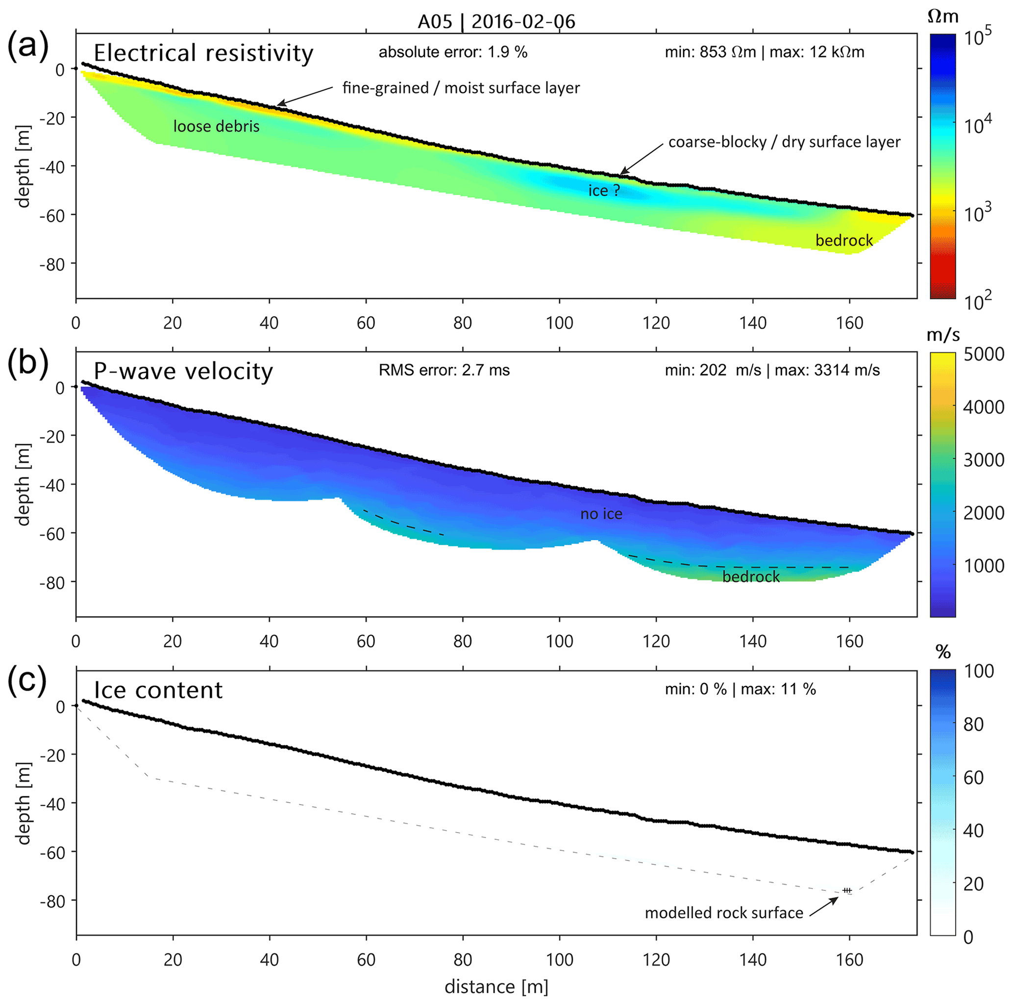
Figure 8 Geophysical results of profile A05 (talus slope): (a) ERT profile, (b) RST profile, and (c) volumetric ice content modelled by the 4PM. Minimum and maximum values are indicated for all three tomograms, as well as the data misfit of both inversion models. The cross-hatched zone marks the area detected as bedrock in the 4PM. Labels denote the interpretation.

4.3 Sediment slopes

4.3.1 General characteristics

In addition to the 22 profiles on pebbly and coarse-blocky substrates of rock glaciers, protalus ramparts, and talus slopes, 30 additional ERT profiles were measured on more fine-grained sedimentary substrate, including colluvial slopes (17 profiles), gelifluction slopes (4 profiles), and weathered bedrock covered with a shallow debris layer (9 profiles; see Appendix, Fig. B2). Some of these ERT profiles on sediment slopes do not contain permafrost (e.g. E03, E13, E14, E15; see Table 2). However, all profiles on sediment slopes show significantly lower resistivity values (mostly well below 1 kΩm) compared to rock glaciers, protalus ramparts, and talus slopes (see Appendix, Fig. B1), including those where ground ice was confirmed by test pits or outcrops (e.g. D07, D09, C06, C08). The reduced resistivity values are a result of the fine-grained and partly humid substrate and/or the weathered bedrock, as well as the generally lower volumetric ice content in sediment slopes in the form of interstitial ice (i.e. ≪ 50 %, except for excess ice in mostly thin ice lenses).

In addition, many of these profiles contain prominent conductive layers of < 100 Ωm (Appendix, Fig. B2). We speculate that this is mainly caused by (a) conductive sediments stemming from eroded hydrothermally altered bedrock, which was transported downslope (in the case of colluvial slopes), (b) the altered/conductive bedrock itself, or partly also (c) liquid (supercooled) water due to freezing point depression by increased ion content related to hydrothermal alteration (Hauck et al., 2017; Hilbich and Hauck, 2018a). Significant water flow was for example observed above an ice-rich layer in a 4–5 m deep test pit close to profile D07 and below a frozen layer in profile C08 (see Appendix, Fig. B2a). It is important to note that these conductive layers are, with high probability, features strongly amplified by the inversion process caused by preferential current flow through conductive layers, which strongly biases the inversion result towards this conductive layer. Various synthetic modelling studies (e.g. Hilbich et al., 2009; Mewes et al., 2017) have shown that the real thickness of such conductive layers may be more than an order of magnitude smaller than illustrated in the resulting tomograms. In this case, the resistivity of layers below will be biased towards lower values. Ice contents may well be higher than expected from the inverted values, and the depth of the deeper layers could also be strongly overestimated.

The detection of permafrost occurrences is further complicated by the often thin or patchy ice lenses which cannot be detected with confidence because of the trade-off in the electrode spacing between reasonably large investigation depth/profile length and the resulting reduced spatial resolution capacity. A reliable interpretation of these tomograms is therefore not straightforward, but experience from the synthetic modelling studies mentioned above and comparison with ground truthing information allow resistive anomalies caused by small ice lenses to be identified even if absolute resistivity values are lower than commonly known to indicate frozen conditions. Similar cases are known from the European Alps, where the combination of low-resistive geologic host material, increased water content, and temperatures close to the freezing point leads to similarly low permafrost resistivity (Hilbich et al., 2008; Mollaret et al., 2019; Noetzli et al., 2019).

Permafrost was clearly detected in profiles C07, D04, D05, and D09, where a prominent resistive layer (> 10 kΩm) is observed. Similar values but within much smaller and thinner anomalies were found in profiles D06, D07, and D08. Test pits and natural outcrops within incised channels confirm the presence of permafrost for profiles D04–D07 and D09 (see Appendix, Fig. B2).

4.3.2 Example data set: colluvial slope profile D04

Figure 9 shows the results of profile D04 located within an east-facing slope and consisting mainly of fine-grained colluvial sediments, cut by incised channels which are active during snowmelt (see Fig. 2e). The slope shows a slightly convex form, indicating the potential for ice-rich conditions. The ERT tomogram in Fig. 9a shows a high-resistive layer with values up to 10 kΩm indicating ice-rich permafrost between approximately 2 and 8 m depth, with a maximum around 3 m depth. Maximum resistivity values are similar to the maximum values in profile D09, where ground truthing from a test pit confirmed ice contents ≥ 50 %. We therefore expect significant ice-rich layer(s) in this profile with a possibly supersaturated zone around the resistivity maximum. The presence of ice-rich sediments is further confirmed by a natural outcrop formed by an incised channel close to profile D04, which exposed ice-rich and partly supersaturated sediments at about 1 m depth (thickness of this layer unknown).

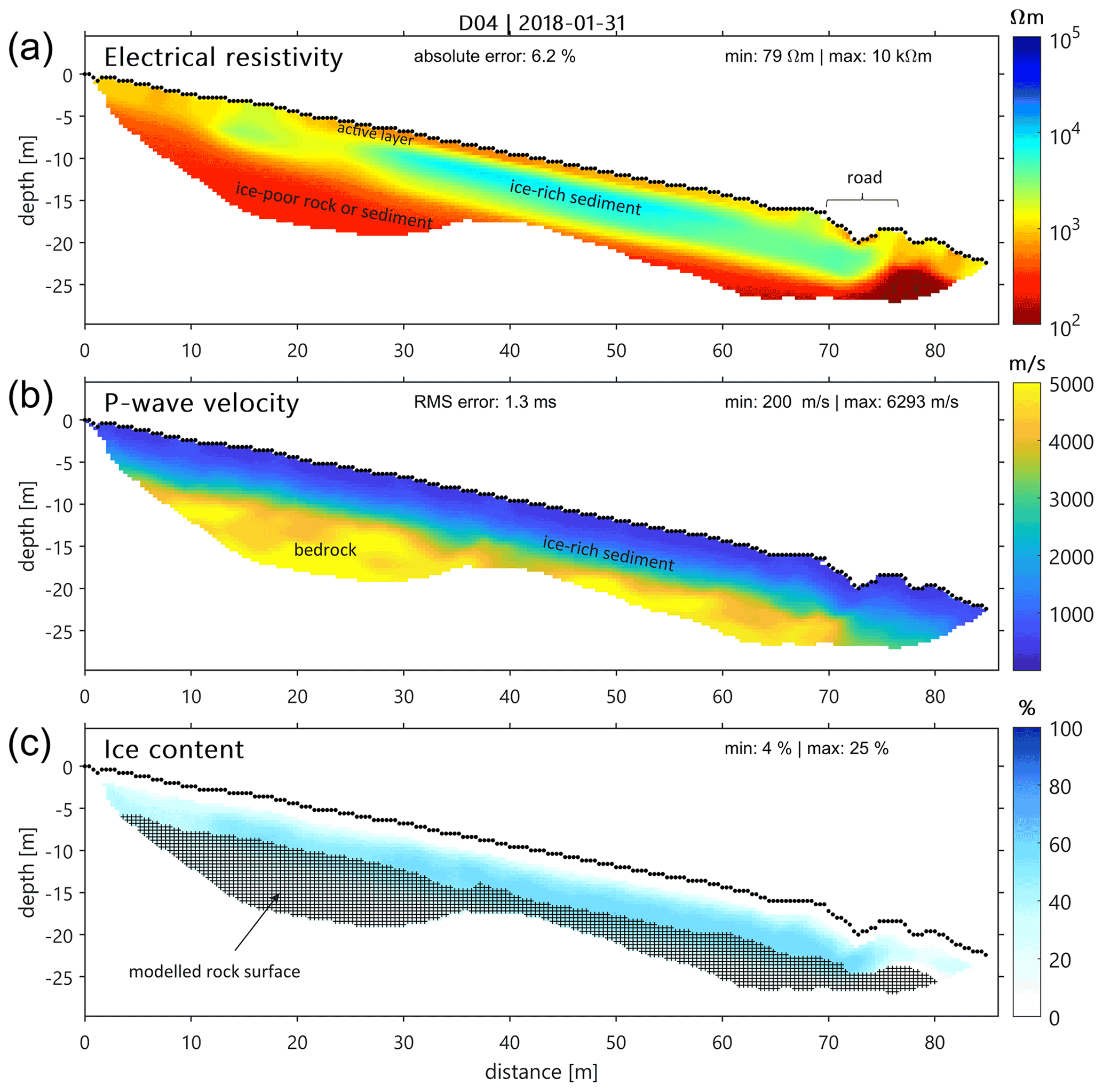
Figure 9 Geophysical results of profile D04 (colluvial sediments): (a) section of the ERT profile covered by the RST profile (see Appendix, Fig. B2 for full profile), (b) RST profile, and (c) volumetric ice content modelled by the 4PM. Minimum and maximum values are indicated for all three tomograms, as well as the data misfit of both inversion models. The cross-hatched zone marks the area detected as bedrock in the 4PM. Labels denote the interpretation.

Below this ice-rich layer, resistivity values < 500 Ωm indicate ice-poor conditions, while a reliable differentiation between sediment or bedrock is not possible without further information. Seismic P wave velocities increase to > 5000 m s⁻¹ at ∼ 10 m depth and indicate a transition to more competent frozen rock at this depth (Fig. 9b).

Figure 9c shows the modelled ground ice content with maximum values around 60 %, which confirms the expected high ground ice contents in this profile. The highest values are observed between 30 and 70 m horizontal distance with decreasing values in upslope direction (40 %–50 %) and an abrupt change to values < 30 % near the road in the lower part of the profile.

4.4 Joint analysis

4.4.1 Mean resistivity and P wave velocity

Comparing mean resistivity and P wave velocities of the various profiles is a delicate task due to their dependence on (potentially very different) local geologic conditions, which may give rise to substrate-dependent resistivity–velocity variations that may be misinterpreted as differences in ground ice content. Uncertainties due to different measurement configurations and inversion errors may further impact a joint comparison. On the other hand, the dependence of resistivity and P wave velocity on ice content is very strong, and its signal should be clearly detectable in the large and comparatively homogeneous data set presented in this study.

For a joint analysis of the representativeness of the measured geophysical parameters for the considered landforms, we selected all profiles where the presence of permafrost (a) has been identified or (b) is considered possible but not confirmed (e.g. in talus slopes; see Table 2). We used the ZOI defined above to select a rectangular zone either within the presumed permafrost occurrence or within the zone most probable for permafrost in the case of ambiguous interpretation in order to base our analysis on a representative zone for the confirmed (or unconfirmed but possible) permafrost occurrence within the respective landform with minimal bias from potential inversion artefacts. Thus, the ZOIs of different profiles are different in terms of sizes and relative positions.

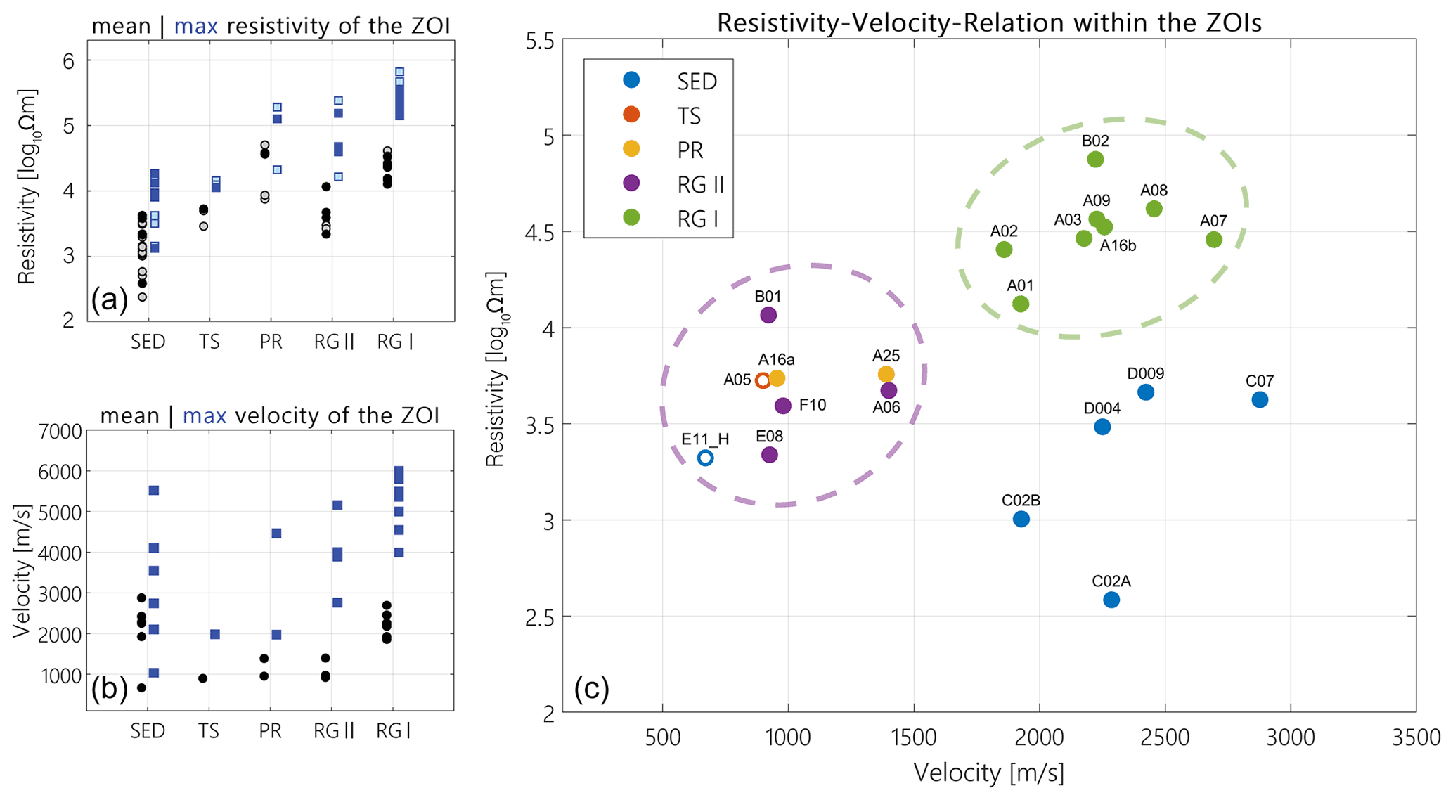
Figure 10 Landform-specific distribution of mean (black) and maximum (blue) values of inverted (a) resistivity and (b) velocity within the ZOIs of the respective electrical resistivity and refraction seismic tomograms. (c) Scatter plot of mean resistivity and velocity for all co-located ERT and RST profiles, classified after landforms. Unfilled symbols in (a) denote ERT profiles without co-located RST profiles. Unfilled symbols in (c) denote ZOIs with only possible permafrost occurrence. Abbreviations: SED = sediment slope (including debris-covered bedrock, colluvial slopes, gelifluction slopes, etc.); TS = talus slope; RG = rock glacier (groups I and II described in Sect. 4.1.1).

Mean and maximum resistivity and velocity values within the ZOIs were then extracted, and they clearly show different resistivity and velocity regimes for different landforms and substrates (see Fig. 10a, b). Figure 10c analyses the relationship between mean specific resistivity and P wave velocity within the ZOI of co-located ERT and seismic profiles and reveals a landform-specific clustering of resistivity–velocity pairs. Hereby, the resistivity–velocity pairs of rock glaciers cluster in two parts (green and purple in Fig. 10c). The purple cluster (lower resistivity and P wave velocity) is consistent with the rock glaciers of group RG II (see Sect. 4.1.1), showing more visible signs of advanced degradation and lower ground ice contents compared to the ones in the green cluster (RG I). Similarly, lower velocity mean values are present for protalus ramparts (PRs) and talus slopes (TSs), with the exception that TSs show lower maximum resistivity values than PRs and RG II probably due to their lower ground ice contents. While the two rock glacier groups clearly differ in their mean resistivity and velocity values, their maximum values overlap probably because most degrading rock glaciers still contain ice-rich zones with similar values as in intact rock glaciers (Fig. 10a, b). Sediment slopes (often reaching bedrock at shallow depths) have clearly differing characteristics from coarse-blocky sites, which is attributed to their lower porosity (higher velocity) and lower ground ice content (lower resistivity). Note, however, that Fig. 10c only provides an incomplete picture biased towards ice-rich landforms as seismic surveys have mainly been conducted on ERT profiles indicating ice-rich permafrost (see Table 2).

A striking pattern in Fig. 10c, with clustered and high resistivity for intermediate velocities (RG I), as well as low–intermediate resistivity for similarly high or even higher P wave velocities (sediment slope: SED), is apparent. This pattern was noted by Hauck et al. (2007) in geophysical surveys on several permafrost landforms in the South Shetland Islands/Maritime Antarctica. Rock glaciers with massive ice cause maximum resistivity but P wave velocities around 3500 m s⁻¹, close to the literature value for ice. Sites with v_p>4000 m s⁻¹ usually indicate the presence of (unfrozen or frozen) bedrock, coinciding with lower resistivity due to the lower ice content. Mean seismic velocities in Fig. 10b are all < 3000 m s⁻¹, which is certainly influenced by the limited investigation depth on some rock glaciers (bedrock not reached) but which also represent the generally lower P wave velocities of hydrothermally altered bedrock in some cases.

The systematic pattern observed in Fig. 10 with a high consistency in the resistivity values over so many different surveys justifies the applicability of the geophysical approach to characterize different permafrost landforms even in the absence of ground truthing. The seismic results further support and confirm the interpretation of the ERT data but with a reduced overall representativeness due to a biased profile selection, fewer profiles, and smaller profile dimension.

4.4.2 Volumetric ground ice contents

Similarly to Fig. 4 (Sect. 4.1.1), Fig. 11a shows the estimated minimum (dark grey) and maximum (light grey) thicknesses of the ground ice layer for all profiles where permafrost is (a) confirmed or probable (indicated by blue frames) or (b) unconfirmed and uncertain but possible. The permafrost base for non-rock-glacier sites could not always be detected; in these cases the base of the surficial ice-rich layer was determined and is plotted instead. It is clear that ice-rich layers in sediments are much thinner than in coarse-blocky substrates. Further, most ice-rich layers within our study are thinner than 25 m, including all rock glacier profiles. Quantitative model results for volumetric ice content (as presented exemplarily above) are available for a total of 21 profiles with co-located ERT and seismic surveys, including 12 rock glaciers, 2 protalus ramparts, 1 talus slope, and 6 sediment slopes. The RST data of B03 were excluded from further analysis due to ambiguous artefacts in the tomogram. Figure 11b shows the modelled mean (dark grey) and maximum (light grey) volumetric ground ice contents within the defined ZOIs for all these profiles. The error bars give the uncertainty resulting from different 4PM runs spanning over the most probable porosity range for the respective landforms (SED: 30 %–45 %–60 %; TS: 40 %–50 %–60 %; RG: 40 %–60 %–80 %). The results indicate that maximum ice contents within the considered ZOIs are 51 %–56 % (±20 %), highest for rock glaciers of group RG I, and between 25 % and 49 % (±20 %) for all other profiles. Note that anomalies with even higher ice contents can be present but cannot explicitly be delineated if their size is smaller than detectable by the measurement configuration. More representative for the landform scale is, however, the mean ground ice content within the considered ZOIs, which is of similar magnitude for most considered profiles (11 %–40 %) and shows that the ice content in the ice-rich layers of sediment slopes can be comparable to those of rock glaciers even if the overall dimension of the ice-rich layer is very different.

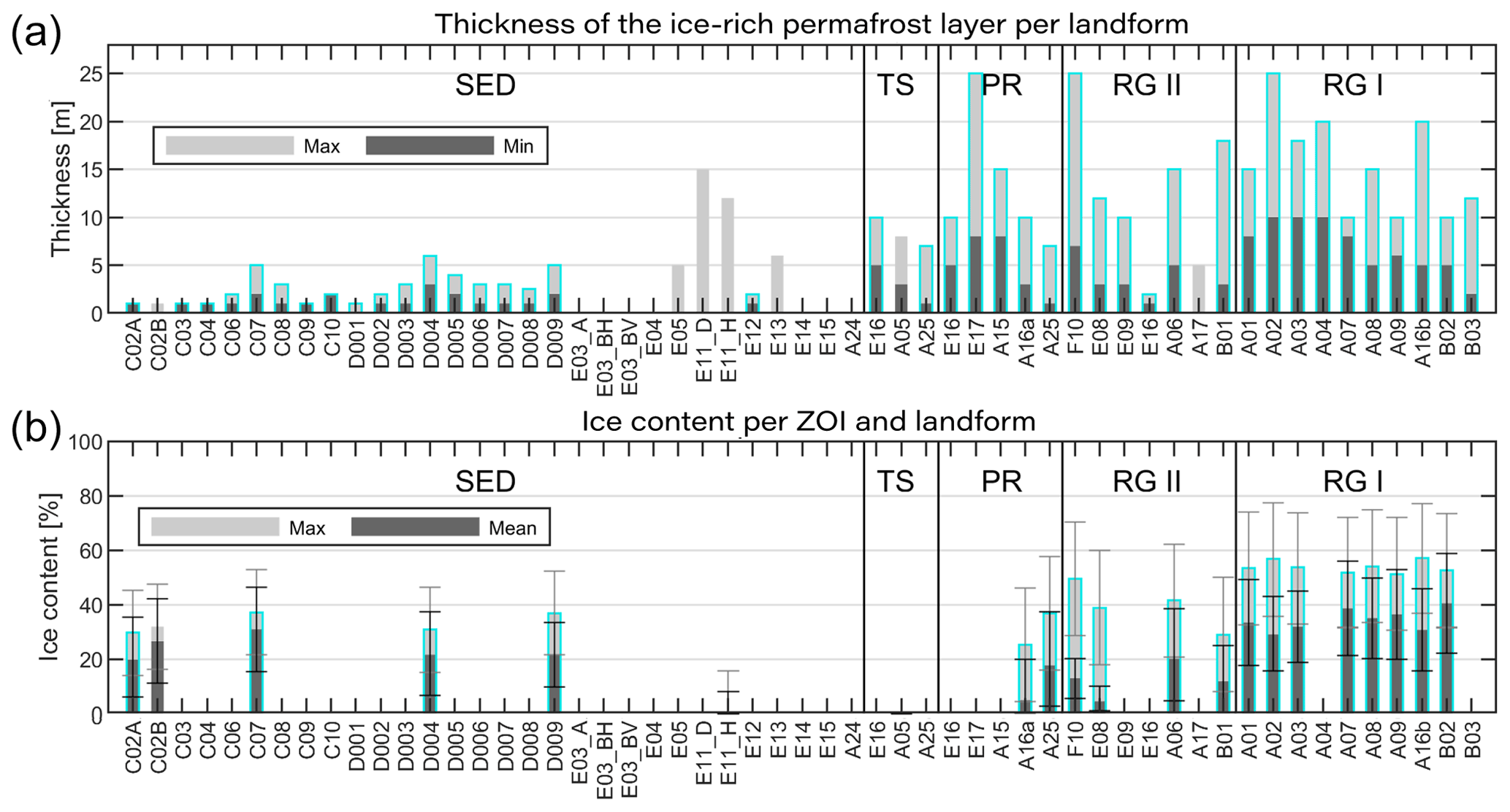
Figure 11 Landform-specific distribution of (a) minimum and maximum thickness of the ground ice layer and (b) the mean and maximum volumetric ground ice content within the ZOIs defined before, as derived from the 4PM. The bars and error bars in (b) are based on landform-specific porosity ranges indicated in the text. Abbreviations: SED = sediment slope (including debris-covered bedrock, colluvial slopes, gelifluction slopes, etc.); TS = talus slope; PR = protalus rampart; RG = rock glacier. Profiles with confirmed or probable permafrost occurrence are highlighted in light blue, while the other values are only based on zones with possible permafrost occurrence.

5 Discussion

The uncertainty of the ice content estimation presented above depends first of all on the standard uncertainties of the geophysical data such as measurement data quality, resolution capacity, investigation depth, potential inversion artefacts, and representativeness of the geophysical profile for the whole landform. In addition, the uncertainties of the 4PM approach (rock–ice ambiguity, porosity range, Archie parameter, and estimate of rock P wave velocity) have to be taken into account. In the context of mountain permafrost studies, 4PM-related uncertainties have already been addressed by Mewes et al. (2017) and Halla et al. (2021). In this study, we make additional use of the opportunity to compare our estimates with available ground truthing information, wherever possible, which when used as calibration reduces the uncertainty considerably. However, a large uncertainty remains regarding the representativeness of the individual profiles for a given landform. Depending on the local geomorphological setting, ground ice contents can vary strongly, especially in the case of very large landforms (e.g. Halla et al., 2021).

5.1 Comparison of results with ground truthing information

Since permafrost is thermally and temporally defined (Muller, 1943) and can be present in different substrates under various porosity and saturation conditions, it can exhibit a wide range of possible values in the geophysical parameters. Attribution of absolute electrical resistivity and P wave velocity values to permafrost presence and specific ice contents can therefore be ambiguous without additional information. Further, the inverted geophysical parameters within a tomogram are influenced by the resolution capacity of the survey geometry in relation to the observed structure, the data quality, and the material contrasts, which may all lead to inversion artefacts (Day-Lewis et al., 2005; Hilbich et al., 2009; Mewes et al., 2017). Small-scale anomalies and thin ice layers may not become visible in the comparatively coarse survey geometries utilized in the majority of the profiles of our study. Therefore, we used ground truth data from the various field sites to validate the geophysical data. Table 3 gives an overview of the different types of available ground truthing data (boreholes, test pits, natural outcrops), the respective depth range covered, and the type of validation provided by the different data.

In general, the interpretation of the tomograms (regarding presence/absence of ice-rich permafrost; see profiles highlighted in blue in Fig. 11a), as well as the overall dimension of the active layer thickness (see ERT tomograms in Appendix, Figs. B1, B2), is confirmed by the ground truthing data, thus enabling the spatial analysis of ground ice occurrence and its quantification.

For some rock glaciers (A02, A06, A07, A08, A16b), borehole-derived ice content values (representing minimum and maximum values observed throughout the borehole) can be compared to 4PM-derived minimum and maximum ice contents within the pre-defined ZOIs (Fig. 12). As thin ice-rich layers can be resolved by direct observations from boreholes or test pits but not necessarily by the relatively coarse survey geometries of the geophysical profiles, maximum ice content values observed in the drill cores are generally higher. In addition, the 4PM cannot model super-saturated conditions (i.e. ice contents exceeding the assumed porosity), which further implies a bias towards underestimated maximum ice contents for the applied porosity ranges (see Sect. 4.2.2). It is therefore not surprising that the borehole-derived ice contents are mostly higher than the 4PM-derived values. Where quantitative ground truthing information is available, the 4PM can be calibrated by minimizing the difference between the estimate and the ground truth, resulting in more consistent ice content values, as illustrated exemplarily in Fig. 13 for a profile with intermediate ice content (A02) and one with high ice content (A16b). Figure 13 further shows that the porosity models of 60 % or 80 % lead to more realistic ice content values than the lower-bound porosity model of 40 %. However, borehole validation provides highly valuable information on the point scale, but a direct comparison of borehole- and 4PM-derived ground ice contents remains challenging due to the different resolution capacities, dimensions (1-D vs. 2-D) and 4PM-related limitations. In the absence of such calibration data, geophysical ice content estimates of ice-rich permafrost layers may be underestimated (as a consequence of underestimated porosity ranges) and rather represent lower-bound estimates. This bias is, however, also a direct consequence of the spatially averaging ZOIs, which also include zones with higher spatial variability and therefore smaller ice contents. On the contrary, boreholes represent single-point information and are usually placed where the maximum ground ice content is assumed.

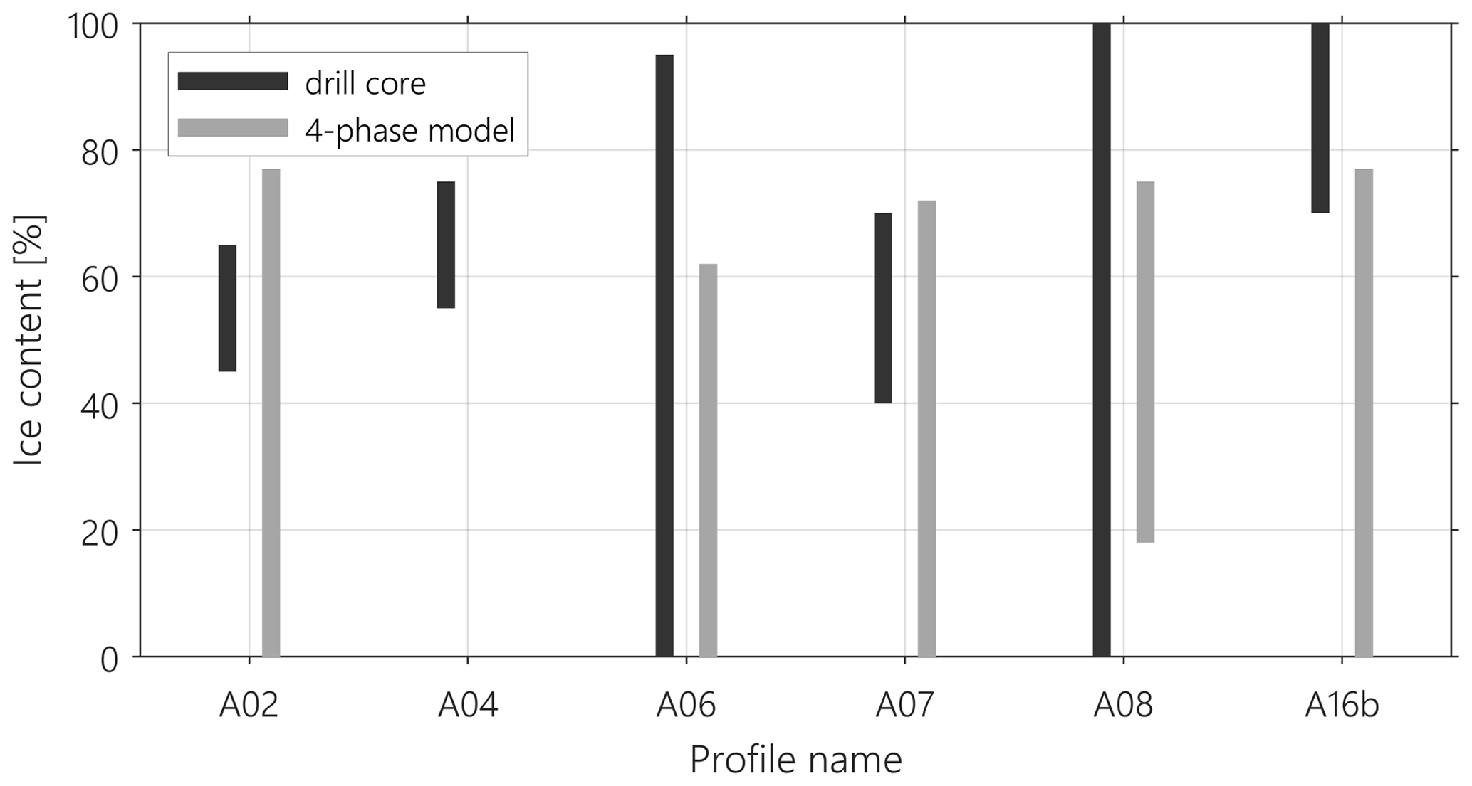
Figure 12 Comparison of borehole-derived with 4PM-derived minimum and maximum ice contents within the pre-defined ZOIs. Here, only borehole values for the depth range covered by the ZOIs are considered.

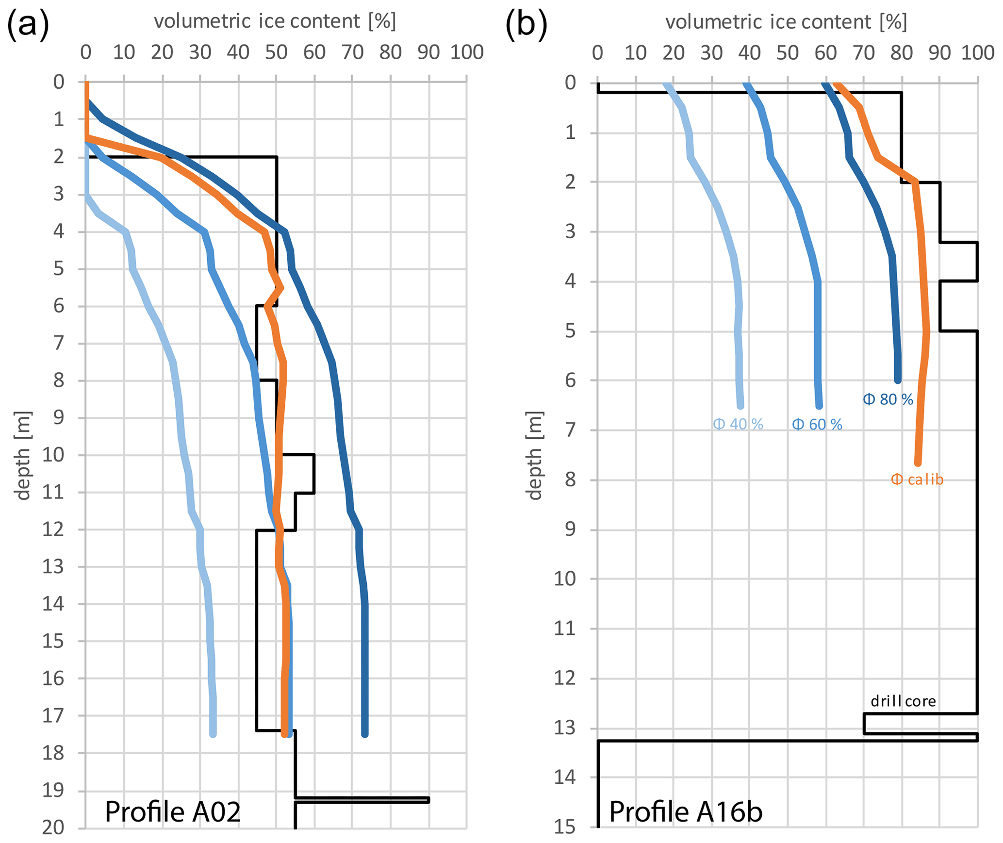
Figure 13 Comparison of ground truthing information from a drill core (black line) with 4PM-derived ground ice volumes at the borehole position of profiles A02 (a) and A16b (b). The ground truthing estimates of the ground ice content are based on an in situ evaluation of the drill cores, and the error is estimated at ±5 %. The blue lines correspond to 4PM runs based on homogeneous porosity models with Φ=40 %$/$60 %$/$80 % (as used for the ZOIs), and the orange line shows the 4PM result after calibration of the porosity model with ground truthing data. The 4PM model discretization is 0.5 m.

5.2 Ice content of rock glaciers

Ground ice is present in the majority of all profiles, with ice contents ranging from a few percent by volume to clearly supersaturated conditions within various rock glaciers (Fig. 3, Table 3). At sites with shallow sediment cover, small ice lenses are frequently present, which appear in the tomograms in the form of local resistive anomalies (see Table 3 and Appendix, Fig. B2), and could be validated through various test pits and natural outcrops. Based on the estimates drawn from the 4PM simulations (considering the 60 % and 80 % porosity models), the rock glaciers with resistivity maxima > 100 kΩm (RG I) within our study areas show on average ground ice contents between 35 % and 55 % by volume and thicknesses of the ice-rich layer of 3 to 25 m but with considerable spatial heterogeneity (see minimum and maximum estimates for the thickness of the ice-rich layer in Fig. 11a or the example in Fig. 5). Our results further suggest that the detected maximum ice contents within the ZOIs (35 %–75 %) roughly correspond to the general assumption on average ice contents within active rock glaciers found in the literature (40 %–60 %; see Arenson and Springman, 2005; Barsch, 1996), which implies, however, that this assumption may tend to overestimate mean ground ice contents on a landform scale. Care therefore has to be taken regarding general up-scaling approaches for quantitative estimates of the total ground ice content within a rock glacier. Several studies of the hydrologic role of rock glaciers in the Andes used an estimate of 50 % volumetric ice content as the mean value for rock glacier bodies (e.g. Brenning, 2005; Perucca and Angillieri, 2011; Rangecroft et al., 2015). This commonly used estimate is often justified by borehole core data from rock glaciers elsewhere (e.g. Haeberli et al., 1988; Mühll and Holub, 1992). However, boreholes are usually drilled at promising locations for massive ground ice occurrences, and the recovery of undisturbed samples with high ice contents is easier than sampling ice-poor samples. Therefore, results from boreholes are often biased towards ice-rich conditions and hence do not represent mean conditions for the entire landform. Estimates of volumetric ice content using a homogeneous value of 50 % can therefore easily lead to over-estimations.

In addition, published estimates of total ground ice volumes within rock glaciers have been based on simplified relations between the surface area and average rock glacier thickness (i.e. area–thickness relations introduced by Brenning, 2005). Figure 14 compares the area–thickness estimates according to the approach by Brenning (2005) with our geophysics-based estimates for the rock glaciers of our study. This comparison suggests that the thickness of the ice-rich permafrost layer as inferred from geophysical data is in most cases considerably smaller than the one approximated from commonly applied area–thickness relations (see Azócar and Brenning, 2010; Janke et al., 2017; Rangecroft et al., 2015). Only for a few of the very ice-rich landforms (e.g. E17 or A16b) do the two approaches show comparable results. In addition, areal extents of rock glaciers are often not clear and very difficult to determine (Brardinoni et al., 2019; RGIK, 2020), especially in the case of complex landforms combining multiple rock glacier generations, resulting in a significant source of error when applying any rock glacier area–thickness correlation.

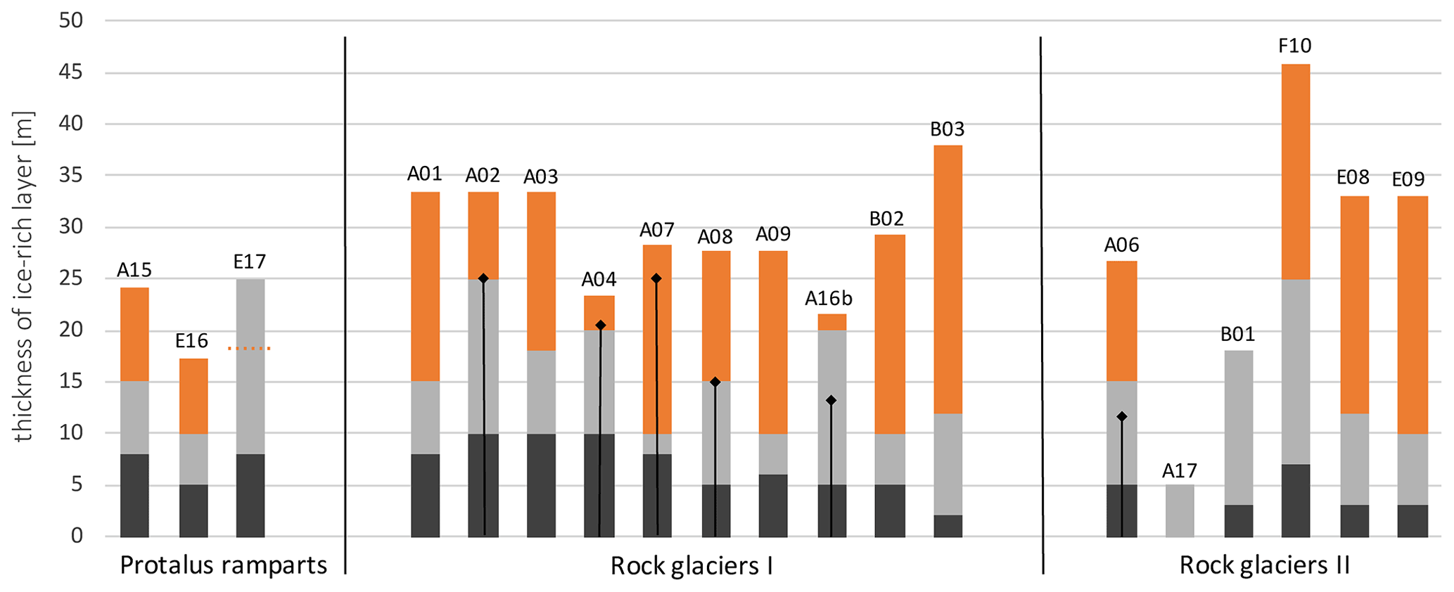
Figure 14 Comparison of the minimum (black) and maximum (grey) thickness of the ice-rich layer of rock glaciers (as in Fig. 4) with the estimated rock glacier thickness according to the area–thickness relation based on Brenning (2005) (orange) for selected rock glaciers and protalus ramparts. Brenning's approach has not been applied to A17 and B01, which are strongly degraded or relict rock glaciers. For E17, the area–thickness relation revealed a slightly smaller thickness (dashed orange line) than the geophysical maximum value. Vertical black lines illustrate the permafrost thickness revealed from borehole evidence, where available.

Although previous assumptions of ground ice content within rock glaciers (40 %–60 %; e.g. Brenning, 2005) roughly correspond to our field-based results, this is only true for their ice-rich zone. As rock glacier bodies also consist of zones with considerably smaller ice contents (see Appendix, Fig. B1), large-scale model studies using the above-mentioned area–thickness relations will introduce a bias towards overestimation of total ice content with respect to total area. In the companion paper, Mathys et al. (2021) propose a new upscaling approach of geophysics-based estimates of the ice volume per landform, which is compared to standard approaches using area–thickness scaling and constant ground ice contents per rock glacier. Similar to our results presented in Fig. 14 they find lower total ground ice volumes in rock glaciers when estimates are based on geophysical data in the field compared to simplified rock-glacier–ice-content relations.

5.3 Ice content of other landforms

In contrast to remote-sensing-based approaches, which can only delineate rock glaciers as indirect representations of permafrost bodies with unknown relevance for the hydrological cycle (Azócar and Brenning, 2010), the geophysics-based approach presented in this study is not restricted to rock glaciers but allows the estimation of ground ice content in a variety of landforms that constitute the periglacial belt (see Sect. 4.2 and 4.3). Neglecting landforms other than rock glaciers in most studies is due to the invisibility of their ground ice content from space (and during site visits) and the corresponding difficulties in obtaining field data from remote areas. Rough approximations indicate that even thin ice-rich layers in permafrost slopes at high elevations (e.g. Fig. 9) may add up to similar ice volumes per catchment as present in catchments in zones where individual rock glaciers are present and only a medium probability of permafrost exists.

To investigate this hypothesis, we upscaled the geophysics-based ice content estimates to the landform scale for two sites where ground truthing data are available. Based on geophysical results from six different profiles on a sediment slope (D03, D04, D05, D06, D07, D08) and three different profiles from a rock glacier (A01, A02, A03), the average thickness and ice content of the ice-rich layer of both landforms was approximated in terms of a lower-bound and an upper-bound estimate. Figure 15 shows the two landforms and the lower- and upper-bound estimates of the thickness of the ice-rich layer, as well as the estimated total ground ice volumes for the sediment slope and the rock glacier. The area of the rock glacier is approximately 0.11 km², which is about 10 times smaller than the considered area of the colluvial slope (∼ 1 km²), but the rock glacier is expected to have a substantially thicker ice-rich layer of 10–15 m, compared to 0.5–1.5 m for the sediment slope. The perimeter for the colluvial slope indicated in Fig. 15 hereby represents an area of 1 km² within a larger and well-studied region and is only used to illustrate the spatial dimension of a 1 km² colluvial slope in the landscape and its quantitative comparison with the rock glacier site regarding total ground ice content. For a more detailed analysis of upscaling issues, we refer to the companion paper (Mathys et al. 2021).

Assuming an average volumetric ice content of 50 % for the ice-rich layer at both sites leads to an approximated lower-bound estimate of the total ice volume of 250 000 m³ for the sediment slope and 550 000 m³ for the rock glacier. Considering the upper-bound estimate, i.e. the upper-bound average value for the thickness of the ice-rich layer (as opposed to its maximum within the landform), estimated volumes are comparable with 750 000 m³ for the sediment slope and 825 000 m³ for the rock glacier. This indicates that even thin ice layers in sediment slopes can contain similar ice volumes per catchment as rock-glacier-dominated catchments. A more detailed analysis of this hypothesis using a newly developed upscaling approach is presented and discussed in the companion paper (Mathys et al., 2021).

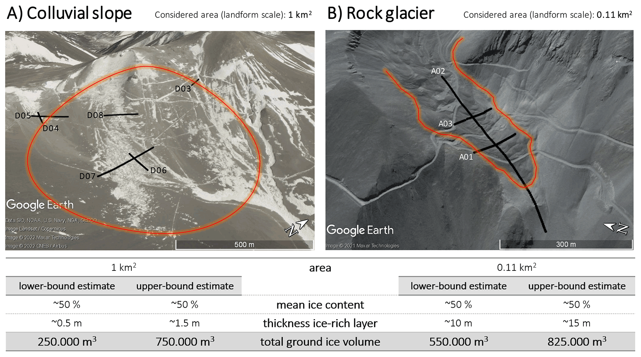
Figure 15 Estimated total ice content of (a) a colluvial slope area containing profiles D03–D08 versus (b) a rock glacier area (profiles A01–A03). Map data: perspective images from © Google Earth (2022).

6 Conclusion and outlook

Based on more than 50 geophysical surveys from various regions in the Central Andes, this study demonstrates the value of geophysical surveys (a) to detect ice-rich permafrost occurrences in various landforms (also beyond prominent forms such as rock glaciers) and (b) to estimate ground ice volumes in permafrost regions. The added value of combined ERT and RST surveys lies in an increased reliability of the interpretation (e.g. regarding the identification of bedrock) and the potential for ice content quantification through coupled petrophysical relationships such as within the four-phase model.

The availability of various ground truthing data (cores from boreholes, test pits, natural outcrops) in this study allows the validation of the geophysical results for many cases. The good agreement between independent validation data and interpreted geophysical profiles confirms the detection of ice-rich layers in various non-rock-glacier permafrost landforms, emphasizing the value of geophysical data in the scientific debate on the role of ice-rich permafrost in the hydrological cycle. Further, we observe a substantial intra- and inter-site heterogeneity of the thickness of the ice-rich layer(s) and ice volumes, which is often wrongly inferred from visual inspections alone. Purely remote-sensing-based approaches can provide valuable first-order estimates in the absence of ground-based data. However, geophysics-based estimates on ground ice content have been shown to allow for more accurate assessments. The data set presented in this paper is therefore one of the first available extensive sets of field-based and validated data regarding the presence and total quantities of ground ice in the Central Andes.

The analysis of 52 ERT and 24 RST profiles within this study confirmed that ice-rich permafrost is not restricted to rock glaciers but is also observed in non-rock-glacier permafrost slopes in the form of interstitial ice, as well as layers with excess ice, resulting in substantial ice contents (e.g. D09, D04, C07) which can be close to the volumes observed in rock glaciers (e.g. in the case of profile D09). Consequently, non-rock-glacier permafrost landforms, whose role for local hydrology has so far not been considered in remote-sensing-based approaches, may, depending on the catchment size of the watershed, be similarly relevant in terms of ground ice content on a catchment scale and should not be ignored when quantifying the potential hydrological significance of permafrost.

On the other hand, a realistic estimate of ground ice volume is only the first step towards the evaluation of the hydrological importance of permafrost within a catchment. Further factors, such as (a) different response times of permafrost landforms to observed and projected atmospheric changes in the Central Andes and (b) the dominance of the relevant hydrological processes (e.g. melting vs. sublimation and discharge vs. evaporation), play a decisive role in the annual contribution to total run-off to downstream water resources from degrading permafrost (or to evaporation and sublimation) (e.g. Rivera et al., 2017). According to Duguay et al. (2015) the contribution of degrading permafrost to the total run-off of a catchment is difficult to measure, and hence quantify, and therefore remains basically unknown. Without a reliable determination of these factors (e.g. by measuring or modelling the full energy balance over permafrost areas; see, for example, Harrington et al., 2018), the relevance of permafrost for the hydrological cycle remains strongly speculative. Preliminary modelling approaches and conceptual considerations suggest that this is negligible and would be non-measurable in the arid Andes (Arenson et al., 2013, 2022), and a recent analysis of mass balance rates of ice masses in the Argentinian Central Andes confirms that rock glaciers showed almost zero mass balance rates from 2000 to 2018 (Ferri et al., 2020). However, no publications exist so far that have specifically calculated the contribution of rock glaciers to streamflow in the semi-arid Andes of Chile (Schaffer et al., 2019). Studies from other mountain environments (e.g. the European Alps; Marmy et al., 2016; Scherler et al., 2013) have shown that, depending on the snow cover and surface characteristics, the degradation of rock glaciers can be a very slow process because of the extremely efficient insulating effect of the active layer (coarse blocks) and the latent heat effect. Haeberli (1985) approximated the time needed for the complete decay of ice-rich permafrost in rock glaciers under a warming climate to be of the order of centuries to millennia, and Krainer et al. (2015) showed that ∼ 10 000-year-old permafrost ice persisted until today even during warm periods of the Holocene. The quantitative contribution of melting ground ice of degrading permafrost in rock glaciers to the annual discharge from the catchment can therefore be very small (Harrington et al., 2018; Krainer et al., 2015; Pruessner et al., 2021), and the relative contributions from other ice-poor permafrost landforms without blocky surfaces and thin but widespread ground ice layers still remain unknown. The geophysical data set presented in this study may therefore serve as input for modelling studies on the overall amount of ground ice present within the periglacial belt and estimates regarding the relative contributions of rock glacier and non-rock-glacier ground ice to run-off in the semi-arid regions of the Central Andes.

Appendix A: Background information for the 4PM modelling

The main principles for the four-phase model are as follows (see Hauck et al., 2011; Mewes et al., 2017):

• the electrical mixing rule (Archie's law), which was found empirically by Archie (1942) and later theoretically confirmed by, for example, Sen et al. (1981);

• an extension to a four-phase medium of the seismic time-averaged approach for P wave velocities (modified based on Timur, 1968); and

• the necessary assumption that the sum of all volumetric fractions of the ground is equal to one.

Based on these principles, the 4PM uses the following equations to determine the volumetric fractions of ice (f_i), water (f_w), and air (f_a) for a given porosity model Φ(x,z) ($\mathrm{\Phi }=\mathrm{1}-f_{\mathrm{r}}$; f_r being the rock content):

$$\begin{array}{}\text{(A1)}& {\displaystyle }{f}_{\mathrm{w}}={\left({\displaystyle \frac{a{\mathit{\rho }}_{\mathrm{w}}(\mathrm{1}-f_{\mathrm{r}}{)}^n}{\mathit{\rho }(\mathrm{1}-f_{\mathrm{r}}{)}^m}}\right)}^{\mathrm{1}/n},\text{(A2)}& {\displaystyle }\begin{array}{rl}{f}_{\mathrm{i}}& ={\displaystyle \frac{v_{\mathrm{i}}{v}_{\mathrm{a}}}{v_{\mathrm{a}}-v_{\mathrm{i}}}}\left[{\displaystyle \frac{\mathrm{1}}{v}}-{\displaystyle \frac{f_{\mathrm{r}}}{v_{\mathrm{r}}}}-{\displaystyle \frac{\mathrm{1}-f_{\mathrm{r}}}{v_{\mathrm{a}}}}\right.\\ & \left.+{\left({\displaystyle \frac{a{\mathit{\rho }}_{\mathrm{w}}(\mathrm{1}-f_{\mathrm{r}}{)}^n}{\mathit{\rho }(\mathrm{1}-f_{\mathrm{r}}{)}^m}}\right)}^{\mathrm{1}/n}\left({\displaystyle \frac{\mathrm{1}}{v_{\mathrm{a}}}}-{\displaystyle \frac{\mathrm{1}}{v_{\mathrm{w}}}}\right)\right],\end{array}\text{(A3)}& {\displaystyle }\begin{array}{rl}{f}_{\mathrm{a}}& ={\displaystyle \frac{v_{\mathrm{i}}{v}_{\mathrm{a}}}{v_{\mathrm{i}}-v_{\mathrm{a}}}}\left[{\displaystyle \frac{\mathrm{1}}{v}}-{\displaystyle \frac{f_{\mathrm{r}}}{v_{\mathrm{r}}}}+{\displaystyle \frac{\mathrm{1}}{v_{\mathrm{i}}}}(f_{\mathrm{r}}-\mathrm{1})\right.\\ & \left.-{\left({\displaystyle \frac{a{\mathit{\rho }}_{\mathrm{w}}(\mathrm{1}-f_{\mathrm{r}}{)}^n}{\mathit{\rho }(\mathrm{1}-f_{\mathrm{r}}{)}^m}}\right)}^{\mathrm{1}/n}\left({\displaystyle \frac{\mathrm{1}}{v_{\mathrm{w}}}}-{\displaystyle \frac{\mathrm{1}}{v_{\mathrm{i}}}}\right)\right],\end{array}\end{array}$$

where a (= 1 in many applications), m (cementation exponent), and n (saturation exponent) are empirically determined parameters (Archie, 1942), ρ_w is the resistivity of the pore water, v_r, v_w, v_a, and v_i are the theoretical P wave velocities of the four components, and ρ(x,z) and v(x,z) are the inverted resistivity and P wave velocity distributions, respectively.

The pore water resistivity (ρ_w) and the porosity Φ are the most sensitive for the calculation of the ice and water content (Hauck et al., 2011). In the absence of exact information around these parameters, e.g. through borehole or laboratory data, there is an uncertainty involved in the modelling approach. The choice of the parameters and the corresponding uncertainty has been addressed in several publications and can be found in, for example, Pellet et al. (2016) and Mewes et al. (2017).

Appendix B: Overview of the entire geophysical data set

Table B1 Data quality overview of the geophysical data. Abbreviations: n= number of quadrupoles; n_filtered = remaining quadrupoles after filtering; RMS = root mean square error.

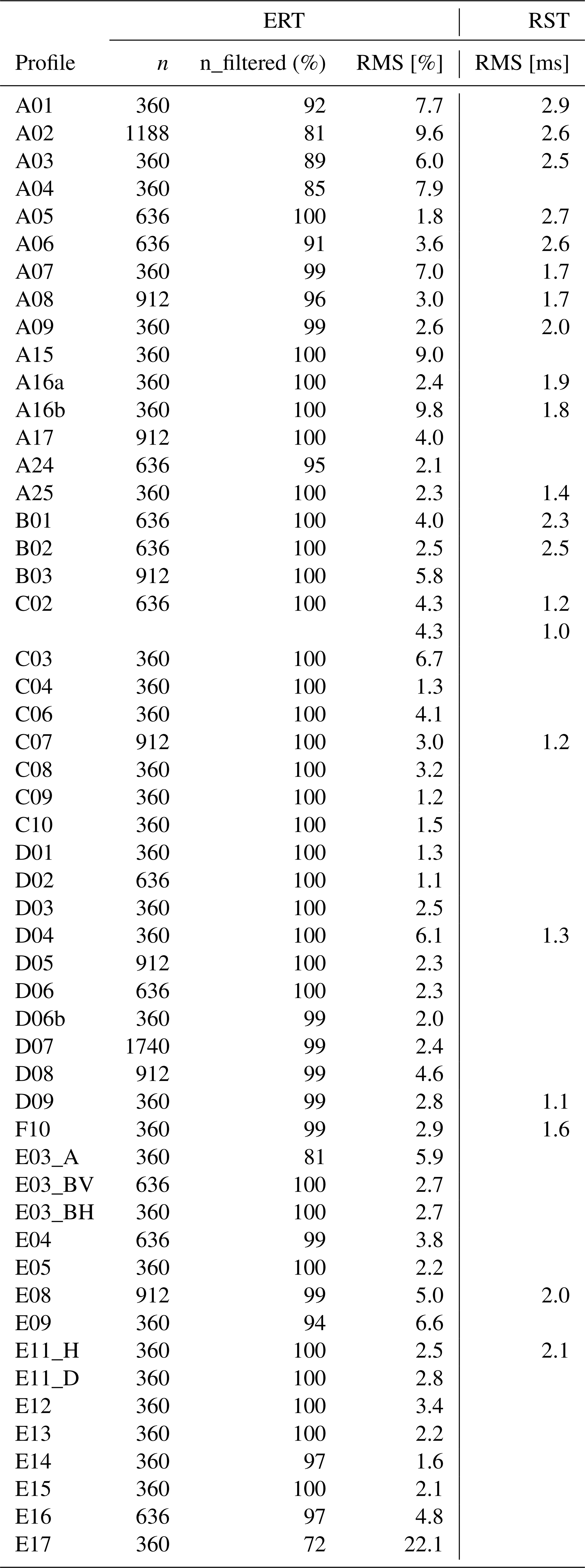
Figure B1 Inverted tomograms of all ERT profiles from coarse-blocky sites (same spatial and colour scales), sorted by landforms.

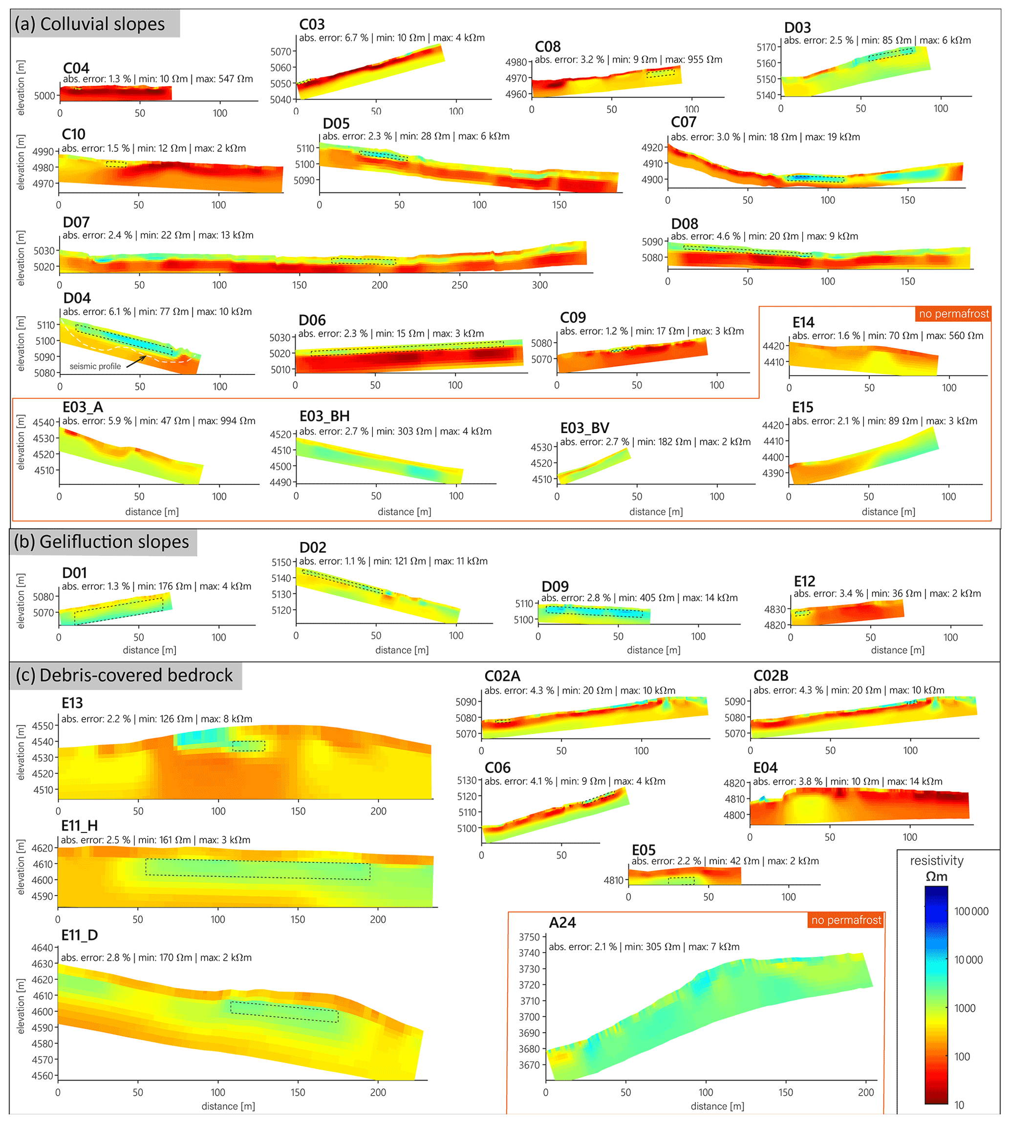
Figure B2 Inverted tomograms of all ERT profiles from sediment and bedrock sites (same spatial and colour scales), sorted by landforms. The position of the seismic profile shown in Fig. 9 is highlighted in profile D04.

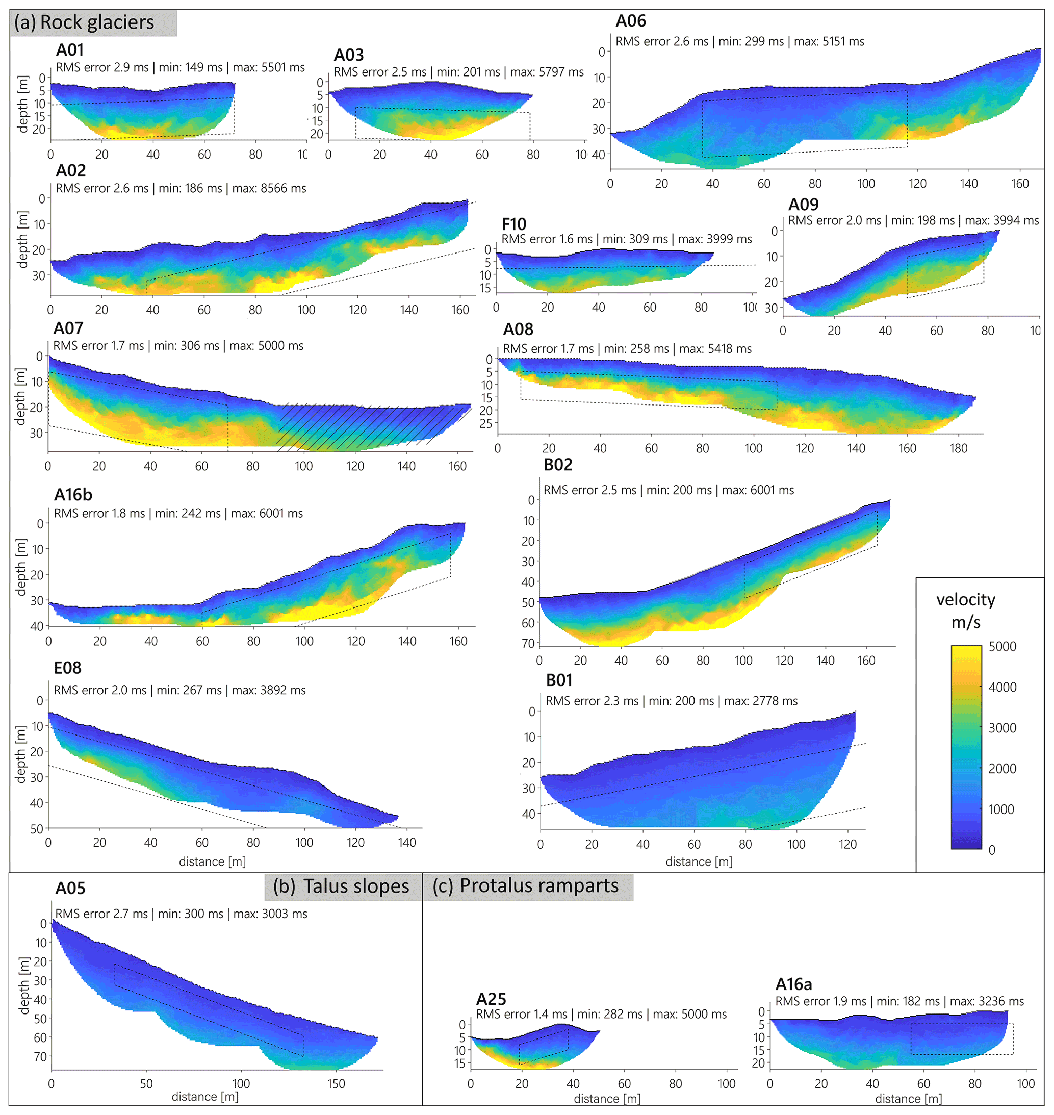
Figure B3 Inverted tomograms of all RST profiles from coarse-blocky sites (same scales and colour scales), sorted by landforms.

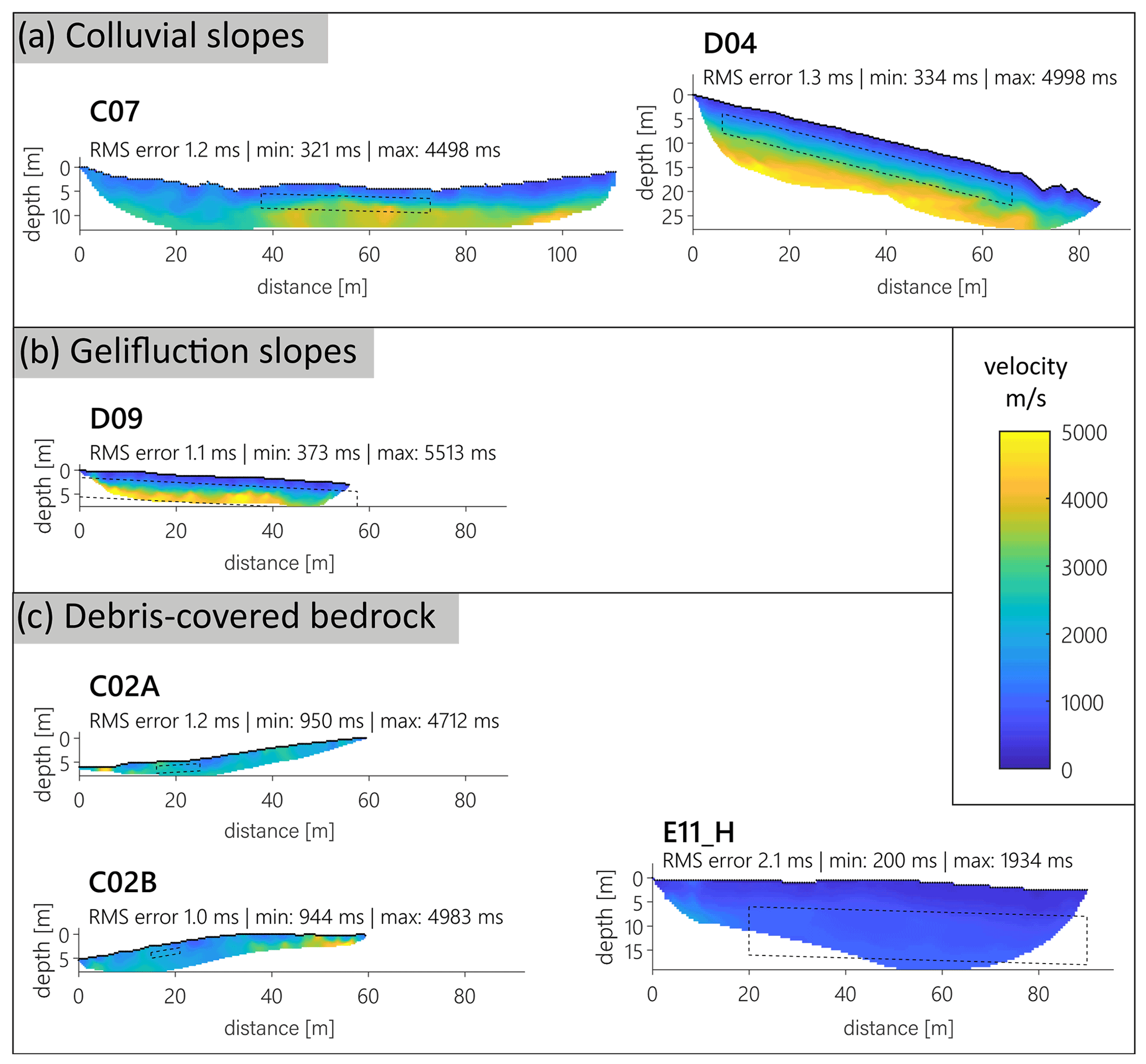
Figure B4 Inverted tomograms of all RST profiles from sediment and bedrock sites (same scales and colour scales), sorted by landforms.