Three different glacier surges at a spot: what satellites observe and what not

In the Karakoram, dozens of glacier surges occurred in the past 2 decades, making the region a global hotspot. Detailed analyses of dense time series from optical and radar satellite images revealed a wide range of surge behaviour in this region: from slow advances longer than a decade at low flow velocities to short, pulse-like advances over 1 or 2 years with high velocities. In this study, we present an analysis of three currently surging glaciers in the central Karakoram: North and South Chongtar Glaciers and an unnamed glacier referred to as NN9. All three glaciers flow towards the same small region but differ strongly in surge behaviour. A full suite of satellites (e.g. Landsat, Sentinel-1 and 2, Planet, TerraSAR-X, ICESat-2) and digital elevation models (DEMs) from different sources (e.g. Shuttle Radar Topography Mission, SRTM; Satellite Pour l’Observation de la Terre, SPOT; High Mountain Asia DEM, HMA DEM) are used to (a) obtain comprehensive information about the evolution of the surges from 2000 to 2021 and (b) to compare and evaluate capabilities and limitations of the different satellite sensors for monitoring surges of relatively small glaciers in steep terrain. A strongly contrasting evolution of advance rates and flow velocities is found, though the elevation change pattern is more similar. For example, South Chongtar Glacier had short-lived advance rates above 10 km yr⁻¹, velocities up to 30 m d⁻¹, and surface elevations increasing by 170 m. In contrast, the neighbouring and 3-times-smaller North Chongtar Glacier had a slow and near-linear increase in advance rates (up to 500 m yr⁻¹), flow velocities below 1 m d⁻¹ and elevation increases up to 100 m. The even smaller glacier NN9 changed from a slow advance to a full surge within a year, reaching advance rates higher than 1 km yr⁻¹. It seems that, despite a similar climatic setting, different surge mechanisms are at play, and a transition from one mechanism to another can occur during a single surge. The sensor inter-comparison revealed a high agreement across sensors for deriving flow velocities, but limitations are found on small and narrow glaciers in steep terrain, in particular for Sentinel-1. All investigated DEMs have the required accuracy to clearly show the volume changes during the surges, and elevations from ICESat-2 ATL03 data fit neatly to the other DEMs. We conclude that the available satellite data allow for a comprehensive observation of glacier surges from space when combining different sensors to determine the temporal evolution of length, elevation and velocity changes.

1 Introduction

Glacier surges in the Karakoram are widespread (e.g. Sevestre and Benn, 2015) and have been thoroughly documented using historic literature sources and time series of satellite images (Copland et al., 2011; Bhambri et al., 2017; Paul, 2020). A large number of publications provide insights into decadal elevation changes (e.g. Bolch et al., 2017; Berthier and Brun, 2019; Brun et al., 2017; Gardelle et al., 2013; Rankl and Braun, 2016; Zhou et al., 2017) and mean annual flow velocities (e.g. Dehecq et al., 2015; Rankl et al., 2014) at a regional scale. Using various satellite datasets, several studies have also investigated individual glacier surges at high temporal resolution (e.g. Bhambri et al., 2020; Mayer et al., 2011; Paul et al., 2017b; Quincey et al., 2015; Round et al., 2017; Steiner et al., 2018).

This increasing interest is in part due to the hazard potential of glacier surges, in particular when river damming creates lakes that might catastrophically drain in so-called glacier lake outburst floods (GLOFs) with far-reaching impacts (e.g. Bazai et al., 2021; Bhambri et al., 2019 and references therein; Iturrizaga, 2005) but also due to the increased availability of satellite data for characterizing surges in detail (e.g. Dunse et al., 2015; King et al., 2021; Nuth et al., 2019; Rashid et al., 2020; Wang et al., 2021; Willis et al., 2018). The still limited understanding of surges in the Karakoram region (e.g. Farinotti et al., 2020) and the high diversity of observed surge characteristics (e.g. Bhambri et al., 2017; Hewitt, 2007; Paul, 2015; Quincey at al., 2015) also contribute to the recent efforts. These studies found that both main types of glacier surges can be found in the Karakoram, sometimes side by side: the Alaska type, which might be triggered by a change in the basal hydrologic regime, creates pulse-like surges of a short duration (2–3 years), whereas the thermally controlled Svalbard type has often active surge durations of many years (e.g. Jiskoot, 2011; Murray et al., 2003; Raymond, 1987; Sharp, 1988). Although the physical reasons for the differences and variability in surges in the Karakoram are yet unknown (e.g. glacier properties, thermal regime, mass balance history), many glaciers in the Karakoram have surged repeatedly, sometimes at surprisingly constant intervals and over centuries (e.g. Bhambri et al., 2017; Paul, 2020). On average, surges in the central Karakoram repeat after 40 to 60 years, but intervals can range from less than 20 to more than 80 years.

In the thermally controlled case, it is sometimes difficult to distinguish a regular advance from a surge as the transition can be gradual (Lv et al., 2020). Whether an advance (stimulated by a positive mass budget) is indeed a surge might be determined by comparison with the behaviour of neighbouring glaciers. As thresholds on advance rates or ice flow speed-up might not be efficient to distinguish (slow) surges from advances in the Karakoram, the typical mass redistribution pattern of a surge (from an upper reservoir to a lower receiving zone) as obtained from differencing digital elevation models (DEMs) acquired a few years apart (e.g. Gardelle et al., 2013) is a more reliable identifier (Lv et al., 2019; Goerlich et al., 2020). Usually, the surface in the upper regions of a glacier does not lower significantly during a regular advance (Lv et al., 2020). A further method to discriminate surges from a usual advance is related to a strong increase in crevassing and development of shear margins. However, these are only visible in very-high-resolution satellite images or time series of synthetic aperture radar (SAR) data (Leclercq et al., 2021).

In this study, we present (a) a comparative analysis of the ongoing surges of three glaciers in the central Karakoram: North and South Chongtar Glacier and a small unnamed glacier referred to here as NN9. We present a comparative analysis of their changes in length, advance rates, flow velocities and surface elevations to elucidate the respective similarities and differences in surge behaviour. As a second aim of this study, we (b) investigate the feasibility of various satellite sensors and DEMs to follow the temporal evolution of the surges comprehensively. Included are optical (Sentinel-2, Landsat, Planet CubeSats) and SAR imaging sensors (Sentinel-1, TerraSAR-X); altimeter data from ICESat-2; and DEMs from the Shuttle Radar Topography Mission (SRTM), the Satellite Pour l'Observation de la Terre (SPOT), the High Mountain Asia DEM (HMA DEM), and the Advanced Spaceborne Thermal Emission and reflectance Radiometer (ASTER). The latter is an external dataset provided by Hugonnet et al. (2021).

2 Study region

The study region is located in the central Karakoram, north of the Baltoro Glacier, at about 35.94^∘ N, 76.33^∘ E (Fig. 1). East of the study region stands the second-highest mountain in the world, the 8611 m high K2. Slopes of the surrounding terrain are very steep, and snow avalanches from the surrounding rock walls are a major source of glacier nourishment. Mass changes over the past 20 years derived from satellite data using the geodetic method show more or less constant near-zero mass budgets in the study region (Hugonnet et al., 2021), confirming the continuation of the “Karakoram Anomaly” (i.e. the balanced mass budgets) in this region (Farinotti et al., 2020).

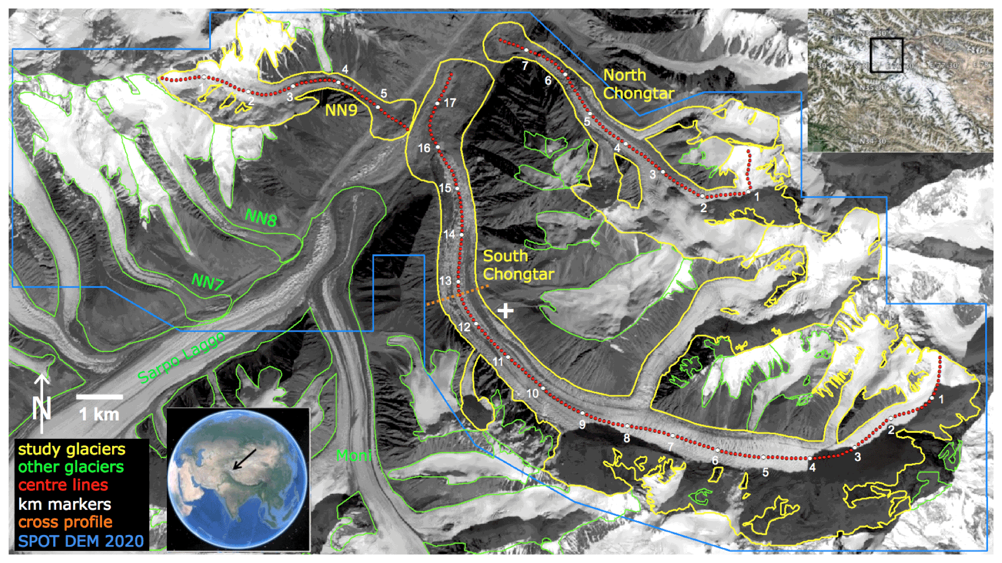
Figure 1 Overview of the study region showing the location of the Karakoram Mountains (inset, lower left) and of the study region (inset, upper right), outlines of the investigated glaciers (yellow) and other glaciers (green), centrelines (red), kilometre (km) markers (white), cross-profile line (orange), and extent of the SPOT 2020 DEM perimeter (blue). The white + near the centre marks the coordinates 35.9^∘ N, 76.34^∘ E. The satellite image in the background is the Landsat 8 panchromatic band acquired on 21 October 2020. Credits: Landsat – http://earthexplorer.usgs.gov (last access: June 2021); the two insets are screenshots from Google Earth (© Google Earth 2018).

Most precipitation in the study region is brought by westerly airflow during winter, but the monsoon brings moist air from the south-east also during summer (Maussion et al., 2014), falling as snow at the high elevations of the rock walls surrounding most glaciers. However, due to the good protection from nearly all directions, the amount of snowfall in the study region is limited, and a dry continental climate can be expected (e.g. Sakai et al., 2015). As surge-type glaciers are abundant (Copland et al., 2011; Bhambri et al., 2017), and repeat intervals are comparably short (Paul, 2020), several glaciers in the Karakoram are typically actively surging at any given time.

The three glaciers investigated here (North and South Chongtar, NN9) have mean elevations around 5500 m and are surrounded by mountain ridges with elevations between 6000 and 7500 m above sea level. South Chongtar Glacier (shortened to South Chongtar in the following) is the largest, with an area of ∼ 31 km² and a length of more than 14 km at minimum extent, but it has a narrow tongue with a near-constant width of about 800 m. The glacier is mainly east–west-oriented in its upper part, bending towards south–north near the terminus. North Chongtar lies north of South Chongtar and is connected to it in its accumulation area. It flows from south-east to north-west, covers an area of ∼ 10 km², has a length of 4.5 km at minimum extent and is about 400 m wide. The unnamed glacier NN9 is located on the opposite side of the main valley and flows roughly from west to east. The glacier is about 3.5 km long at minimum extent, with an area of 4 km² and a ∼ 300 m wide tongue. Table 1 summarizes further characteristics and topographic properties.

Table 1 Characteristics of the three investigated glaciers using outlines modified from the GAMDAM2 glacier inventory (Sakai et al., 2019) and digitized in this study. Elevations refer to the SRTM DEM. Values given for “min/max” refer to the minimum and maximum extent of a glacier shortly before and after a surge, respectively.

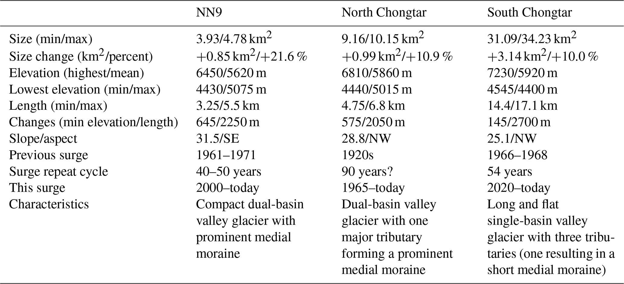
At their historically recorded maximum extent the three glaciers reach Sarpo Laggo Glacier, a compound-basin valley glacier with a size of 122.3 km². This glacier experienced a massive surge shortly before 1960 (Paul, 2020) and a smaller, more internal one (i.e. not reaching the terminus) between 1993 and 1995 (e.g. Paul, 2015; Bhambri et al., 2017). According to Paul (2020), South Chongtar had a rapid advance during a surge that started in 1966 with a short active phase of about 2 years followed by a quiescent phase with continuous down-wasting and retreat. During this surge it partly compressed the ice from Sarpo Laggo and deformed a moraine from the Moni Glacier tributary (see Fig. 1), leaving an impressive surge mark. In contrast, North Chongtar started advancing about 55 years ago but has not yet reached Sarpo Laggo. The Shipton map from 1937 (Shipton et al., 1938) shows North Chongtar in contact with it, indicating that the terminus might reach it again. The glacier NN9 had its last surge from about 1961 to 1971 (leaving a small surge mark on Sarpo Laggo) and retreated in its quiescent phase until 2000, when it started to advance slowly. The two glaciers to the south of NN9 (NN7 and NN8 in Paul, 2020) both surged around 1955 and again in 1998 and 1980, respectively. NN8 also surged after 2002, indicating a surge cycle of only 20–25 years. The next surge of NN8 can thus be expected in a few years, at least if environmental conditions prevail.

3 Datasets

In this section, we describe the satellite and auxiliary datasets used to derive time series of glacier outlines, surface flow velocities and elevation changes in the study region. Figure 2 shows the temporal coverage of each dataset and the periods selected for the analysis. Changes in glacier extent have been mapped for the active (advance) phases of the three glaciers, starting with Landsat Multispectral Scanner (MSS) images from 1973 for North Chongtar Glacier. The earliest datasets used to derive flow velocities and elevation changes were acquired in 2000, based on the Landsat 7 Enhanced Thematic Mapper plus (ETM+) panchromatic band and the SRTM DEM, respectively.

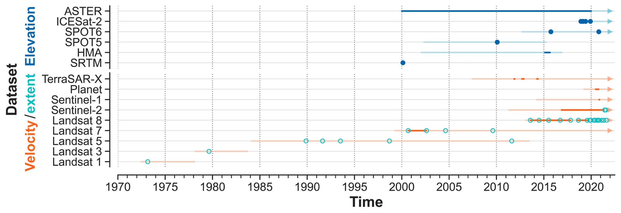
Figure 2 Timeline of the temporal coverage of the satellite sensors used (light line) and dates and time series selected for the analysis (lines or dots). Lines and dots in dark blue indicate the elevation change analysis, orange lines the velocity analysis, and green dots the glacier extents.

3.1 Glacier extent and centrelines

We used glacier outlines from the updated Glacier Area Mapping for Discharge from the Asian Mountains (GAMDAM2) inventory by Sakai (2019) as a starting point for all glacier extents. This dataset was locally improved (removing rock outcrops and seasonal snow) using a Landsat 8 image acquired on 21 October 2020 (Fig. 1). Given the unknown final length of the glaciers, we digitized likely maximum extents for the three glaciers, avoiding overlapping polygons in their terminus regions. The virtual extents were guided by maximum extents of previous surges described by Paul (2020).

Changes in extent were derived from time series of spatially consistent Landsat data (MSS, TM, ETM+ and Operational Land Imager (OLI)) from path-row 148-35. The slightly shifted Sentinel-2 scenes (sensor: Multi Spectral Imager, MSI) from tile 43SFV were used to bridge a gap in availability of cloud-free Landsat scenes after February 2021. The shift of about 50 m was manually subtracted to obtain a correct time series of length changes. The spatial resolution of the optical sensors used for this purpose is 60 m (MSS), 30 m (TM), 15 m (ETM+, OLI) and 10 m (MSI). The list of satellite scenes used for determination of geometric changes (outlines, length changes) is given in Table S1 of the Supplement.

The centrelines for NN9 and South and North Chongtar were manually digitized starting from the highest points of each glacier down to the virtual maximum extent. The centrelines were divided into equidistant points of 100 m, at which values for velocity and elevation were extracted.

3.2 Flow velocity

Time series of optical and SAR data were used to derive glacier flow fields (see Table S2). Landsat 7 and 8 scenes, Sentinel-2, and TerraSAR-X (TSX) were used (Fig. 2) to determine pre-surge flow velocities of South Chongtar and advance- and surge-phase velocities for all glaciers. Images from Planet CubeSats were used for a comparison of results with Sentinel-2 and some gap-filling in the time series rather than for a full documentation of the active surge of South Chongtar. The related optical images were acquired in summer or autumn for the pre-surge phase of South Chongtar and all year during its surge (Table S2).

From TSX, co-registered single-look slant range complex (SSC) images acquired in StripMap mode, with across- and along-track resolution of up to 3 m, are used. The selected image pairs are from two different tracks; cover the study region in the descending direction; and were acquired in winter 2011, autumn 2012 and spring 2014 (Table S2). Time series of Sentinel-1 single-look complex (SLC) data acquired in interferometric wide (IW) swath mode were used to test its feasibility to derive flow velocities and to create an animation of the surge that is unobstructed by clouds. The Sentinel-1 IW SLC data have a nominal ground resolution of 5 m × 20 m.

3.3 Elevation information

To follow the three glaciers' elevation changes before and during the surge, we analysed several DEMs from both optical and SAR sensors (Table 2). We used the following DEMs with known acquisition dates: the SRTM1 DEM at 1 arcsec (∼ 30 m) resolution from February 2000 (USGS, 2017), a SPOT5-HRS DEM from October 2010 (Gardelle et al., 2013; we used their version 2 for rugged areas), a SPOT6 DEM from October 2015 (Berthier and Brun, 2019) and a SPOT7-derived DEM from October 2020 that was generated for this study. In addition, we used the HMA DEM mosaic (Shean, 2017) as a reference for DEM co-registration analysis due to its superior spatial resolution and accuracy over stable terrain (off-glacier) compared to the other DEMs (Fig. S1 in the Supplement). The HMA DEM is composed of various DEM datasets mostly acquired during 2015 (February, April, July and August) in this region. Elevation values along the centrelines are extracted from these DEMs, and DEM differences are calculated for the periods 2000–2010, 2010–2015 and 2015–2020. For comparison, we also analysed elevation changes derived from ASTER time series by Hugonnet et al. (2021). These provide additional information about the periods 2000–2004 and 2005–2009 (full calendar years) as well as from 2000 to 2019, before the surge of South Chongtar.

Table 2 Overview of the DEMs used to determine elevation changes in the glaciers in the study region and the additional ICESat-2 dataset.

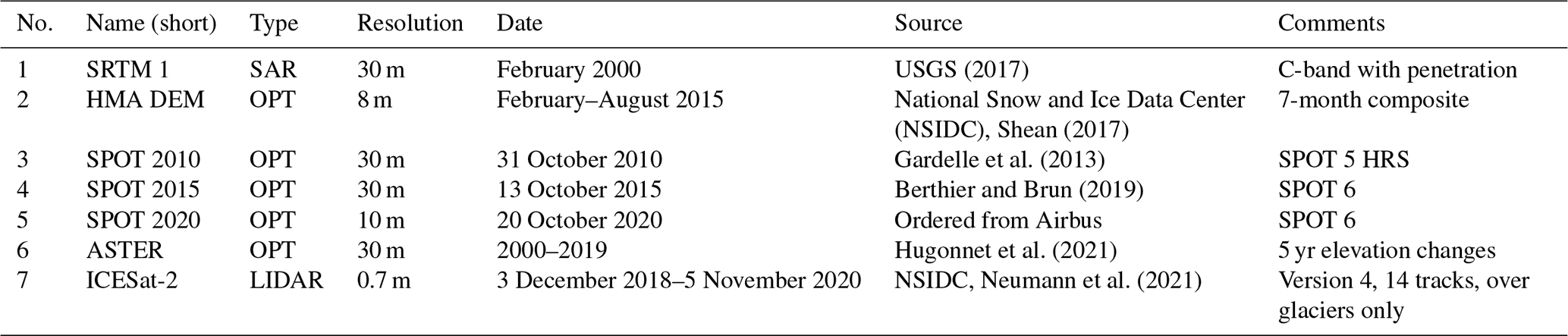
We also analysed whether altimetry data from ICESat-2 could be used to reveal elevation changes at a higher temporal resolution. The Advanced Topographic Laser Altimeter System (ATLAS) instrument on board ICESat-2 has been acquiring elevation profiles at a 91 d temporal resolution since October 2018. Each satellite overpass results in three beam pairs that are separated by 3.3 km and 90 m between and within pairs, respectively (Markus et al., 2017). The ICESat-2 ATL06 dataset provides geolocated land ice surface heights with 40 m spatial resolution in profile direction. Figure S2 shows the ATL06 dates and elevations of data points crossing North and South Chongtar and the two closest repeating pairs of tracks on South Chongtar. Due to the systematic off-pointing at mid-latitudes, ICESat-2 tracks are not repeated exactly in our study area, and the ATL06 data alone proved too sparse, both geographically and temporally, for further analysis of the surges.

The ICESat-2 ATL03 Global Geolocated Photon Data product (Neumann et al., 2021), from which the ATL06 dataset is a higher-level derivative, provides surface elevation measurements from individual photons every 0.7 m along the elevation profiles, revealing details of the surface topography of the glaciers. The ICESat-2 surface elevations fall into the time gap of the DEMs between 2015 and 2020, thus providing additional temporal information on the surge development. In total, we found 42 intersections with the centrelines of the three investigated glaciers: 23 on South Chongtar (from seven dates), 13 on North Chongtar (from six dates) and 6 on NN9 (from three dates).

4 Methods

4.1 Glacier extent

The timing of the selected images used to digitize glacier extents varies strongly depending on the advance rates. To have at least a 2-pixel change in frontal position (which is sufficient for sound change detection), it varies from several years for the slow advance of North Chongtar to about 16 d for the surge phase of South Chongtar. For North Chongtar also the spatial resolution of the sensor matters to some extent as 2 pixels translates to a required advance of 120 and 60 m for MSS and TM, respectively. Due to frequent cloud cover, different scenes had to be used for the individual glaciers (Table S1 in the Supplement). For the digitization, the polygon referring to the virtual maximum extent of each glacier was split into a multi-polygon by digitizing the smaller extents visible on the respective satellite images.

Length changes between two terminus positions from t₁ and t₂ were derived manually using the distance tool in ArcGIS. Several values were obtained for each change and a suitable average assigned (values usually varied by about ±10 m). We only used the Landsat 7 and 8 time series for this as the Landsat Collection 1 data had a spatial shift compared to Sentinel-2 (e.g. Paul et al., 2016). The length change values from t₁ to t₂ were divided by the temporal difference (t₂−t₁), converted to mean annual advance rates, and assigned to the date that is halfway between t₁ and t₂. Cumulative changes were obtained by summing up the individual length changes.

4.2 Velocities

Flow velocities typically span 2 to 3 orders of magnitude, e.g. from < 0.1 m d⁻¹ for near-stagnant glaciers to > 10 m d⁻¹ during a surge. When using offset-tracking (e.g. Strozzi et al., 2002) for both Sentinel-1 and TSX or image correlation for optical data (Debella-Gilo and Kääb, 2012), this range can to some extent be accounted for by varying the search window size or the time between the acquisition dates of the image pair. If glaciers with very different flow velocities are in the study region, it might be required to use images from different dates for the analysis or an adaptive search window (Debella-Gilo and Kääb, 2012). In the following, we describe some basics of the processing lines applied for optical and SAR sensors.

The normalized cross-correlation algorithm implemented in the correlation image analysis software (CIAS; Kääb and Vollmer, 2000) is used to calculate the glacier surface displacement between optical satellite image pairs (Fig. S3 illustrates the workflow). The satellite images were not co-registered as we assume that they are corrected for topographic distortion, and therefore the displacement calculated between two images is the actual horizontal displacement without any influence of topography. To check co-registration, abundant stable terrain was included in the correlation. The displacements are estimated at a spatial resolution of 100 m, while the size of the search area is set in relation to the maximum displacement estimated between two satellite scenes. Dividing the displacement by the temporal difference between the image pairs (Table S2) gives velocity in metres per day.

With optical data, clouds, cast shadows and changes in snow cover lead to false detections or biased measurements of the calculated displacement fields. These mismatches are removed in post-processing by setting a threshold of the maximum correlation coefficient (< 0.5) and velocity. For Sentinel-2 data, elevated objects such as clouds are detected by applying CIAS between band 4 and band 8 of the same Sentinel-2 scene. The calculated perspective displacements (both bands are recorded at slightly different positions of the sensor) are then used to mask the clouds. For all satellite data, spatial filtering based on a moving median window and temporal filtering are applied to remove additional outliers and noise (Fig. S3).

Surface flow velocities for TSX data were derived by an iterative offset-tracking technique developed for SAR data (Wuite et al., 2015). This method does not require coherence and is thus also capable of acquiring flow velocity data over longer time spans and in regions with fast flow. The method is based on cross-correlation of templates in SAR amplitude images and provides both the along-track and line-of-sight velocity components from a single image pair. We used a template size of 96 × 96 pixels for generating velocity maps with 50 m grid spacing and applied a 9×9 inverse-distance median filter in the post-processing step to remove outliers and fill in small gaps. For Sentinel-1, the same method was applied, but tests with various image template sizes were performed with an image pair acquired on 4 and 16 November 2020 during the peak of the surge (Fig. S4).

4.3 Elevation data

We used the MicMac software to generate the SPOT 2020 DEM from the raw imagery (Rupnik et al., 2017). The pre-processing of all DEMs follows the standard processing steps for DEM differencing: all DEMs were projected to UTM 43N (EPSG 32643), elevations were vertically transformed to the WGS 84 ellipsoid, and DEMs were co-registered to the HMA DEM using OPALS (Pfeifer et al., 2014). Specifically, we applied least-squares matching to estimate the full 3D affine transformation parameters that minimize the errors with respect to the reference DEM over common stable areas. These were manually digitized off-glacier excluding slope values larger than 40^∘ (Fig. S5). Because of data voids, we also had to exclude large parts of the accumulation areas of some glaciers in the case of the SPOT 2010 and 2015 DEMs.

All DEMs were resampled, clipped, and aligned to the same 30 m grid and a high-resolution 5 m grid for the HMA DEM and SPOT 2020. We did not correct the SRTM DEM for microwave penetration into ice and snow (Gardelle et al., 2012) as the effect is small compared to the elevation differences caused by the surges and uncertain; i.e. it is not systematic, and any, for example, elevation-dependent correction cannot be justified either. Elevation values were extracted along the centrelines and subtracted from SRTM.

To estimate volume changes resulting from the surges, volume gain and loss (i.e. summing up all positive and negative values within the tongues) were calculated for each glacier tongue with adjusted extents and glacier-specific epochs (Fig. S5). For comparison, we included the glaciers NN7 and NN8 (see Fig. 1) in the analysis as they also surged during the study period.

As the ICESat-2 ATL06 datasets did not provide useful results, only the ATL03 dataset was further processed using Python libraries GeoPandas (Jordahl et al., 2021), Rasterio (Gillies et al., 2021a) and Shapely (Gillies et al., 2021b). The photon elevations were filtered to only retain elevation samples classified as likely land or ice surfaces (parameters signal_conf_ph and signal_conf_ph_landice > 1) and classified into glacier and off-glacier samples using maximum glacier outlines. On the bright glacier surface, both the weak and strong laser beams yield sufficient photon returns for complete elevation profiles. This is less true for moraines and rocky areas (profile 3 in Fig. S6), where the weak beam yields considerably fewer surface returns.

Elevation values were sampled for all elevation points (containing a DEM cell), and the AMES stereo pipeline (version 2.7.0; Shean et al., 2016) was used to co-register the elevation profiles (only off-glacier samples) with the already-co-registered DEMs used in this study (no co-registration offset was found). The profiles were intersected with the glacier centrelines to compare the ATL03 elevation samples with the DEMs. The median of all elevation samples on each profile within a 10 m buffer from the centreline is used as surface elevation at the intersection points.

4.4 Uncertainties

The uncertainty in the length change data has been determined by measuring for each glacier and each time step different points at the terminus. From the range of values, a reasonable mean value was determined manually. Glacier terminus positions were digitized only once and used only for a qualitative illustration (outline overlay) of the changes; i.e. we have not explicitly calculated uncertainties in glacier extents. As a range of sensors with different spatial resolutions is used for the digitizing (e.g. Landsat MSS, ETM+, OLI and Sentinel-2), the uncertainty varies with the sensor.

Based on the assumption that measurement errors over glaciers and other terrain are common (Paul et al., 2017a), we assessed the uncertainties in glacier flow velocities from stable-terrain velocity observations, where flow velocities are supposed to be zero, using the same stable areas as used for DEM co-registration (Fig. S5). Uncertainties are derived as measures of median and a robust standard deviation based on the median absolute deviation (MAD), which is a bit less sensitive to outliers (e.g. Dehecq et al., 2015). Co-registration accuracy of the DEMs was computed from elevation differences calculated over stable terrain (off glacier) with slopes smaller than 40^∘ (Fig. S5).

5 Results

5.1 Changes in glacier extent and morphology

In Fig. 3 the temporal evolution of terminus positions is depicted as an overlay of extents showing slow advances of NN9 (starting in 2000) and North Chongtar (since 1973) along with a rapid advance of South Chongtar (starting mid-2020). For better visibility, the retreat phase of South Chongtar from 2000 to mid-2020 is not shown. Snapshots of the geometric evolution can be found in Fig. S7 for the time period before the surge of South Chongtar (1993–2019) and in Fig. S8 for the time during its surge (2020–2021). The related cumulative length changes for all three glaciers are shown in Fig. 4a for their advance phases, whereas Fig. 4b only shows advance rates for the glaciers NN9 and North Chongtar (they were out of scale for South Chongtar).

Figure 3 Temporal evolution (colour-coded dates) of glacier extent for the three glaciers (NN9, North Chongtar, South Chongtar) investigated here. For comparison, the displacement of the terminal lobe of Moni Glacier from 2000 to 2020 is also shown (blue arrow). “Last” is referring to 30 September 2021; the + sign near the centre marks the coordinates 35.93^∘ N, 76.34^∘ E. Background: Sentinel-2 image acquired on 16 July 2021 with bands 8, 4 and 3 as RGB (Copernicus Sentinel data 2021).

South Chongtar entered its quiescent phase after its 1966/67 surge and exhibited constant thinning with limited frontal retreat over several decades. After 30 years (in 2000) the former surge lobe was still largely ice-filled, though increasingly debris-covered. Driven by further thinning, a clear retreat of the terminus (remaining clean ice) became visible after 2000, reaching about −800 m by 2009 and −2300 m by mid-2020. During this retreat phase, its middle part always showed some residual flow, i.e. it was not completely stagnant. In 1993 a deformation of the medial moraine started moving forward, about 300 m by 2009 and 500 m by 2019.

In 2017, a new surge developed with the typical funnel-shaped appearance of the front. While the lowest part of the glacier was still thinning and retreating in 2019, the surge front reached the terminus in July 2020, and the front started advancing by about 3 km in 10 months (Fig. 4a) with advance rates of up to 12.6 km yr⁻¹ (35 m d⁻¹) in early November 2020. During this time the lower part widened massively, and the entire surface became heavily crevassed. The front advanced into its former surge mark on Sarpo Laggo Glacier and pushed the ice surrounding it towards the opposite side of the valley. By June 2021 advance rates decreased considerably, but the terminus was still advancing.

Figure 4 Terminus changes for the investigated glaciers. (a) Cumulative length changes (the retreat phase of South Chongtar before 2020 is not shown), (b) advance rates.

North Chongtar on the other hand advanced at a more or less constant rate of 30 m yr⁻¹ until 2004, when it passed a total of 800 m since 1973 (earliest MSS image; see Table S1). A very high-resolution satellite image from 2001 is available in Google Earth and shows some crevassing near the terminus but not a surging glacier. There is no indication of a meltwater stream leaving the glacier snout. After 2005, advance rates increased linearly, and we assign this as the onset of the surge phase. This increase resulted in a nearly completely crevassed surface and widespread shear margins. Both are also visible in the 15 m resolution Landsat panchromatic bands and, even better, in very-high-resolution images from 2011 and 2016 available in Google Earth. In 2013 the terminus reached a step in the valley slope, creating a deep transverse crevasse that seemed to separate the lowest part of the tongue but actually did not. By 2021 nearly the entire surface was still crevassed, and the glacier had advanced by a further 1600 m since 2004, i.e. 2.4 km in total.

The small valley glacier NN9 slowly retreated until 1998 and started advancing a year later at about a constant rate of 40 m yr⁻¹ until 2016 (Fig. 4). Up to this year, its lowest parts had some crevasses but looked otherwise like a usual advancing glacier. This changed a year later when the glacier thickened considerably, developed shear margins and started advancing at a much higher rate of up to 1000 m yr⁻¹ in 2021, indicating the start of the surge phase. The increasingly crevassed surface also became visible in Sentinel-2 images and with the 15 m Landsat 8 band. The total advance from 1999 to 2018 was 800 m followed by a further 500 m until June 2021. In July the frontal advance accelerated further, reaching nearly 3 km yr⁻¹ in August 2021, whereby the lower part of the tongue separated from the main glacier and slid down the remaining kilometre in about a month. More ice is following from higher elevations, possibly leading to some interaction with the still-advancing terminus of South Chongtar.

5.2 Flow velocities

5.2.1 NN9 and North Chongtar

Selected flow velocity maps for the two glaciers are shown in Fig. 5, and related velocity profiles along the centreline of the main trunk can be seen in Fig. 6a and b for NN9 and North Chongtar, respectively. The ca. 300–400 m wide tongue of NN9 is at the edge of the possibilities for deriving flow velocities with offset-tracking (and a 100 m grid) from the optical sensors, but the high resolution of TSX StripMap acquisitions provides near-complete spatial coverage (Fig. 5b). Due to local cloud cover, several of the optical image pairs selected for South Chongtar could not be used for NN9 and North Chongtar.

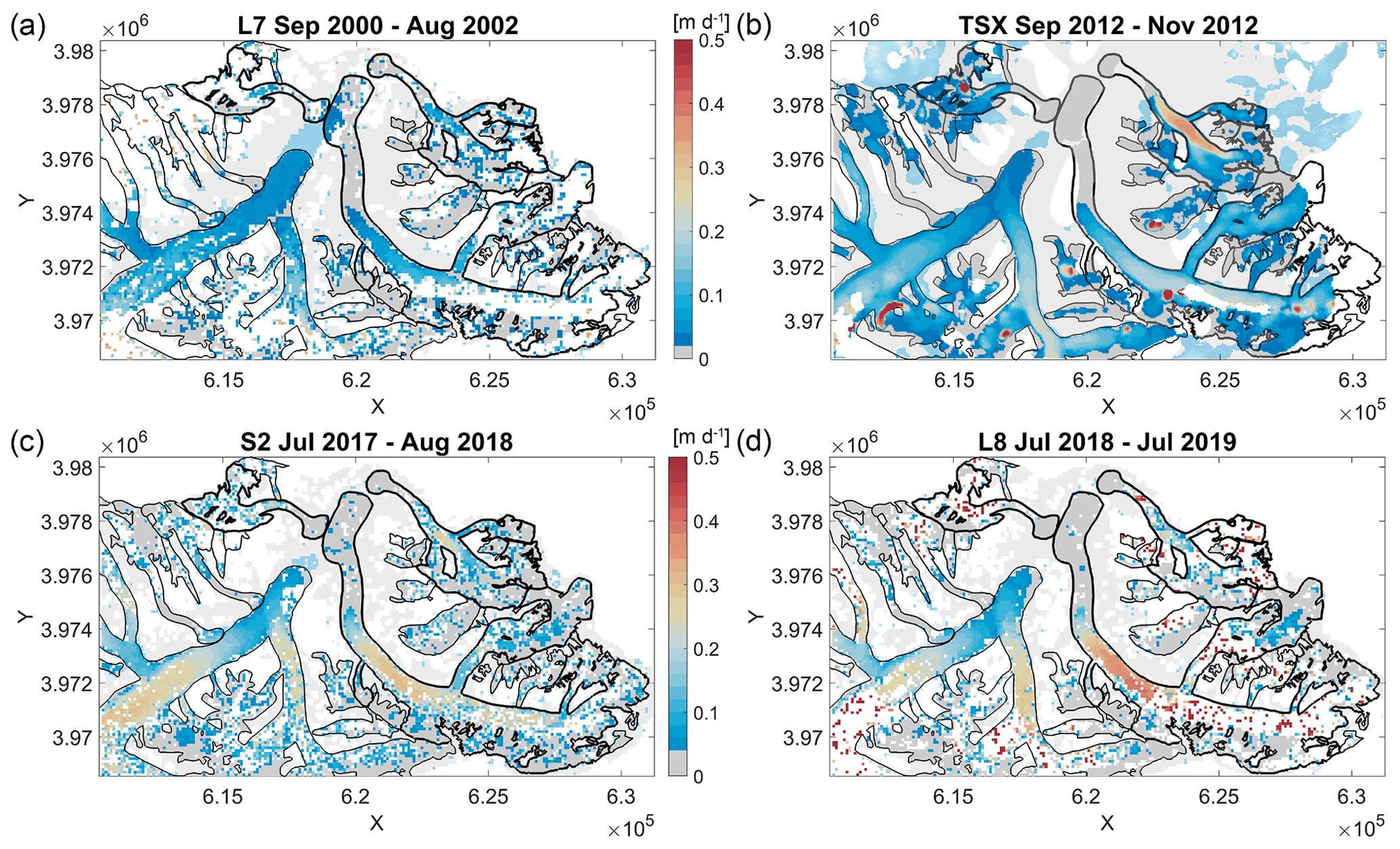
Figure 5 Temporal evolution of 2D surface flow velocities for the three glaciers before 2020 derived from (a) Landsat 7, (b) TerraSAR-X, (c) Sentinel-2 and (d) Landsat 8. The dates of the compared images are given at the top of each panel. Grey values refer to velocities smaller than the uncertainty (see Table S2), i.e. < 0.01 m d⁻¹ for panels (a) and (b) and < 0.02 m d⁻¹ for (c) and (d).

Though scattered, the values derived from Landsat 7 (Fig. 5a), Sentinel-2 (Fig. 5c) and Landsat 8 (Fig. 5d) look reasonable. Pre-surge values are around 0.1 m d⁻¹ with Landsat 7 (2000–2002) and TSX (2011 and 2012) and a bit higher (up to 0.2 m d⁻¹) with Sentinel-2 in 2017 (Fig. 6a). Afterwards values in the lower part of NN9 (between 2.5 and 4 km) start increasing to 0.4 m d⁻¹, reaching 0.8 m d⁻¹ between August and October 2020. The upper glacier started accelerating in autumn 2020 with a near-linear increase up to the terminus (Fig. 6a), indicating surge activation in the lower part of the glacier. The increased crevassing of NN9 is also visible in the higher intensity values of the Sentinel-1 animation towards the latest images (see Supplement).

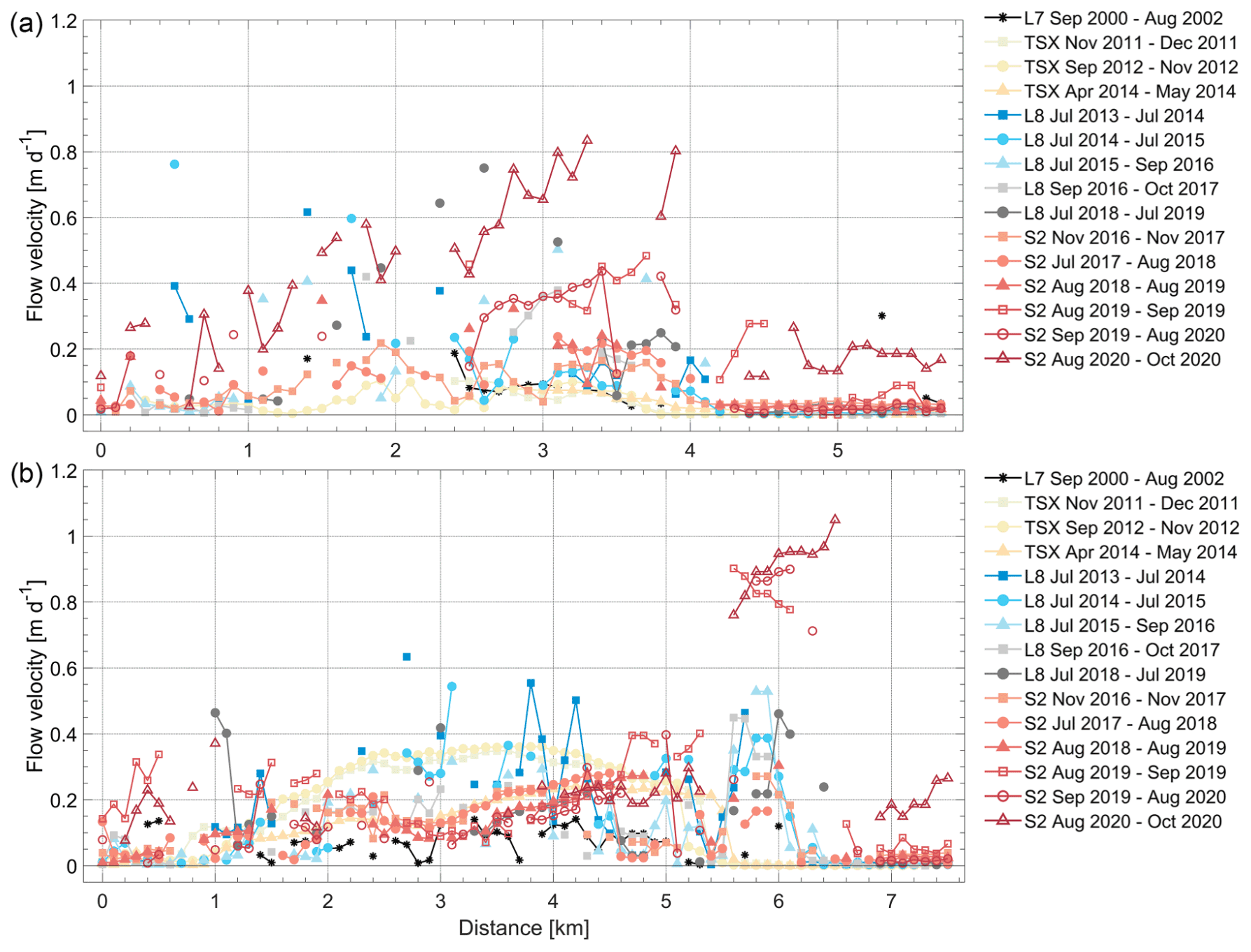
Figure 6 Temporal evolution of 1D flow velocities along a centreline starting at the highest point of each glacier for (a) glacier NN9 and (b) North Chongtar. Satellite names: L7 and L8 – Landsat 7 and Landsat 8, TSX – Terra-SAR-X, S2 – Sentinel-2.

For the larger North Chongtar, a slightly better coverage can be obtained from the optical sensors than for NN9. The most homogenous flow fields are derived by TSX (Fig. 5b), indicating higher flow velocities of up to 0.4 m d⁻¹ in its lower two-thirds up to the terminus in 2012. The profiles in Fig. 6b from Landsat 7 show similar values. Velocities derived from Sentinel-2 between 2016 and 2019 are lower in the region from 3 to 5.5 km. There is a zone with very low velocities between 4.5 and 5 km and acceleration further down. From August 2019 to October 2020 flow velocities are between 0.8 and 1 m d⁻¹ near the terminus, indicating that this region is fast-flowing and advancing, whereas the upper regions are still moving with 0.2 to 0.4 m d⁻¹.

5.2.2 South Chongtar

The much larger South Chongtar glacier was adequately captured by the optical sensors so that a more continuous flow field could be derived (Fig. 5), and pre-surge flow evolution could be followed in detail (Fig. 7a). Comparing the maps in Fig. 5, a slow but steady increase in flow velocities from 2000 to mid-2019 over large parts of the glacier can be seen, starting at about 0.15 m d⁻¹ and ending at 0.4 m d⁻¹. These values are similar to the other two glaciers but affect a larger region. The temporal evolution shown in Fig. 7a confirms this observation: pre-surge flow velocities are highest (up to 0.4 m d⁻¹) near the middle of the glacier (around 8 to 10 km) and decrease gradually to 0 m d⁻¹ at its highest and lowest points. In the region between 11 and 14 km the gradual increase in flow velocities can be followed from 2000/02 (with Landsat 7) to 2014 (with TSX). Mean annual values with Landsat 8 from 2013 to 2014 match perfectly with mean monthly TSX values from April to May 2014. Landsat 8 velocities from 2013 to 2016 and Sentinel-2 from 2016 to 2019 show the continuation of the slow velocity increase over the entire glacier length, reaching 0.4 m d⁻¹ in 2018/19. A direct comparison with Landsat 8 over nearly the same period (grey dots in Fig. 7a) is shown on top of the curve from Sentinel-2, indicating again a near-perfect match. In August 2019 the gradual increase changed, at first rapidly to 0.8 m d⁻¹ and then more slowly to 1.1 m d⁻¹, between September 2019 and June 2020. With the stagnant terminus still at 13.5 km, the strong velocity increase behind the front marks the onset of the surge around August 2019.

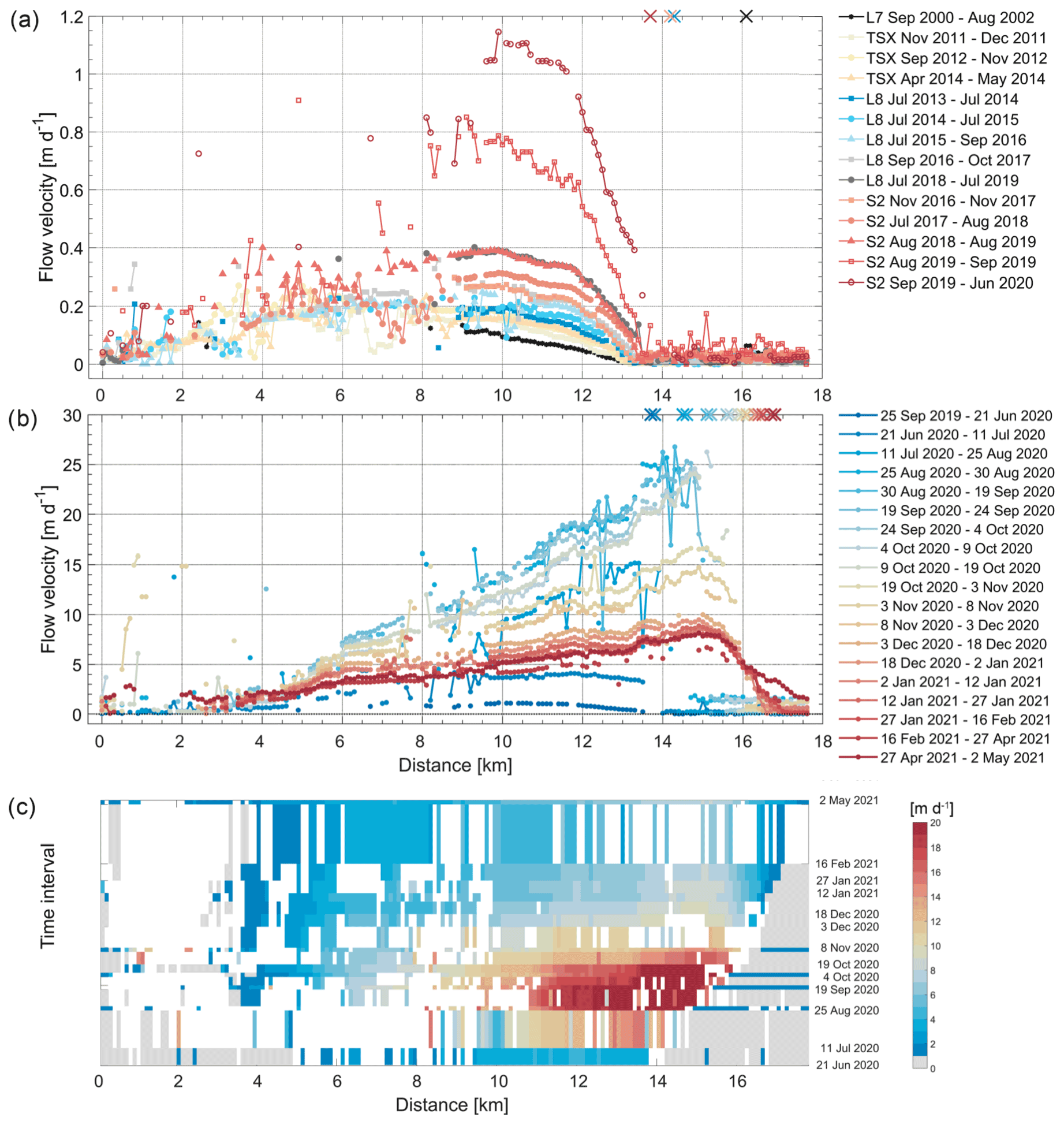
Figure 7 Temporal evolution of flow velocities for South Chongtar Glacier from its highest point to its terminus; its location is indicated by an “x” at the top of panels (a) and (b). (a) Pre-surge values along the centreline as derived from different satellites (for names, see Fig. 6). (b) As (a) but during the surge and derived from Sentinel-2 only. (c) Hovmöller diagram of the surge phase. In this plot grey values are below 1 m d⁻¹; white indicates no data.

The last curve from Fig. 7a is repeated in Fig. 7b (dark blue at the bottom) as we had to switch the scale for better visibility of velocities during the surge phase. Flow velocities increased to about 4 m d⁻¹ by July 2020. In August 2020 we could derive detailed flow fields from Sentinel-2 images acquired only 5 d apart. A sharp surge front with maximum velocities formed, reaching values of more than 25 m d⁻¹ in August/September 2020. With peak velocities near 30 m d⁻¹ as derived locally from Planet imagery (Fig. S10), South Chongtar Glacier had likely one of the highest flow velocities ever measured in the Karakoram region. Behind this maximum, flow velocities decreased about linearly back to km 3 along the centreline. When the surge front reached the terminus in July 2020, a rapid advance started (see Sect. 5.1). Velocities dropped to 15 m d⁻¹ by November 2020 and below 10 m d⁻¹ by January 2021. Afterwards, maximum velocities are found near km 15 and decreased only slowly at this location and over large parts of the glacier length (back to km 6) at about the same rate, indicating that the active surge was ongoing. Around km 10 along the centreline, velocity is still around 5 m d⁻¹ in early May 2021, or 40 times higher than during the quiescent phase (Fig. 7b). The related Hovmöller diagram for the surge phase in Fig. 7c confirms the strong pulse-like acceleration in August 2020 with a rapid decline afterwards. The corresponding 2D plots of flow velocities during the surge phase of South Chongtar (Fig. 8) also reveal the rapid velocity increase by September 2020 and the decrease afterwards.

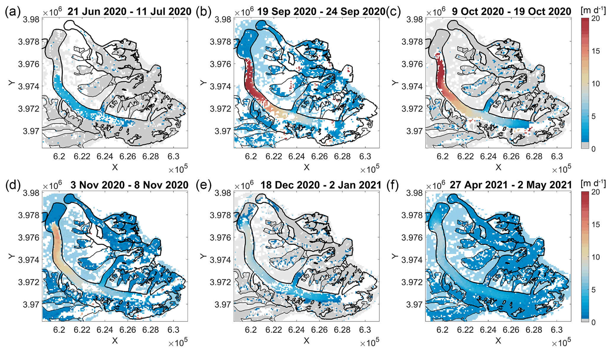
Figure 8 Temporal evolution of 2D flow velocities for South Chongtar Glacier during its surge as derived from Sentinel-2. The dates of the respective Sentinel-2 pairs are given at the top of each panel. Grey values refer to velocities smaller than 1 standard deviation (see Table S2), i.e. < 1 m d⁻¹ for panels (a) to (c) and < 0.5 m d⁻¹ for (d) to (f).

The spatial distribution of highest flow velocities of Fig. 8b and c are not symmetric to the centreline, indicating that the deformation-related maximum flow velocity in the centre of a glacier has reduced relevance here. This somehow counterintuitive behaviour indicates that during a surge, basal sliding is the process dominating over deformation. Other possibilities are a decreased resistance of the valley floor or because of the topography redirecting the mass flow from north-west to north. The cross-profile flow velocities (Fig. 9) reveal that this pattern persists throughout the entire surge.

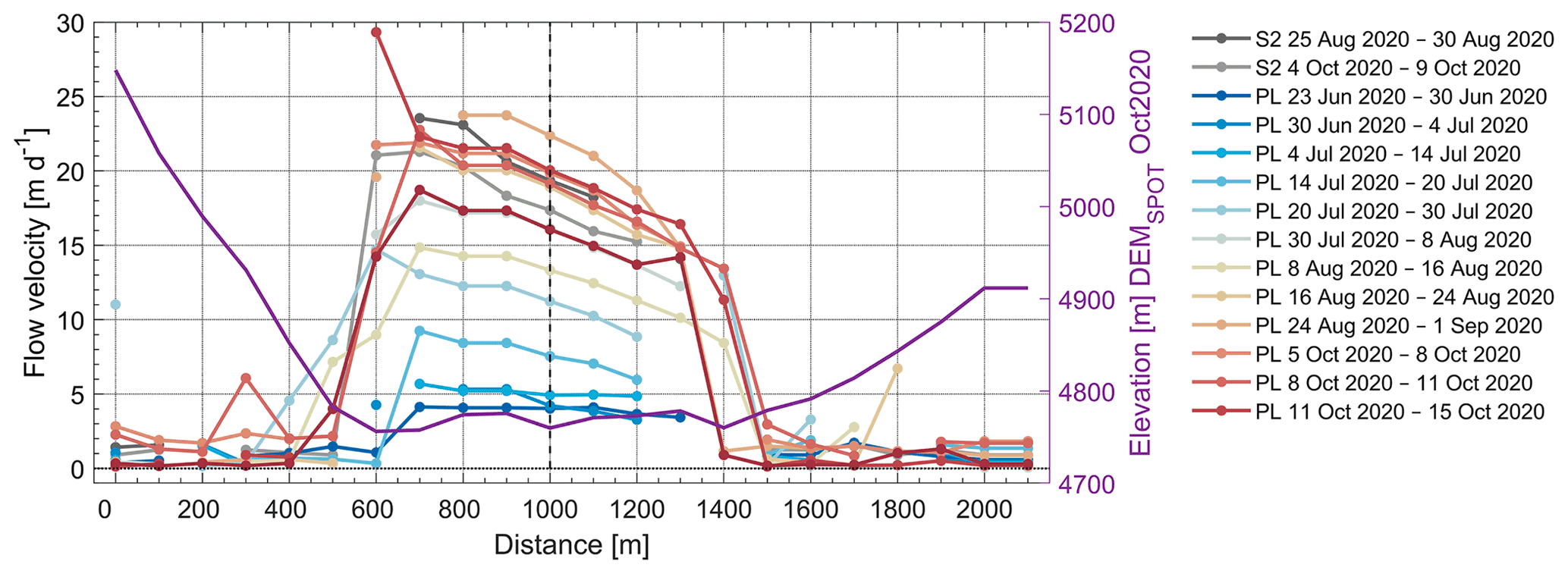
Figure 9 South-west to north-east cross-profile surface flow velocities for South Chongtar Glacier derived from Planet and comparison with Sentinel-2. The vertical dashed line indicates the location of the centreline. See Fig. 1 for location of the cross-profile.

5.3 Elevation changes

In the three panels of Fig. 10 we show differences in elevation between the SRTM DEM and the other four DEMs along the centrelines of the three glaciers. Additionally, differences from selected ICESat-2 ATL03 points are plotted. Figure 11 shows related elevation change maps for 2000–2010, 2010–2015, 2015–2020 and 2000–2020. DEM differences obtained from ASTER in an independent study (Hugonnet et al., 2021) have been used for comparison.

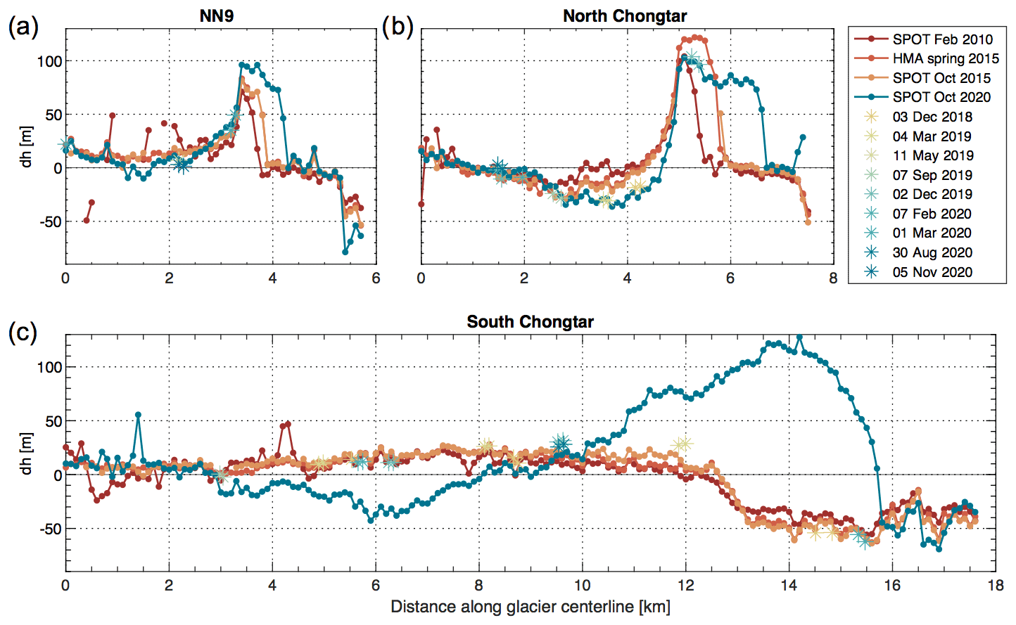
Figure 10 Elevation differences along the glacier centrelines with respect to the SRTM DEM from 2000 for the three investigated glaciers, namely (a) NN9, (b) North Chongtar and (c) South Chongtar glaciers. The star (*) markers and dates in the legend correspond to ICESat-2 elevation differences with respect to the SRTM DEM. Note that due to the different track locations, only some of the dates shown in the legend are present in each panel.

The elevation data for NN9 (Fig. 10a) show virtually no change in its upper part down to km 3.5, where the terminus was located in 2000. The ICESat-2 data add no further information here as all available data points are located in the upper part. Below this region, the “elevation gain” due to the advancing snout can be followed down to km 4.5 in 2020. The small region of elevation gain by the advancing tongue is also visible in each of the maps in Fig. 11. The elevation differences between the two high-resolution DEMs from 2015 and 2020 in Fig. 11c reveal some surface lowering in the upper part (about 10–15 m), but over the longer period 2000 to 2020 (Fig. 11d) this lowering nearly disappears (i.e. is smaller than the SRTM uncertainty). So for NN9 the typical mass transfer of a surge could not be observed until October 2020, and elevation changes look like expected for a usual advance rather than a surge.

For North Chongtar (Fig. 10b) the situation is similar, but a surface lowering of about 40 m can be observed at higher elevation. The SPOT data from October 2015 and ICESat-2 data points from December 2018 at km 4.2 indicate that the largest changes happened between 2015 and 2018. Accordingly, this change is well visible in the high-resolution 2015–2020 DEM difference (Fig. 11c) and the differences over the full 2000–2020 period (Fig. 11d). However, also here the elevation gain in the lower glacier part is comparably localized and largely due to the advance of the terminus.

South Chongtar shows profiles (Fig. 10c) and surface change patterns (Fig. 11) that are in line with a typical surge, maybe apart from the fact that the thickening of the upper glacier regions is limited. The 2000 to 2010 change map (Fig. 11a) shows a slightly bluish upper part and some artefacts. Over the longer 2000 to 2015 period the elevation gain from 4 to 12 km is about 20–30 m (Fig. 10c), but further down a significant surface lowering (> 50 m) can be observed between 13 and 18 km. This lowering is also visible in the 2D map of Fig. 11a, marking at its upper point the position where the active ice starts, i.e. where the surface lowering is compensated by the mass flux. The 2020 surge moved ice between 3 and 8 km towards its lower part between 10 and 16 km, causing a surface elevation decrease of 20–40 m in the reservoir zone and an increase of up to 130 m at km 14. This gives a 170 m high wall of ice moving down the valley at 1 m h⁻¹.

The ICESat-2 data points constrain the surface elevation evolution in time (Fig. 10c): the tongue was still only slightly thicker at 12 km in March 2019 as surface lowering of the upper part (at 5.7 km) had not started in February 2020, and the terminus had not advanced by March 2020. Between 6 and 14 km we find a smooth linear increase in the elevation differences (Fig. 10c) – but the ICESat-2 data points at 9.5 km show a slight surface lowering between December 2019 and August 2020, indicating that the surge front passed this part of the glacier already before the end of August 2000. The 2015 to 2020 elevation change map (Fig. 11c) reveals that elevation changes mostly occurred over this time period. Due to the opposite elevation change pattern before 2015, elevation changes over the full period 2000–2020 are less pronounced. The constantly down-wasting Sarpo Laggo Glacier in the valley floor shows an elevation loss of up to 100 m over this period.

5.4 Volume changes

In Table 3 the results of the calculated volume changes are listed, differentiated for the gain and loss part. They add some quantitative information over a larger part of the glacier surface (see Fig. S5). With the timing of the DEMs not always synchronous with the start or end of a surge, the calculated values can be underestimated due to the overlap of surge phases. For example, the volume gain in the lower part of South Chongtar from 2000 to 2020 includes the volume loss between 2000 and 2019. For this reason we only analyse the 2015 to 2020 changes for South Chongtar.

Table 3 Calculated volume changes (in cubic kilometres) for six glaciers and different periods as obtained from the respective DEMs. Numbers in italics denote results that might be impacted by artefacts. See Fig. S5 for the location of the zones used to determine volume changes.

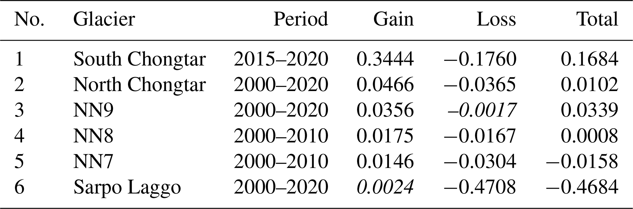
For NN9 no mass transfer from an upper region is found. We have a near-zero mass loss compared to a clear volume gain of 0.03 km³. For the continuous advance and surge of North Chongtar, the volume gain is a bit higher than the loss, resulting in a small overall volume gain over the full 20-year period (Fig. 11d). However, Fig. 11c reveals that compensation effects are included: between 2015 and 2020 some of the volume gain from the period before has already started thinning. The volume gain part for South Chongtar is about 10 times higher compared to North Chongtar and NN9. However, there is also considerable volume loss at higher elevations compensating about half of the gain. To put just the volume gains of these five glaciers (+0.46 km³) into perspective, the (uncompensated) volume loss of Sarpo Laggo Glacier over the full period (−0.47 km³) is the same.

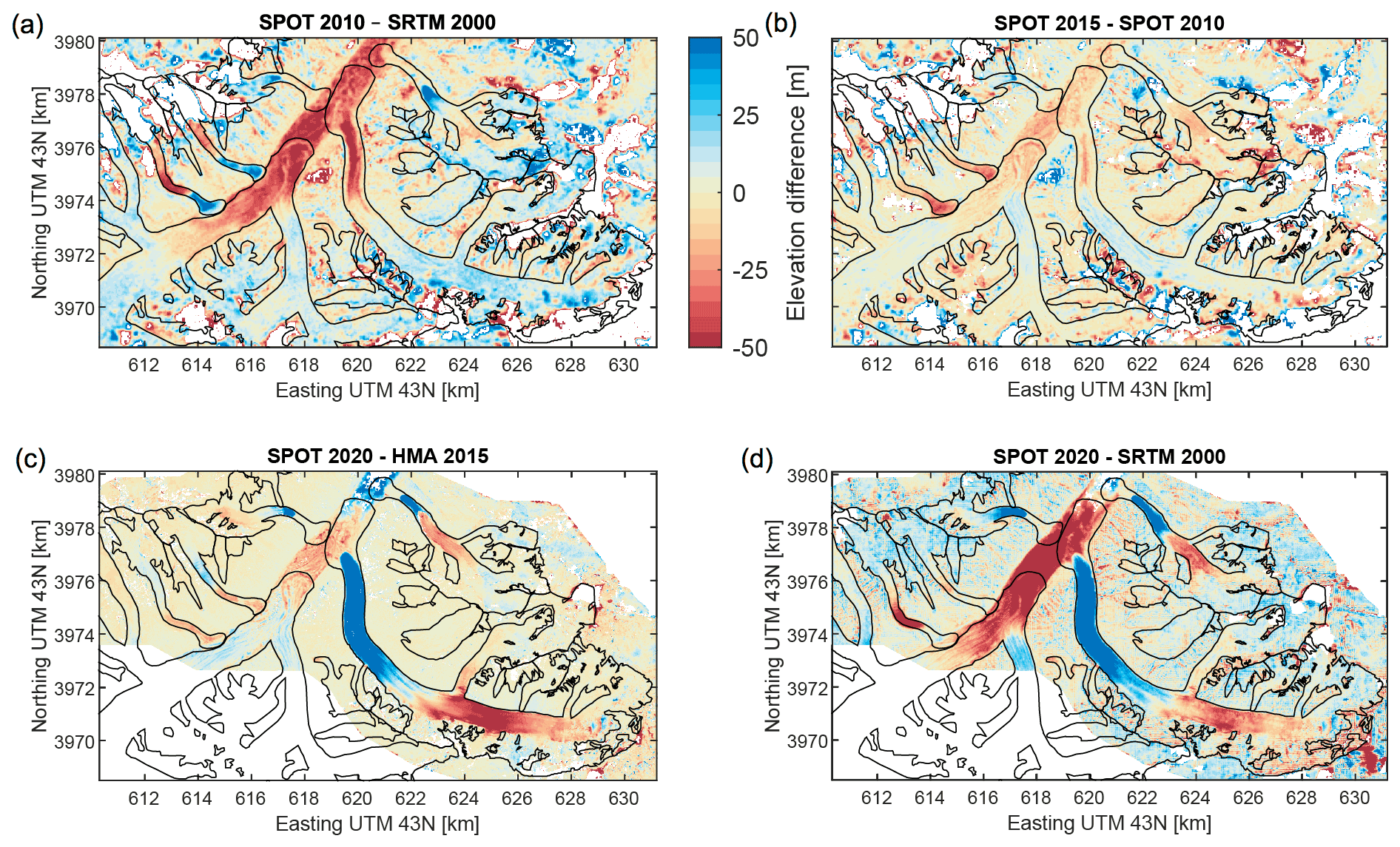
Figure 11 Two-dimensional elevation difference maps over the study region. (a) SPOT 2010 − SRTM 2000, (b) SPOT 2015 − SPOT 2010, (c) SPOT 2020 − HMA 2015, (d) SPOT 2020 − SRTM 2000. A comparison between the SPOT 2015 and the HMA DEM from 2015 is shown in Fig. S13.

5.5 Uncertainty assessment

5.5.1 Glacier length changes

Uncertainties in the length changes are estimated to be on the order of 1 image pixel, i.e. 60 m for MSS, 30 m for TM, 15 m for OLI pan and 10 m for Sentinel-2. As frontal advances have only been measured for a change of at least 3 to 4 pixels, the given values should be well outside the uncertainty range in most cases. However, the calculated frontal advance rates for glacier NN9 and North Chongtar (Fig. 4b) show fluctuations. These can be attributed to the measurement uncertainties so that in reality the increase might have been smoother and more gradual. There is thus some caution to not overinterpret the details of the change rates.

5.5.2 Flow velocities

The displacements measured by Landsat over the selected stable areas show median values close to the expected value of 0 m d⁻¹, with a MAD between 0.01 and 0.04 m d⁻¹, as reported in Table S2. Among the Landsat data, Landsat 7 shows the smallest standard deviation based on the MAD. For Sentinel-2, the uncertainties in the displacement on stable terrain are lower for the pairs with a time interval of approximately a year. For these pairs, the median and the MAD of the velocity are of the same order of magnitude as the Landsat results. For shorter time intervals (5 to 45 d), the Sentinel-2 velocity shows medians between 0.15 and 1.58 m d⁻¹, with a maximum MAD of 1.39 m d⁻¹. Displacement from Planet data gives a larger error with medians and MAD values ranging from 0.3 to 2.50 m d⁻¹. One pair showed a significantly higher error, with a median value of 8.64 m d⁻¹ and a corresponding MAD value of 4.76 m d⁻¹, which is of a similar order of magnitude to the displacement measured in the centreline of the glacier (13.89 m d⁻¹). TSX revealed the lowest uncertainty, with values of both median and MAD close to 0 m d⁻¹.

5.5.3 Elevation data

The median elevation differences on stable bedrock to the reference DEM (HMA DEM) are 1.02 m (SRTM), 1.03 m (SPOT 2010), −0.12 m (SPOT 2015) and 1.08 m (SPOT 2020), with standard deviations of 3–15 m (Table S3). Also mean elevation differences, which are more sensitive to extreme values, are < 1.4 m for all DEM difference pairs except for the SPOT 2020–SRTM2000 DEM pair (2.4 ± 8.8 m). These are small differences and fully within the range of expected uncertainties (after successful co-registration), considering the very steep and rugged terrain. We found no indication of remaining horizontal shifts between the DEMs (this would be visible as an aspect-dependent pattern in Fig. 11). The comparison of the SPOT 2015 and HMA 2015 DEM (Fig. S13) shows a minor tiling effect caused by the composite nature of the HMA DEM in the upper accumulation areas of North and South Chongtar. The mean uncertainty in the ATL06 ICESat-2 data was ±5.37 m. However, we assume that ATL03 elevation uncertainties are on the order of decimetres on the relatively smooth glacier surface.

5.6 Sensor inter-comparison

5.6.1 Velocities

As can be seen in Fig. 7a, velocity values derived from the (optical) 15 m resolution Landsat 8 panchromatic band for the period July 2018 to July 2019 are about the same as from (also optical) 10 m resolution Sentinel-2 data for the period August 2018 to August 2019. Both lines are basically on top of each other. The same applies to the Landsat 8 velocities for the period September 2016 to October 2017 compared to Sentinel-2 values over the period November 2016 to November 2017. The velocities derived from the (SAR) TSX sensor over the short period April to May 2014 also compare well with the annual mean values from Landsat 8 over the period July 2013 to July 2014. In Fig. S9 we show the related velocity differences with respect to the distance along the centreline for all three comparisons, revealing that they are largely within ±0.03 m d⁻¹ for the region between km 9 and the terminus. They are therefore as small as the stable-terrain uncertainties listed in Table S2. Between km 0 and 9 only a few values are available for the optical sensors, and these are subject to outliers. The differences are thus higher but in most cases still smaller than the flow velocity.

The (optical) Planet CubeSat images cover only the lower part of the glacier. Here, the Planet velocity (Fig. S10) reveals the same increase–decrease pattern as the Sentinel-2 velocity profile (Fig. 7b). Direct comparison of the flow velocities reveals much larger differences, but compared to the much higher flow velocities still only small differences (Fig. S11). These can be related to slightly different time intervals and the rapidly changing crevasse pattern at high flow velocities. On the other hand, the differences are large when comparing velocities derived from Sentinel-1 (SAR) with the optical Sentinel-2 (Fig. S12). The large image template sizes of 128×64 (450 m × 900 m) for South Chongtar (tongue width 800 m) result in a strong underestimation of Sentinel-1 velocities, with errors much greater than those reported in previous studies for larger Arctic glaciers (Paul et al., 2017a; Strozzi et al., 2017). The information density is also very low compared to Sentinel-2, indicating that Sentinel-1 data do not reveal sufficient detail about the surge.

5.6.2 Elevation changes

Of the seven analysed elevation datasets, ICESat-2 elevation profiles show most detail compared to the DEMs and are also resolving small surface features such as crevasses and seracs (Fig. S6). Both the weak and the strong laser beams of ICESat-2's three beam pairs provide equally good data in the snow-covered accumulation areas (Fig. S6a and b). On darker and more rugged surfaces the weak beam yields considerably fewer photon returns than the strong beam (bottom panels in Fig. S6e and f).

Elevation differences between the HMA DEM and the SPOT DEM from 2015 are depicted in Fig. S13. A small advance of North Chongtar and a slight elevation increase on South Chongtar within the few months' time gap are visible. The latter is confirmed by the cross-transects in Fig. S6c and d. In contrast, the elevations of the two 2015 DEMs agree very well for the transects in the upper accumulation area (top panels) and the down-wasting tongue in the main valley (bottom panels). Apart from artefacts and local differences in very steep terrain, elevations of the DEMs from 2015 agree very well both on and off glaciers.

The elevation changes derived from the ASTER DEM time series by Hugonnet et al. (2021) shown in Fig. S14 are similar to the time series we analysed from SRTM, SPOT and the HMA DEMs (Fig. 11). The ASTER DEMs have more artefacts and local differences, in particular in very steep terrain. In contrast, the strong spatial filtering inherent in the ASTER dataset smoothens artefacts and data gaps off and to some degree also details on glaciers. Locally, the ASTER dataset is less complete; e.g. the advance of North Chongtar is not well covered, and the advance of the glacier NN8 is not visible.

There are no further insights when splitting the 2000–2010 period into a 2000–2004 and 2005–2009 period, but the 2000–2019 period from ASTER (Fig. S14f) reveals the up to 40 m elevation increase in the upper region of South Chongtar. This “reservoir zone” seemingly stretches over the entire upper glacier rather than being an isolated region. In 2019 the surge had not started, so the strong elevation loss in its lower part from post-surge down-wasting of the previous surge is also very prominent. Elevation gain from 2000 to 2019 is also visible for the upper part of Sarpo Laggo Glacier and the lower part of Moni Glacier.

6 Discussion

6.1 Interpretation of the surges

The contrasting surge behaviour of North and South Chongtar glacier is remarkable in that the two glaciers with probably the highest (South Chongtar) and lowest (North Chongtar) flow velocities and advance rates during a surge (in the entire Karakoram) can be found side by side. At first glance, it seems that the sudden, short-lived surge of South Chongtar is hydrologically controlled (Alaska type), whereas the neighbouring North Chongtar surge seems thermally controlled (Svalbard type). However, as Quincey et al. (2015) noted, this simplified picture does not work well for many glacier surges in the Karakoram, which often show characteristics of both types. For example, the South Chongtar surge reached its maximum flow velocities in summer rather than winter, and its drop is very slow rather than fast. For a hydrologically controlled surge one would expect a surge start in winter (when efficient basal hydrology switches to inefficient) and a sudden end of the surge in summer (when basal water can again be released efficiently) (e.g. Kamb et al., 1985; Raymond, 1987; Sharp, 1988). Moreover, flow velocities increased slowly, steadily and over large parts of the glacier rather than being located at a clearly localized surge front. These observations fit better with a thermally controlled surge (e.g. Fowler et al., 2001) and imply that both mechanisms apply, and the surge mechanism could be named “hybrid”.

The slow and near-constant advance of North Chongtar and NN9 might not even be classified as a surge, but given that both glaciers also developed nearly all characteristics of a surge at some point (e.g. a heavily crevassed surface, shear margins, strong increase in flow velocity, high frontal advance rates, mass transfer from a reservoir to a receiving zone), the former advance phase might be seen as a part of the surge. Still, from the evolution of advance rates or flow velocities alone it is nearly impossible to pin down the exact surge onset for North Chongtar. Morphological changes (heavy crevassing, shear margins) indicate that this might have happened around 2010, but considering the near-linear increase in advance rates after 1996, one might assign the onset also to that year. In any case, the more or less constant advance for more than 30 years before 1996 is exceptional and only comparable to the very slow advance of Maedan Glacier in the neighbouring Panmah region that also started in the 1960s, before advance rates considerably increased in the mid-1990s, and the glacier started surging (Bhambri et al., 2017; Paul, 2020). Such prolonged advances might also be a consequence of a positive mass balance that one glacier converted to a continuous advance and another one to a surge (Lv et al., 2020). At least the elevation change pattern of North Chongtar over the 2000–2020 period reveals a clear and typical redistribution of mass from a higher reservoir zone to a lower receiving zone.

This is different for NN9, which only shows elevation increase in its lower part over this period without any measurable surface lowering higher up. This rather unique criterion for surge identification fails here and would exclude the glacier from being of surge type. However, a different impression emerges when looking at the temporal evolution of advance rates and flow velocities. In 2016 the former increased considerably from about 40 m yr⁻¹ to more than 1 km yr⁻¹, and the morphology of the surface changed from rather smooth to highly crevassed. Measurable flow velocities increased in 2019 from 0.2 to 0.8 m yr⁻¹, and the Landsat 8 image pair from 2018 to 2019 (Fig. 5d) also reveals an increase. With its recent rapid advance, the glacier has now reached its former 1971 maximum extent and also looks the same in terms of a completely crevassed surface (Paul, 2020). The slow advance might have resulted from a positive mass balance but could also be a thermally controlled surge. However, the recent increase in advance rates could also be due to a hydrologically controlled surge and/or due to the steep slope and dynamic effects. Compared to North Chongtar, the switch from advance to surge occurred much more sudden.

For South Chongtar the situation is clearer as its rapid advance and more than 100-fold increase in flow velocities (from 0.2 to more than 25 m d⁻¹) are typical for a hydrologically controlled surge with increasing basal water pressure. We assume that its thin lowest part was frozen to the bed (e.g. Obu et al., 2019), effectively blocking water release for some time. The interesting points of the current surge are (a) the gradual increase in flow velocities in the region above its fixed terminus (at km 13.5), (b) the extreme velocity increase from July to September 2020, (c) the high maximum velocities of 30 m d⁻¹, (d) the location of the maximum away from the centreline, and (e) the more or less constantly high flow velocities over large parts of its length from January to May 2021. The latter is responsible for the ongoing mass transport and advance of the terminus and implies that basically the entire glacier was activated by the surge. As mentioned above, points (a) and (e) are more typical for thermally controlled surges, so with both characteristics this surge can be classified as hybrid. That velocities increase from the centre to the boundary of a glacier (Fig. 9) is likely rather unique. We assume this is caused by the surrounding topography, i.e. the change in flow direction from north-west to north imposed by the mountain walls. The centre of the advancing terminus collided with the southern rock wall and was then diverted to a different direction. As the glacier was likely sliding over its full width, the resistance at the boundaries was likely limited.

Maximum surface flow velocities of 30 m d⁻¹ are only visible with Planet, and to the edge of the glacier (Fig. 9), Sentinel-2 values peak at 27 m d⁻¹. This is likely due to the higher resolution of Planet compared to Sentinel-2 and hence to the smaller region used for spatial averaging. Also the shorter time period considered (3 d) might play a role. Whereas high flow velocities of about 15 m d⁻¹ have been reported previously (Quincey et al., 2015; Paul et al., 2017b; Bhambri et al., 2020), values above 25 m d⁻¹ are only rarely observed in the Karakoram (Rashid et al., 2020). The latter study reports values near 50 m d⁻¹ for the last surge of Shispar Glacier (derived from 3 m Planet data), but the flow fields look a bit “bumpy”, and image processing artefacts might have contributed to the high values. We assume that the rapid increase in flow velocities during July and August was due to additional lubrication from summer surface meltwater.

In principle, a surge simply moves mass downstream, implying that the net volume change should be about zero. However, if surges take place over very long periods (> 5 years) there will also be a signal from the usual ablation and accumulation. Moreover, for DEMs derived from optical sensors, problems in snow-covered or steep terrain (shadow) exist that might create data gaps in the region where the mass has been removed (or where mass gain took place before a surge). Both effects can create biases, leading to over- or underestimation of calculated volume changes. These apply also to the changes calculated over 10-year periods and the SPOT DEM from 2010 that had data voids in the steep upper regions of some glaciers. As a consequence, volume changes calculated with this DEM are incomplete and need to be interpreted with care. However, as both positive and negative changes take place in regions of increased uncertainty, the net effect is likely small.

6.2 Uncertainties

The 1-pixel uncertainty in deriving terminus positions and length changes translates into an uncertainty in the calculated advance rates. How large the uncertainties are depends on the sensor resolution and the time period between two measurements. It is assumed that at least a part of the short-term variations in the advance rates of NN9 and North Chongtar are due to these uncertainties rather than real variability.

With the exception of the Planet data, the uncertainty in the velocity measured over stable terrain by all sensors is 1 or 2 orders of magnitude smaller than the maximum displacement observed on the glacier along the centreline, even for the two small glaciers NN9 and North Chongtar. For them, cloud cover has been identified as a major challenge for optical sensors. In fact, the selection of the satellite pairs prioritized the reduction in cloud cover on South Chongtar rather than NN9 and North Chongtar, which were rarely cloud-free. Hence, it is not only spatial resolution that is responsible for data limitations.

In general, the uncertainties in glacier flow velocity measurements are mainly related to co-registration accuracy, orthorectification, the time interval between image pairs, surface conditions (shadow, snow, etc.) and the spatial resolution of the images. The larger the time window between two pairs, the smaller the uncertainty in the measured velocity. Despite the higher resolution, the uncertainty is higher for Planet than for Sentinel-2. For Sentinel-2, the orthorectification error is minimized because the imagery comes from the same relative orbit (Kääb et al., 2016). In contrast, we have different orbital paths between Planet image pairs, and therefore further geometric corrections may be needed to minimize this error, as also suggested by Kääb et al. (2017) and Millan et al. (2019). Also the very small stable-terrain uncertainties in TSX are likely due to the accurate co-registration of the image pairs. The observed elevation changes exceed the DEM elevation uncertainties by an order of magnitude or more, which makes our elevation change analyses very robust. For volume change studies, data gaps in the DEMs and remaining blunders and bias from clouds or other sources cause greater uncertainties than the elevation uncertainties themselves (McNabb et al., 2019). Data gaps occur, however, mostly in the accumulation areas due to reduced contrast over snow, more persistent cloud cover and steeper terrain. Moreover, surface elevation tends to change much less here than is the case for the tongues, and uncertainties might become as large as the changes. The elevation accuracy of the ICESat-2 ATL03 product is clearly superior to all DEMs analysed within this study.

6.3 Sensor capabilities and limits

The sensor inter-comparison revealed a very good agreement between the velocity data derived from both TSX StripMap mode and Sentinel-2 with Landsat 8 (Fig. 7a), as well as between Sentinel-2 and Planet (Fig. S11). This confirms that all three optical sensors can be used to derive the temporal evolution of flow velocities – cloud cover, snow conditions and cast shadow permitting. The key point is the choice of the temporal baseline of image pairs as a function of glacier surface changes, sensor resolution and the targeted velocity field. At 20 m d⁻¹ a 5 d interval is equivalent to a change by 10 pixels with Sentinel-2 and 20 pixels with Planet over 3 d (assuming a 3 m resolution). At 0.1 m d⁻¹ the displacement is about 35 m (3 Sentinel-2 pixels) after a year, which is at the lower end of what is detectable with offset-tracking.

For SAR data the typical limitations are layover and foreshortening, radar shadow, SAR penetration, and decorrelation. Actually, none of these created problems for the TSX and Sentinel-1 image pairs used here. However, Sentinel-1 performed poorly even on the largest glacier, South Chongtar. This was mostly due to the fact that this glacier has a long and narrow tongue (width less than 800 m) situated between steep mountain flanks. Because of the relatively large size needed for the matching window (Fig. S4), too many non-moving off-glacier pixels are included, affecting the velocity retrieval considerably (Fig. S12). Also, the large and fast surface changes on the rapidly surging glacier might have changed the backscatter patterns too much to be tracked over time (Strozzi et al., 2017). The minimum width of a glacier to be reliably monitored with Sentinel-1 in the Himalayas is likely around 2 km. In contrast, TSX yielded dense and consistent velocity values for all three glaciers (pre-surge phase). As it seems, the map in Fig. 5b nicely captures the flow acceleration of North Chongtar in 2012, which decreased afterwards (Fig. 6b). The much noisier values from Landsat 8 in this figure (compared to Sentinel-2 and TSX) revealed that the 15 m resolution of the Landsat panchromatic band is seemingly insufficient to track displacements precisely. Note, though, that these comparisons are not strict as the sensors have different resolutions, and the datasets cover different phases of the surges and thus different surface conditions.

The compared DEMs are of similar quality over glaciers, but the SPOT 2010 DEM used by Gardelle et al. (2013) suffered from strong artefacts at steep slopes. The elevation values of the SPOT 2015 and HMA DEM (which is also from 2015 in this region) are basically identical apart from individual raster cells (e.g. showing the advancing terminus of North Chongtar). So elevation changes from 2000 (SRTM) to 2015 (HMA DEM) can also be derived from freely available DEMs. The SPOT 2020 DEM is of superb quality, but the raw image pair had to be purchased. For a study looking at specific glaciers this is certainly worthwhile but does typically prevent larger regions from being covered.

The surface elevation detail and accuracy of the freely available ICESat-2 ATL03 photon data surpass all other datasets, including the SPOT 2020 DEM (Fig. S6). When combined with one or several DEMs, the higher temporal resolution provides additional information on how the elevation changed in between DEM time stamps. This may be very useful for slower changes or to further constrain the onset and end of a rapid change, such as a surge. However, ICESat-2 only provides elevation profiles with varying locations, which makes this data type more demanding to analyse. The footprints of the ICESat-2 ATL06 time series alone are too sparse to derive any useful trends in glacier surface elevation.

The DEM time series from ASTER images (Fig. S14) derived by Hugonnet et al. (2021) shows the same trends as from the DEMs used here. They provide further information over the 2000–2005 and 2005–2010 periods but miss the surge of South Chongtar as they end in 2019. On the other hand, they cover a much larger area and clearly reveal the increase in surface elevation of South Chongtar over the full 2000–2019 period. The coverage of the smaller glaciers is noisier with ASTER than with the DEMs we have used, and locally values are missing, but the temporal evolution over several larger glaciers can be well followed. Deriving further DEMs from future ASTER stereo scenes might thus help to determine total volume changes after all surges have come to an end, including the not yet visible volume loss in the reservoir zone of NN9.

7 Conclusions

We identify and present an analysis of three glacier surges in the central Karakoram, all taking place in the same small region but with very different characteristics and possibly forcing mechanisms. South Chongtar showed advance rates of more than 10 km yr⁻¹, velocities up to 30 m d⁻¹, and surface elevations increasing by 170 m, all within a surge duration of about 2–3 years. The 3-times-smaller and neighbouring North Chongtar Glacier had a slow and almost-linear increase in advance rates (up to 500 m yr⁻¹) over a period of almost 50 years, flow velocities below 1 m d⁻¹, and elevation increases of up to 100 m. A more active phase from 2010 to 2015 was followed by a continuation of its slow advance. The even smaller glacier NN9 changed from a slow advance to a full surge within a year, reaching advance rates higher than 1 km yr⁻¹ but showing the typical surface lowering higher up only recently. Total length changes reached between 2 and 2.7 km for the three glaciers, and the size of NN9 changed by more than 20 %. For South Chongtar, maximum flow velocities are found near its southern boundary rather than in the centre.

At first glance, the surge of South Chongtar clearly resembles the classical Alaska-type surge (hydrologically controlled), whereas North Chongtar and NN9 better fit to the Svalbard type (thermally controlled). However, the summer onset and slow velocity decay of the South Chongtar surge and the sudden change in frontal advance rates of NN9 hint at the respective other type, resulting in a change in characteristics. North Chongtar has not changed type, but surge onset is difficult to determine as advance rates increased linearly, morphological changes developed slowly, and a 50-year advance might also be called a surge. If the definition of a surge were stricter, we would assign the surge onset of NN9 and North and South Chongtar to 2017, 2005–2010 and August 2019, respectively. We speculate that the thin, lower part of South Chongtar was cold ice frozen to the bed, reducing possibilities for the terminus to advance and causing basal pressure to strongly increase.

The sensor inter-comparison revealed that Landsat 8 and Sentinel-2 are difficult to be used jointly for determination of geometric changes as their geolocation differs (> 30 m). Flow velocities agreed well across sensors for South Chongtar, except for Sentinel-1, which had problems due to its narrow tongue (800 m). However, the backscatter intensity images provided a time series of surge evolution at a near-constant interval that is undisturbed by clouds. At the two smaller glaciers NN9 and North Chongtar, the optical sensors still provided reasonable and consistent flow velocities, but limits due to spatial resolution and cloud cover became visible (more noise). The TerraSAR-X acquisitions in StripMap mode revealed by far the best results and depicted the surge of North Chongtar accurately.

After proper co-registration, all DEMs provided useful results to track elevation and volume changes, independent of glacier size. The two SPOT DEMs from 2010 and 2015 suffered from artefacts at steep slopes, but the latter compared very well to the HMA DEM. The high-resolution SPOT6 DEM from October 2020 had impressive quality and allowed an accurate calculation of the volume change in all glaciers up to this point in time. The very precise ICESat-2 elevation profiles provided additional information in space (glacier surface details) and time (between the DEMs) that matched well to the other datasets. The ASTER DEM time series missed detecting local changes in smaller glaciers but provided a larger overview and complementary information on cumulative elevation changes shortly before the surge of South Chongtar started.

All three glaciers are still advancing, and South Chongtar and NN9 are now colliding. The bulldozing of the South Chongtar terminus into the down-wasting ice of Sarpo Laggo Glacier is already creating interesting morphological changes. North Chongtar might again reach the floor of the main valley as in the 1930s, but this could take some more years. We conclude that the past and further evolution of these and other glacier surges can be well observed from satellite data, at best by combing all available datasets.