Simulating the Holocene deglaciation across a marine-terminating portion of southwestern Greenland in response to marine and atmospheric forcings

Numerical simulations of the Greenland Ice Sheet (GrIS) over geologic timescales can greatly improve our knowledge of the critical factors driving GrIS demise during climatically warm periods, which has clear relevance for better predicting GrIS behavior over the upcoming centuries. To assess the fidelity of these modeling efforts, however, observational constraints of past ice sheet change are needed. Across southwestern Greenland, geologic records detail Holocene ice retreat across both terrestrial-based and marine-terminating environments, providing an ideal opportunity to rigorously benchmark model simulations against geologic reconstructions of ice sheet change. Here, we present regional ice sheet modeling results using the Ice-sheet and Sea-level System Model (ISSM) of Holocene ice sheet history across an extensive fjord region in southwestern Greenland covering the landscape around the Kangiata Nunaata Sermia (KNS) glacier and extending outward along the 200 km Nuup Kangerula (Godthåbsfjord). Our simulations, forced by reconstructions of Holocene climate and recently implemented calving laws, assess the sensitivity of ice retreat across the KNS region to atmospheric and oceanic forcing. Our simulations reveal that the geologically reconstructed ice retreat across the terrestrial landscape in the study area was likely driven by fluctuations in surface mass balance in response to Early Holocene warming – and was likely not influenced significantly by the response of adjacent outlet glaciers to calving and ocean-induced melting. The impact of ice calving within fjords, however, plays a significant role by enhancing ice discharge at the terminus, leading to interior thinning up to the ice divide that is consistent with reconstructed magnitudes of Early Holocene ice thinning. Our results, benchmarked against geologic constraints of past ice-margin change, suggest that while calving did not strongly influence Holocene ice-margin migration across terrestrial portions of the KNS forefield, it strongly impacted regional mass loss. While these results imply that the implementation and resolution of ice calving in paleo-ice-flow models is important towards making more robust estimations of past ice mass change, they also illustrate the importance these processes have on contemporary and future long-term ice mass change across similar fjord-dominated regions of the GrIS.

1 Introduction

Over the past few decades, the Greenland Ice Sheet (GrIS) has experienced accelerating ice mass loss driven by increases in surface melt, runoff, and dynamic ice loss at marine-terminating margins (IMBIE, 2019). While projected mass loss from the GrIS is expected to be driven increasingly by its surface mass balance (SMB; Enderlin et al., 2014; Vizcaino et al., 2014; Goelzer et al., 2020) and attendant meltwater runoff (Fettweis et al., 2008; Lenaerts et al., 2019), considerable uncertainty exists regarding how oceanic forcing will influence GrIS mass loss, particularly through ice calving processes (Goelzer et al., 2020; Choi et al., 2021). The satellite-based observational record of GrIS change only spans a few decades, making it difficult to identify and disentangle the key drivers of GrIS mass change, as well as to understand over which timescales they operate. Fortunately, geologic records detailing the retreat history of the GrIS provide an important metric for evaluating numerical ice sheet models and help pinpoint the contributions of various driving mechanisms to GrIS change. When combined, numerical ice sheet models and geologic reconstructions can provide key insights into GrIS behavior in a warming climate across centennial to millennial timescales.

The current interglacial, the Holocene (the last 11.7 kyr), is characterized by prolonged warmth with proxy records suggesting that temperatures during the Early to Middle Holocene were 3±1 ^∘C warmer than the pre-industrial period (Briner et al., 2016; Lecavalier et al., 2017), which drove widespread retreat of the GrIS margin at a rate of ice mass loss exceeding 20th century values (1900–2000 CE; Young and Briner, 2015; Briner et al., 2020). Across southwestern Greenland, a detailed geologic record of Holocene ice-margin retreat encompassing both terrestrial and marine-terminating environments exists, providing an ideal test bed for ice sheet models to test the sensitivity of past ice-margin migration to atmospheric and marine forcings (Larsen et al., 2014; Lesnek et al., 2020; Young et al., 2020, 2021). Where land-based ice existed, well-dated moraine sequences constrain ∼120 km of ice retreat from the present-day coastline to just outboard of the present-day ice margin (Lesnek et al., 2020; Young et al., 2020) and have been shown by ice sheet models to be driven by negative SMB in response to Early Holocene warming (Cuzzone et al., 2019; Downs et al., 2020; Briner et al., 2020).

Unlike the land-based portions of southwestern Greenland, however, across the marine-based region covering the forefield around Kangiata Nunaata Sermia (KNS; Fig. 1), it remains unknown what drove this rapid ice-margin retreat during the Early Holocene (Young et al., 2021). While links between atmospheric warming and runoff-induced terminus retreat have been implicated as reasons for the most recent historical retreat across the KNS region (Lea et al., 2014a, b), the longer-term triggers of rapid Holocene ice retreat are not constrained by the geologic data alone. Because of the well-dated chronology detailing Holocene ice retreat across this region, however, ice sheet models are well poised to address questions surrounding the scales of influence atmospheric and oceanic forcings play on long-term ice-margin and mass change. However, as many paleo-ice-flow models employ model grids that are relatively coarse (10 km or greater), ice-margin migration and ultimately ice discharge through fjord systems may be poorly simulated or not captured as many models cannot resolve the complex and narrow fjord geometries found across the GrIS (Cuzzone et al., 2019).

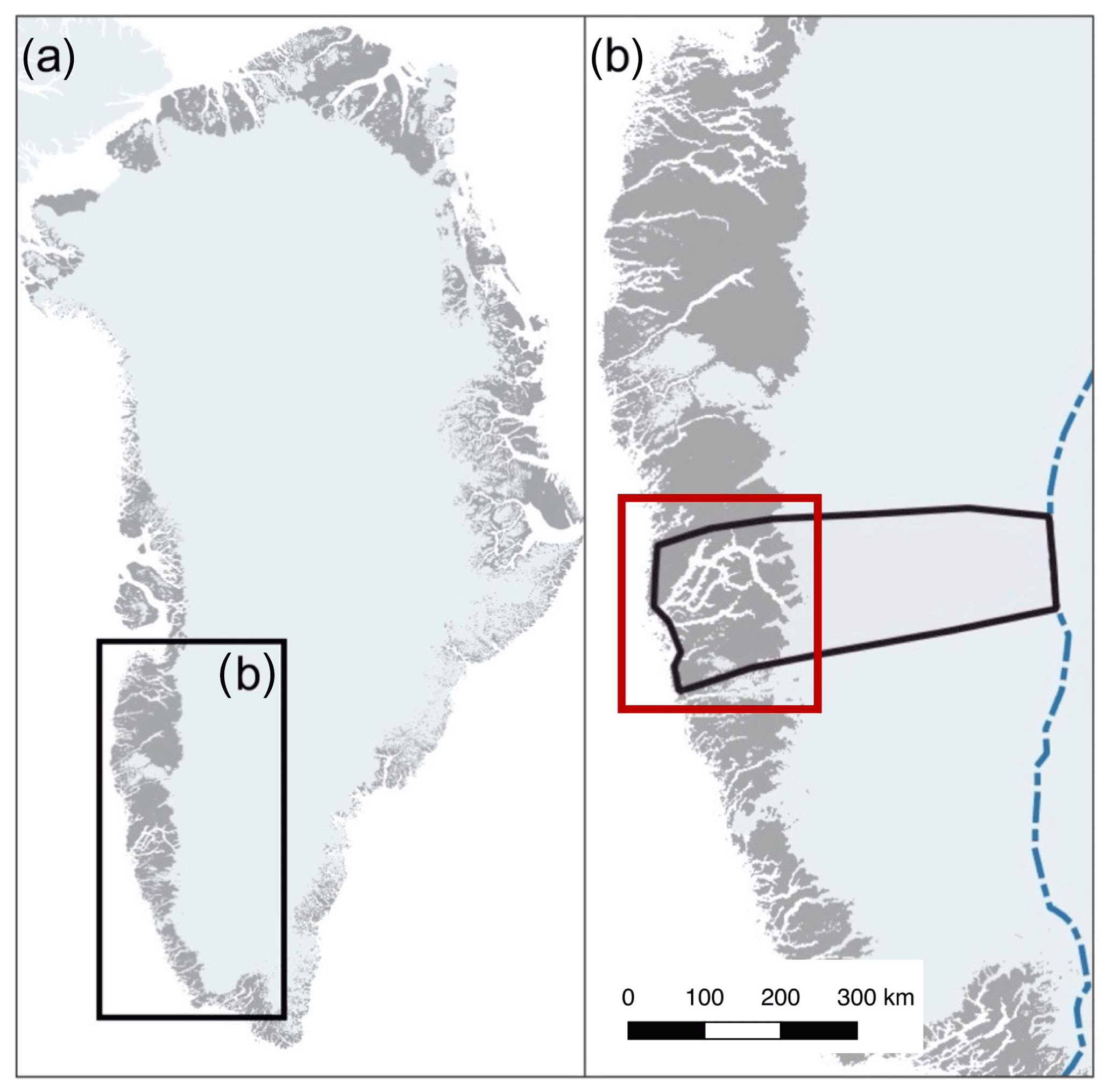
Figure 1 (a) The Greenland Ice Sheet. Highlighted is southwestern Greenland, where the ice model domain resides. (b) Southwestern Greenland. The ice model domain is outlined (bold black line), extending between the present-day coastline and ice divide (dashed blue line; Rignot and Mouginot, 2012). The red box corresponds to the area in Figs. 5, 6, and 8.

Building on recent advances in calving front dynamics in the Ice-sheet and Sea-level System Model (ISSM; Larour et al., 2012), we use a high-resolution regional ice sheet model to investigate the Holocene ice retreat across the KNS forefield. Our simulations build on prior ice modeling efforts across southwestern Greenland that were driven by novel reconstructions of past climate (Badgeley et al., 2020; Briner et al., 2020). While our past ice flow modeling efforts excluded ice–ocean interactions (Briner et al., 2020), our simulations presented here take advantage of the recent implementation of physically based calving schemes in ISSM to specifically address how Holocene ice retreat across the KNS forefield was influenced by marine and atmospheric forcings. Moreover, this work provides a foundation for future experiments using ISSM to simulate the influence of ice–ocean interactions on the Holocene variability in the broader GrIS.

2 Holocene ice retreat across the KNS forefield

Decades of radiocarbon dating and, more recently, cosmogenic ¹⁰Be dating track the retreat of the GrIS in the KNS region through the Holocene (Weidick et al., 2012, and references therein; Larsen et al., 2014; Young et al., 2021). Minimum-limiting radiocarbon ages from the outer coast near Nuuk range from ca. 11.2 to 10.6 ka, which is mimicked by ¹⁰Be ages of ca. 10.7 and 10.4 ka (Fig. 2). Between the outer coast and the modern GrIS margin at KNS are numerous radiocarbon and ¹⁰Be ages that are largely indistinguishable and require rapid deglaciation of the region spanning about a millennium (Weidick et al., 2012; Larsen et al., 2014; Young et al., 2021). Perhaps most relevant here are ¹⁰Be ages in the immediate KNS region from just beyond the historical ice limit that suggest KNS had retreated within or near its current position by ca. 10.3 ka (Young et al., 2021). Radiocarbon ages from raised marine deposits, which require ice-free conditions, adjacent to the main KNS fjord appear slightly younger than regional ¹⁰Be ages. These radiocarbon ages, however, are minimum-limiting ages, and an up-fjord radiocarbon age of ca. 10.2 ka from a bivalve reworked by a KNS readvance requires that the main fjord deglaciated prior to ca. 10.2 ka (Fig. 2). Collectively, the radiocarbon and ¹⁰Be ages suggest rapid and synchronous deglaciation of both the landscape and fjord systems between the outer coast near Nuuk and the modern margin at KNS. Lastly, ¹⁰Be ages from slightly beyond the historical limit to the north and south of KNS are slightly younger, suggesting that these ice margins may have lagged behind ice retreat in the immediate KNS region (Fig. 2).

Figure 2 KNS region with geological constraints that track GrIS retreat in the Early Holocene. Radiocarbon ages (red circles) and ¹⁰Be ages (yellow circles) are from Weidick et al. (2012), Larsen et al. (2014), and Young et al. (2021). For figure clarity, we only show the mean deglaciation age at each site (see Young et al., 2021, for full site descriptions). Radiocarbon and ¹⁰Be across the immediate KNS region are similar and reveal that deglaciation of the coast occurred ca. 11.2–10.7 ka, and KNS had retreated near or within its modern extent by ca. 10.3 ka. Radiocarbon ages in white text and black background are from marine deposits and constrain the timing of retreat within the main fjord. The figure has been modified from Young et al. (2021).

3 Model description and setup

3.1 Ice sheet model

We rely on ISSM, a thermomechanical finite-element ice sheet model, to simulate the Holocene ice history across the KNS forefield, and we follow similar published model setups (Cuzzone et al., 2019; Briner et al., 2020). The higher-order approximation of Blatter (1995) and Pattyn (2003) is used to solve the momentum balance equations. Our model domain centers on the KNS and Godthåbsfjord forefield, extending from the present-day coastline, where geologic observations show ice resided at the end of the Younger Dryas (Larsen et al., 2014; Lesnek et al., 2020), to the present-day ice divide (Fig. 1b; Rignot and Mouginot, 2012). The northern and southern boundaries of our model domain are chosen to represent regions of minimal north–south across boundary flow based on Holocene ice sheet simulations of southwestern Greenland (Briner et al., 2020). Anisotropic mesh adaptation is used to create a non-uniform model mesh that varies based upon gradients in bedrock topography from BedMachine v3 (Morlighem et al., 2017). Because fjord width across our domain is often <5 km and high-resolution grids are necessary for capturing grounding line dynamics (1 km; Seroussi and Morlighem, 2018), the horizontal mesh resolution varies from 1 km in fjords and areas of high bedrock relief to 15 km where the bedrock relief is low (Fig. 3).

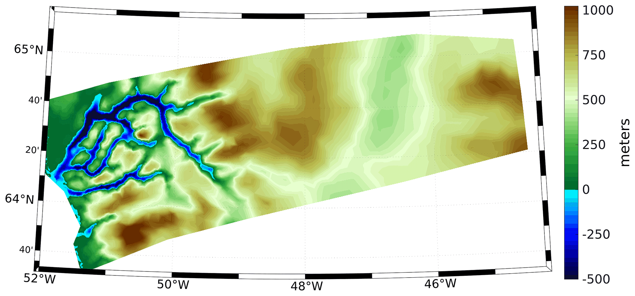
Figure 3 Bedrock topography for the model domain. Blue colors indicate areas that are below present-day sea level.

To capture the thermal evolution of the ice, our model uses an enthalpy formulation (Aschwanden et al., 2012) that captures both temperate and cold ice. We impose transient air temperatures at the surface and a constant but spatially varying geothermal heat flux at the base (Shapiro and Ritzwoller, 2004), and our model contains only five vertical layers in order to reduce computational load (Cuzzone et al., 2018, 2019). In order to capture sharp thermal gradients near the base and simulate the vertical distribution of temperature within the ice, we use quadratic finite elements (P1 × P2) along the z axis for the vertical interpolation following Cuzzone et al. (2018). This methodology has been successfully applied to simulate the transient behavior of the GrIS across geologic timescales and the contemporary period (Cuzzone et al., 2019; Briner et al., 2020; Smith-Johnsen et al., 2020).

We use a linear friction law, and, similar to Briner et al. (2020), we construct a spatially varying basal friction coefficient (k) under areas covered by the present-day ice sheet using inverse methods (Morlighem et al., 2010; Larour et al., 2012) that satisfies the best match between modeled and satellite-derived surface velocities (Rignot and Mouginot, 2012):

$$\begin{array}{}\text{(1)}& {\mathit{\tau }}_{\mathrm{b}}=-k^{\mathrm{2}}N{v}_{\mathrm{b}},\end{array}$$

where τ_b represents the basal stress, N represents the effective pressure, and v_b is the magnitude of the basal velocity. For contemporary ice-free areas, a spatially varying basal friction coefficient is constructed to be proportional to bedrock elevation following Åkesson et al. (2018):

$$\begin{array}{}\text{(2)}& k=\mathrm{100}\times {\displaystyle \frac{min\left[max(\mathrm{0},z_{\mathrm{b}}+\mathrm{800}),z_{\mathrm{b}}\right]}{max\left(z_{\mathrm{b}}\right)}},\end{array}$$

where z_b is the height of the bedrock with respect to sea level. For these parametrizations, the friction coefficient is low within fjords and is larger over areas of high topographic relief. This basal friction coefficient is allowed to vary through time based upon changes in the simulated basal temperature following Cuzzone et al. (2019). As simulated basal ice temperatures decrease with respect to present day, the friction coefficient will increase, and therefore sliding will decrease. The opposite occurs when simulated basal temperatures are warm relative to present day. Lastly, the ice rheology parameter B is temperature-dependent, following rate factors in Cuffey and Paterson (2010), and is initialized by solving for a present-day thermal steady state and allowed to vary during transient simulations (Cuzzone et al., 2018, 2019).

3.2 Ice-front migration and calving

We use the level-set method to track the motion of the ice front (Bondzio et al., 2016). The velocity of the moving ice front is calculated as follows:

$$\begin{array}{}\text{(3)}& {\mathit{v}}_f=\mathit{v}-(c+\dot{M})\mathit{n},\end{array}$$

where v_f is the ice velocity vector, v is the ice velocity vector at the ice front, c is the calving rate, $\dot{M}$ is the melting rate of the calving front, and n is the unit normal vector pointing horizontally outward from the calving front. For these simulations, we assume that the melting rate at the calving front is negligible compared to the calving rate.

To simulate calving, we rely on the physically based Von Mises stress calving (Morlighem et al., 2016), whereby the calving rate is related to tensile stresses within the ice:

$$\begin{array}{}\text{(4)}& c=\Vert v\Vert {\displaystyle \frac{\stackrel{\mathrm{̃}}{\mathit{\sigma }}}{{\mathit{\sigma }}_{\text{max}}}},\end{array}$$

where $\stackrel{\mathrm{̃}}{\mathit{\sigma }}$ is the von Mises tensile strength, $\Vert v\Vert$ is the magnitude of the horizontal ice velocity, and σ_max is the maximum stress threshold, which has separate values for grounded and floating ice. Under this formulation, the ice front will remain stable when $\stackrel{\mathrm{̃}}{\mathit{\sigma }}={\mathit{\sigma }}_{\text{max}}$, will retreat when $\stackrel{\mathrm{̃}}{\mathit{\sigma }}>{\mathit{\sigma }}_{\text{max}}$, and will advance when $\stackrel{\mathrm{̃}}{\mathit{\sigma }}<{\mathit{\sigma }}_{\text{max}}$. Tensile strength measurements of ice show a range of possible σ_max values, ranging between 150 and 3100 kPa (Petrovic, 2003). For this study we choose σ_max=600 kPa for grounded ice and 200 kPa for floating ice, which is within the ranges used by recent studies across Greenland (Bondzio et al., 2016; Morlighem et al., 2016; Choi et al., 2021).

3.3 Climate and surface mass balance reconstruction

We rely on a novel gridded paleoclimate reanalysis product that reconstructs the necessary climate variables of temperature and precipitation needed to calculate the surface mass balance history through the Holocene (Badgeley et al., 2020). Temperature was derived from oxygen-isotope records from eight ice cores, and five ice core accumulation records were used to reconstruct precipitation. This reanalysis relies on a data assimilation framework that combines the information from ice core proxies with climate-model simulations of the last deglaciation (Liu et al., 2009; He et al., 2013) to create a spatially complete (e.g., GrIS wide) and temporally consistent reconstruction of past temperature and precipitation. This reconstruction agrees well with independent proxies and previously published paleoclimate reconstructions (Badgeley et al., 2020). For new simulations presented here, we chose two end members of reconstructed precipitation and temperature from Badgeley et al. (2020). The high-temperature reconstruction was chosen, which has a greater magnitude of Early Holocene warming, as well as the low-temperature scenario, which has a more muted Early Holocene warming (Fig. 4a). Additionally, we choose the high- and low-precipitation scenarios (Fig. 4b), which differ in the magnitude and timing of peak Holocene precipitation. These reconstructions span a plausible range of temperature and precipitation scenarios as discussed in Badgeley et al. (2020).

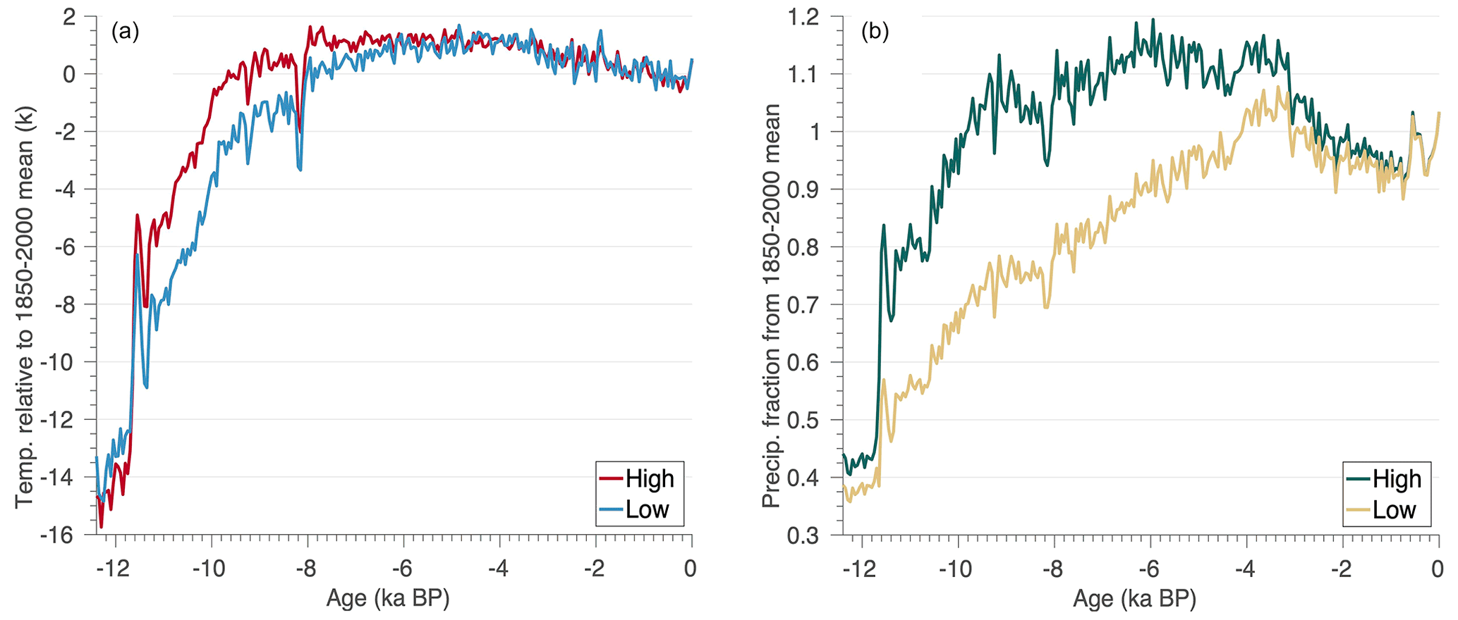
Figure 4 (a) Area-averaged (over model domain) mean annual temperature anomaly (k) relative to the 1850–2000 mean for the high- and low-temperature reconstructions from Badgeley et al. (2020). (b) Area-averaged (over model domain) mean annual precipitation as a fraction from the 1850–2000 mean for the high and low reconstructions from Badgeley et al. (2020).

The simulations discussed below use a combination of these forcings to address the possible role of varying climatic conditions. Following prior work (Cuzzone et al., 2019; Briner et al., 2020), we compute the surface mass balance over the Holocene using a positive degree day (PDD) method (Tarasov and Peltier, 1999; Le Morzadec et al., 2015). For this scheme, snow melts first at 4.3 $\mathrm{mm}{}^{\circ }{\mathrm{C}}^{-\mathrm{1}}{\mathrm{d}}^{-\mathrm{1}}$, and the remaining positive degree days are used to melt bare ice at 8.3 $\mathrm{mm}{}^{\circ }{\mathrm{C}}^{-\mathrm{1}}{\mathrm{d}}^{-\mathrm{1}}$. A lapse rate of 6 ${}^{\circ }\mathrm{C}{\mathrm{km}}^{-\mathrm{1}}$ is used to adjust the temperature of the climate forcings to ice surface elevation, while an allowance for the formation of superimposed ice is permitted following Janssens and Huybrechts (2000).

3.4 Experimental setup

For the reanalysis discussed in Sect. 3.3, temperature is expressed as anomalies from the 1850–2000 CE mean, and precipitation is expressed as a fraction of the 1850–2000 CE mean (Fig. 4). Following Briner et al. (2020), we apply these anomalies onto the 1850–2000 monthly mean climatology of temperature and precipitation from Box (2013) to produce the necessary Holocene temperature and precipitation forcings:

$$\begin{array}{}\text{(5)}& {\displaystyle }{T}_t={\stackrel{\mathrm{‾}}{T}}_{\text{(1850–2000)}}+\mathrm{\Delta }{T}_t,\text{(6)}& {\displaystyle }{P}_t={\stackrel{\mathrm{‾}}{P}}_{\text{(1850–2000)}}\times \mathrm{\Delta }{P}_t,\end{array}$$

where ${\stackrel{\mathrm{‾}}{T}}_{\text{(1850–2000)}}$ and ${\stackrel{\mathrm{‾}}{P}}_{\text{(1850–2000)}}$ are the monthly mean temperature and precipitation over 1850–2000 CE from Box et al. (2013), and ΔT_t and ΔP_t are the monthly anomalies from Badgeley et al. (2020). We perform four transient model simulations using four combinations of possible climate scenarios shown in Table 1. For each climate scenario, we run two simulations. First, simulations are performed in which the calving parameterization is turned on (denoted as “calving on”). Second, simulations are performed in which the calving parameterization is turned off (denoted as “calving off”). For these simulations, we apply a temporally constant melting rate under floating ice of 40 m yr⁻¹, which is consistent with contemporary melt rates derived near the grounding line of floating ice shelves across the GrIS (Wilson et al., 2017). We also perform additional simulations discussed further in Sect. 4.4 to assess sensitivity to the calving maximum stress thresholds and ocean-induced melt rates.

Table 1 Description of model experiments. See Fig. 4 for a display of the temperature and precipitation forcing scenarios.

We initialize our regional ice sheet model using present-day ice surface elevation from the Greenland Ice Mapping Project digital elevation model (Howat et al., 2014). A constant climate from 12 400 years ago is then applied for each experiment, allowing our model to reach equilibrium in ice volume and basal temperature, which takes 20 000 years. Since our simulations are regional in scale, we use boundary conditions of temperature, ice velocity, and thickness from a recent ice sheet simulation of west-southwest Greenland (Briner et al., 2020) and impose these as Dirichelt boundary conditions at the southern, northern, and ice-divide boundaries. The eastern boundary of our model domain extends outward to the present-day ice divide (Rignot and Mouginot, 2012), with the northern and southern boundary of our model domain extending to cover the KNS forefield. While the catchment for KNS may have changed during the Holocene and thus may have impacted ice flux into our domain, those changes are not constrained. Therefore, since we use consistent boundary conditions across our experiments, we consider that our results are primarily influenced by the surface climate and oceanic boundary conditions applied and not influenced by model domain extent. These boundary conditions are forced transiently throughout the Holocene simulations and use similar model setups and climate forcings as discussed here. Each model is then run transiently through time from 12 400 years ago to 1850 CE using the climatologies discussed above, and then from 1850 to 2013 we use monthly temperature and precipitation fields from Box et al. (2013). We use an adaptive time step, which varies between 0.02 and 0.1 years, depending on the Courant–Friedrichs–Lewy criterion (Courant et al., 1928). Discussed further in Sect. 5.3, we do not include glacial isostatic adjustment (GIA) in these simulations. Although GIA can influence the underlying bedrock topography and ultimately surface mass balance gradients and grounding line stability, changes during the Holocene across our domain are likely small (i.e., on the order of 100 m; Caron et al., 2018), and therefore we expect this to have a minimal impact on our simulated ice histories.

4 Results

We spin up each model as described above (Sect. 3.4) without the ice calving parametrization turned on. Only when we begin the transient simulation through the Holocene do we turn on the ice calving parametrization for the “calving on” scenarios (Table 1). Our transient simulations begin 12 400 years ago with the ice margin residing along the present-day coastline for all experiments, which is approximately consistent with where geologic constraints place the ice margin at that time (Young et al., 2021, and references therein).

4.1 Simulated deglaciation

First, we assess how our simulated deglaciation compares with geologic reconstructions of ice sheet change in the KNS region. Geological constraints outlined above reveal that ice retreated across the KNS forefield rapidly in the Early Holocene. While relatively little direct information exists detailing ice retreat within the fjords, the terrestrial portion of our domain (i.e., the inter-fjord bedrock landscape) became ice free between ∼11.2 and 9.5 ka as ice retreated from the modern coastline towards, and eventually surpassing, what is now the modern ice margin.

To compare against the geologic constraints, we determine when in time portions of our model domain become ice free (Fig. 5). Since ice can readvance over areas that had been deglaciated during our simulations, we take the youngest age at which locations in our simulations became ice free. Our simulations illustrate clear differences in the timing of deglaciation across terrestrial surfaces above sea level and within the fjords. For the high- and low-temperature scenarios, terrestrial surfaces deglaciate up to a few millennia earlier than the adjacent fjords. This difference in timing between the fjords and terrestrial surfaces is perhaps unsurprising given how fjord systems act as conduits draining the ice interior. This persistence of ice extent within the fjords despite elevated warming experienced during the Early to Middle Holocene illustrates the role of ice dynamics, which is explored further in Sect. 4.3.

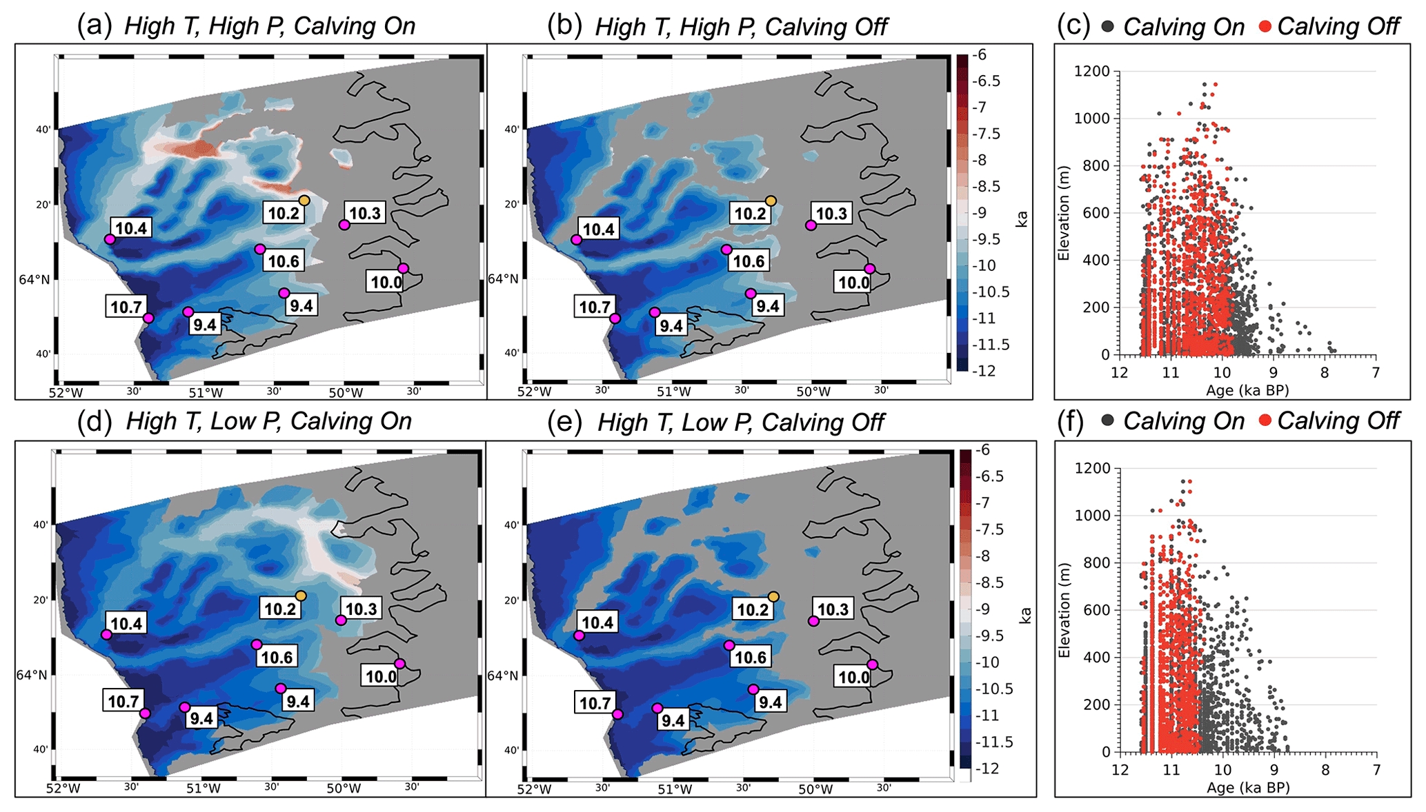
Figure 5 Map of simulated deglaciation ages for high-temperature scenarios with (a) high precipitation and calving on, (b) high precipitation and calving off, (d) low precipitation and calving on, and (e) low precipitation and calving off. Gray mask is the simulated ice extent at present day, and the black line denotes the actual present-day ice extent (Rignot and Mouginot, 2012). Magenta circles are the best estimate of the timing of deglaciation at that point based on ¹⁰Be surface exposure ages in thousands of years, and the yellow dot shows minimum limiting radiocarbon age (Young et al., 2021). Scatter plot of simulated deglaciation age (above sea level) versus bedrock elevation for (c) high temperature and high precipitation and (f) high temperature and low precipitation. Red dots are from simulations without calving, and black dots are for simulations with calving.

For the high- and low-temperature scenarios, there is little difference between the age of deglaciation on terrestrial surfaces for simulations that allow (Fig. 5a and b; Fig. 6a and b) and do not allow calving (Fig. 5d and e; Fig. 6d and e). In contrast, the deglaciation of terrestrial surfaces occurs later in the Holocene for the simulations using the high-precipitation scenario than for those simulations using the low-precipitation scenario. For simulations using the high-temperature scenario, these differences are up to 500 years (Fig. 5). For the low-temperature scenarios, terrestrial surfaces deglaciate up to 1000 years later for simulations using the high-precipitation forcing (Fig. 6).

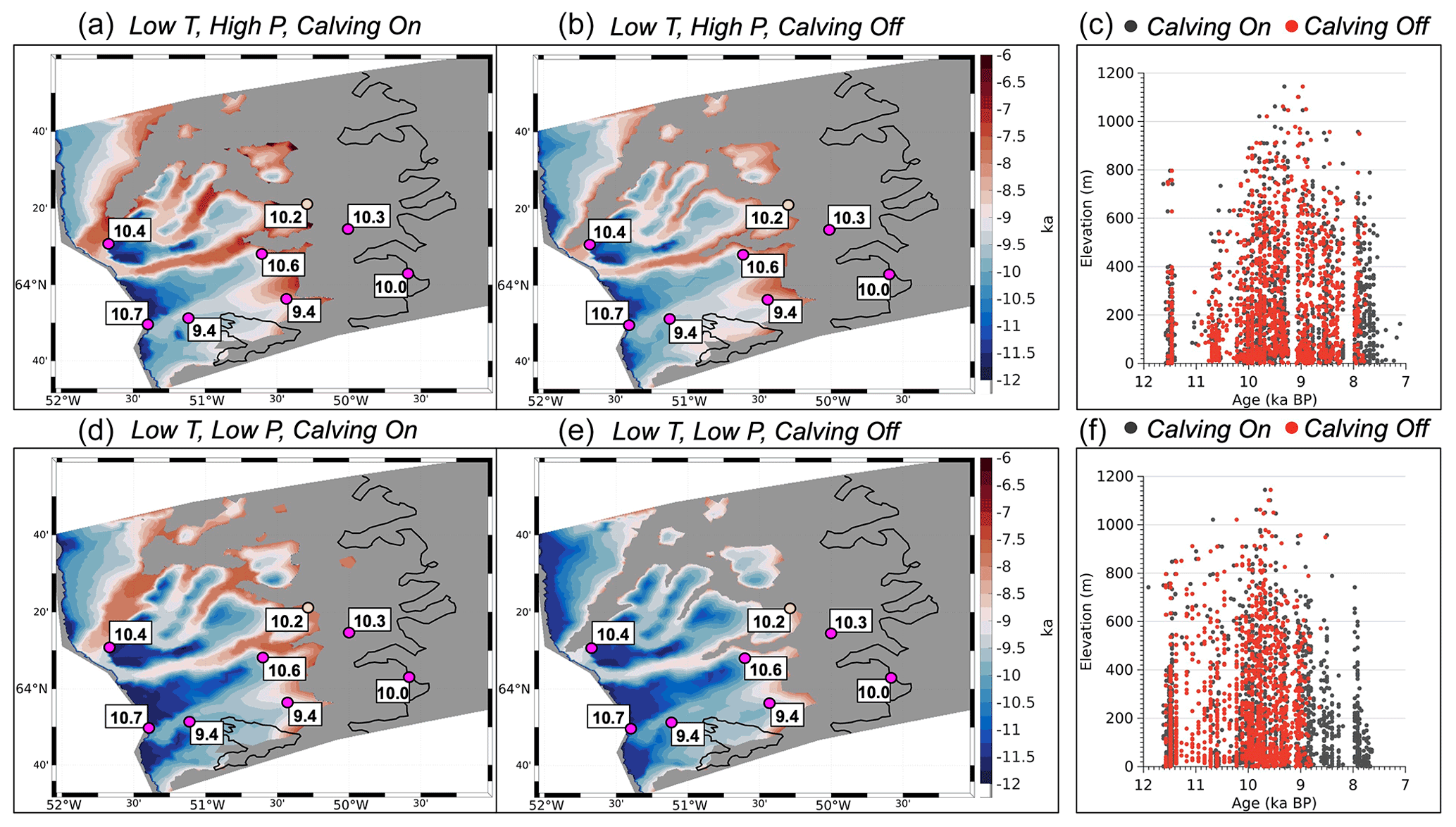
Figure 6 Map of simulated deglaciation ages for low-temperature scenarios with (a) high-precipitation and calving on, (b) high precipitation and calving off, (d) low precipitation and calving on, and (e) low precipitation and calving off. Gray mask is the simulated ice extent at present day, and the black line denotes the actual present-day ice extent (Rignot and Mouginot, 2012). Magenta circles are the best estimate of the timing of deglaciation at that point based on ¹⁰Be surface exposure ages in thousands of years, and the yellow dot shows a minimum limiting radiocarbon age that requires ice-free conditions in the fjord at that time (Weidick et al., 2012; Young et al., 2021). Scatter plot of simulated deglaciation age (above sea level) versus bedrock elevation for (c) low temperature and high precipitation and (f) low temperature and low precipitation. Red dots are from simulations without calving, and black dots are for simulations with calving.

Lastly, it is important to note that simulations that allow calving have a more reduced ice extent (gray mask) at the end of each simulation, which may indicate that calving limits ice-front readvance within the fjord.

The manner in which deglaciation occurs on terrestrial surfaces can be an important factor in determining the pace and magnitude of the ice-margin response to warming. Geologic archives constraining ice retreat across the KNS forefield span an elevational range of 1300 m, yet no elevational dependence on the age of deglaciation is evident (Larsen et al., 2014; Young et al., 2021). To compare our simulated deglaciation history as a function of elevation against the geologic data, we plot the simulated age of deglaciation against elevation and restrict our data points to terrestrial surfaces above sea level (Fig. 5c and f; Fig. 6c and f). In general, our simulations agree with the geologic data, indicating that there was no elevational dependence on the age of deglaciation; if there were any indication of an elevation dependence on the age of deglaciation, we would observe that high-elevation sites would become ice free first, followed by low-elevation sites. Instead, all of the plots show that deglaciation happens simultaneously at discrete time intervals across all elevation bands, indicating that ice surface lowering was rapid and coincident with ice-margin pullback. These elevation–time diagrams also highlight how the higher-precipitation scenarios have later mean deglaciation ages across terrestrial surfaces (Figs. 5c and 6c) than corresponding simulations using the low-precipitation scenario (Figs. 5f and 6f). We also note that for simulations where calving is turned off (red dots), ice retreat appears to stop earlier than for those simulations with calving turned on (black dots). This occurs because the simulations without calving experience a larger Late Holocene ice readvance than those simulations for which calving is turned on (black dots). As a consequence of this, model grid points that would have otherwise deglaciated prior to the readvance are overrun with ice and therefore are not marked as deglaciated in the simulation.

Lastly, each of our experiments end with a simulated present-day ice extent that is beyond (westward of) the actual present-day ice extent (Figs. 5 and 6). Yet the simulated ice-margin position in the fjords is less extensive for all experiments where calving is permitted. Those experiments that allow calving and used the high-temperature scenario (Fig. 5a and d) simulate a present-day ice extent that is closer to the observed present-day margin when compared to simulations using the low-temperature forcing (Fig. 6a and d).

4.2 Ice mass evolution and minimum ice extent

Broadly, scenarios that allow calving undergo greater ice mass loss than those simulations for which calving is not allowed (Fig. 7; black lines). The differences in simulated ice mass also vary depending on the climate scenarios used. For example, during Early Holocene warming (12–8 ka), simulations that allow calving and use the high-temperature scenarios (Fig. 7a and b) experience ice mass loss, while simulations that do not allow calving experience a period of ice mass stability (Fig. 7a and b; dashed red line), which is more prolonged in the simulation using the high-precipitation scenario (Fig. 7a).

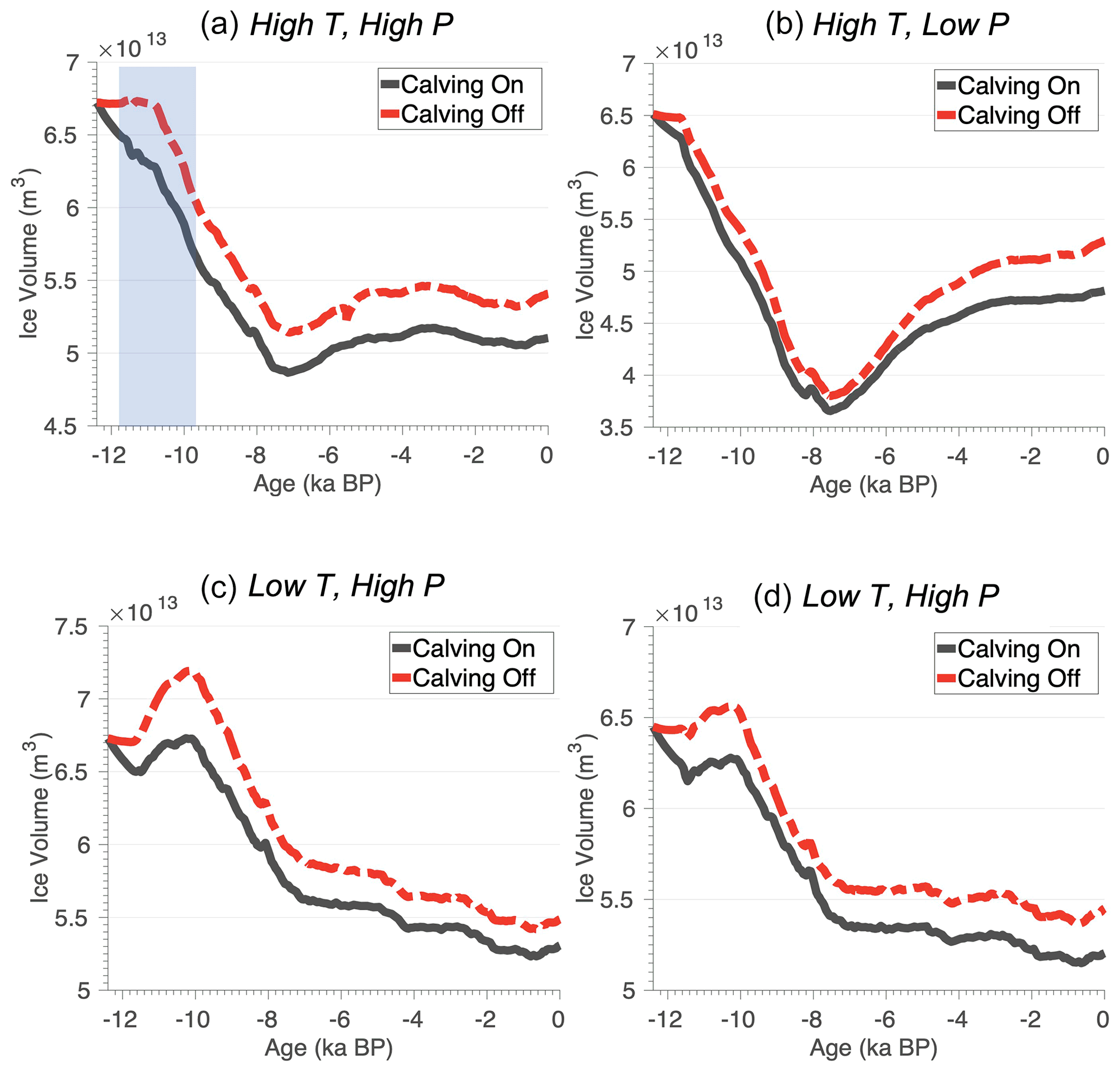
Figure 7 Holocene ice volume (×10¹³ m³) evolution for each model experiment. Refer to Table 1 for a summary of the climate forcings used in each experiment. Black lines denote those simulations with the calving parametrization turned on. Dashed red lines denote those simulations with the calving parametrization turned off. The vertical blue bar above marks a time period (12–10 ka) used for analysis presented in Figs. 8 and 9.

For the simulations using the low-temperature scenario (Fig. 7c and d), initial ice mass loss is interrupted by brief increases in ice mass during the Early Holocene (between 11 and 10 ka). This increase in ice mass occurs for both scenarios with and without calving (Fig. 7c and d; black and dashed red line), although the simulations without calving experience larger increases in ice mass during this period. Accordingly, the low-temperature simulation with higher precipitation (Fig. 7c) experiences larger ice mass gain than the simulation using the low-precipitation scenario (Fig. 7d). During this interval, precipitation is approximately 20 %–30 % more for the high-precipitation scenario during the Early Holocene than the low-precipitation scenario. Much of this mass gain is due to ice thickening over the interior of the model domain, in which despite Early Holocene warming, colder temperatures (at higher elevations on the ice sheet) support snowfall (see Sect. 4.3).

Throughout the remainder of the Holocene, the evolution of ice mass for experiments using the high-temperature scenario (Fig. 7a and b) differ from those simulations using the low-temperature scenario (Fig. 7c and d). Simulations using the high-temperature scenario (Fig. 7a and b) reach a minimum ice volume between 7.6 and 7.2 ka. For the simulation using the high-precipitation scenario, ice mass increases slightly following this minimum and remains generally stable throughout the remainder of the Holocene (Fig. 7a), whereas the simulation using the low-precipitation scenario experiences large ice mass gain following this minimum, with steady growth occurring throughout the remainder of the simulation (Fig. 7b). It is important to note, however, that for the high-temperature scenarios, this ice mass gain is more muted for simulations that allow calving. In contrast, the simulations using the low-temperature scenario (Fig. 7c and d) lose the majority of ice mass by 8–7 ka, with ice mass loss either continuing through the Holocene (Fig. 7c) or remaining relatively stable before reaching a minimum at 0.6–0.4 ka (Fig. 7d).

Regional relative sea-level records reveal that sea level fell below modern levels between 4 and 3 ka before rising towards modern values (Long et al., 2011), interpreted to represent the re-loading of the Earth's crust as the GrIS readvanced during the Late Holocene following a mid-Holocene minimum. In addition, radiocarbon-dated lake sediments from southwestern Greenland suggest that this sector of the GrIS likely achieved its minimum extent after ca. 5 ka and that the eastward retreat of the ice margin was likely minimal (Larsen et al., 2014; Young and Briner, 2015; Lesnek et al., 2020; Young et al., 2021). Although no direct geological constraints on the minimum GrIS ice extent during the Holocene exist, available constraints suggest that the magnitude of large-scale ice-margin retreat inboard of the present-day extent as simulated by some ice sheet models in this sector (20–40 km; Tarasov and Peltier, 2002; Lecavalier et al., 2014) is likely too extreme. Relying on these geologic constraints, we can crudely assess the temporal and spatial patterns of the simulated ice mass and minimum extent.

None of our simulations accurately capture the exact timing of the GrIS minimum in the KNS region, but some simulations are likely better representations than others. Simulations using the high-temperature scenario (Fig. 7a and b) achieve an ice mass minimum prior to 5 ka followed by ice regrowth. The high-temperature and low-precipitation scenario depicts an extreme GrIS minimum followed by significant regrowth. While the overall pattern of a GrIS minimum followed be regrowth is consistent with the geologic record, the magnitude of simulated change is likely inconsistent with geological records, pointing to a rather modest GrIS minimum – although we do acknowledge that minimal ice retreat as constrained by the geologic record does not necessarily equate to muted mass loss. In contrast, the high-temperature and high-precipitation experiment depicts an ice mass minimum that is likely too early, but the magnitude of this minimum is less (Fig. 7a). Moreover, ice regrowth following this minimum is restricted with only modest change occurring over the last 6 kyr (Fig. 7a). Although this simulated minimum is likely too early, a simulated ice mass that undergoes minimal change over the last ∼6 kyr is broadly consistent with the geological record that depicts a minimum closer to ca. 4–3 ka but where the GrIS margin likely did not undergo significant change between ca. 7 and 3 ka (Young et al., 2021). Both low-temperature scenarios are inconsistent with the geological record as both show continued ice mass loss through the Holocene. Although it is possible, but unlikely, that continued ice loss through the Holocene could still be achieved if the ice margin retreated inland followed by a readvance toward its present position, mass loss through the Holocene is inconsistent with relative sea-level records.

The minimum ice-margin extent achieved in our simulations is shown in Fig. 8. For the high-temperature scenarios (Fig. 8a and b), the simulated minimum ice extent is either just outboard of the present-day ice margin (Fig. 8a; high precipitation) or inboard of the present-day ice margin (Fig. 8b; low precipitation). Because the geologic evidence supports the Holocene ice extent minimum being close to and perhaps slightly inboard of the present-day ice margin (Young et al., 2021), both simulations are broadly consistent with the geological record. But, again, the high-temperature and high-precipitation scenario depicts significant ice regrowth resulting in a present-day ice margin significantly more extended than the modern one (Fig. 5).

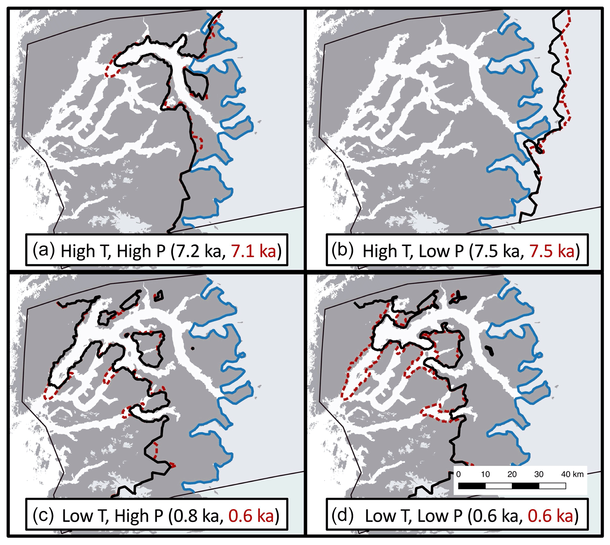
Figure 8 Age of minimum ice extent for each simulation (black text: simulations with calving; red text: simulations without calving). The black line denotes the minimum ice extent for simulations with calving. The dashed red line denotes the minimum ice extent for simulations without calving. The present-day ice extent is shown as the blue line.

4.3 Early Holocene thinning

Figures 9 and 10 show the simulated ice elevation changes for the time period between 12 and 10 ka for each experiment (highlighted in Fig. 7a as the light blue vertical bar). During this time period, widespread Early Holocene warming drove increased ice melt along the margin of the model domain. This pervasive thinning along the margin is captured in all model experiments (Figs. 9 and 10), although the amplitude of ice thinning is greatest for the experiments using the high-temperature scenario (Fig. 9). Across all experiments, inland thickening occurs; however, the magnitude of interior thickening is not solely influenced by the SMB but is also influenced by calving. For our experiments that allow calving, interior thickening is reduced and ultimately influences the trend and magnitude of changes in simulated ice volume; simulations that allow calving either experience increased ice mass loss (Fig. 7a and b) or more muted ice mass gain between 12 and 10 ka (Fig. 7c and d). Additionally, the spatial pattern of elevation changes shows that marginal thinning propagates farther upstream and into the ice sheet interior for simulations that allow ice calving. This relationship continues throughout the remainder of the Holocene as experiments with calving result in either more mass loss than simulations without calving or more muted ice mass gain (see Fig. 7). These variations in simulated Holocene ice mass and ice surface elevation change can be linked to the influence ice calving has on ice-front position and stability, as well as ultimately the rate at which ice can flux through the fjord system. During the time period of 12 to 10 ka, ice velocity differences for simulations with and without calving are in excess of 200 m yr⁻¹ along many fjords within the KNS region (Fig. 11). Calving at the ice front leads to increases in ice velocity within outlets across the model domain, thereby promoting increased mass flux and transport from the ice interior to the margin. Thus, even though the large-scale ice-margin migration across our model domain is relatively insensitive to calving, the overall mass budget and surface profile of the ice is strongly influenced by calving.

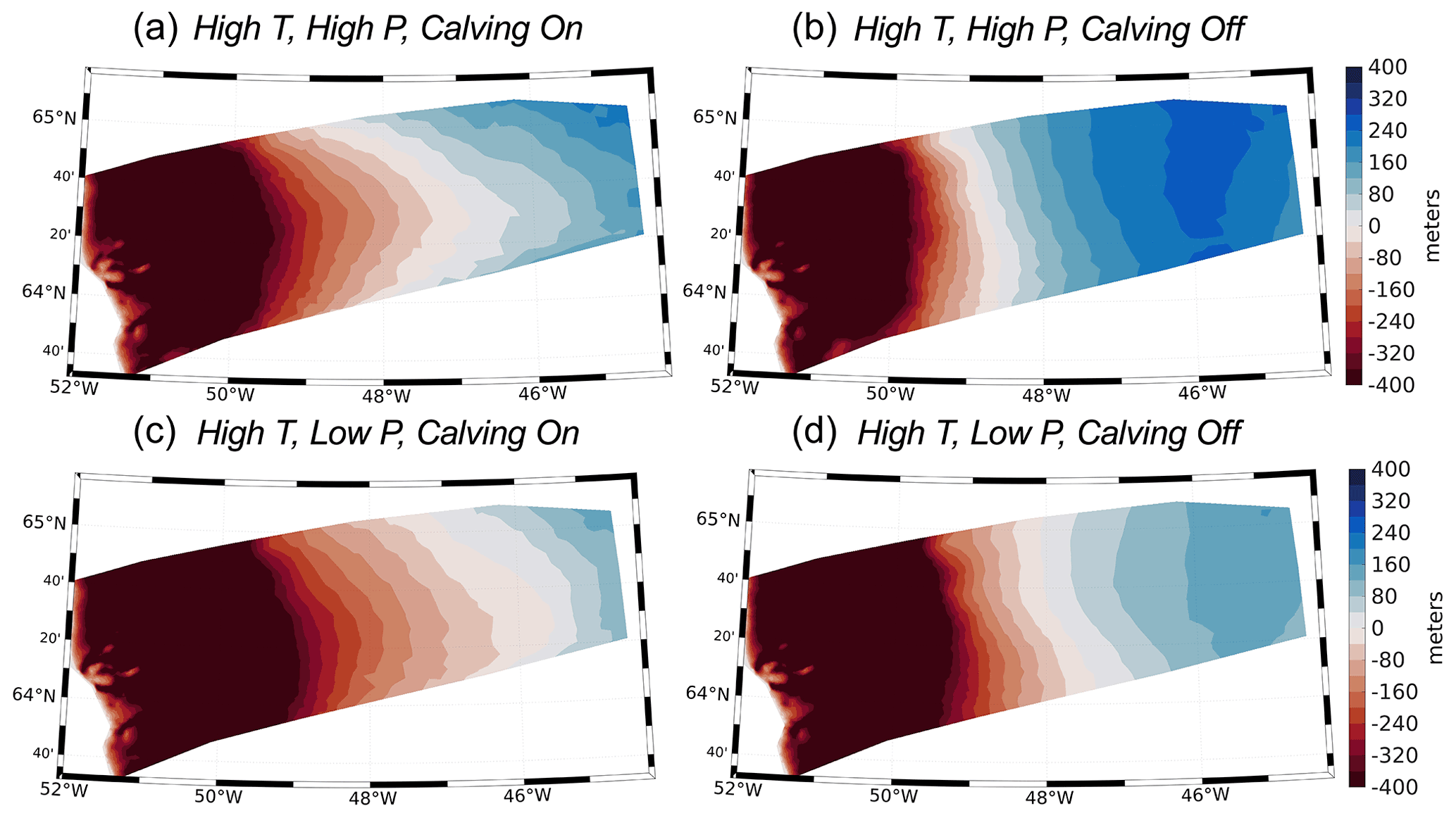
Figure 9 Simulated elevation changes (in m) during the period 12–10 ka shown for experiments using the high-temperature forcing.

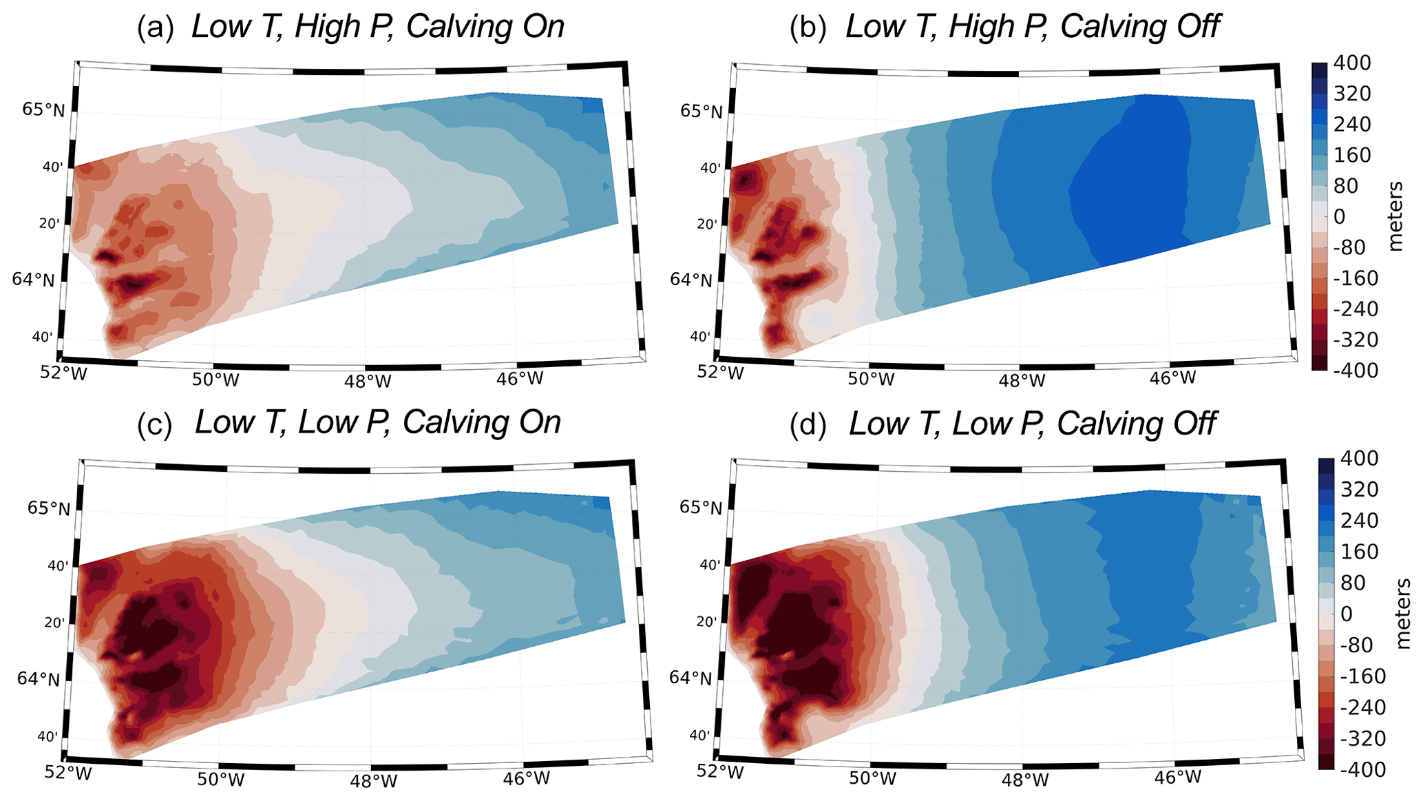
Figure 10 Simulated elevation changes during the period 12–10 ka shown for experiments using the low-temperature forcing.

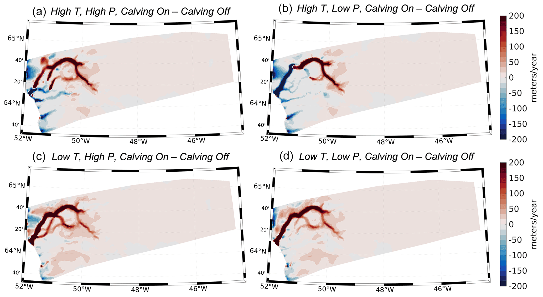
Figure 11 Simulated ice velocity differences between simulations with and without calving for each experiment over the time period 12 to 10 ka. Red colors denote an increase in ice velocity for simulations with calving relative to simulations without calving. Blue colors denote a decrease in ice velocity for simulations with calving relative to simulations without calving.

Reconstructions of Holocene ice thickness across the GrIS are limited, but ice core records provide a long-term perspective of dynamic changes in GrIS elevation at locations at or near the ice divide (Vinther et al., 2009; Lecavalier et al., 2017). For example, some locations experienced more rapid thinning in response to Holocene warming (i.e., Camp Century, Dye 3), while other locations experienced more muted ice elevation changes (i.e., GRIP, Greenland Ice Core Project; NGRIP, North Greenland Ice Core Project). A feature of many of these records, however, is the presence of Early Holocene thickening, potentially triggered by increased snowfall at higher-elevation sites as the climate warmed or by elevation–mass balance feedbacks driven by isostatic uplift (Vinther et al., 2009). Across all model experiments, our simulated timing of inland thickening coincides with thickening experienced at high-elevation ice core locations (Vinther et al., 2009). The magnitude of Early Holocene thickening from ice core records (Vinther et al., 2009; 11.7–10 ka) is on the order of 30–70 m. Therefore, our simulations that allow calving display inland thickening (<120 m) over the time interval 12–10 ka that is more consistent with thickening estimated from ice cores than simulations with no calving (>200 m).

4.4 Sensitivity to marine forcing

Experiments on the tensile strength of ice show that stress thresholds can vary between 150 and 3100 kPa (Petrovic, 2003), with modeling experiments on Jakobshavn Glacier suggesting that the stress threshold for grounded ice can vary between 100 kPa and 4 MPa seasonally (Bondzio et al., 2017). Here, our grounded ice stress threshold is set to 600 kPa. Because our model setup incurs large computational expense, we did not perform a full uncertainty analysis on these parameterizations. Due to the nature of modeled variation in calibrated stress thresholds across Greenland (Choi et al., 2021), however, we ran a small set of experiments in which we set the calving stress threshold on grounded ice to 1 MPa. We performed the transient simulations on the high- and low-temperature scenario cases using the high-precipitation forcing (see Table 1). Additionally, we ran a set of experiments for which the basal melt rate on floating ice was set to 120 m yr⁻¹. Figure 12 shows the simulated ice volumes for these experiments for which the calving stress threshold of grounded ice and basal melt rate on floating ice were changed. These experiments reveal that adjusting the stress threshold from 600 kPa to 1 MPa has no effect on the evolution of the simulated ice volume. Accordingly, increasing the basal melt rate on floating ice has minimal effect on the simulated ice volume (Fig. 12). Ice only begins to float in our experiments when the ice front retreats into the deeper fjord bathymetry within the KNS forefield (see Fig. 3), and therefore submarine melting of floating ice seems to have limited influence on simulated ice mass changes.

Figure 12 Sensitivity to the calving stress threshold for grounded ice and basal melt rates on floating ice. Red line: ice volume evolution for the simulations for which the calving parameterization was turned off. Black line: ice volume evolution for the simulations for which the calving stress threshold for grounded ice is 1 MPa. Gray line: ice volume evolution for the simulations for which the calving stress threshold for grounded ice is 6 kPa. Dashed blue line: ice volume evolution for the simulations for which the basal melt rate on floating ice was set to 120 m yr⁻¹ (with calving stress threshold for grounded ice = 600 kPa).

5 Discussion

5.1 Terrestrial versus marine ice retreat

Southwestern Greenland hosts a rich record of geologic constraints on past ice sheet change (Lesnek et al., 2020). Whereas a series of well-defined moraines constrain Early Holocene ice retreat across portions of southwestern Greenland dominated by terrestrial ice-margin settings (Larsen et al., 2014; Lesnek et al., 2020; Young et al., 2020, 2021), the Kapisigdlit moraine system (Fig. 2: Early Holocene moraines) near the present-day ice margin is the only regionally traceable moraine within the marine-dominated KNS forefield. Instead, ice-margin retreat across the KNS forefield is constrained primarily by minimum limiting radiocarbon ages and ¹⁰Be surface exposure ages on deglaciated bedrock surfaces and glacial erratics (Larsen et al., 2014; Young et al., 2021). The lack of moraine systems between coast and ice is consistent with the relatively high rate of deglaciation estimated from the existing chronology. These chronological constraints detail widespread and rapid retreat of the ice margin across this domain in the Early Holocene, with the ice margin retreating from the coastline around 12 ka to near the present-day ice margin between 10 and 9.5 ka (Young et al., 2021). This relatively rapid retreat based on geological observation is consistent with the lack of an elevation–age relationship in our simulations of ice-margin change.

While the rapid retreat of the terrestrial ice margin is well constrained, how ice retreated up the fjords is less certain. Our simulations depict a pattern of ice retreat across the landscape that was largely independent of ice retreat within fjords, which lagged by 0.5–2 kyr. For our simulations, scenarios using the same climate forcing show little difference (<1 kyr) in the simulated age of ice retreat on terrestrial ice margins regardless of whether calving is allowed (Figs. 5 and 6). The timing and rate of Holocene ice retreat across terrestrial portions of the KNS forefield, however, are strongly dependent on the climate forcing used and ultimately the SMB. The earliest ice retreat occurs in simulations that use the high-temperature scenario. Ice retreat occurs later in simulations that use the low-temperature scenario, which has a delay in the timing and magnitude of Holocene warming (Fig. 4). The pace and magnitude of ice retreat is shown to be modulated depending on precipitation similar to the findings of Briner et al. (2020) and Downs et al. (2020), with delayed and less rapid ice retreat in scenarios with higher precipitation (Figs. 5a and 6a). These results point to the strong influence that climate and, in particular, precipitation can have on modulating the temperature-driven response of Holocene deglaciation. Indeed, select proxy records suggest that southwestern Greenland may have experienced a prolonged period of anomalously high snowfall in the Early Holocene, perhaps driven by increased moisture flux from Baffin Bay and the Labrador Sea as sea-ice extent declined (Thomas et al., 2016). Ice flow modeling across southwestern Greenland has also revealed that elevated precipitation may have accompanied Early Holocene warming (Downs et al., 2020), and recent evidence from a shallow ice core in western Greenland reveals that significant variations in precipitation occurred in the last 2000 years across the margins of the GrIS, whereas this variability is not present in ice core data at the interior of the GrIS (Osman et al., 2021). Because current climate reconstructions employed in paleoclimate ice flow modeling use either simple scaling approaches to reconstruct past climate or rely on information from interior ice cores, large hydroclimate shifts that occur at the ice sheet margin may not be captured (Badgeley et al., 2020). Continued progress in reconstructing past climate will certainly improve our understanding of climatic controls on the long-term response of the GrIS.

In general, simulations using the high-temperature scenario experience terrestrial ice retreat that occurs during 11.5 to 9 ka, a time window consistent with the geological record of ice-margin change in our domain (Larsen et al., 2014; Young et al., 2021). Simulations using the low-temperature scenario reveal terrestrial ice retreat also beginning ca. 11.5 ka, but deglaciation of our model domain continues until ∼7.5 ka. In comparison, geological constraints suggest that by ∼10.3–9 ka the ice margin in the immediate KNS region had already retreated back to, and likely behind, what is the present-day ice margin (Young et al., 2021). Ice surface lowering is captured in all of our simulations, which indicate that on terrestrial surfaces ice retreat was synchronous across low and high elevations. Therefore, the simulated ice retreat could indicate large-scale ice-margin retreat in response to rapid ice surface lowering but certainly precludes scenarios in which ice surface lowering occurred slowly, exposing high-elevation sites well before low-elevation sites. While ice calving does not seem to significantly influence the rate and timing of ice retreat across terrestrial portions of our domain, Late Holocene ice readvance within fjords is more restricted in those simulations that use the calving parametrization. Accordingly, flowband modeling of KNS over the historical period of 1761 to 2012 suggests that marine ice-front retreat was primarily influenced by atmospheric warming and runoff, which helped to trigger ice-front retreat via a crevasse-depth calving criterion, with submarine melting only playing a minor role in historical retreat (Lea et al., 2014a, b). These results do suggest though that climate anomalies were the main driver of historical ice terminus advance and retreat across KNS (Lea et al., 2014b), with our results suggesting that the longer-term Holocene ice terminus position was also primarily driven by atmospheric warming and not through oceanic melting.

5.2 Role of ice calving on mass transport

Mass transport from the ice sheet interior to the margin plays an important role in ice sheet mass change and ultimately its contribution to sea-level rise. Contemporary satellite-derived measurements show inland thickening at high elevations across portions of the GrIS in response to increased snowfall despite pervasive thinning at lower elevations (Smith et al., 2020). Although the response of marine-terminating portions of the GrIS and how it translates to interior ice mass loss can be spatially varying (Williams et al., 2021), thinning at the ice margin due to dynamic or SMB-driven ice loss can elicit changes in driving stresses, which can propagate up glacier and into the interior of the ice sheet (Price et al., 2008; Schlegel et al., 2013; Csatho et al., 2014; Felikson et al., 2020; Williams et al., 2021).

While there is no apparent influence of ice calving on the Holocene ice retreat across the KNS forefield over terrestrial surfaces, our simulations show that ice calving has a significant influence on the evolution of the total ice volume. Ultimately, ice calving leads to an acceleration of ice flow within outlet glaciers that promotes local ice thinning first, followed by propagation of this thinning into the interior of the ice sheet, consistent with contemporary observations (Csatho et al., 2014; Williams et al., 2021). Initially, interior ice surface elevation increases in our simulations, with simulations that allow calving being more consistent with ice-core-derived surface height records (Vinther et al., 2009). Surface lowering near the ice margin driven by a more negative SMB in response to Early Holocene warming causes the ice surface slopes to steepen in our domain, increasing driving stresses and mass transport. This helps drive interior ice thinning, as shown by elevation changes in simulations that allow ice calving (Figs. 9 and 10), leading to increased ice flux at the margin through the ice streams (Fig. 11). This increased mass transport helps limit thinning within outlet glaciers, and where terrestrial locations of our domain become ice free early in the Holocene, ice-front retreat within the fjords lags (Figs. 5 and 6).

Our results suggest that, while calving did not play a significant role in the observed Holocene ice retreat across the KNS forefield, it played an important role in the overall ice mass change across our model domain. These results highlight that the inclusion of physically based ice calving parameterizations is an important step towards modeling the fidelity of simulated ice mass change across paleoclimate timescales. However, the choice of which ice calving parameterization is best suited to Greenland over such timescales is still not well constrained (Goelzer et al., 2017). It remains important though that models maintain high enough spatial resolution in order to capture fjord environments, associated bathymetry, and ultimately ice calving and grounding line migrations over paleoclimate timescales (Cuzzone et al., 2019) as the model resolution can impact simulated ice discharge significantly (Rückamp et al., 2019; Aschwanden et al., 2019).

5.3 Model limitations

Fjord systems in Greenland are typically <5 km in width, making it necessary to implement high-resolution meshes to resolve these features. Our model setup relies on a high-resolution mesh that is able to capture the fjord geometry within the KNS forefield, making it possible to simulate grounding line migration and calving. The calving parameterization used does ignore frontal melting at the grounded ice front. Frontal melt at the base of a calving face has been shown to induce undercutting of the ice front, and it greatly increases calving rates (O'Leary and Christofferson, 2013). For the present day, many of southwestern Greenland's marine-terminating glaciers are not strongly influenced by undercutting (Wood et al., 2021), but this may have been different as ice retreated up the fjord to its present-day location through the Holocene. While proxy records indicate changing sea surface temperatures during the Holocene proximal to our model domain (Axford et al., 2021) and due to a lack of constraints on the long-term subsurface ocean thermal forcing needed to implement undercutting in our simulations, we opted to disregard this. To circumvent this shortcoming, we set our calving stress threshold on grounded ice to a number (600 kPa) that is on the lower end of measured tensile stresses of ice (Petrovic, 2003). Since there was no discernable difference in our simulated ice mass change when a higher calving stress threshold of grounded ice was used (1 MPa), we cautiously assume that implementation of undercutting would have a negligible effect on the calving rates and overall Holocene mass change and ice retreat across our domain. Future work will use a basal melt-rate parametrization (PICOP; Pelle et al., 2019), employed in ISSM currently, to estimate oceanic melt rates from far-field variations in Holocene subsurface temperature and salinity in order to more robustly estimate the impact of oceanic warming Holocene deglaciation across the GrIS.

At the time of this work, ISSM is undergoing improvements and new implementation of solid earth and sea-level feedbacks. While we did not include time-dependent forcings (e.g., Caron et al., 2018) that account for relative sea-level change as we have in prior research (Cuzzone et al., 2019; Briner et al., 2020), future simulations using ISSM will explore the influence of coupled solid Earth–ice feedbacks on ice retreat. Recent ice sheet modeling (Kajanto et al., 2020) showed that the Holocene retreat of Jakobshavn Isbræ was insensitive to relative sea-level (RSL) variations as RSL changes were small in comparison to fjord depth. RSL changes during the Holocene across this domain were relatively small (∼60–100 m at 12.4 ka and decreasing through the Holocene; Caron et al., 2018) compared to fjord depths. Given that ice calving did not seem to largely influence terrestrial ice retreat, we only expect that inclusion of Holocene RSL changes may have influenced ice-front retreat that migrated into deeper waters where floating extensions of the ice front could occur. However, in our sensitivity tests, basal melting on floating ice plays a trivial role in total ice volume changes (Fig. 11) as most of the ice within fjords is grounded during the Holocene retreat.

6 Conclusions

Understanding how climate, calving, and marine processes contribute to ice sheet change across paleoclimate timescales is challenging. Models with lower-resolution meshes are typically favored to ensure computational needs are satisfied. This ultimately leads to poor representation of bedrock topography (Cuzzone et al., 2019; Jones et al., 2020) and grounding line migration (Seroussi and Morlighem, 2018) that control ice flow (i.e., fjords), making the assessment of how ice calving influences large-scale ice-margin change difficult. Moreover, while ice core records provide snapshots of a changing climate at the ice sheet interior, there remain a relative lack of paleoclimate records from the ice sheet margin of sufficient resolution that can be easily incorporated into an ice sheet model's climate forcing.

Here, we presented results from a high-resolution 3D thermomechanical regional ice sheet model that evaluated controls on the behavior of the southwestern GrIS during the Holocene in the vicinity of the KNS forefield, an area with extensive geologic constraints on past ice-margin change. Experiments were driven by novel reconstructions of Holocene climate (Badgeley et al., 2020) and included a physically based ice calving parametrization (Morlighem et al., 2016).

Our modeling results shed light on the well-constrained observations of Holocene ice retreat across the KNS forefield. These simulations agree well with observations that ice retreat on terrestrial bedrock surfaces occurred rapidly between 11.5 and 9.5 ka in response to Early Holocene warming. The variations in the timing and magnitude of ice retreat on terrestrial bedrock surfaces across this region are found to be insensitive to calving within the fjords that intersect this landscape. Instead, the terrestrial ice retreat is more sensitive to the SMB, with warmer climate reconstructions providing the best fit between the modeled and observed ice retreat. Calving, however, does play a significant role in the simulated Holocene ice volume change across this domain. Acting as conduits for mass transport and ice flux, ice velocity within the fjords in the KNS forefield increases when the ice front is allowed to calve. Calving helps promote further ice mass transport from the interior of the domain to the ice front, which helps to thicken ice within the fjords, allowing the ice front to persist longer than adjacent terrestrial margins similar to the ice response simulated for the Holocene retreat of Jakobshavn Isbræ (Kajanto et al., 2020). These results suggest that paleo-ice-flow models that do not sufficiently resolve fjord geometry may not capture dynamic processes that are critical towards understanding long-term ice mass change across the GrIS. Recent ice flow modeling has suggested that despite increased ice mass loss due to a more negative SMB, ice discharge from GrIS marine-terminating glaciers will play a significant role in overall GrIS mass change well into the future (Choi et al., 2021). These results confirm that over paleoclimate timescales, while the SMB may dictate large-scale ice-margin migration as captured in geologic observations, ice discharge has the ability to greatly influence the rate and magnitude of ice mass change. However, as all simulations depict a contemporary ice extent that is too extensive, uncertainties in the reconstruction of past climate and model parametric uncertainties ultimately contribute to misfits that are difficult to quantify given our computationally expensive model setup. Future paleoclimate ice flow modeling with ISSM will aim to take advantage of recent advances in statistical emulation (e.g., Edwards et al., 2021) to better quantify the influence of model parametric uncertainty on simulated Holocene ice retreat.

Geologic archives serve an important role in our understanding of glacier and ice sheet response to climate change. In turn, ice sheet modeling can help improve our understanding of the climatic and ice dynamical factors that led to ice sheet changes preserved by the geologic record. Our modeling results present an exploration of the factors that may have contributed to the observed pattern of Holocene ice retreat across the KNS forefield, echoing that model–data comparisons between ice sheet models and geologic reconstructions can help improve our understanding of long-term ice sheet sensitivity to climatic and dynamic forcing mechanisms.