Impact of runoff temporal distribution on ice dynamics

Record highs of meltwater production at the surface of the Greenland ice sheet have been recorded with a high recurrence over the last decades. Those melt seasons with longer durations, larger intensities, or with both increased length and melt intensity have a direct impact on the surface mass balance of the ice sheet and on its contribution to sea level rise. Moreover, the surface melt also affects the ice dynamics through the meltwater lubrication feedback. It is still not clear how the meltwater lubrication feedback impacts the long-term ice velocities on the Greenland ice sheet. Here we take a modeling approach with simplified ice sheet geometry and climate forcings to investigate in more detail the impacts of the changing characteristics of the melt season on ice dynamics. We model the ice dynamics through the coupling of the Double Continuum (DoCo) subglacial hydrology model with a shallow shelf approximation for the ice dynamics in the Ice-sheet and Sea-level System Model (ISSM). The climate forcing is generated from the ERA5 dataset to allow the length and intensity of the melt season to be varied in a comparable range of values. Our simulations present different behaviors between the lower and higher part of the glacier, but overall, a longer melt season will yield a faster glacier for a given runoff value. However, an increase in the intensity of the melt season, even under increasing runoff, tends to reduce glacier velocities. Those results emphasize the complexity of the meltwater lubrication feedback and urge us to use subglacial drainage models with both inefficient and efficient drainage components to give an accurate assessment of its impact on the overall dynamics of the Greenland ice sheet.

1 Introduction

Since the 2000s a large number of studies have pointed towards large increases in the amount of melt recorded at the surface of the Greenland ice sheet (e.g., Steffen et al., 2004; Mote, 2007; Hanna et al., 2008), which is reflected by the observation of four record-high melts over Greenland in this 22-year period (Nghiem et al., 2005; Mote, 2007; Mernild et al., 2009; Tedesco et al., 2011, 2013a; Tedesco and Fettweis, 2020). Ahlstrøm et al. (2017) identified that a shift in the runoff regime in southwest Greenland took place in 2003 with an 80 % increase in runoff for the following decade compared to the period 1976–2002. The changes in the melt season are clearly observed in the distribution of the melt (Zwally et al., 2011; Sasgen et al., 2012), culminating in the 2012 season when the whole surface of the Greenland ice sheet experienced melt at some point during the year (Nghiem et al., 2012; Tedesco et al., 2013a). But even if it is less visible, the length of the melt season has also been increasing since the late 1970s (Colosio et al., 2021), and that lengthening has a large impact on the overall melt of the ice sheet; this has been clearly pointed out during the exceptionally long 2010 melt season which led to a large amount of total melt (Tedesco et al., 2011).

These changes in the intensity and length of the melt season encourage us to investigate the effect of these changes on the overall mass balance and flow of the ice sheet. To study the impact of surface melt on ice dynamics, we have coupled the Double Continuum (DoCo) subglacial hydrology model to the ice flow model in the Ice-sheet and Sea-level System Model (ISSM; Larour et al., 2012). Studies on alpine glaciers, as well as larger ice sheets, have shown that the meltwater produced at the surface of the ice is routed supraglacially and englacially to reach the base of those glaciers (e.g., Seaberg et al., 1988; Catania et al., 2008; Smith et al., 2015). Once in the subglacial drainage system, these amounts of water have the potential to alter the water pressure at the base of the ice which is a major driver of glacier sliding (e.g. Iken, 1981; Harper et al., 2007; Sole et al., 2011; Vincent and Moreau, 2016). A large water pressure will trigger a high sliding velocity, while a lower pressure will lead to a relatively slower glacier (e.g. Bindschadler, 1983). But the complexity of the subglacial drainage system, and the fact that it can evolve depending on the volume of water that is available, means that increasing the volume of meltwater would not necessarily lead to a constant increase in water pressure and glacier speed (Sole et al., 2013; Tedstone et al., 2015). Increasing water recharge into the subglacial drainage system will lead to an increase in the subglacial pressure until the drainage system reaches a tipping point and reorganizes itself in a more efficient configuration (Walder and Fowler, 1994; Gordon et al., 1998; Mair et al., 2002). At this point, the more efficient drainage system will allow the provided water to drain at a much lower pressure and as such will trigger a deceleration of the overlying glacier (e.g. Anderson et al., 2004; Schoof, 2010).

This threshold behavior leads to the seemingly opposite result of an increase in meltwater availability that can be observed in western Greenland: (i) at high elevations, the larger amount of water routed to the inefficient drainage system at the bed of the glacier will increase the subglacial water pressure and lead to faster glaciers (e.g. Zwally et al., 2002; Doyle et al., 2014), but (ii) at lower elevations, the increased water supply could lead to the prevalence of a more efficient drainage system, leading to lower water pressure in the subglacial environment and a slower ice flow (e.g. Sundal et al., 2011; Sole et al., 2013; Tedstone et al., 2015).

A few observations and modeling studies have confirmed that these different behaviors are linked to the elevation of the measurement and the main subglacial drainage mode (efficient or inefficient) at this location (Bartholomew et al., 2010; van de Wal et al., 2015; de Fleurian et al., 2016). The complexity of the meltwater lubrication feedback hampers its inclusion in Greenland's mass balance projections. The few model simulations that have taken this feedback into account (Shannon et al., 2013; Fürst et al., 2015) implemented a direct link between meltwater availability and ice velocity. Those simulations however do not take into account the spatial discrepancies that are observed, and the use of those simple runoff–velocity relationships are questionable (Truffer et al., 2005). Gagliardini and Werder (2018) used a coupled subglacial hydrology model and ice dynamic model to investigate the response of a glacier in a 40-year simulation. Their simulations focused on the effect of an increase in the intensity of the melt season while keeping its duration constant. It is however unclear if both those factors – melt season length and amplitude – have the same impact on the subglacial drainage system and glacier velocities. The present study focuses on shorter timescales to provide an answer to this question and a better understanding of the meltwater lubrication feedback mechanisms. An improved treatment of this feedback is indeed crucial as the recent study of Gagliardini and Werder (2018) showed that it could account for a volume loss significantly higher than what was estimated from the simple parameterization of Shannon et al. (2013) and Fürst et al. (2015). We can note also that the effect of channelization of the subglacial drainage system has other implications for the evolution of the ice sheet such as the frontal ablation of ocean-terminating glaciers or subglacial erosion for example (Slater et al., 2015; Ugelvig et al., 2018)

We will first give an overview of the components of the model which are specific to this study before describing in more detail the setup and forcing that are used in the study. We then focus on the results from the reference simulation which give us the opportunity to assess the behavior of the system before the impact of the different forcings are presented. Finally we give a broader interpretation of the results of our experiments in light of recent findings on the meltwater lubrication feedback.

2 Methods

2.1 Model

In order to investigate the impact of meltwater availability on ice dynamics we perform coupled subglacial hydrology and ice dynamics simulations within the Ice-sheet and Sea-level System Model (ISSM; Larour et al., 2012). Within the ISSM, the ice flow is treated following the shallow shelf approximation (SSA) (Morland, 1987; MacAyeal, 1989). The choice of this approximation is motivated by a need to run on relatively short time steps, and so it is necessary to have a relatively computationally cheap ice flow model. Since our interest is in the sliding of the glacier (rather than its deformation), SSA is well suited. The lubrication feedback and the impact of subglacial water on ice flow dynamics depends on the choice of the sliding law linking the ice dynamics to the subglacial hydrology. Here we use a nonlinear friction law as described by Schoof (2005) and Gagliardini et al. (2007) which links sliding velocities (u_b) and basal shear stress (τ_b):

$$\begin{array}{}\text{(1)}& {\mathit{\tau }}_b+{\displaystyle \frac{CN|{\mathit{u}}_b{|}^{\left(\mathrm{1}/n-\mathrm{1}\right)}}{{\left(\left|{\mathit{u}}_b\right|+C^n{N}^n{A}_{\mathrm{s}}\right)}^{\left(\mathrm{1}/n\right)}}}{\mathit{u}}_b=\mathrm{0},\end{array}$$

where the parameters A_s and C are the sliding parameter in the absence of cavities and Iken's bound parameter respectively, while n is the rheological exponent in Glen's flow law. Iken's bound (Iken, 1981) represents the maximum value that can be taken by ${\mathit{\tau }}_b/N$ and is only determined by the maximum upslope of the bed. N is the effective pressure which is produced by the subglacial hydrology model in response to the surface melt forcing and corresponds to the difference between the ice overburden pressure P_i and the water pressure at the bed P_w. The subglacial hydrology model used is the DoCo approach as described in de Fleurian et al. (2016). This model is based on a double sediment layer system. In both layers, the water head h_j is computed from a vertically integrated diffusion equation.

$$\begin{array}{}\text{(2)}& S_j{\displaystyle \frac{\partial h_j}{\partial t}}-\mathrm{\nabla }\cdot \left(K_j{e}_j\mathrm{\nabla }{h}_j\right)=Q_j\end{array}$$

The water head depends on the water input (Q_j) and the characteristics of the layer such as its conductivity (K_j), storing coefficient (S_j), and thickness (e_j). In this model, the layer representing the inefficient drainage system (IDS, with subscript j=s) has a low conductivity (K_s) and fixed thickness (e_s). The other layer (with j=e) however represents an efficient drainage system (EDS) with higher conductivity (K_e) which is only activated when the local effective pressure is equal to 0.

Once activated, the thickness (e_e) of this EDS evolves from its initial thickness following equations describing the size of subglacial channels (Röthlisberger, 1972; Nye, 1976) and scaled to take into account the specific geometry of the EDS.

$$\begin{array}{}\text{(3)}& {\displaystyle \frac{\partial e_e}{\partial t}}={\displaystyle \frac{g{\mathit{\rho }}_{\mathrm{w}}{e}_e{K}_e}{{\mathit{\rho }}_{\mathrm{i}}L}}{\left(\mathrm{\nabla }{h}_e\right)}^{\mathrm{2}}-\mathrm{2}A{n}^{-n}{N}^n{e}_e\end{array}$$

The first term of the equation represents the growth of the efficient system by the melting of ice walls through the heat generated by dissipation, where ρ_w and ρ_i are the densities of freshwater and ice, K_e and e_e the conductivity and thickness of the EDS, h_e the water head in the EDS, and finally L the latent heat of fusion of ice. The second term represents the closing of the system through ice creep, where A and n are Glen's parameter and exponent. As the pressure in the EDS decreases, it will get thinner until the point where its transmissivity ($T_e=K_e\times e_e$) is lower than that of the IDS, at which point the EDS is deactivated.

The treatment of the water input Q_j depends on which of the systems is dealt with. The IDS receives water from a specified forcing, whereas the EDS only receives water from a transfer term computed between the two system.

$$\begin{array}{}\text{(4)}& Q_s=Q-Q_t\text{, and }{Q}_e=Q_t\end{array}$$

The water input Q is the sum of the applied surface melt provided by the surface mass balance model described in Sect. 2.3 and a basal melt contribution that is here generated by a constant geothermal heat flux of 0.063 W m⁻². The input to the EDS is due to the transfer of water between layers (Q_t) which depends on the difference of the two-layer water heads such as

$$\begin{array}{}\text{(5)}& Q_t=\mathit{\gamma }(h_s-h_e),\end{array}$$

with γ the leakage time defining the efficiency of the transfer between the two systems.

Finally, the water pressure required to compute the effective pressure is computed from the water head in the IDS as follows:

$$\begin{array}{}\text{(6)}& P_{\mathrm{w}}=h_{\mathrm{w}}\cdot {\mathit{\rho }}_{\mathrm{w}}g,\end{array}$$

where the reference datum for the water head is the mean sea level.

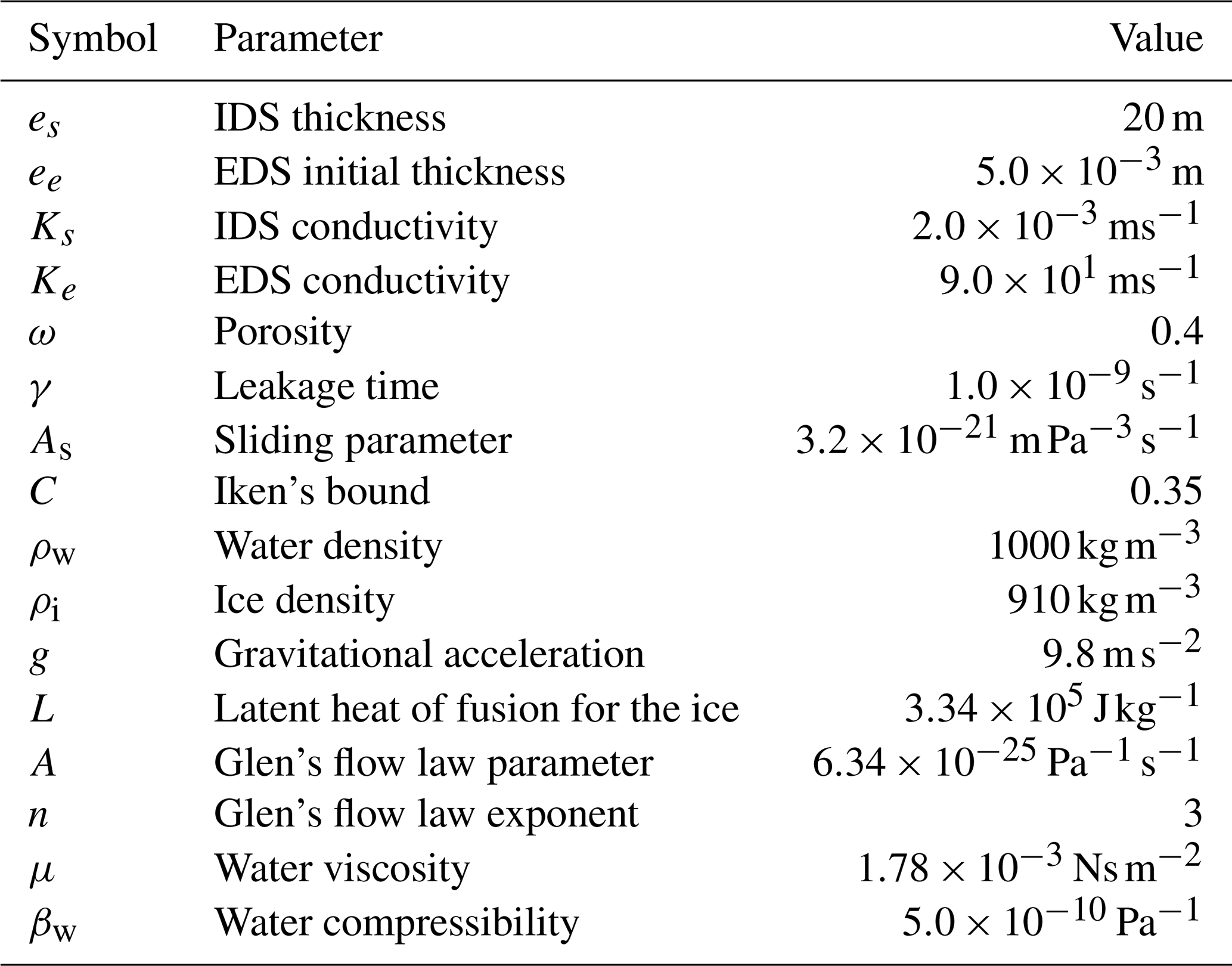
The parameters of the model are given in Table 1, and detailed information about the model can be found in de Fleurian et al. (2016) and de Fleurian et al. (2014).

Table 1 Values of the model parameters.

One challenge when running a coupled ice flow subglacial hydrology model is that the two systems are responding on different timescales. The subglacial hydrology model needs short time steps to achieve stability and provide reliable results, while the ice flow model can run on a longer time step, which saves on computing time. In this study we used a 15 min time step for the hydrology model and a 1 h stepping for the ice flow model. Testing a number of different options showed that this specific combination of time steps gave consistent results while keeping the computational cost at a manageable level. The management of the different time steps for the coupling is performed through the averaging of the effective pressure over the length of the ice flow time step, and the averaged effective pressure is then used to compute the flow. The geometry of the ice model needed as an input to the hydrology model is then kept fixed for the four sub-steps of the subglacial hydrology model.

2.2 Geometry and spin-up

The geometry of the system presented in Fig. 1 is kept as simple as possible in order to obtain a consistent response to applied perturbations. The domain on which the simulations are performed is a synthetic representation of a land-terminating ice sheet margin. The glacier is 150 km long and 20 km wide with a flat bedrock of elevation z_b=465 m and an initial surface elevation z_s defined by a parabolic function.

$$\begin{array}{}\text{(7)}& z_{\mathrm{s}}(x,y)=\mathrm{4.5}\times \sqrt{x+\mathrm{4000}}+\mathrm{186}\end{array}$$

The basal elevation z_b has been chosen to be more representative of the elevation at the front of southwestern Greenland glaciers.

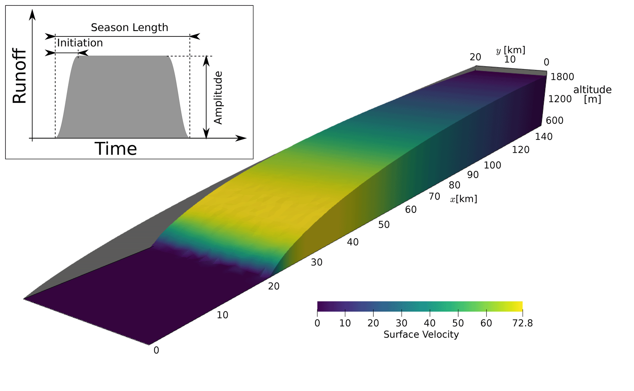
Figure 1 Initial parabolic geometry in grey in the background and final geometry after spin-up. The color represents the mean annual velocities at the end of the spin-up simulation. The inset shows the shape of the temperature forcing used and the different parameters whose impacts are studied.

The parabolic function is chosen such that it resembles the topography of West Greenland as used. From this geometry, a long spin-up is run to achieve stability of the different components of the system. This involved an offline coupling of the ice sheet model in which the surface mass balance was given by the reference forcing described in Sect. 2.3 and the subglacial hydrology model. A relatively stable state with only a small volume loss (0.01 % per year) was attained after roughly 5000 years of simulation. This final state is used for all the perturbation simulations.

2.3 Forcing

Here we take an idealized forcing using the method first described by Hewitt (2013). In this formulation the temperature is first defined at a reference height using the following equation:

$$\begin{array}{}\text{(8)}& \begin{array}{rl}{T}_{\mathrm{ref}}\left(t\right)& ={\displaystyle \frac{r_m}{{\mathrm{\Delta }}_m}}\times \left({\displaystyle \frac{\mathrm{1}}{\mathrm{2}}}\tanh \left({\displaystyle \frac{t-t_{\mathrm{spr}}}{{\mathrm{\Delta }}_t}}\right)\right.\\ & -\left.{\displaystyle \frac{\mathrm{1}}{\mathrm{2}}}\tanh \left({\displaystyle \frac{t-t_{\mathrm{spr}}+{\mathrm{\Delta }}_m}{{\mathrm{\Delta }}_t}}\right)\right),\end{array}\end{array}$$

where

• T_ref is the temperature at the reference elevation of 465 m at the front of the glacier [^∘C],

• Δ_m is the length of the melt season [d],

• r_m is the positive degree day at the reference elevation [^∘C d],

• t_spr is the beginning of the melt season (day 100),

• Δ_t is the length of the initiation of the melt season [d].

The runoff itself is then computed using a given lapse rate:

$$\begin{array}{}\text{(9)}& r(s,t)=max\left\{\mathrm{0},T_{\mathrm{ref}}\left(t\right)\times (z_{\mathrm{s}}-\mathrm{465})\times r_s\right\}\times \mathrm{ddf},\end{array}$$

where r_s is the lapse rate (in ^∘C m⁻¹), and ddf is the degree day factor or conversion rate from temperature to runoff.

The three parameters of this model that we chose to test the sensitivity are the length of the melt season (Δ_m), the positive degree day (PDD) at the reference elevation (r_m), and the length of the initiation (Δ_t) as shown in the inset of Fig. 1. We use the ERA5 reanalysis data to derive a realistic PDD, season length, and lapse rate for our model (Hersbach et al., 2020). First we extracted the daily surface air temperature from 1979 to 2018 for southwestern Greenland at a fixed latitude and for a longitude band going from close to the coast (465 m above sea level) to near the highest point of the land at 2256 m above sea level (67^∘ N, 45–50^∘ W). To calculate the length of melt season for each year we smoothed the daily temperatures using a 15 d midpoint running mean. This smoothing was applied to avoid creating anomalously long melt seasons due to a single day of high temperatures occurring far outside of the rest of the melt season of a given year. The length of the melt season was then calculated using the first and the last day of the year with daily mean temperatures greater than 0 ^∘C. The lapse rate for each day was calculated by taking the gradient of a least-squares linear regression of temperature against elevation across the domain. The daily lapse rate was then averaged for every day when the temperature was above 0 ^∘C at at least one grid point to obtain a typical lapse rate for the melt season. To calculate the PDDs for each year we simply summed the positive temperatures in Celsius over all n levels of the ERA5 reanalysis data within our domain.

$$\begin{array}{}\text{(10)}& \mathrm{PDD}=\sum _{s=\mathrm{1}}^{n}max\left(\mathrm{0},T\left(s\right)\right)\end{array}$$

This procedure gave us a single representative value for the PDD, length of the melt season, and the typical lapse rate for each year from 1979 to 2018. We then fit a normal distribution to the values for all years to determine the mean and standard deviation (SD) of the interannual variability in each of these variables. These were used to define low (mean−SD), medium (mean), and high (mean+SD) values for our sensitivity studies. We also tested the steepness of the temperature variation at the beginning and end of the melt season, which is controlled by the parameter Δ_t and called “initiation” further on in the paper (Fig. 1). Since this cannot be derived from ERA5 data, we instead chose these values pragmatically to create a spread of reasonable seasonal cycles. The different initiation and melt season length are given in Table 2. The value for r_m is presented there with the ratio $r_m/{\mathrm{\Delta }}_m$ which represents the maximum temperature at the reference elevation. With those temperatures, the melt area extends up to 1270 m of altitude for the reference melt intensity and respectively 1209 m and 1355 m for the low- and high-melt-intensity simulations.

Table 2 Values of the different parameters used in the perturbation experiments.

For the simulations with reference PDD, $r_m/{\mathrm{\Delta }}_m$ values for the long and short initiation are respectively 5.96 and 5.74 ^∘C.

Regardless of the length of the melt season we define the summer as the period between days 100 (t_spr, 10 April) and 241, which corresponds to 29 August and is the end of the melt season for the reference forcing.

2.4 Statistics

Due to the nonlinearity of the friction law, combined with the threshold present in the activation of the EDS system, the model results have a significant spread for similar simulations. To extract the characteristic evolution of the system we perform an ensemble of simulations for each parameter set. Each ensemble contains 100 simulations which only differ in their starting time, which is shifted 1 min for each simulation. This sampling allows us to get similar simulations while still keeping the natural variability of the model. The different starting time leads to every simulation having results on slightly different time steps. To remedy this problem, and to ensure that the results are not shifted in time, all the simulations are synchronized on the same time steps through linear interpolation before any further analysis. The distribution of the simulations that are produced through this procedure do not yield a normal distribution as seen in Fig. 2. To overcome this distribution issue, we decided to use the Wilcoxon signed-rank test to investigate the difference of every parameter set to the reference simulation. We use a non-parametric Wilcoxon signed-rank test to assess the differences between the reference simulation and the perturbed simulation and test if the perturbations lead to significant differences in the response of the model. Every time that the differences from one simulation with respect to the reference are said to be significant (Table 3 to 6), it means that the null hypothesis of the Wilcoxon signed-rank test (the median of the differences is zero) is rejected with a 99 % confidence level.

3 Results

3.1 Reference simulation

The reference simulation uses the medium value for the length and intensity of the melt season, as well as a 10 d period for the initiation of the melt season as reported in Table 2. Figure 2 shows the evolution of the mean runoff, ice velocity, and effective pressure, together with the point of highest active EDS throughout the simulations. The highest active-EDS point corresponds to the surface elevation of the farthest inland location where the EDS is active at any time in the simulation. This variable is a good indicator of both the spread of the EDS but also of the dynamics of its development and collapse throughout the seasons.

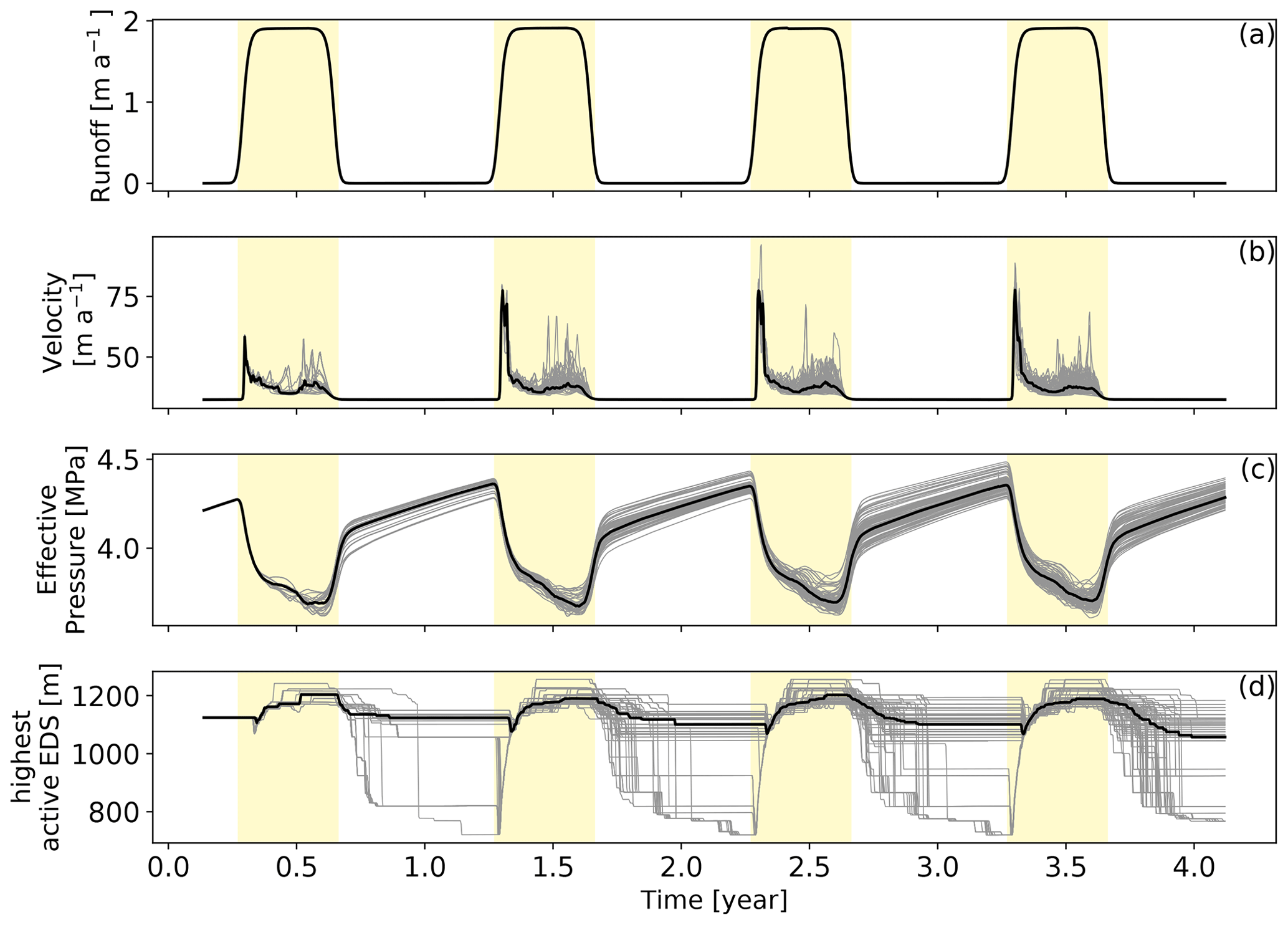
Figure 2 Evolution of the surface runoff (a), ice velocity (b), effective pressure (c), and highest active efficient drainage system node (d). All panels show spatial means over the whole domain. The yellow shading represents the summer period, while every grey line corresponds to one member of the ensemble of simulations, and the thick black line represents the median of the ensemble.

In this figure we show each individual simulation as a grey line, and the mean value of the ensemble is represented by the thick black line. The general evolution of the mean velocities on the whole domain is similar for every year of the simulation as shown in Fig. 2b. The first year of the simulation shows a slightly lower spring speedup event which is related to the relaxation of the geometry from the spin-up. In the following we will focus on the second year of the simulation, which is the one that was perturbed for the sensitivity experiments. As the melt season starts (yellow shaded regions of Fig. 2), runoff increases, building up basal water pressure under the ice and triggering a drop in effective pressure leading to a sharp speedup of the glacier. The decrease in the effective pressure (Fig. 2c) slows down as the efficient drainage system develops, and it drains higher regions of the glacier (Fig. 2d). The velocities then quickly subside as the efficient drainage system develops in the lower part of the glacier and extends upstream. After this first speedup event, the velocities tend to stabilize to a lower level, with each simulation showing some later velocity spikes which tend to occur more often at the end of the melt season. These higher velocities are due to the continuous lowering of the effective pressure throughout the melt season. These spikes are linked to a secondary reduction in the effective pressure which happens when the EDS is fully developed, and so the water going into the system tends to overload this system. These accelerations have been observed in Greenland where it is usually linked to more important melt or rainfall events after the development of an efficient drainage system (e.g. Cowton et al., 2013; Doyle et al., 2015; van de Wal et al., 2015). We will further refer to this late acceleration phase as the autumn acceleration. At the end of the melt season, the drop in runoff leads to a fast increase in the effective pressure which goes back to its winter level.

The evolution of the mean variables over the whole glacier are however not representative of their local evolution. In Fig. 3 we show the evolution of the velocity and effective pressure at four different altitudes in the domain. These figures show two main behaviors for those two variables. The lowest part of the glacier, closer to the front (at 465 m of altitude), is characterized by a strong spring speedup (Fig. 3b–c), whereas the higher region of the domain shows a more gradual increase in velocities throughout the melt season (Fig. 3d–e). These different responses in velocity are driven by the effective pressure at the base of the glacier. At the lower elevations (Fig. 3g–h), the effective pressure shows a sudden drop at the beginning of the melt season followed by a quick rebound when the efficient drainage system activates, which drives the spring speedup event. At higher elevations (Fig. 3i) the decrease in effective pressure is more gradual, and it does not reach values low enough to trigger a spring speedup event or lead to the activation of the efficient drainage system. Even higher up on the glacier the effective pressure is driven by downstream activity as there is no runoff at these elevations. As a result, the effective pressure shows very small variations which get more and more out of phase with the melt season as we go higher up the glacier (Fig. 3j). At the lower elevations (Fig. 3g–h) and at the end of the melt season, we see an overshoot of the effective pressure winter values as the subglacial drainage capacity is higher than the recharge at this time. We will in the following use the acceleration of the glacier as a reference metric to define the elevation at which the glacier shifts from the spring speedup-driven velocity pattern to the more gradual one. This shift in behavior corresponds to the maximum elevation at which a spring speedup is observed (SSU_max). The threshold to define SSU_max is set from the reference simulation ensemble as the altitude at which the glacier acceleration at the beginning of the melt season drops under 20 $\mathrm{m}{\mathrm{a}}^{-\mathrm{1}}{\mathrm{d}}^{-\mathrm{1}}$ which is shown by the white line in all panels of Fig. 4. In the reference simulation, SSU_max is encountered at 1058 m, and throughout the different simulations its elevation varies between 1000 and 1150 m.

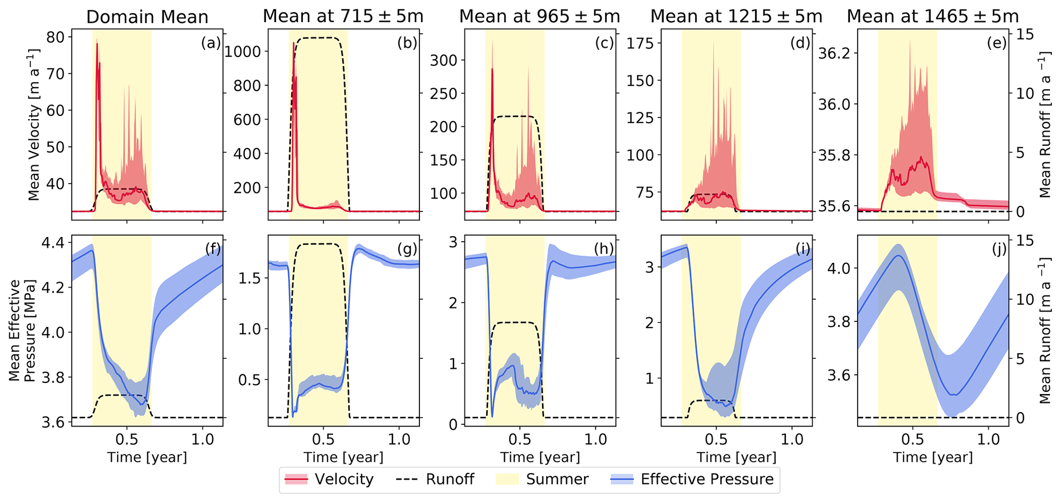
Figure 3 Evolution of the velocity (a–e) and effective pressure (f–j) for the second year of the simulation. The different columns present values at different altitudes, and the mean value in the domain is given for reference. The dashed black line shows the runoff at each elevation on the right axis; the range of the left axis (for velocity and effective pressure) varies in the different panels. The yellow shading represents the summer as defined in Sect. 2.3

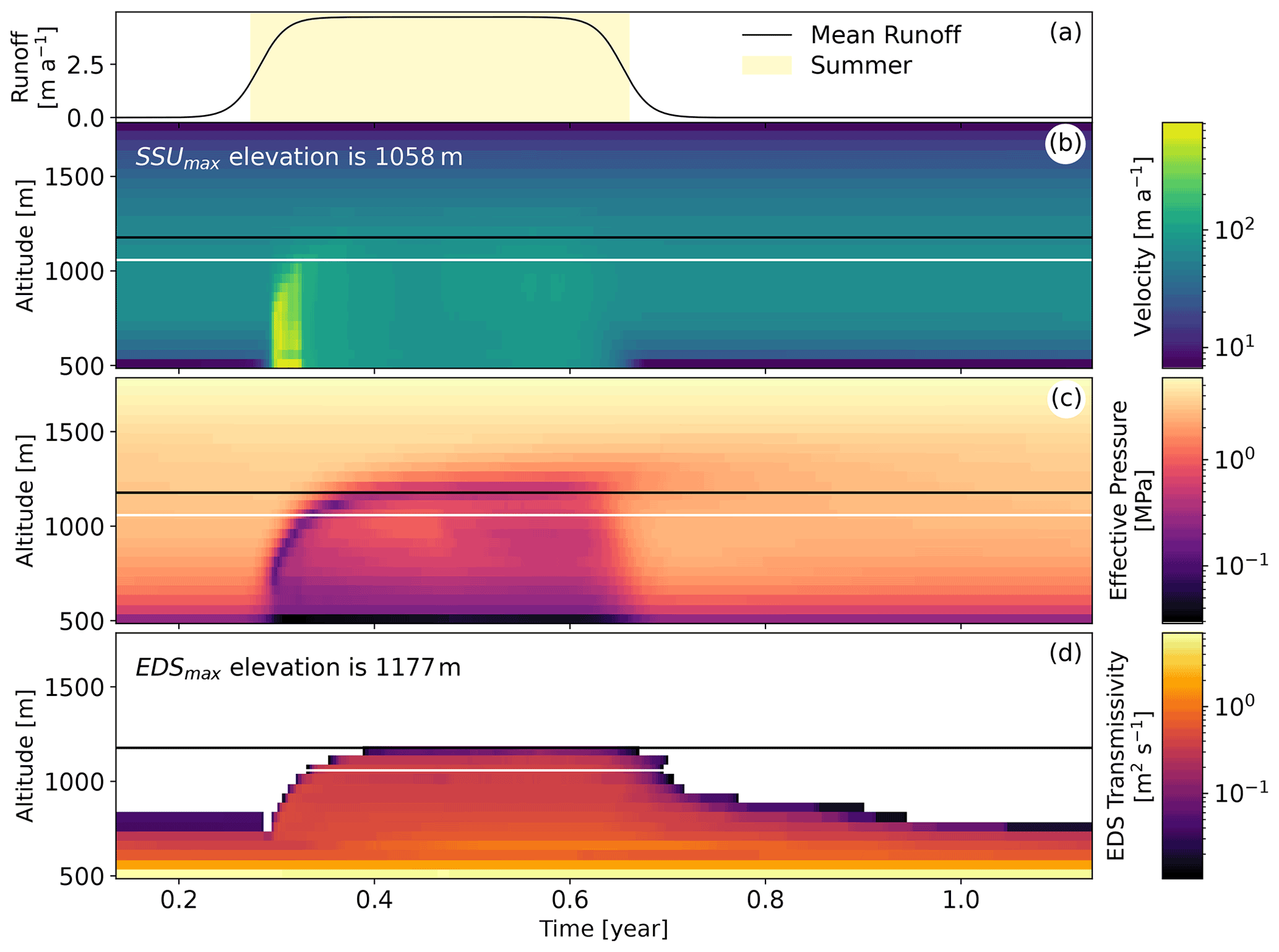
Figure 4 Evolution of the velocity (b), effective pressure (c), and efficient drainage system transmissivity (d) binned in 50 m elevation bands. The runoff is given in panel (a) for reference. The white line across panels (b) to (d) represents SSU_max as defined in Sect. 3.1. The black line across panels (b) to (d) represents the maximum altitude at which the EDS is activated (EDS_max).

We can also observe the two different behaviors of the system in Fig. 4. Here we see that the fast spring speedup is confined below the SSU_max elevation (white line in all panels), as expected from its definition (Fig. 4b). The EDS transmissivity (Fig. 4d) is a proxy for the capacity of the subglacial drainage system to drain water. The white region corresponds to periods when the EDS is not active, while the higher values indicate a highly developed and efficient system. The lowering of the transmissivity at the end of the melt season shows how a drop in water pressure leads to the contraction of the EDS and ultimately to its collapse and deactivation. From the EDS transmissivity we can define the maximum altitude at which the EDS is activated (EDS_max). EDS_max is slightly higher than SSU_max and is the effective boundary between the lower part of the glacier, where the effective pressure is mostly controlled by the efficient drainage system, and the upper part of the glacier, where the effective pressure evolution shows a more gradual evolution in line with the weaker conductivity of the inefficient drainage system.

3.2 Melt season length forcing

We first investigate the effect that a shorter or longer melt season has on the glacier's velocities. For this set of simulations, we wish to investigate the effect of changes in the melt season length, independent of changes in the integrated melt volume, so we vary the melt intensity inversely with the melt season length. This choice allows us to compare both the length and intensity of the melt season and investigate which parameter has the stronger effect on the glacier's velocity. In Sect. 3.3 we will present more details about the specific impact of a change in melt intensity or melt season length when they are applied separately. Figure 5 presents the comparison between the reference simulation (grey), the long and low-intensity melt season (red), and the short and high-intensity melt season (blue), which are shown for two different altitudes.

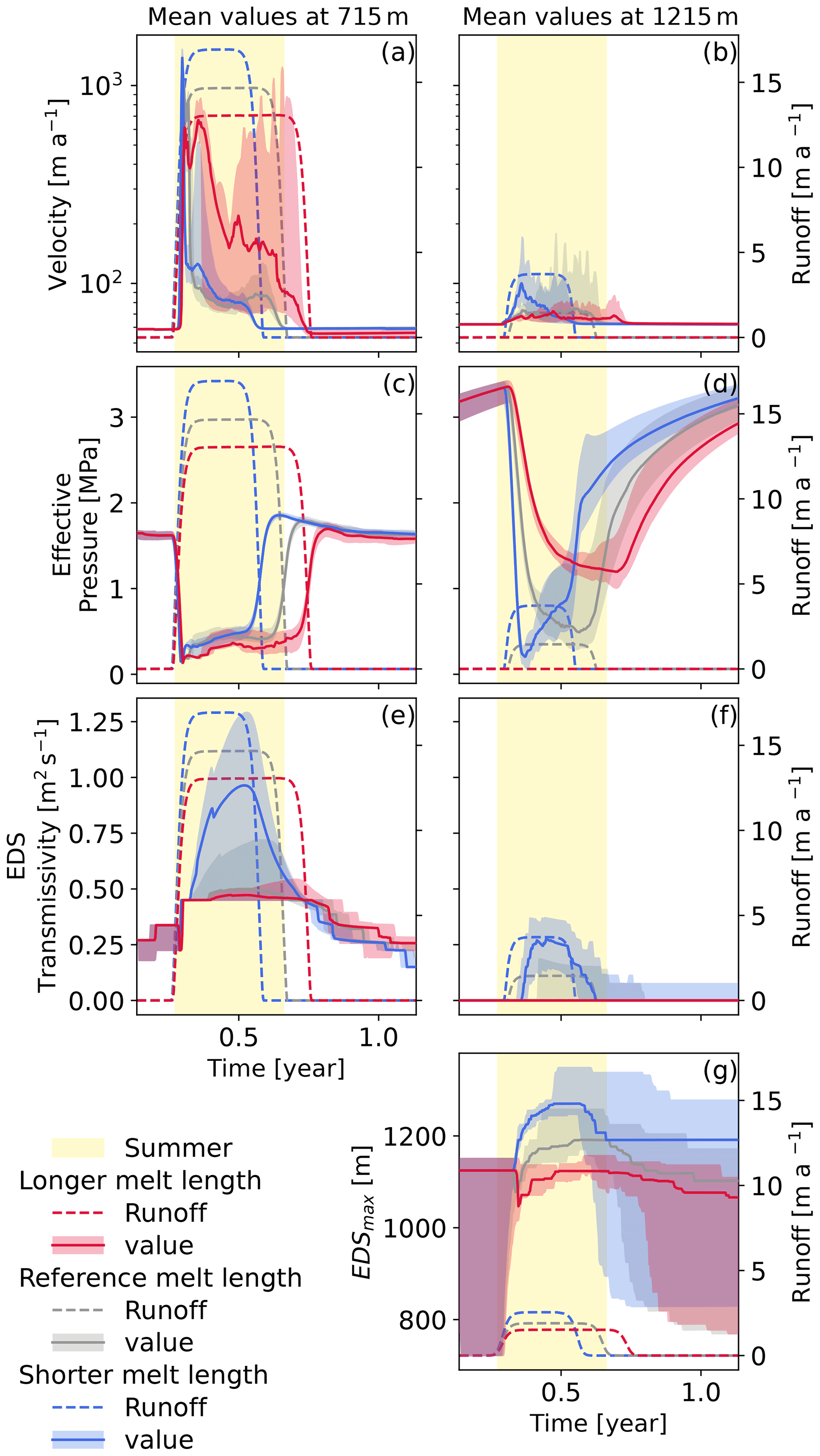
Figure 5 Evolution of the velocity (a–b), effective pressure (c–d), and efficient drainage system transmissivity (e–f) at two different altitudes. Evolution of the maximum height of the active EDS (g). Every panel shows the reference simulation in grey, the longer, lower-intensity melt season in red, and the shorter, higher-intensity melt season in blue. The same color scheme is used for the runoffs which are shown as dashed lines and are referenced on the right axis. The yellow shading corresponds to the fixed summer duration as defined in Sect. 2.3.

Starting with the velocities we see quite a different evolution for the long and short melt seasons with a distinct evolution above and below the SSU_max elevation. We must note here that SSU_max also varies with the different forcing, ranging from 996 m for the longest melt season to 1100 m for the shortest one as reported in Table 3. At low elevation, the shorter and more intense melt season leads to a sharper, shorter-lived, but also more intense spring speedup (Fig. 5a). This differs with the evolution modeled for the longer melt season in which the spring speedup is less marked initially and followed by a second acceleration event. Contrasting with that, the end of the melt season and the beginning of winter show an acceleration for some of the simulations forced by the long melt season as seen by the red shading in Fig. 5a, whereas the early shutdown of the short melt season leads to slow velocities at the end of summer with no simulations showing re-acceleration at this time. At 1215 m, which is above SSU_max for all simulations, the velocity evolution is quite different. While the reference simulation only showed a small increase in velocities, there is quite a large acceleration for the intense melt season, with some simulations showing high velocities throughout the melt period. This contrasts with the reference simulation in which there was no speedup at the initiation of the melt season but a more gradual build-up of velocities until the glacier reached its maximum velocities at the end of the melt season. At the other end of the spectrum, the long but less intense melt season leads to lower velocities than the reference at the beginning of the melt season, but this low acceleration is sustained throughout the melt period. The differences that are observed in the velocity evolution for the different altitudes and melt season lengths are explained by the evolution of the effective pressure which is tightly linked to the efficiency of the draining system. Below SSU_max, the effective pressure shows a drop early in the melt season for both perturbed scenarios. However, the effective pressure recovers faster for the shorter (and more intense) melt season in which it quickly rebounds to a summer value plateau. This contrasts with the long melt season in which the summer plateau is reached later and not after a second reduction in effective pressure due to the second acceleration event. The EDS transmissivity is responsible for these dynamics, whereby the higher intensity of the shorter melt season allows the glacier to quickly develop a very efficient subglacial draining system which enables a fast rebound of the effective pressure. The greater efficiency of the EDS for the short melt season is also apparent in the EDS_max evolution (Fig. 5g) in which the shorter melt season leads to a faster development of the EDS towards higher elevations than the one reached in simulations with longer melt seasons. We note also that with a more developed efficient drainage system (Fig. 5e) the overshoot which is observed at the end of the melt season (Fig. 5c) is more marked, with the highest overshoot observed for the more intense melt season. This overshoot leads to the lowest velocities being reached just at the end of the melt season, and the ice flow then accelerates throughout the winter.

At higher elevations, the changes in the length and intensity of the melt season lead to a contrasting evolution for the effective pressure. For the short melt season, the response is similar to the one that was observed at lower elevation. Indeed, at this elevation the runoff is quite substantial, leading to the rapid decrease in the effective pressure at the beginning of the melt season. The effective pressure then reaches values that are low enough to activate the EDS as seen in Fig. 5f and g, which in turn drives the strong increase in effective pressure. In terms of velocities, the variations in effective pressure drive a fast flow at the beginning of the melt season which quickly subsides. The reference and the longer melt season show quite a different behavior regarding their effective pressure. For those simulations, the runoff at this altitude is too low to trigger the activation of the EDS. This leads to a gradual decrease in the effective pressure throughout the melt season which only increases again when the melt season ends. This pressure evolution induces moderate summer velocities that last throughout the melt season.

Table 3 Velocity difference from the reference simulation for different melt season lengths and intensities. The values in bold fonts are the simulations for which the difference with respect to the reference simulation is significant as per a Wilcoxon test with p=0.01. The summer and winter are defined as fixed periods, with summer starting on day 100 and ending on day 241, while winter covers the rest of the year.

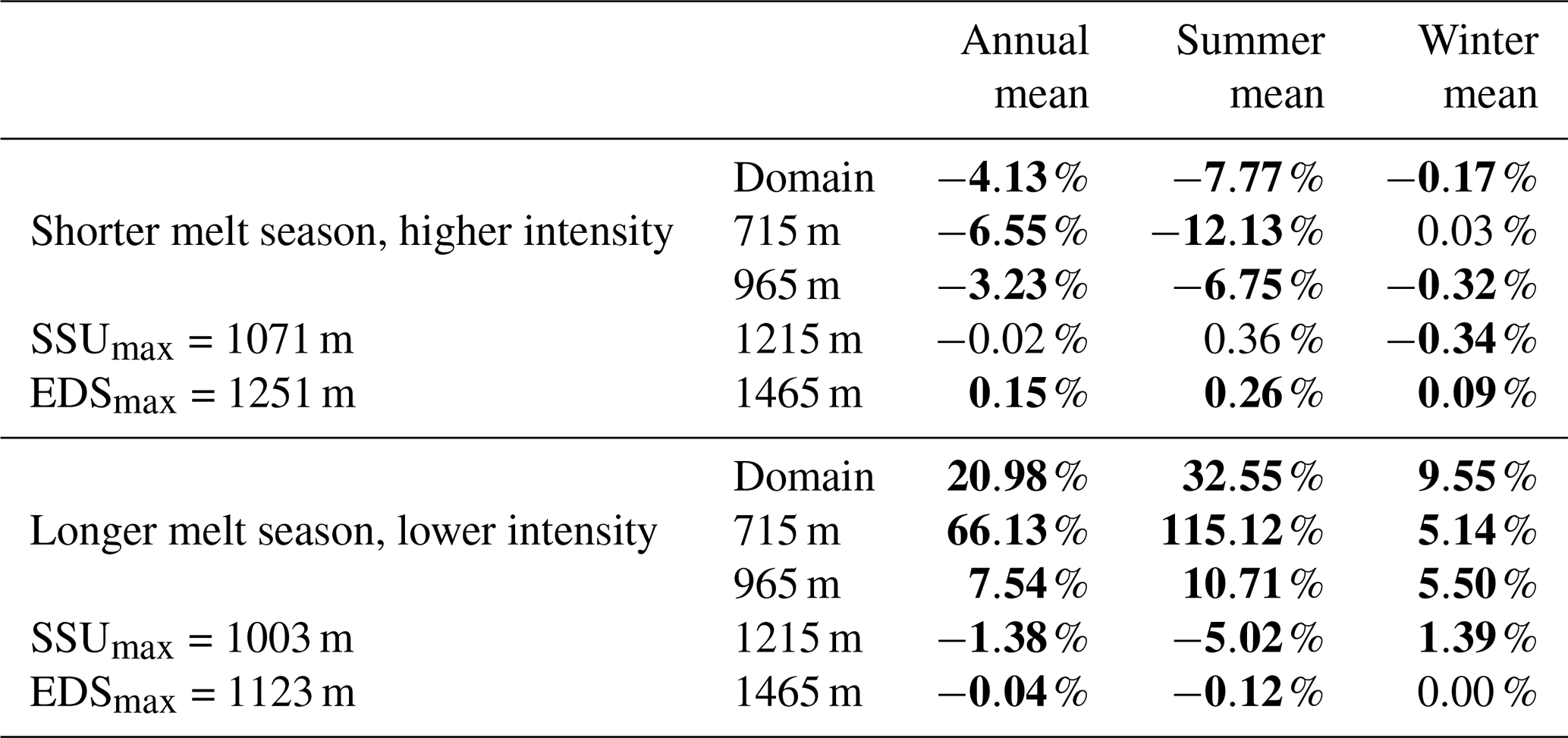
Table 3 summarizes the impact of the length of the melt season on the dynamics of the glacier. The shorter and more intense melt season shows a significant reduction in the overall glacier velocity which is mostly driven by a reduction in the summer velocities below the SSU_max altitude (1071 m in this case). In the case of the long melt season, the acceleration of the glacier is mostly driven by the summer acceleration of the lowest parts of the glacier. There is a slight deceleration at higher elevations, but that is not sufficient to offset the doubling of the mean summer velocities that is observed during summer at the lowest elevations. The winter mean velocities of the longer melt season experiments are somewhat deceiving as the longer melt season means that part of the melt is now happening during the so-called winter. Coming back to Fig. 5a it is clear that the winter velocities in this case are significantly lower than in the other simulations, which is in line with the behavior shown by Sole et al. (2013) in southwest Greenland. It is interesting to note here the reversed pattern in the velocity variations with the altitude, in which the shorter and more intense melt season leads to a slower glacier at low elevations and faster at higher elevations and in which the reversed response is observed for a longer, less intense melt season. In both cases however it is the summer velocities at low elevations which are driving the changes in the annual velocities of the glacier.

3.3 Intensity vs. length

In order to discriminate between the intensity and length of the melt season we release the requirement that the runoff must be equal in all simulations. First we run a series of experiments with the same intensity but in which the length of the melt season varies (Fig. 6). Second, we keep the melt season length fixed but vary the intensity (Fig. 7).

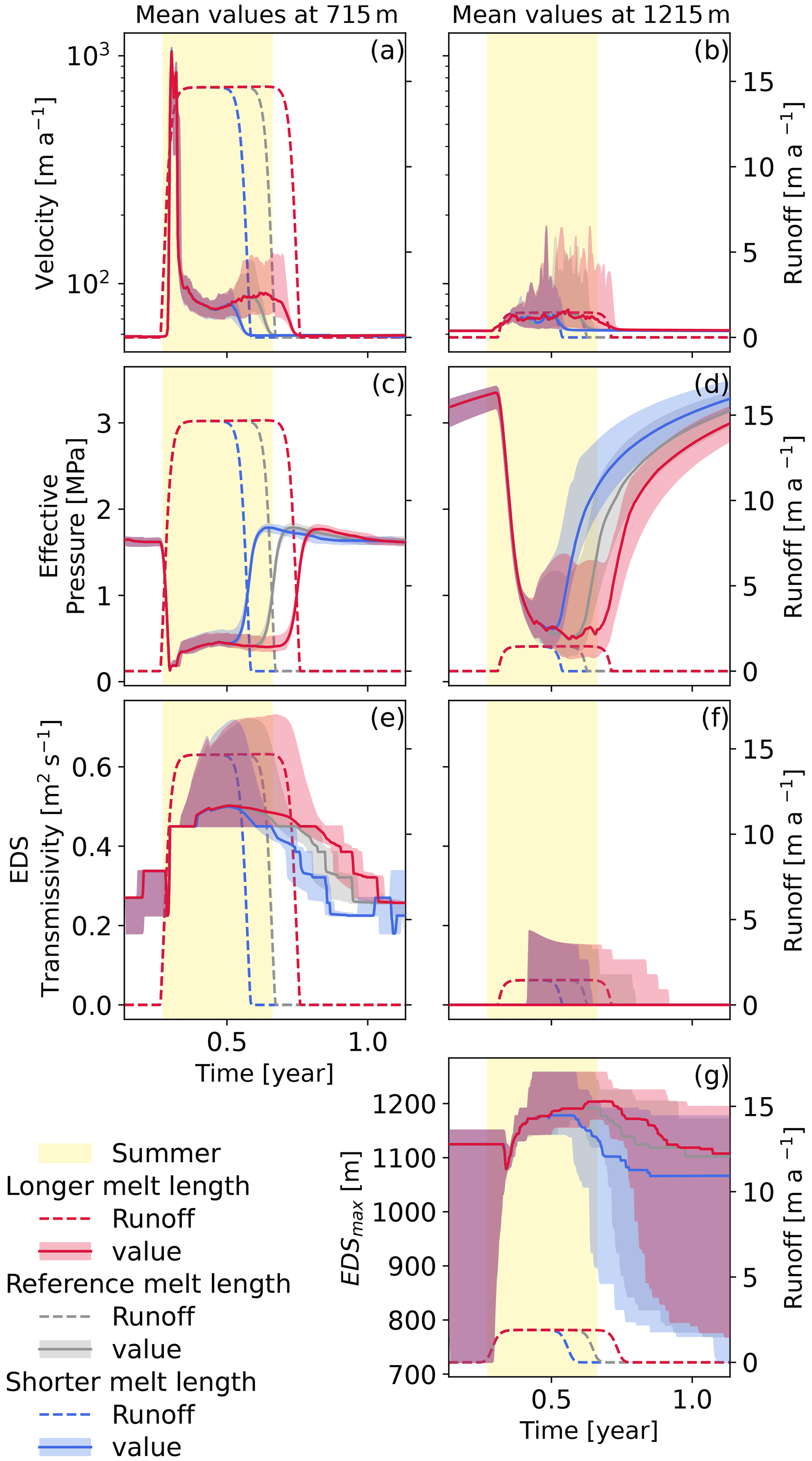
Figure 6 Evolution of the velocity (a–b), effective pressure (c–d), and efficient drainage system transmissivity (e–f) at two different altitudes. Evolution of the maximum height of the active EDS (g). Every panel shows the reference simulation in grey, the longer melt season in red, and the shorter melt season in blue. The same color scheme is used for the runoffs which are shown as dashed lines and are referenced on the right axis. The yellow shading corresponds to the fixed summer duration as defined in Sect. 2.3.

As expected the evolution at the beginning of the melt season of those experiments is very similar as they are all experiencing the same forcing. The simulations start to differ at the point when the short melt season ends. At this time, the effective pressure for this simulation goes back to its winter level with a slight overshoot (Fig. 6c). This timing also coincides with a period during which the effective pressure of the two longer melt seasons is dropping again. This decrease seems to be due to the efficiency of the drainage system reaching a maximum before slowly decreasing and driving the effective pressure down (Fig. 6e). The effect of this effective pressure decline is transferred to the ice velocities for which we see an accelerating trend at the end of summer for the simulations with the longer melt seasons (Fig. 6a). At higher elevations the overall behavior of the glacier is not strongly impacted by the change in melt season length. At lower elevations, when the simulation with the shortest melt season finishes the melt season, the effective pressure goes back to its winter levels, while the simulations with longer melt seasons have a continued decrease in the effective pressure (Fig. 6d). In terms of velocity, only the duration of the summer acceleration is significantly different under different forcings, with a mean summer velocity that is comparable for all simulations (Fig. 6b). However, while the median summer velocity is similar for all simulations, individual ensemble members with large acceleration events late in the melt season are more common in the longer melt season.

Table 4 Velocity difference from the reference simulation for different melt season lengths and reference intensities. The values in bold fonts are the simulations for which the difference with respect to the reference simulation is significant as per a Wilcoxon test with p=0.01. The summer and winter are defined as fixed periods, with summer starting on day 100 and ending on day 241, while winter covers the rest of the year.

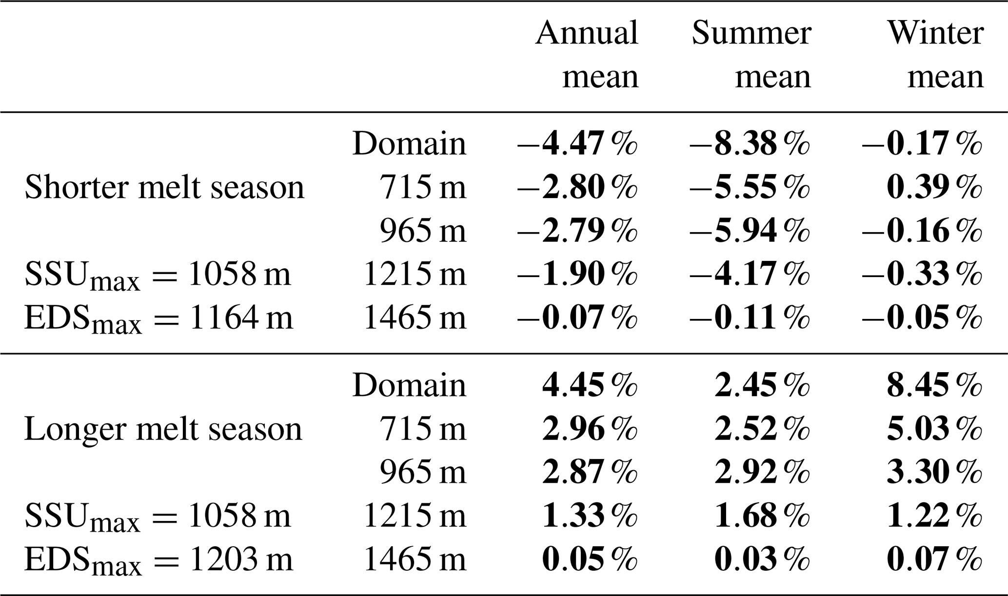
The overall changes in velocities are presented in Table 4, contrasting with the experiments performed with a constant PDD, and we see here that the changes in the melt season length act in the same direction (either acceleration or slowdown) at all altitudes. We also note that the symmetry in the forcing difference leads to a linear response in term of velocities in which the annual mean velocities for the shorter melt season forcing are decreased by a similar amount with respect to the reference simulation and vice versa.

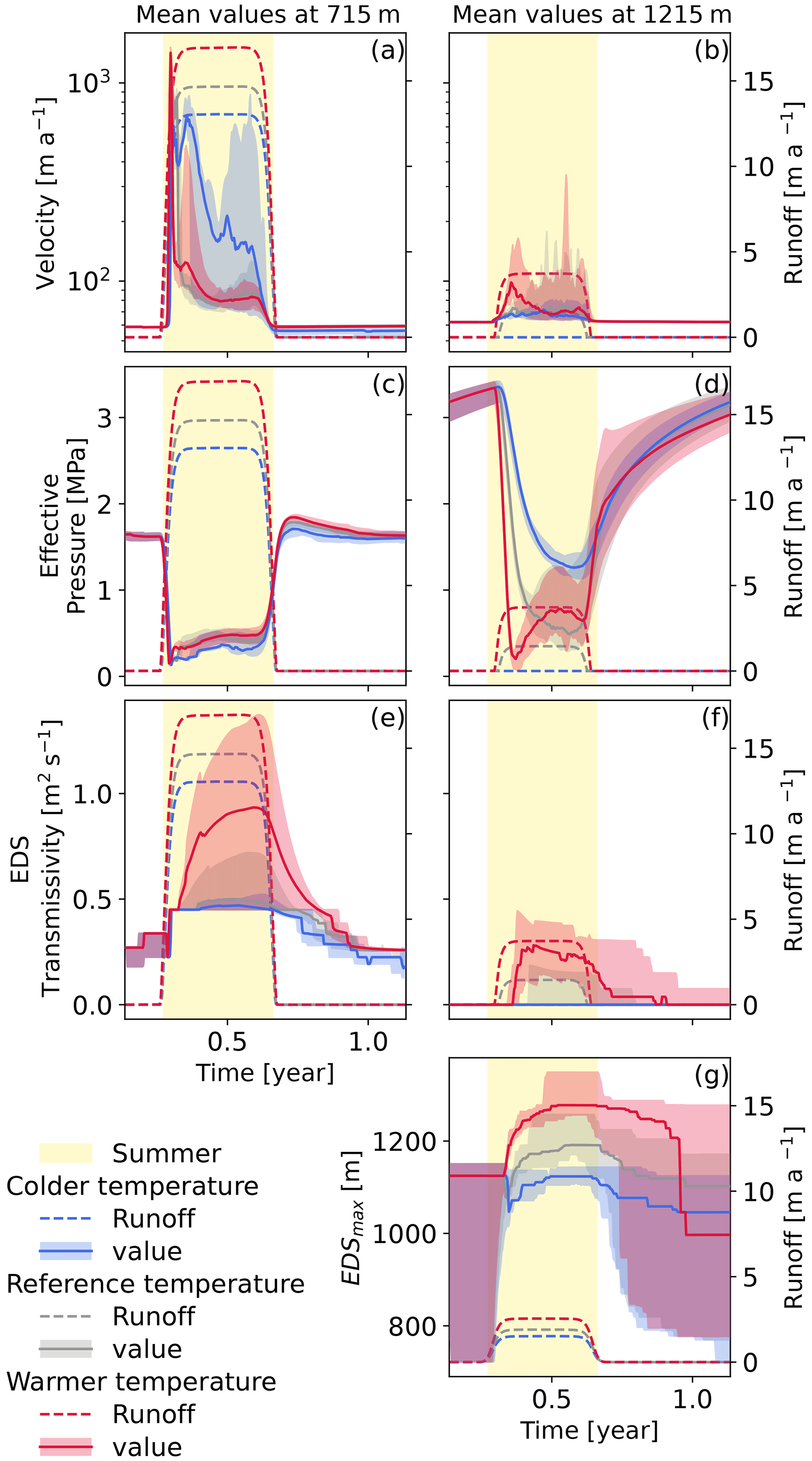
Figure 7 Evolution of the velocity (a–b), effective pressure (c–d), and efficient drainage system transmissivity (e–f) at two different altitudes. Evolution of the maximum height of the active EDS (g). Every panel shows the reference simulation in grey, the higher-intensity melt season in red, and the lower-intensity melt season in blue. The same color scheme is used for the runoffs which are shown as dashed lines and are referenced on the right axis. The yellow shading corresponds to the fixed summer duration as defined in Sect. 2.3.

Comparing the simulations with different intensities yields larger differences between simulations (Fig. 7). We find here a similar pattern to the simulations with varying intensity and duration (Sect. 3.2). At low elevation the initiation of the melt season yields the same pattern with a strong spring speedup which is followed by a secondary acceleration in the case of the low-intensity forcing (Fig. 7a). The higher-intensity melt season also shows a marked overshoot of the winter effective pressure value at the end of the melt season (Fig. 7c). Above SSU_max the difference in the melt intensity means that the experiments with the lower intensity do not experience runoff at this elevation. This leads to the effective pressure in this case being driven by the downstream evolution of the effective pressure which results in a slow decrease in the effective pressure throughout the melt season (Fig. 7d). The velocity response follows the variations in effective pressure with a slow increase towards a rather low maximum summer velocity towards the middle of the melt season (Fig. 7b). Despite showing some recharge at this elevation, the reference simulation shows a similar velocity pattern as the meltwater availability at this altitude does not lead to very low water pressures. The response to the more intense (warmer) melt season is quite different. Here the water input is sufficient to drive a quick drop in effective pressure and the following rebound once the efficient drainage system is activated (Fig. 7f). In term of velocities, that translates to a spring acceleration of small magnitude with gentler slopes than what is observed on the lower part of the glacier.

Table 5 Velocity difference from the reference simulation for different intensities of the melt season with the reference duration. The values in bold fonts are the simulations for which the difference with respect to the reference simulation is significant as per a Wilcoxon test with p=0.01. The summer and winter are defined as fixed periods, with summer starting on day 100 and ending on day 241, while winter covers the rest of the year.

The general impact of the melt season intensity on the glacier's velocity shows counter-intuitive results (Table 5). The mean velocities over the whole domain indicate here that the stronger-intensity forcing does not lead to any significant difference in velocity compared to the reference simulation. However, the melt season with lower intensity shows a substantial increase in the mean annual velocities. This acceleration is mostly due to a two-fold increase in the summer velocities at low elevation, which in our experiments can not be offset by the slowdown at higher elevation or during winter. The increase in the melt area that is driven by the larger intensity of the melt season drives an acceleration of the upper part of the glacier, but this acceleration is not sufficient to impact the overall velocity of the glacier.

Figure 8 summarizes the effect of intensity and length of the melt season on both the subglacial hydrology system and the glacier dynamics. In Fig. 8a we see a clear linear relation between the increase in the runoff volume and the transmissivity of the efficient drainage system, which shows that on the whole glacier, an increase in meltwater volume leads to a more developed subglacial drainage system either in areal extent (increase in EDS_max) or transmissivity of the system. This relationship is not related to the distribution of the melt throughout the year, and we see that an increase in runoff driven by either a longer melt season (growing marker sizes) or an intensifying melt season (darkening markers) leads to a similar increase in transmissivity.

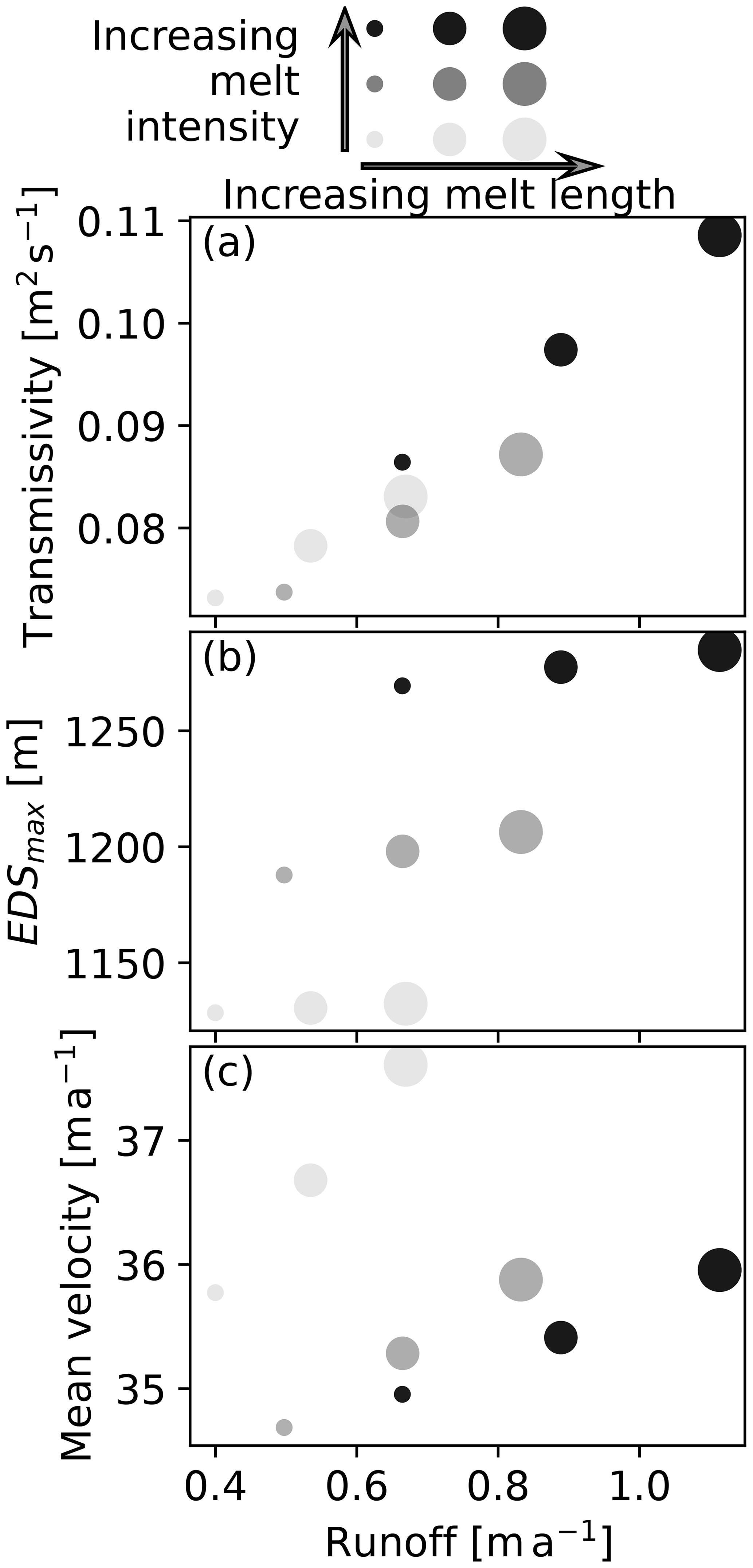
Figure 8 Evolution of the subglacial drainage transmissivity (a), of the maximum elevation at which the efficient drainage system is active (EDS_max) (b), and of the mean glacier velocity (c), function of the mean glacier runoff. The different shades of grey represent different melt intensities, with the low intensity being lighter than the high intensity. The size of the marker represents the length of the melt season, with bigger markers corresponding to longer melt seasons.

The response is more contrasted for the areal development of the efficient drainage system. This characteristic is described by EDS_max (Fig. 8b), the maximum altitude of the glacier surface under which the efficient drainage system is active. As for the transmissivity, Fig. 8b shows that the efficient drainage system develops further upstream if the increase in runoff is due to an increase in the intensity of the melt season. However, EDS_max shows a more gradual increase if the runoff is only increased by a lengthening of the melt season. A result of these two different behaviors is that for a given runoff, the spread of the efficient drainage system will be greater for a short and intense melt season (small black dot in Fig. 8b) than for a long and less intense melt season (big light-grey dot in Fig. 8b). The interplay between these two relations leads to a complex relationship for the mean velocity of the glacier as seen in Fig. 8c. In our experiments, and if the intensity of the melt season is fixed, an increase in runoff and so a longer melt season will lead to an increase in the glaciers' velocity. However, for a fixed season length an increase in the melt intensity first drives a sharp decrease in velocity followed by a slow velocity increase. Focusing again on a constant runoff, the velocities in our model are increasing if the length of the melt season increases. That is the reverse scenario of the one of EDS_max, which was expected. Indeed, a more widespread efficient drainage system allows a larger amount of water to be drained away and in the end allows the velocities during summer to settle at a lower point than on a glacier with a lower effective pressure.

3.4 Initiation length forcing

The definition of our forcing means that a change in amplitude would lead to small variations in the steepness of the initiation of the melt season. In order to evaluate the effect of this change in the recharge increase, here we present a set of experiments in which the length of the initiation has been changed, which leads to initiations with different rates. Figure 9 shows the evolution for simulations in which the initiation rate is altered from the common reference. These simulations have a common runoff, which means that the simulation set with the shorter initiation has the lowest melt intensity.

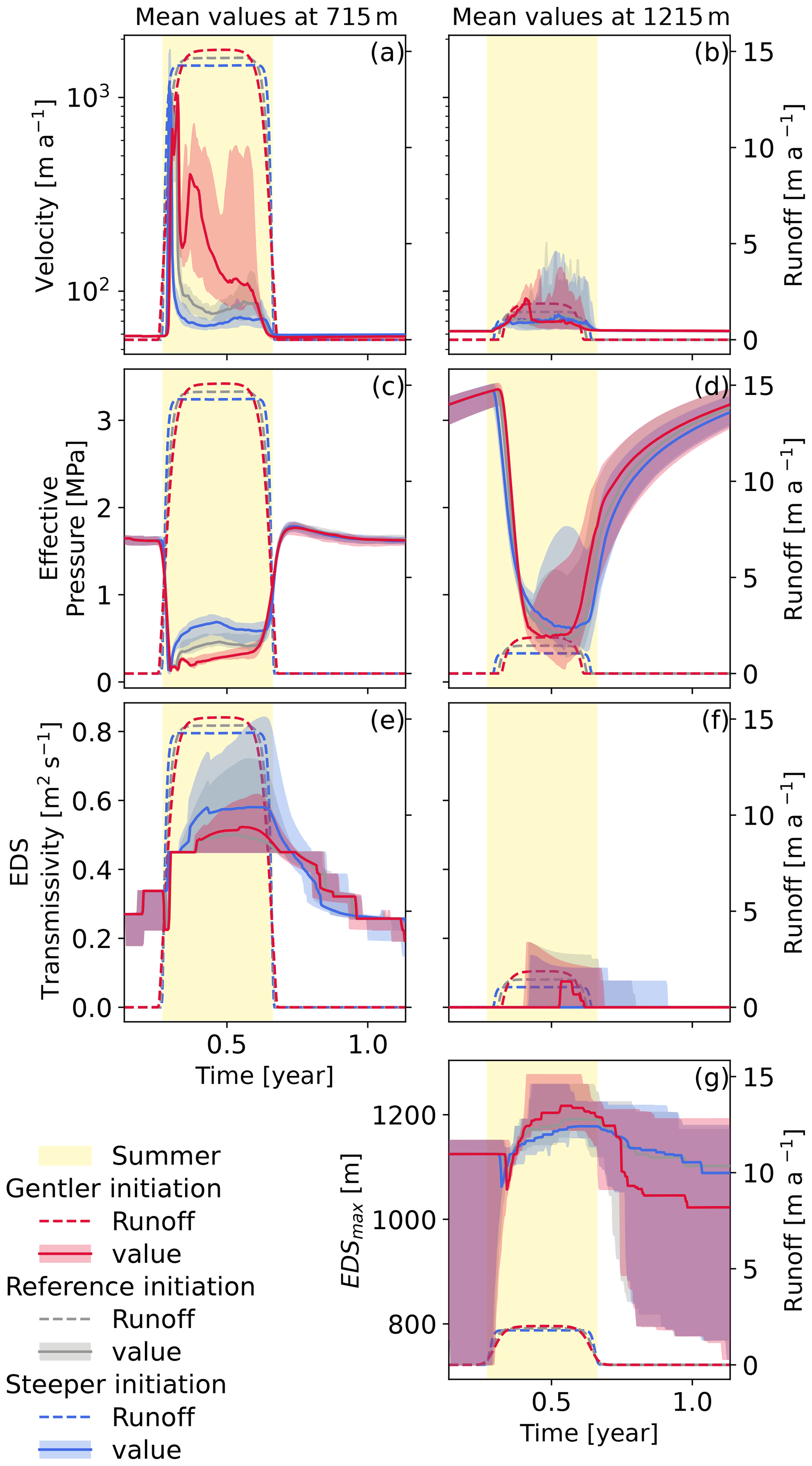
Figure 9 Evolution of the velocity (a–b), effective pressure (c–d), and efficient drainage system transmissivity (e–f) at two different altitudes. Evolution of the maximum height of the active EDS (g). Every panel shows the reference simulation in grey, the longer initiation period in red, and the shorter initiation period in blue. The same color scheme is used for the runoffs which are shown as dashed lines and are referenced on the right axis. The yellow shading corresponds to the fixed summer duration as defined in Sect. 2.3.

At low elevations, the simulations with the steeper initiation show a very sharp and short-lived spring speedup Fig. 9a. That contrasts with the simulation with a more gentle initiation in which the spring speedup reaches lower peak velocities and has a longer duration with a secondary peak later in spring. Figure 9a also shows that with a steeper initiation the velocities after the initial speedup are relatively slow, which contrasts with the more gentle speedup in which a number of the ensemble members show quite high velocities throughout the melt season. These two contrasting responses can be explained by the development speed of the efficient drainage system as seen in Fig. 9e. The simulations with steep initiation periods show the fast development of a very efficient drainage system, whereas the simulations with longer initiation periods show a later development of a less efficient drainage system. This difference explains why the effective pressure in the case of the steep initiation simulation shows a very steep rebound to a rather high summer value for the effective pressure, while the effective pressure for a more gentle melt season initiation stays rather low throughout the summer, which drives the observed fast velocities. The development of an efficient draining system with a low draining capacity in the case of the gentle initiation also leads to a large migration upstream of this system, and its limited efficiency produces low effective pressures on the higher part of the glacier if compared to a fully developed efficient drainage system.

We see in Table 6 that the effect of a change in the initiation length only impacts significantly the lower part of the domain where the efficient drainage system controls the effective pressure response. The domain means show that the gentler initiation has a larger impact on the velocities with an acceleration of roughly 15 %, whereas the steeper initiation only drives a 6 % decrease in ice velocity.

Table 6 Velocity difference from the reference simulation for initiation period length. The values in bold fonts are the simulations for which the difference with respect to the reference simulation is significant as per a Wilcoxon test with p=0.01. The summer and winter are defined as fixed periods, with summer starting on day 100 and ending on day 241, while winter covers the rest of the year.

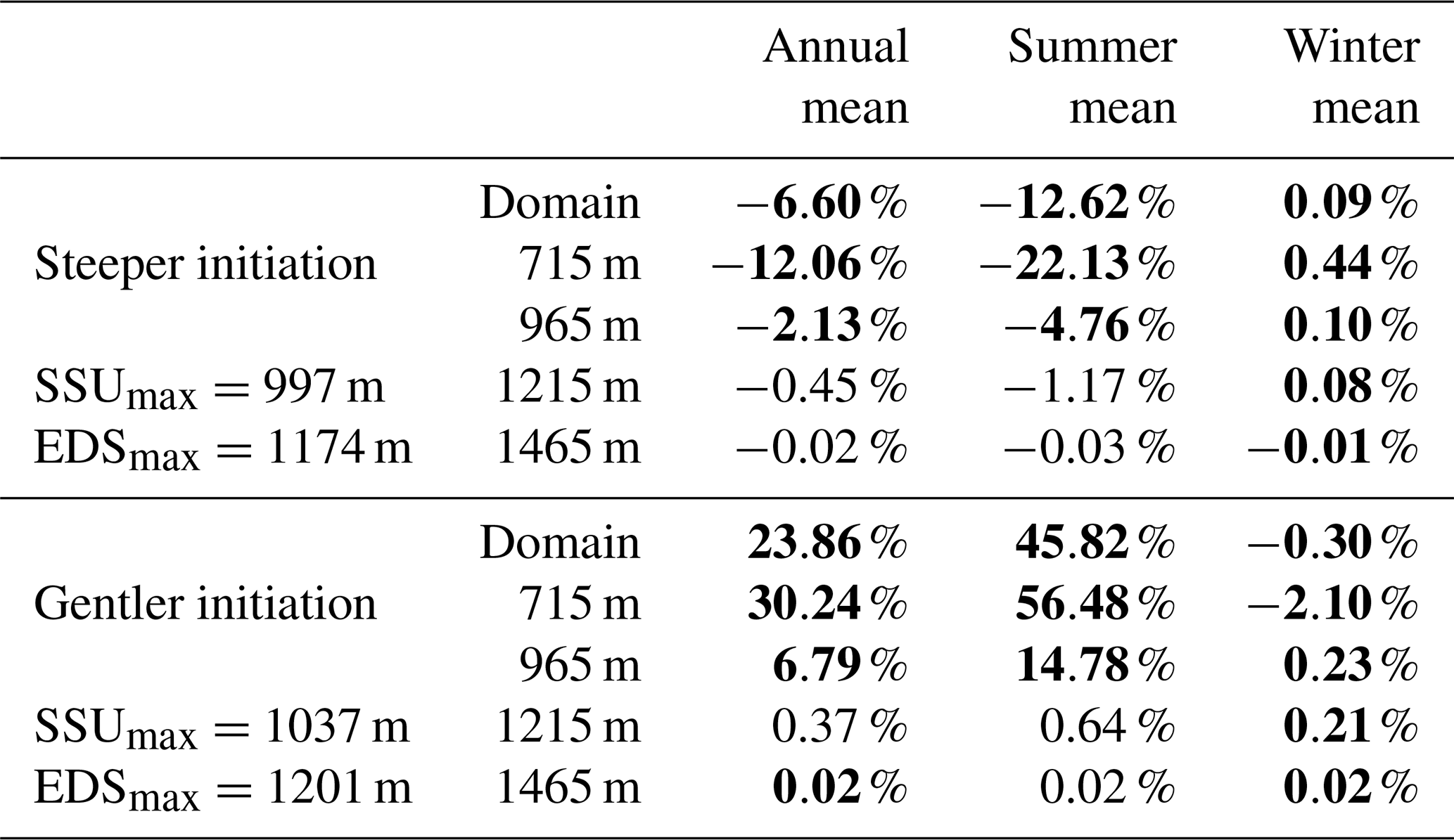
It is interesting here to compare these results with the ones from the preceding experiment (Fig. 7c). In Fig. 9c the simulation with the lowest intensity (sharper initiation) shows a behavior that is closer to the one with the highest intensity (which is also the one with the sharper initiation) in Fig. 7c, where the drop in effective pressure is quickly followed by a fast rebound to rather high summer velocities.

This reinforces the hypothesis that the rate of recharge of the subglacial drainage system might have a similar or even a larger impact than the volume of water that is actually injected into the system (Bartholomaus et al., 2008; Hoffman et al., 2011; Bartholomew et al., 2012; Cowton et al., 2016).

4 Discussion

As with any modeling study, the results presented here might be impacted by the model design and the experiment setup. It is important to note that subglacial hydrological models have not converged in a standard way to treat the subglacial drainage system yet, and the SHMIP exercise (de Fleurian et al., 2018) has shown that there are some discrepancies between the different approaches. However, the agreement of the results presented here with existing theories and observations of subglacial drainage, as well as the physical explanation of the modeled results, give us confidence in their robustness.

The results of our model suggest that the relationship between ice velocity and meltwater runoff is also strongly influenced by the distribution of the melt during the year. Hence if an increase in runoff is driven by a longer melt season, the mean annual velocities of the glaciers will show a strong increase at all elevations. However, an increase in the intensity of the melt season first drives a reduction in the ice velocities before they start to increase again with what seems to be a lower rate. The mean annual velocities can however not explain the complexity of the lubrication feedback. The effect of a change in the length of the melt season has a similar effect on all regions of the glacier, and the velocity increases linearly with the length of the melt season (Table 4). This differs from the response to an increase in the intensity of the melt season. There the response is different at low elevations, where the subglacial drainage is controlled by the efficient components, and at high elevations, where the drainage is controlled by the inefficient components. At higher elevations, our results compare well with those of Gagliardini and Werder (2018) in which we see that an increase in the recharge in the regions controlled by the inefficient drainage system leads to an acceleration of the glacier. However, at lower elevations our results diverge from preceding studies. In the lower parts of the glacier, where the subglacial drainage is controlled by an efficient drainage system, an increase in the intensity of the melt season leads to a decrease in the ice flow velocities. We explain this result through the evolution of the efficient drainage system in those simulations (Fig. 7e–g). In these figures we can see a faster development of the efficient drainage system to higher elevations for the more intense melt season. The development of this system leads to an increase in the effective pressure on the lower part of the glacier, and so it keeps the velocities at levels that are comparable to the ones of our reference simulations. In the case of the low-intensity melt season, however, the water recharge is not sufficient to trigger the development of a well-developed efficient drainage system, which leads to low effective pressures throughout the melt season which in turn induce a large increase in velocities compared to our reference simulation. It must be noted however that these conclusions only hold on seasonally averaged velocities and that a higher-intensity runoff will lead to higher maximum velocities.

We can see the effect of the rate of recharge on the experiments in which the length of the initiation of the melt season was changed (Fig. 9). These results can be compared to the observations made on lake drainage by Tedesco et al. (2013b), in which a fast-draining lake triggered a large and short-lived speedup, while a slower-draining lake only generated a mild speedup after which the velocities stabilized at a higher level than what was recorded before the lake drainage. In this case, the variation in the duration of the initiation of the melt season leads to quite large variations in the overall velocities of the glacier. Here, the sharper initiation leads to slower velocities, but this simulation also has a slightly smaller amplitude to keep the overall runoff identical for all simulations. This is in contradiction to the preceding experiments in which the smaller amplitudes were driving a faster glacier. But the similarities here lie in the sharpness of the runoff curve at the beginning of the melt season. Hence a sharp rise in the temperatures at the beginning of the melt season has the potential to produce a large amount of meltwater which in turn could trigger an early activation of the subglacial drainage system and lead to gentler velocities throughout the summer (after a large spring speedup event). However, the slope of the temperature rise at the beginning of the melt season is highly variable and complex to characterize in the existing dataset, which makes it problematic to provide reliable estimates of the impact of this parameter on the lubrication feedback. The large impact of this small variation also poses the question of the response of the model to more realistic forcings, in which the water presents some short-term temporal variability that is not introduced here.

In our model, the observed mean velocities are mainly driven by the lower regions of the glacier where the velocities are significantly higher. That is clear when comparing the velocity evolution at different altitudes to the domain mean velocity in Fig. 3. This explains why in our model the mean velocities are largely influenced by the activation of the efficient drainage system which in turn is tightly linked to the intensity of the melt season. Another subglacial hydrology model, producing lower effective pressure at higher elevation as seen in the SHMIP intercomparison exercise (de Fleurian et al., 2018), could lead to a preponderant effect of higher elevation velocities which might yield different conclusions on the relationship between runoff distribution and glacier velocity.

The results that we observe could also be biased by the setup of our experiments in which the recharge of the subglacial drainage system has the same spatial distribution and timing as the surface runoff. This is not what is expected in a natural setting where water produced at the surface will transit at the surface of the ice for a given time before traversing the ice through moulins and entering the subglacial drainage system through these localized injection points. Scholzen et al. (2021) showed a limited impact on the subglacial drainage system between simulations performed with a spatially homogeneous or discrete basal recharge. Their results show a difference in the timing of the effective pressure response to the runoff but only slight variations in amplitude or length of the pressure pulse. This is coherent with the results of the SHMIP intercomparison (de Fleurian et al., 2018) in which the moulin distribution did not impact the overall spatial distribution of the effective pressure unless an unrealistically low number of moulins was used. Both those results reassure us that the result presented here should be robust and should not be altered in a major way if one decides to introduce a supraglacial and intraglacial component to the hydrology model.

Due to the way in which we prescribe the model's recharge, the highest injection point in our simulation is varying with the intensity of the melt season from 1209 m of elevation for the low-intensity melt season to 1355 m of elevation for the more intense melt season. However, if the supraglacial and intraglacial drainage are considered, it is most likely that the highest injection point would not change on a yearly basis to adapt to the changes in the melt season but rather follow the migration of moulins at the surface of the glacier. For example, Gagliardini and Werder (2018) modeled moulin migration rates from roughly 1 to 10 m of elevation per year depending on the setting. Having fixed injection points in our experiments might reduce the increase in the spread of the EDS for the more intense melt season. However, this change would only impact a small area of the glacier with rather low velocity and hence is unlikely to lead to large differences in the overall response of the glacier and the conclusions of this study.

The large difference in behavior between the lower and higher part of the glacier make it challenging to extrapolate the results to a longer-term evolution of the ice dynamics without performing simulations spanning a longer time period. The two different behaviors are tightly linked to the region in which the efficient drainage system develops which itself is quite sensitive to the intensity of the melt season as seen in Fig. 8b. An increase in the length of the melt season should not alter in a large way the spread of the efficient drainage. Moreover, the variation in melt season length is affecting the whole glacier in the same way, so the response here is quite clear, and longer melt seasons should lead to overall faster glaciers. However, it is not expected that the current evolution in climate would only alter the length of the melt season in Greenland. If we expect both intensity and length of the melt season to increase in a similar way, the speedup caused by the increase in melt season length is likely to outweigh the slight (and statistically not significant) slowdown driven by the higher melt season intensity. However, a change in intensity has larger implications for the migration of the efficient drainage system upstream, which could have larger implication on longer timescales. In our experiments, an increase in runoff amplitude leads to a slight slowdown of the glacier which is linked to the larger spread of the efficient drainage system. The large runoff at higher altitudes also drives a faster glacier there, and in the long term that could induce a larger region of faster flow which would lead to faster velocities overall. On the other hand, a longer melt season of lower intensity drives a faster glacier in the marginal region but also shows a decrease in the upstream velocities. This should however be taken with caution as a lowering of the glacier surface would lead to an intensification of the melt, which we have shown to be a potential negative feedback on ice velocities. To better understand the impact of these processes on future Greenland ice sheet velocities, studies could focus on finding out the main expected trends in length and intensity of future melt seasons.

These different scenarios, with counter-intuitive results for the seasonal velocities, show that the full subglacial drainage system, and particularly its efficient component, must be included in studies that aim to quantify the effect of meltwater lubrication feedback.

5 Conclusions

We developed a set of experiments that allows the comparison of the effect of different parameters impacting the distribution of runoff throughout the melt season. The use of forcing scenarios based on the ERA5 reanalysis dataset gives us confidence that the variations in intensity and length of the melt season that we tested here are representative of the range of existing melt seasons. Our results show that under a given runoff volume, an increase in the length of the melt season drives an overall faster glacier. With simulations spanning a range of different runoff intensities we show that an increase in melt intensity initially leads to a higher maximum velocity at low elevations but then translates to a lower mean summer velocity over the whole domain and an overall slowdown of the glacier. This behavior is mostly due to the development of a very transmissive efficient drainage system at low elevations which keeps the effective pressures at a high level throughout the melt season and so leads to relatively low summer velocities when averaged over the whole domain. This study can not give a definite answer on the impact of an increase in runoff on the long-term evolution of glacier velocities. Indeed, the impact of the melt season amplitude is radically different at different altitudes, and these regions are delimited by the existence or not of an efficient drainage system. Our experiments show that an increase in the amplitude of the melt season leads to a larger extent of the region where the drainage is controlled by the efficient subglacial drainage system. This change of regime on the highest regions of the glaciers might significantly alter the velocity profile of the glacier, with regions at higher altitudes then experiencing spring speedup events. The experiments performed with varying slopes for the temperature rise at the beginning of the melt season emphasize once more the potential importance of the short-term temporal variation in water influx which should be investigated further. This finding emphasizes the fact that subglacial drainage models with both inefficient and efficient drainage components should be used if one wants to give an accurate assessment of the effect of meltwater on the overall dynamics of the Greenland ice sheet.